the Creative Commons Attribution 3.0 License.
the Creative Commons Attribution 3.0 License.
Climate impact of idealized winter polar mesospheric and stratospheric ozone losses as caused by energetic particle precipitation
Katharina Meraner
Hauke Schmidt
Energetic particles enter the polar atmosphere and enhance the production of nitrogen oxides and hydrogen oxides in the winter stratosphere and mesosphere. Both components are powerful ozone destroyers. Recently, it has been inferred from observations that the direct effect of energetic particle precipitation (EPP) causes significant long-term mesospheric ozone variability. Satellites observe a decrease in mesospheric ozone up to 34 % between EPP maximum and EPP minimum. Stratospheric ozone decreases due to the indirect effect of EPP by about 10–15 % observed by satellite instruments. Here, we analyze the climate impact of winter boreal idealized polar mesospheric and polar stratospheric ozone losses as caused by EPP in the coupled Max Planck Institute Earth System Model (MPI-ESM). Using radiative transfer modeling, we find that the radiative forcing of mesospheric ozone loss during polar night is small. Hence, climate effects of mesospheric ozone loss due to energetic particles seem unlikely. Stratospheric ozone loss due to energetic particles warms the winter polar stratosphere and subsequently weakens the polar vortex. However, those changes are small, and few statistically significant changes in surface climate are found.
- Article
(2634 KB) - Full-text XML
- BibTeX
- EndNote


Energetic particles enter the Earth's atmosphere near the magnetic poles altering the chemistry of the middle and upper atmosphere. Energetic particle precipitation (EPP) is the major source of nitrogen oxides (NOx) and hydrogen oxides (HOx) in the polar middle and upper atmosphere (Crutzen et al., 1975; Solomon et al., 1981). Both chemical components catalytically deplete ozone; NOx mainly below 45 km and HOx mainly above.
HOx is short-lived in the middle atmosphere and depletes ozone mainly in the mesosphere. In contrast, NOx persists for up to several months in the polar winter middle atmosphere. Inside the polar vortex, NOx can be transported downward from the lower thermosphere to the stratosphere, where it depletes ozone (e.g., Funke et al., 2017; Sinnhuber et al., 2014; Hendrickx et al., 2015). Observational evidence of polar winter stratospheric ozone loss due to EPP is still limited. Only recently have long-term satellite observations with good temporal and spatial coverage become available. In austral polar winter EPP causes an ozone loss of about 10–15 % descending from 1 hPa in early winter to 10 hPa in late winter (Fytterer et al., 2015; Damiani et al., 2016). Extensive information on the current knowledge of energetic particle precipitation can be found in Sinnhuber et al. (2012) and Mironova et al. (2015).
Ozone loss influences stratospheric temperature and the polar vortex. The Northern Annular Mode (NAM) index is often used to describe the strength of the polar vortex, with positive NAM values indicating a strong polar vortex and negative NAM values indicating a weak polar vortex. Observations indicate that anomalous weather regimes associated with the NAM index can propagate from the stratosphere down to the surface (Baldwin and Dunkerton, 2001). Hence, energetic particle precipitation may provide a link from space weather to surface climate. Here, we study the impact of ozone loss due to EPP on the circulation and subsequently on climate. Discussed are both a polar mesospheric and a polar stratospheric ozone loss.
Since the discovery of the ozone hole in the mid-1980s, the climate impact of stratospheric ozone loss has been intensively studied (e.g., Shine, 1986; Randel and Wu, 1999; Lubis et al., 2016). Most studies concentrated on the climate impact of the ozone hole during austral spring and have reported cooling in the spring Southern Hemispheric stratosphere due to reduced absorption of solar radiation and strengthening of the polar vortex. In contrast, our study concentrates on ozone loss during the boreal polar night. During polar night, reduced ozone slightly decreases the infrared cooling of the polar stratosphere resulting in net (small) stratospheric warming (Graf et al., 1998; Langematz et al., 2003). However, both studies prescribed ozone loss in the lower stratosphere.
Several studies have suggested a significant influence of EPP on climate. Seppälä et al. (2013) and Lu et al. (2008) used reanalysis data to investigate the dependence of stratospheric temperature and zonal wind on the Ap index. They found stratospheric warming of up to 5–10 K for strong energetic particle precipitation descending from the stratopause to the mid-stratosphere. However, for the zonal wind response the two studies differ from each other. Seppälä et al. (2013) found strengthening of the polar vortex, whereas Lu et al. (2008) showed weakening of the polar vortex. Moreover, Seppälä et al. (2009) analyzed surface air temperature changes in reanalysis data for years with various strengths of EPP. They found warming over Eurasia and cooling over Greenland for winters with enhanced EPP, but could not rule out that the estimated changes are induced by NAM variability independent of EPP.
Other studies relied on atmospheric chemistry models, which showed similar surface temperature change patterns as found in the reanalysis data (e.g., Rozanov et al., 2005; Baumgaertner et al., 2011; Arsenovic et al., 2016). They reported small cooling in the polar winter stratosphere due to EPP. However, the radiative effect of a polar night ozone loss should lead to warming, which can also be found in reanalysis data (Lu et al., 2008; Seppälä et al., 2013). The simulated stratospheric cooling is attributed to dynamical, adiabatic cooling caused by a decrease in the mean meridional circulation (Schoeberl and Strobel, 1978; Christiansen et al., 1997). Langematz et al. (2003) suggested that the weaker mean meridional circulation is caused by a decrease in midlatitude tropospheric wave forcing. The aforementioned model studies analyzing the climate impact of EPP relied on relatively few simulation years and applied complex forcings. Instead of prescribing ozone, these studies simulated EPP effects by changing the production of NOx and HOx and modeling the effects on ozone interactively. This could potentially be more realistic than simulations with prescribed ozone anomalies, but it introduces uncertainties related to the representation of chemistry and transport in the model, and renders the understanding of the effects more complicated as the ozone forcing varies in space and time. To avoid these difficulties and to obtain a clear signal-to-noise ratio, we use an idealized ozone forcing and a long simulation period.
Commonly, the effects of EPP are classified into direct and indirect effects (Randall et al., 2006, 2007). Direct effects are those of the local production of NOx and HOx, whereas indirect effects are the effects of the NOx transport from the thermosphere to the stratosphere. Whereas most of the abovementioned studies discuss a mainly stratospheric ozone loss due to the indirect EPP effect, Andersson et al. (2014) suggested a potential climate influence of mesospheric ozone loss due to the direct EPP effect. By using satellite observations they showed that HOx causes long-term variability in mesospheric ozone of up to 34 % between EPP maximum and EPP minimum. Arsenovic et al. (2016) were the first to include the direct effect of HOx local production due to EPP in a chemistry–climate model. They found a similar mesospheric ozone loss as Andersson et al. (2014) and ultimately, reported cooling over Greenland and warming over Eurasia. However, Arsenovic et al. (2016) also considered the indirect effect of the NOx descent. Hence, the sole impact of mesospheric ozone loss due to the direct EPP effect as suggested by Andersson et al. (2014) remains unclear.
This paper studies the circulation and climate impact of idealized mesospheric and stratospheric ozone losses that could be attributed to energetic particle precipitation. We use simulations with the Max Planck Institute Earth System Model (MPI-ESM), applying an idealized ozone forcing in either the mesosphere or the stratosphere. The idealized mesospheric ozone loss that we prescribe may be considered to be mostly a direct EPP effect, whereas the prescribed stratospheric ozone loss should be considered indirect. Additionally, we use a radiative transfer model to quantify the radiative forcing of ozone at different altitudes and months. Ultimately, we discuss whether ozone loss in the middle atmosphere due to EPP has the potential to significantly alter the surface climate. Section 2 describes the MPI-ESM as well as the radiative transfer model. Section 3 links mesospheric and stratospheric ozone losses to changes in the atmospheric temperatures and winds. Finally, Sect. 4 summarizes and discusses the main outcomes and limitations of this study.
2.1 MPI-ESM: the Max Planck Institute Earth System Model
The MPI-ESM (Giorgetta et al., 2013) consists of the coupled atmospheric and ocean general circulation models, ECHAM6 (Stevens et al., 2013) and MPIOM (Jungclaus et al., 2013), the land and vegetation model JSBACH (Reick et al., 2013), and the model for marine bio-geochemistry HAMOCC (Ilyina et al., 2013). We use the “mixed-resolution” configuration of the model (MPI-ESM-MR). The ocean model uses a tripolar quasi-isotropic grid with a nominal resolution of 0.4∘ and 40 vertical layers. ECHAM6 is run with a triangular truncation at wave number 63 (T63), which corresponds to 1.9∘ in latitude and longitude. The vertical grid contains 95 hybrid σ-pressure levels resolving the atmosphere from the surface up to 0.01 hPa. The vertical resolution is nearly constant (700 m) from the upper troposphere to the middle stratosphere, and is less than 1000 m at the stratopause. The time steps in the atmosphere and ocean are 450 and 3600 s, respectively.
The model has been used for many simulations within the CMIP5 (Coupled Model Intercomparison Project Phase 5) framework (Taylor et al., 2012). An overview of the dynamics of the middle atmosphere in these simulations is given by Schmidt et al. (2013). In this study, the preindustrial CMIP5 simulation (piControl) is used as reference. The forcing is constant in time and uses pre-industrial conditions (AD 1850) for the greenhouse gases. Solar irradiance and ozone concentrations are averaged over a solar cycle (1844–1856 for the solar irradiance and 1850–1860 for ozone concentrations). No volcanic forcing is applied. A period of 150 years of this simulation is used.
In order to analyze the impact of ozone changes on the model climate, two additional experiments with reduced ozone concentration are carried out. In one experiment, the mesospheric ozone is reduced by 40 % between 0.01 and 0.1 hPa polewards of 60∘ N (this is called “meso-O3”). In the other experiment, stratospheric ozone is reduced by 20 % between 1 and 10 hPa polewards of 60∘ N (this is called “strato-O3”). We perform on–off experiments, whereas in reality EPP causes a constant (but variable) ozone loss. However, the magnitude of the prescribed ozone losses is based on satellite observations for winter conditions between years with high geomagnetic activity and years with low geomagnetic activity. In general, the impact of energetic particles is sporadic in the mesosphere; Andersson et al. (2014), however, showed that the direct HOx effect induces long-term variability in mesospheric ozone of up to 34 % from November to February in satellite data. Fytterer et al. (2015) and Damiani et al. (2016) revealed an upper stratospheric ozone loss between 10 and 15 % due to energetic particles for the Antarctic high latitudes in long-term measurements. Note that the applied ozone losses are slightly larger than the EPP influence diagnosed from observations. We use the stronger forcing to obtain a clear signal-to-noise ratio. However, this implies a potentially overestimated climate response.
To facilitate experiment design, we fixed ozone losses to be constant over time. Although we concentrate our analysis on boreal winter high latitudes, this still allows us to gain insights into boreal spring (i.e., the transition time from polar night to polar day). Observed ozone losses in summer are in general smaller than during winter, but this idealized setting allows for easy comparison of potential effects during the different seasons. In order to test whether the winter response is influenced through preconditioning, in this experiment design we repeated the experiments with ozone losses prescribed only from December to March. However, as the results are qualitatively very similar and differ only in the magnitude of the responses, we discuss only the results of the experiments with ozone losses prescribed all year. Both experiments, with mesospheric and stratospheric ozone loss, are forced by the same conditions as the piControl experiment. Moreover, the simulations are restarted from the same year in the piControl experiment. This ensures that the ocean state is similar in all experiments. For both simulations 150 years are simulated.
The simplistic nature of our experiments is intentional and, we think, useful. We chose this idealized experimental design in order to separate the climate impact of stratospheric and mesospheric ozone loss due to EPP and to identify the relevant mechanism which determines how EPP affects the climate. Prescribing complex ozone reductions that vary in space, by season and year, or simulating the ozone reduction interactively might enable more realism, but they do not facilitate the identification of potential mechanisms. However, due to the simplification we cannot consider all features associated with EPP. In particular, three main effects are not taken into account: (a) energetic particles entering the atmosphere only over the auroral oval regions (Hendrickx et al., 2015; Fytterer et al., 2015); (b) the negative ozone signal due to EPP propagating from the stratopause in mid-winter to the lower stratosphere in spring within the polar vortex (Funke et al., 2017; Damiani et al., 2016); and (c) that the polar vortex can shift off the pole to regions with more solar radiation. We, instead, apply constant ozone reduction between the stratopause and mid-stratosphere (1–10 hPa) over the entire polar cap. The climate response in our simulations is likely overestimated as we reduce ozone over a larger latitudinal and altitude region than observations suggest.
In Sects. 3.2 and 3.3 the differences between the experiments and the control simulation (i.e., piControl) are analyzed. Statistical significance is calculated using the 95 % confidence intervals assuming normally distributed regression errors and using the 0.975 and 0.025 percentile of Student's t distribution with the appropriate degrees of freedom. Properties of two simulations are considered statistically significantly different if the mean value of the control simulation is outside 95 % confidence interval of the experiment.
2.2 The radiative transfer model PSrad
The radiative transfer scheme of MPI-ESM is based on the rapid radiation transfer suite of models optimized for general circulation models (RRTMG; Mlawer et al., 1997; Iacono et al., 2008). The RRTMG is widely used and its ability to calculate radiative forcing has been evaluated by Iacono et al. (2008). In its stand-alone version here, it is used to study the impact of ozone on heating rates. It is divided into 16 bands in the longwave (1000–3 µm) and 14 bands in the shortwave (12 195–200 nm; Clough et al., 2005). The spectral bands are chosen to include the major absorption bands of active gases. The major ozone absorption bands – Hartley band (200–310 nm), Huggins bands (310–350 nm), and Chappuis bands (410–750 nm) – are considered. However, absorption of oxygen at shorter wavelengths than 200 nm is missing, which could lead to an underestimation of the total heating rate in the mesosphere. The radiative transfer scheme is further described in Pincus and Stevens (2013) and Stevens et al. (2013), and further on we will refer to it as the radiative transfer model “PSrad”.
The shortwave and longwave components are calculated separately. Furthermore, optical properties for gases, clouds, and aerosols are computed separately for longwave and shortwave components and, finally, combined to compute the total heating rates. PSrad expects profiles of gases (H2O, N2O, CH4, CO, O3), profile of cloud parameters as well as additional parameters (e.g., albedo and zenith angle) as input. Additionally, CO2 and O2 are set to fixed values invariant with height. For all other gases, we use multi-year monthly means representative of the late 20th century provided by the atmospheric and chemistry model HAMMONIA (Hamburg Model for Neutral and Ionized Atmosphere; Schmidt et al., 2006). For the albedo and cloud properties (e.g., cloud fraction, cloud water/ice content), multi-year monthly means from the piControl experiment are used. All quantities are extracted for 75∘ N. The zenith angle is calculated for 12:00 UTC at 75∘ N, 0∘ E for the 15th of each month. The latitude of 75∘ N is chosen to be exemplary for polar latitudes. The results are insensitive to the actual latitude, the main difference at other polar latitudes is the length of the polar night. Note that the length of the polar night for an air pocket also depends on the altitude and on atmospheric dynamics (e.g., movement of the polar vortex). Both effects are omitted in this study. In our simulations ozone is reduced independent of actual dynamics, over the entire polar cap (60–90∘).
To quantify the impact of ozone on the heating rates, we perform multiple runs in which for each run the ozone concentration of a single layer is set to 0. Then we take the differences between a control run and each single run. The differences of each run are, finally, added up for the estimation of the total heating rate. This method allows us to consider that layers of reduced ozone will lead to increased absorption of shortwave radiation in the layers directly below.
3.1 Ozone effects on the heating rates
Ozone loss directly alters the atmospheric energy transfer. Before analyzing circulation and climate impacts due to ozone losses, we study the heating rate response using the radiative transfer model PSrad. The heating rates are calculated for the polar latitude of 75∘ N (see Fig. 1). As the effect of EPP is most important at the winter polar cap, we will concentrate our analysis on boreal winter high latitudes.
In the shortwave part of the spectrum, ozone strongly absorbs solar radiation and heats the whole atmosphere. The strongest heating (about 12 K day−1) occurs in the uppermost stratosphere around 1 hPa. Ozone loss would, hence, result in relative cooling due to reduced heating. The ozone heating and, hence, the cooling caused by ozone reduction become smaller for larger zenith angles and vanish in polar night.
In the longwave part of the spectrum, the radiative effect of ozone is highly temperature dependent. Ozone cools the atmosphere via infrared emission in the stratosphere and in warm regions of the mesosphere below 0.1 hPa (see Fig. 1b). The strongest cooling (about −2 K day−1) occurs at the stratopause. In the troposphere and in the cold regions of the mesosphere above 0.1 hPa, the absorption of outgoing radiation exceeds the infrared emission resulting in a heating of the atmosphere due to ozone.
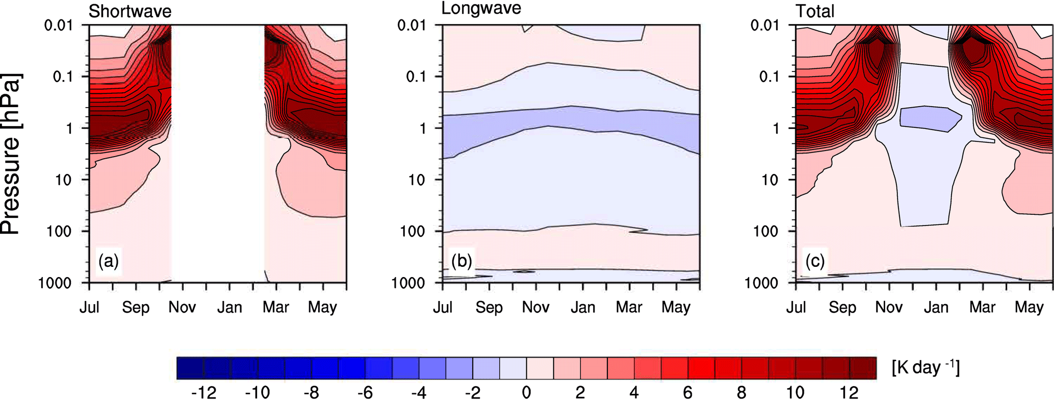
Figure 1Monthly mean heating rates of ozone (K day−1) for 75∘ N calculated by the radiative transfer model PSrad for (a) shortwave, (b) longwave, and (c) total (shortwave + longwave) radiation.
In total, the shortwave heating dominates all sunlit months. During polar night, ozone cools the atmosphere between 0.1 and 100 hPa and, hence, ozone loss in the stratosphere and lower mesosphere results in warming. Near the terminator (e.g., at 75∘ N in November and February), the net influence of ozone is more complex: at some altitudes ozone heats the atmosphere and at some ozone cools it. The net radiative forcing of ozone loss depends on when and where ozone is reduced. For example, in November, stratospheric (1 hPa) ozone loss leads to a heating, but mesospheric (0.1 hPa) ozone loss leads to cooling.
These results are in line with previous work. It is widely accepted that ozone loss in spring and summer leads to stratospheric cooling (e.g., Shine, 1986; Randel and Wu, 1999). Some studies analyzed the radiative forcing of winter stratospheric ozone loss. Graf et al. (1998) showed that the observed stratospheric ozone loss in the late 20th century led to winter warming and summer cooling in a global climate model. Using a radiative transfer model with fixed dynamical heating, Langematz et al. (2003) confirmed that stratospheric ozone loss over the winter pole results in small stratospheric radiative warming and dominating stratospheric dynamical cooling. Shine (1986) showed that the shortwave cooling of the stratosphere due to ozone loss dominates, in all sunlit months, infrared heating due to ozone loss. Recently, Sinnhuber et al. (2017) simulated warming in mid-winter and cooling in late winter and spring in the upper stratosphere for ozone losses explicitly induced by EPP.
The results above are confirmed by the actual heating rate anomalies induced by the applied ozone losses in the experiments meso-O3 and strato-O3 (not shown). The heating rates are calculated at the first time step of the model at which the radiation is updated (1 January) excluding any feedbacks occurring only at later time steps. Note that the exact values may change for other months, especially depending on the sunlit area. Compared to the total heating rates of piControl, the changes in heating rates caused by a 40 % reduction of mesospheric ozone in polar night are very small (on average about −0.01 K day−1 and −0.4 %), and by a 20 % reduction of stratospheric ozone on average are about 0.12 K day−1 and 2.6 %. This agrees with the estimate of Sinnhuber et al. (2017), who simulated a change of 0.1 K day−1 in the winter stratospheric heating rate due particle-induced ozone loss. The change in heating rates due to the stratospheric ozone change is in the range of solar UV forcing (0.1 K day−1) (Gray et al., 2010).
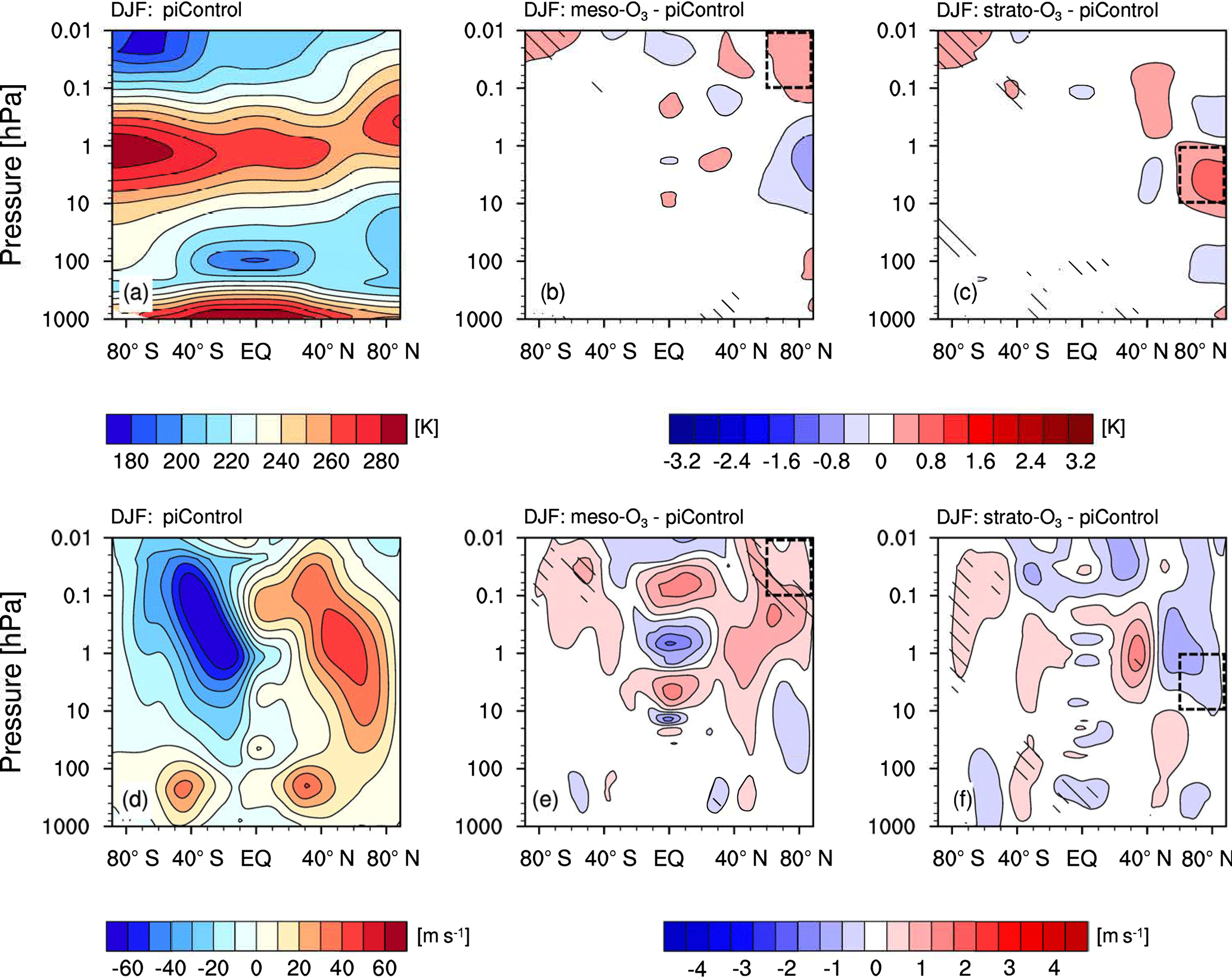
Figure 2Zonal mean temperature (K; top row) and zonal mean zonal wind (m s−1; bottom row) averaged over December–February (DJF) for (a, d) piControl, (b, e) the difference between meso-O3 and piControl, and (c, f) the difference between strato-O3 and piControl. Shaded areas are statistically significant at the 95 % confidence interval. The black, dashed boxes highlight the regions where ozone is reduced.
3.2 Climate effects of mesospheric ozone loss
As changes in heating rates due to reduced ozone during polar night are small, one might reason that climate impact of winter polar ozone loss is small. But large effects may occur in regions slightly outside the polar night. Furthermore, several studies suggested that changes in the heating rates due to winter polar ozone loss leads to dynamical cooling (e.g., Langematz et al., 2003; Baumgaertner et al., 2011; Arsenovic et al., 2016), whereas the initial radiative forcing suggests warming. Hence, we further analyze the climate impact of winter polar ozone loss. As large variations in the polar vortex can propagate downward and affect the surface climate, we first concentrate on the circulation changes of the middle atmosphere due to ozone loss, which are a prerequisite for a potential climate impact of EPP. In the following, we analyze the climate effect of idealized polar mesospheric ozone loss, while in Sect. 3.3 we analyze the climate effect of idealized polar stratospheric ozone loss.
Figure 2a and 2d show the zonal mean temperature and zonal wind simulated for boreal winter (December–February). Main observed characteristics of the zonal mean temperature, e.g., the stratopause tilt from the summer towards the winter pole, are well reproduced. The changes in the zonal mean zonal wind are consistent with the temperature changes via the thermal wind balance. In most regions, the difference between meso-O3 and piControl is very small (see Fig. 2b and 2e).
Near the winter pole, a dipole structure emerges with cooling in the upper stratosphere and warming in the mesosphere. According to our radiative transfer calculations mesospheric winter polar ozone loss should lead to cooling. However, the temperature differences are small (below 1 K) and not significant at the 95 % level. As the applied forcing is very small, small and barely significant values are expected. At the winter pole, the polar vortex slightly weakens, whereas the mesospheric winds strengthen; these differences are not significant. The signal is only slightly stronger but still insignificant if winters with major sudden stratospheric warmings (SSWs) are excluded (not shown). As stated above, large variations in the winter polar vortex can propagate to the surface influencing the surface climate. However, the changes reported here are small. The anomalies reaching the troposphere are statistical artifacts. Indeed, the surface temperature reveals no statistically significant change (not shown).
The temperature and wind signals are not statistically significant after 150 simulated years; it nevertheless makes sense to analyze if the signals could have a physical explanation and not be purely accidental. Note that with fewer simulation years apparently very different results can be obtained. Upon analyzing different simulation periods, we obtain mesospheric warming and cooling of apparent significance. Particularly, we calculated a statistically significant weakening of the polar vortex when using only the first 80 simulation years. We cannot identify a model drift in the experiments, which could explain the disagreement between the 150-year and 80-year runs. However, the model simulates variability on timescales up to multi-decadal, which is common in many climate models (Sutton et al., 2015), and might cause the apparently different responses to ozone reduction in different sub-periods of the 150-year simulation. The high degree of internal variability of the winter polar stratosphere can obviously create incorrect apparent signals. The most dramatic demonstration of this variability are major sudden stratospheric warmings (SSWs), which occur on average about six times per decade in the Northern Hemisphere (see Charlton and Polvani, 2007, for more information on SSW). A short simulation period may lead to an over-representation or under-representation of SSWs. Over our whole simulation period (150 years) the number of major SSWs is balanced in all three experiments. In total, there are 102 events in piControl, 99 events in meso-O3, and 109 events in strato-O3 (using a reversal of the zonal wind at 60∘ N and 10 hPa as the criterion for major SSW occurrence).
3.3 Climate effects of stratospheric ozone loss
In this section, we analyze the climate effect of idealized polar stratospheric ozone loss. Figure 2a and 2d show the zonal mean temperature and zonal wind simulated for boreal winter (December–February) for piControl, and Fig. 2c and 2f show the difference between strato-O3 and piControl. The winter stratosphere warms due to ozone loss as expected from the calculations with the radiative transfer model. As a consequence of the warming, the stratospheric winds weaken. The small mesospheric cooling likely results from enhanced eastward momentum deposition from gravity waves as shown by Lossow et al. (2012). Our results are in line with earlier studies. Seppälä et al. (2013) and Lu et al. (2008) identified warming in the polar winter upper stratosphere due to EPP in reanalysis data, but their magnitude is much stronger (5 K) than in our simulations. Regarding the zonal wind response, the two studies differ from each other. Seppälä et al. (2013) analyzed strengthening of the polar vortex with enhanced equatorward planetary waves, whereas Lu et al. (2008) analyzed weakening of the polar vortex. The statistically significant warming of the summer mesopause is an indication of inter-hemispheric coupling as discussed by Karlsson and Becker (2016) and also persists for winters without a sudden stratospheric warming event.
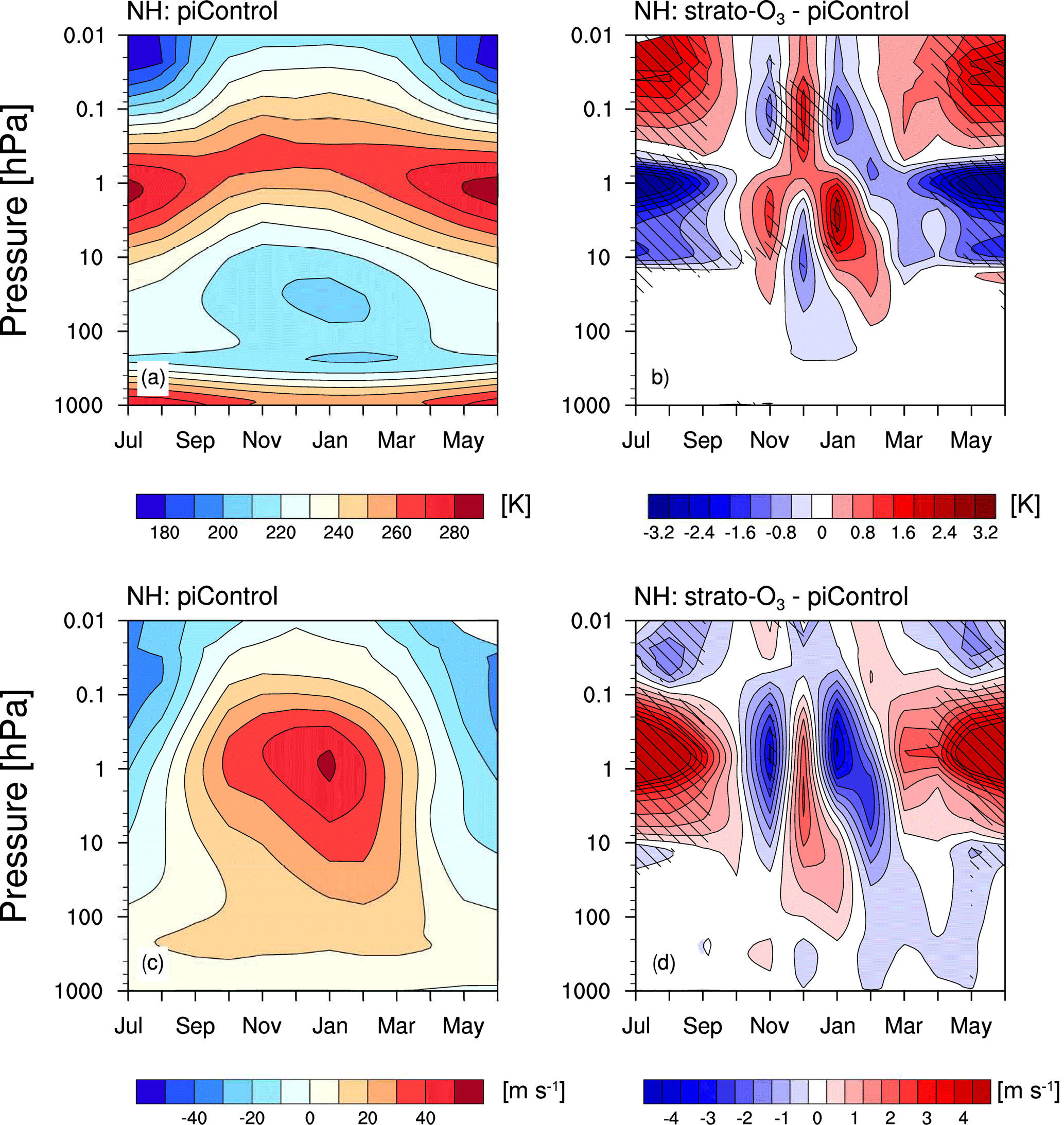
Figure 3Monthly mean temperature (top row) averaged between 60 and 90∘ N (K) and zonal wind (m s−1; bottom row) for 60∘ N for (a, c) piControl and (b, d) the difference between strato-O3 and piControl. Shaded areas are statistically significant at the 95 % confidence interval.

Figure 4Surface temperature (K) averaged over December–February (DJF) for the Northern Hemisphere for (a) piControl and (b) the difference between strato-O3 and piControl. Shaded areas are statistically significant at the 95 % confidence interval.
Figure 2 shows only changes for the mean over December to February, while the radiative transfer model suggests that the month-to-month variability of the forcing is large. To study whether the impact of stratospheric ozone loss differs over the course of the winter, we analyze the monthly means of temperature and zonal wind (see Fig. 3). Ozone loss during most of the polar night (except December) leads to warming, whereas at all other times and locations it leads to cooling. This agrees with the calculations of the radiative transfer model and with our assumption that the winter cooling is not affected by strong summer warming. However, the cooling in December is unexpected from the radiative transfer modeling. Kodera and Kuroda (2002) argued that the polar winter atmosphere transits from a radiatively controlled state in early winter to a dynamically controlled state in late winter. Given the opposite sign of the diabatic forcing, the simulated cooling must have been already dynamically created in December. This is in agreement with early model studies which showed that uniform ozone losses lead to dynamical cooling at the boreal winter polar latitudes (e.g., Schoeberl and Strobel, 1978; Kiehl and Boville, 1988). Langematz et al. (2003) suggested that the dynamical cooling is due to weakening of the mean meridional circulation related to reduced wave forcing caused by a reduction of midlatitude wave flux into the stratosphere. Similarly, in our simulations we find a (albeit not significant) reduction of the zonal mean eddy heat flux at 100 hPa in the midlatitudes from December to March (not shown). This may be caused by enhanced wave reflection as suggested by Lu et al. (2017) for the dynamical response to 11-year solar irradiance forcing. The dynamically induced cooling in December also occurs in simulations in which the ozone is only reduced from December to March (not shown). Also, Baumgaertner et al. (2011) reported dynamical cooling in the winter polar stratosphere due to EPP. However, in their model the cooling dominates the winter (DJF) signal, whereas we obtain small warming for the DJF average (see Fig. 2). The magnitude of the signal decreases in our simulations, especially in late winter, if we exclude all seasons with a SSW (not shown).
The zonal wind changes consistently with the temperature changes via the thermal wind balance. Simultaneously with warming (cooling), the polar wind weakens (strengthens). Anomalies in the polar vortex occasionally reach the troposphere (e.g., the strengthening in November or the weakening in December or February). Although most of those changes are not significant, some disturbances in the polar vortex may still force the surface temperature (see Fig. 4). In our simulations for boreal winter, stratospheric ozone loss cools large parts of the northern high latitudes from northern Europe to Eurasia and over North America. Excluding all winters with a SSW strengthens the cooling over North America (not shown). Over Greenland and the pole, the surface warms. This is consistent with the weakening of the zonal wind in December (see Fig. 3d). However, most changes are small and not significant. Seppälä et al. (2009) and Baumgaertner et al. (2011) analyzed statistically significant changes in surface temperature and found warming over Eurasia of about 1.5 K and cooling over North America of about −1 K. Compared to both studies the amplitude of our signal is much smaller. The weaker signal also persists if we exclude all winters with a SSW (not shown). However, Baumgaertner et al. (2011) based their study on only 9 simulated years and we have shown that the large variability in the polar winter stratosphere can cause incorrect apparent signals if the ensemble is not large enough. Note that another difference between our and their study is that our model is coupled to an interactive ocean. Seppälä et al. (2009) could not rule out that their results are by chance induced by the NAM.
In this study, we analyzed the climate impact of idealized mesospheric and stratospheric ozone losses. Although this study is motivated by the enhancement of NOx due to energetic particle precipitation (EPP), the results presented here could also be applied to other processes causing ozone destruction. We lie the focus on boreal winter. The radiative forcing of polar ozone is calculated by the radiative transfer model PSrad. In sensitivity studies with the Max Planck Institute Earth System Model (MPI-ESM), we applied idealized ozone losses of either 40 % in the winter polar mesosphere or 20 % in the winter polar stratosphere. This simplified design facilitates the identification of the processes relevant for possible climate responses.
Recently, Andersson et al. (2014) showed that the direct EPP-HOx effect induces large long-term variability in winter mesospheric ozone. They suggested that these large changes may have an impact on climate. Following their idea, we analyzed the atmospheric response to mesospheric ozone loss. We found that the winter atmospheric changes due to mesospheric ozone loss in our model are negligible. Calculations with a radiative transfer model showed that the radiative forcing of mesospheric ozone is very small during polar night, which makes the small dynamic response plausible.
Several studies have analyzed the climate effect of stratospheric ozone loss due to EPP. Seppälä et al. (2009) calculated a correlation of the winter surface temperature and energetic particle precipitation in reanalysis data. However, they could not rule out accidental correlation. Since then several model studies have tried to establish a physical link between EPP and climate (Baumgaertner et al., 2011; Rozanov et al., 2012; Arsenovic et al., 2016). In all these model studies, dynamical cooling of the winter polar stratosphere due to energetic particle precipitation was simulated. In our model, stratospheric ozone loss during polar night (except December) results in warming, whereas at all other times and locations it leads to cooling. This agrees with the calculations of the radiative transfer model. We found cooling during December due to stratospheric ozone loss caused by reduced vertical wind. However, the changes in the polar winter stratosphere are small and not significant in our model. Consequently, the impact on the simulated winter surface temperature is also weak. In contrast to the abovementioned studies, in our experiment the dynamical feedback leading to the stratospheric cooling is not dominant throughout the boreal winter. This is also true if we restrict the ozone loss to December to March. However, the earlier model studies were based on only a few simulation years. Using only the first 80 years of our simulations we obtained false positives. The high degree of internal variability of the polar vortex can create incorrect apparent signals.
As the radiative forcing of our prescribed mesospheric ozone loss is negligible, a significant climate impact of mesospheric ozone change as suggested by Andersson et al. (2014) seems unlikely. Our experimental design would likely rather overestimate the climate impact of EPP than underestimate it. However, our simulations indicate only small changes in the stratospheric circulation and temperature and a weak impact on surface temperature. We encourage more research on the effects of EPP as the climate impact of stratospheric ozone losses due to EPP is not as clear as often thought and the underlying processes are not well understood. The upcoming CMIP6 model intercomparison may help to resolve those open points, because energetic particle forcing is recommended – for the first time – as part of the solar forcing (Matthes et al., 2017). The role of wave reflection for the coupling mechanism between stratosphere and troposphere, in particular, needs to be clarified. Furthermore, the catalytic destruction of ozone by NOx works only effectively if sunlight is available. The influence of EPP-induced NOx may be larger near the terminator.
Moreover, the simplified experimental design has its limits. It is suitable to address the different processes related to direct and indirect EPP impacts and the identification of mechanisms for possible climate responses. However, we cannot rule out that the time and altitude dependence of the ozone loss caused by the downward transport of ozone and nitrogen oxides in the polar vortex is important, but we obtain qualitatively very similar results if the ozone is only reduced during December to March.
Finally, although previous studies have shown that MPI-ESM reproduces stratospheric temperature responses to forcings reasonably well (e.g., Bittner et al., 2016; Schmidt et al., 2013), the possibility remains that the model's sensitivity to ozone loss is biased low. To address this, we would encourage multi-model studies on EPP climate impact as currently suggested for the third phase of the SOLARIS-HEPPA project, which investigates solar influences on climate as part of the “Stratosphere-troposphere Processes And their Role in Climate” (SPARC) project.
Primary data and scripts used in the analysis and other supplementary information that may be useful in reproducing the author's work are archived by the Max Planck Institute for Meteorology and can be obtained by contacting publications@mpimet.mpg.de.
The authors declare that they have no conflict of interest.
The authors acknowledge scientific and practical input from Matthias Bittner
and Elisa Manzini. This study was supported by the Max-Planck-Gesellschaft
(MPG), and computational resources were made available by Deutsches
Klimarechenzentrum (DKRZ) through support from Bundesministerium für
Bildung und Forschung (BMBF). The authors thank Miriam Sinnhuber and two anonymous referees for useful comments and suggestions.
The article
processing charges for this open-access
publication were
covered by the Max Planck Society.
Edited by:
Thomas von Clarmann
Reviewed by: Miriam Sinnhuber and two
anonymous referees
Andersson, M. E., Verronen, P. T., Rodger, C. J., Clilverd, M. A., and Seppälä, A.: Missing driver in the Sun–Earth connection from energetic electron precipitation impacts mesospheric ozone, Nat. Commun., 5, 5197, https://doi.org/10.1038/ncomms6197, 2014. a, b, c, d, e, f
Arsenovic, P., Rozanov, E., Stenke, A., Funke, B., Wissing, J. M., Mursula, K., Tummon, F., and Peter, T.: The influence of Middle Range Energy Electrons on atmospheric chemistry and regional climate, J. Atmos. Sol.-Terr. Phy., 149, 180–190, https://doi.org/10.1016/j.jastp.2016.04.008, 2016. a, b, c, d, e
Baldwin, M. P. and Dunkerton, T. J.: Stratospheric Harbingers of Anomalous Weather Regimes, Science, 294, 581–584, https://doi.org/10.1126/science.1063315, 2001. a
Baumgaertner, A. J. G., Seppälä, A., Jöckel, P., and Clilverd, M. A.: Geomagnetic activity related NOx enhancements and polar surface air temperature variability in a chemistry climate model: modulation of the NAM index, Atmos. Chem. Phys., 11, 4521–4531, https://doi.org/10.5194/acp-11-4521-2011, 2011. a, b, c, d, e, f
Bittner, M., Timmreck, C., Schmidt, H., Toohey, M., and Krüger, K.: The impact of wave-mean flow interaction on the Northern Hemisphere polar vortex after tropical volcanic eruptions, J. Geophys. Res.-Atmos., 121, 2015JD024603, https://doi.org/10.1002/2015JD024603, 2016. a
Charlton, A. J. and Polvani, L. M.: A New Look at Stratospheric Sudden Warmings. Part I: Climatology and Modeling Benchmarks, J. Climate, 20, 449–469, https://doi.org/10.1175/JCLI3996.1, 2007. a
Christiansen, B., Guldberg, A., Hansen, A. W., and Riishøjgaard, L. P.: On the response of a three-dimensional general circulation model to imposed changes in the ozone distribution, J. Geophys. Res.-Atmos., 102, 13051–13077, https://doi.org/10.1029/97JD00529, 1997. a
Clough, S. A., Shephard, M. W., Mlawer, E. J., Delamere, J. S., Iacono, M. J., Cady-Pereira, K., Boukabara, S., and Brown, P. D.: Atmospheric radiative transfer modeling: a summary of the AER codes, J. Quant. Spectrosc. Ra., 91, 233–244, https://doi.org/10.1016/j.jqsrt.2004.05.058, 2005. a
Crutzen, P. J., Isaksen, I. S. A., and Reid, G. C.: Solar Proton Events: Stratospheric Sources of Nitric Oxide, Science, 189, 457–459, https://doi.org/10.1126/science.189.4201.457, 1975. a
Damiani, A., Funke, B., López Puertas, M., Santee, M. L., Cordero, R. R., and Watanabe, S.: Energetic particle precipitation: A major driver of the ozone budget in the Antarctic upper stratosphere, Geophys. Res. Lett., 43, 3554–3562, https://doi.org/10.1002/2016GL068279, 2016. a, b, c
Funke, B., Ball, W., Bender, S., Gardini, A., Harvey, V. L., Lambert, A., López-Puertas, M., Marsh, D. R., Meraner, K., Nieder, H., Päivärinta, S.-M., Pérot, K., Randall, C. E., Reddmann, T., Rozanov, E., Schmidt, H., Seppälä, A., Sinnhuber, M., Sukhodolov, T., Stiller, G. P., Tsvetkova, N. D., Verronen, P. T., Versick, S., von Clarmann, T., Walker, K. A., and Yushkov, V.: HEPPA–II model–measurement intercomparison project: EPP indirect effects during the dynamically perturbed NH winter 2008–2009, Atmos. Chem. Phys., 17, 3573–3604, https://doi.org/10.5194/acp-17-3573-2017, 2017. a, b
Fytterer, T., Mlynczak, M. G., Nieder, H., Pérot, K., Sinnhuber, M., Stiller, G., and Urban, J.: Energetic particle induced intra-seasonal variability of ozone inside the Antarctic polar vortex observed in satellite data, Atmos. Chem. Phys., 15, 3327–3338, https://doi.org/10.5194/acp-15-3327-2015, 2015. a, b, c
Giorgetta, M. A., Jungclaus, J., Reick, C. H., Legutke, S., Bader, J., Böttinger, M., Brovkin, V., Crueger, T., Esch, M., Fieg, K., Glushak, K., Gayler, V., Haak, H., Hollweg, H.-D., Ilyina, T., Kinne, S., Kornblueh, L., Matei, D., Mauritsen, T., Mikolajewicz, U., Mueller, W., Notz, D., Pithan, F., Raddatz, T., Rast, S., Redler, R., Roeckner, E., Schmidt, H., Schnur, R., Segschneider, J., Six, K. D., Stockhause, M., Timmreck, C., Wegner, J., Widmann, H., Wieners, K.-H., Claussen, M., Marotzke, J., and Stevens, B.: Climate and carbon cycle changes from 1850 to 2100 in MPI-ESM simulations for the Coupled Model Intercomparison Project phase 5, J. Adv. Model. Earth Sy., 5, 572–597, https://doi.org/10.1002/jame.20038, 2013. a
Graf, H.-F., Kirchner, I., and Perlwitz, J.: Changing lower stratospheric circulation: The role of ozone and greenhouse gases, J. Geophys. Res.-Atmos., 103, 11251–11261, https://doi.org/10.1029/98JD00341, 1998. a, b
Gray, L. J., Beer, J., Geller, M., Haigh, J. D., Lockwood, M., Matthes, K., Cubasch, U., Fleitmann, D., Harrison, G., Hood, L., Luterbacher, J., Meehl, G. A., Shindell, D., van Geel, B., and White, W.: Solar Influences on Climate, Rev. Geophys., 48, RG4001, https://doi.org/10.1029/2009RG000282, 2010. a
Hendrickx, K., Megner, L., Gumbel, J., Siskind, D. E., Orsolini, Y. J., Tyssøy, H. N., and Hervig, M.: Observation of 27 day solar cycles in the production and mesospheric descent of EPP-produced NO, J. Geophys. Res.-Space, 120, 8978–8988, https://doi.org/10.1002/2015JA021441, 2015. a, b
Iacono, M. J., Delamere, J. S., Mlawer, E. J., Shephard, M. W., Clough, S. A., and Collins, W. D.: Radiative forcing by long-lived greenhouse gases: Calculations with the AER radiative transfer models, J. Geophys. Res.-Atmos., 113, D13103, https://doi.org/10.1029/2008JD009944, 2008. a, b
Ilyina, T., Six, K. D., Segschneider, J., Maier-Reimer, E., Li, H., and Núñez-Riboni, I.: Global ocean biogeochemistry model HAMOCC: Model architecture and performance as component of the MPI-Earth system model in different CMIP5 experimental realizations, J. Adv. Model. Earth Sy., 5, 287–315, https://doi.org/10.1029/2012MS000178, 2013. a
Jungclaus, J. H., Fischer, N., Haak, H., Lohmann, K., Marotzke, J., Matei, D., Mikolajewicz, U., Notz, D., and von Storch, J. S.: Characteristics of the ocean simulations in the Max Planck Institute Ocean Model (MPIOM) the ocean component of the MPI-Earth system model, J. Adv. Model. Earth Sy., 5, 422–446, https://doi.org/10.1002/jame.20023, 2013. a
Karlsson, B. and Becker, E.: How Does Interhemispheric Coupling Contribute to Cool Down the Summer Polar Mesosphere?, J. Climate, 29, 8807–8821, https://doi.org/10.1175/JCLI-D-16-0231.1, 2016. a
Kiehl, J. T. and Boville, B. A.: The Radiative-Dynamical Response of a Stratospheric-Tropospheric General Circulation Model to Changes in Ozone, J. Atmos. Sci., 45, 1798–1817, https://doi.org/10.1175/1520-0469(1988)045<1798:TRDROA>2.0.CO;2, 1988. a
Kodera, K. and Kuroda, Y.: Dynamical response to the solar cycle, J. Geophys. Res.-Atmos., 107, 4749, https://doi.org/10.1029/2002JD002224, 2002. a
Langematz, U., Kunze, M., Krüger, K., Labitzke, K., and Roff, G. L.: Thermal and dynamical changes of the stratosphere since 1979 and their link to ozone and CO2 changes, J. Geophys. Res.-Atmos., 108, 4027, https://doi.org/10.1029/2002JD002069, 2003. a, b, c, d, e
Lossow, S., McLandress, C., Jonsson, A. I., and Shepherd, T. G.: Influence of the Antarctic ozone hole on the polar mesopause region as simulated by the Canadian Middle Atmosphere Model, J. Atmos. Sol.-Terr. Phy., 74, 111–123, https://doi.org/10.1016/j.jastp.2011.10.010, 2012. a
Lu, H., Clilverd, M. A., Seppälä, A., and Hood, L. L.: Geomagnetic perturbations on stratospheric circulation in late winter and spring, J. Geophys. Res.-Atmos., 113, D16106, https://doi.org/10.1029/2007JD008915, 2008. a, b, c, d, e
Lu, H., Scaife, A. A., Marshall, G. J., Turner, J., and Gray, L. J.: Downward Wave Reflection as a Mechanism for the Stratosphere–Troposphere Response to the 11-Yr Solar Cycle, J. Climate, 30, 2395–2414, https://doi.org/10.1175/JCLI-D-16-0400.1, 2017. a
Lubis, S. W., Omrani, N.-E., Matthes, K., and Wahl, S.: Impact of the Antarctic Ozone Hole on the Vertical Coupling of the Stratosphere–Mesosphere–Lower Thermosphere System, J. Atmos. Sci., 73, 2509–2528, https://doi.org/10.1175/JAS-D-15-0189.1, 2016. a
Matthes, K., Funke, B., Andersson, M. E., Barnard, L., Beer, J., Charbonneau, P., Clilverd, M. A., Dudok de Wit, T., Haberreiter, M., Hendry, A., Jackman, C. H., Kretzschmar, M., Kruschke, T., Kunze, M., Langematz, U., Marsh, D. R., Maycock, A. C., Misios, S., Rodger, C. J., Scaife, A. A., Seppälä, A., Shangguan, M., Sinnhuber, M., Tourpali, K., Usoskin, I., van de Kamp, M., Verronen, P. T., and Versick, S.: Solar forcing for CMIP6 (v3.2), Geosci. Model Dev., 10, 2247–2302, https://doi.org/10.5194/gmd-10-2247-2017, 2017. a
Mironova, I. A., Aplin, K. L., Arnold, F., Bazilevskaya, G. A., Harrison, R. G., Krivolutsky, A. A., Nicoll, K. A., Rozanov, E. V., Turunen, E., and Usoskin, I. G.: Energetic Particle Influence on the Earth's Atmosphere, Space Sci. Rev., 194, 1–96, https://doi.org/10.1007/s11214-015-0185-4, 2015. a
Mlawer, E. J., Taubman, S. J., Brown, P. D., Iacono, M. J., and Clough, S. A.: Radiative transfer for inhomogeneous atmospheres: RRTM, a validated correlated-k model for the longwave, J. Geophys. Res.-Atmos., 102, 16663–16682, https://doi.org/10.1029/97JD00237, 1997. a
Pincus, R. and Stevens, B.: Paths to accuracy for radiation parameterizations in atmospheric models, J. Adv. Model. Earth Sy., 5, 225–233, https://doi.org/10.1002/jame.20027, 2013. a
Randall, C. E., Harvey, V. L., Singleton, C. S., Bernath, P. F., Boone, C. D., and Kozyra, J. U.: Enhanced NOx in 2006 linked to strong upper stratospheric Arctic vortex, Geophys. Res. Lett., 33, L18811, https://doi.org/10.1029/2006GL027160, 2006. a
Randall, C. E., Harvey, V. L., Singleton, C. S., Bailey, S. M., Bernath, P. F., Codrescu, M., Nakajima, H., and Russell, J. M.: Energetic particle precipitation effects on the Southern Hemisphere stratosphere in 1992–2005, J. Geophys. Res.-Atmos., 112, D08308, https://doi.org/10.1029/2006JD007696, 2007. a
Randel, W. J. and Wu, F.: Cooling of the Arctic and Antarctic Polar Stratospheres due to Ozone Depletion, J. Climate, 12, 1467–1479, https://doi.org/10.1175/1520-0442(1999)012<1467:COTAAA>2.0.CO;2, 1999. a, b
Reick, C. H., Raddatz, T., Brovkin, V., and Gayler, V.: Representation of natural and anthropogenic land cover change in MPI-ESM, J. Adv. Model. Earth Sy., 5, 459–482, https://doi.org/10.1002/jame.20022, 2013. a
Rozanov, E., Callis, L., Schlesinger, M., Yang, F., Andronova, N., and Zubov, V.: Atmospheric response to NOy source due to energetic electron precipitation, Geophys. Res. Lett., 32, https://doi.org/10.1029/2005GL023041, 2005. a
Rozanov, E., Calisto, M., Egorova, T., Peter, T., and Schmutz, W.: Influence of the Precipitating Energetic Particles on Atmospheric Chemistry and Climate, Surv. Geophys., 33, 483–501, https://doi.org/10.1007/s10712-012-9192-0, 2012. a
Schmidt, H., Brasseur, G. P., Charron, M., Manzini, E., Giorgetta, M. A., Diehl, T., Fomichev, V. I., Kinnison, D., Marsh, D., and Walters, S.: The HAMMONIA Chemistry Climate Model: Sensitivity of the Mesopause Region to the 11-Year Solar Cycle and CO 2 Doubling, J. Climate, 19, 3903–3931, https://doi.org/10.1175/JCLI3829.1, 2006. a
Schmidt, H., Rast, S., Bunzel, F., Esch, M., Giorgetta, M., Kinne, S., Krismer, T., Stenchikov, G., Timmreck, C., Tomassini, L., and Walz, M.: Response of the middle atmosphere to anthropogenic and natural forcings in the CMIP5 simulations with the Max Planck Institute Earth system model, J. Adv. Model. Earth Sy., 5, 98–116, https://doi.org/10.1002/jame.20014, 2013. a, b
Schoeberl, M. R. and Strobel, D. F.: The Response of the Zonally Averaged Circulation to Stratospheric Ozone Reductions, J. Atmos. Sci., 35, 1751–1757, https://doi.org/10.1175/1520-0469(1978)035<1751:TROTZA>2.0.CO;2, 1978. a, b
Seppälä, A., Randall, C. E., Clilverd, M. A., Rozanov, E., and Rodger, C. J.: Geomagnetic activity and polar surface air temperature variability, J. Geophys. Res.-Space, 114, https://doi.org/10.1029/2008JA014029, 2009. a, b, c, d
Seppälä, A., Lu, H., Clilverd, M. A., and Rodger, C. J.: Geomagnetic activity signatures in wintertime stratosphere wind, temperature, and wave response, J. Geophys. Res.-Atmos., 118, 2169–2183, https://doi.org/10.1002/jgrd.50236, 2013. a, b, c, d, e
Shine, K. P.: On the modelled thermal response of the Antarctic stratosphere to a depletion of ozone, Geophys. Res. Lett., 13, 1331–1334, https://doi.org/10.1029/GL013i012p01331, 1986. a, b, c
Sinnhuber, M., Nieder, H., and Wieters, N.: Energetic Particle Precipitation and the Chemistry of the Mesosphere/Lower Thermosphere, Surv. Geophys., 33, 1281–1334, https://doi.org/10.1007/s10712-012-9201-3, 2012. a
Sinnhuber, M., Funke, B., von Clarmann, T., Lopez-Puertas, M., Stiller, G. P., and Seppälä, A.: Variability of NOx in the polar middle atmosphere from October 2003 to March 2004: vertical transport vs. local production by energetic particles, Atmos. Chem. Phys., 14, 7681–7692, https://doi.org/10.5194/acp-14-7681-2014, 2014. a
Sinnhuber, M., Berger, U., Funke, B., Nieder, H., Reddmann, T., Stiller, G., Versick, S., von Clarmann, T., and Wissing, J. M.: NOy production, ozone loss and changes in net radiative heating due to energetic particle precipitation in 2002–2010, Atmos. Chem. Phys. Discuss., https://doi.org/10.5194/acp-2017-514, in review, 2017. a, b
Solomon, S., Rusch, D. W., Gérard, J. C., Reid, G. C., and Crutzen, P. J.: The effect of particle precipitation events on the neutral and ion chemistry of the middle atmosphere: II. Odd hydrogen, Planet. Space Sci., 29, 885–893, https://doi.org/10.1016/0032-0633(81)90078-7, 1981. a
Stevens, B., Giorgetta, M., Esch, M., Mauritsen, T., Crueger, T., Rast, S., Salzmann, M., Schmidt, H., Bader, J., Block, K., Brokopf, R., Fast, I., Kinne, S., Kornblueh, L., Lohmann, U., Pincus, R., Reichler, T., and Roeckner, E.: Atmospheric component of the MPI-M Earth System Model: ECHAM6, J. Adv. Model. Earth Sy., 5, 146–172, https://doi.org/10.1002/jame.20015, 2013. a, b
Sutton, R., Suckling, E., and Hawkins, E.: What does global mean temperature tell us about local climate?, Phil. Trans. R. Soc. A, 373, 20140426, https://doi.org/10.1098/rsta.2014.0426, 2015. a
Taylor, K. E., Stouffer, R. J., and Meehl, G. A.: An Overview of CMIP5 and the Experiment Design, B. Am. Meteorol. Soc., 93, 485–498, https://doi.org/10.1175/BAMS-D-11-00094.1, 2012. a