the Creative Commons Attribution 4.0 License.
the Creative Commons Attribution 4.0 License.
 | 25 Jul 2018
Aerosol–cloud interactions in mixed-phase convective clouds – Part 2: Meteorological ensemble
Annette K. Miltenberger
Paul R. Field
Adrian A. Hill
Ben J. Shipway
Jonathan M. Wilkinson
The relative contribution of variations in meteorological and aerosol initial and boundary conditions to the variability in modelled cloud properties is investigated with a high-resolution ensemble (30 members). In the investigated case, moderately deep convection develops along sea-breeze convergence zones over the southwestern peninsula of the UK. A detailed analysis of the mechanism of aerosol–cloud interactions in this case has been presented in the first part of this study (Miltenberger et al., 2018).
The meteorological ensemble (10 members) varies by about a factor of 2 in boundary-layer moisture convergence, surface precipitation, and cloud fraction, while aerosol number concentrations are varied by a factor of 100 between the three considered aerosol scenarios. If ensemble members are paired according to the meteorological initial and boundary conditions, aerosol-induced changes are consistent across the ensemble. Aerosol-induced changes in CDNC (cloud droplet number concentration), cloud fraction, cell number and size, outgoing shortwave radiation (OSR), instantaneous and mean precipitation rates, and precipitation efficiency (PE) are statistically significant at the 5 % level, but changes in cloud top height or condensate gain are not. In contrast, if ensemble members are not paired according to meteorological conditions, aerosol-induced changes are statistically significant only for CDNC, cell number and size, outgoing shortwave radiation, and precipitation efficiency. The significance of aerosol-induced changes depends on the aerosol scenarios compared, i.e. an increase or decrease relative to the standard scenario.
A simple statistical analysis of the results suggests that a large number of realisations (typically >100) of meteorological conditions within the uncertainty of a single day are required for retrieving robust aerosol signals in most cloud properties. Only for CDNC and shortwave radiation small samples are sufficient.
While the results are strictly only valid for the investigated case, the presented evidence combined with previous studies highlights the necessity for careful consideration of intrinsic predictability, meteorological conditions, and co-variability between aerosol and meteorological conditions in observational or modelling studies on aerosol indirect effects.
- Article
(4268 KB) - Full-text XML
- Companion paper
-
Supplement
(10546 KB) - BibTeX
- EndNote


Clouds and precipitation are an integral part of the atmospheric system relevant for weather and climate. Considerable uncertainty remains in our understanding and modelling of clouds and their interaction with other parts of the climate system. The main issues are an incomplete physical understanding of cloud microphysical processes, a lack of quantitative formulations representing microphysical processes on model grid scales which are typically several orders of magnitude larger than the process scales, and the many non-linear interactions between different components of the system. In recent decades, the modification of cloud properties by aerosols has received particular attention, as anthropogenic aerosol emissions have changed strongly over the historic period.
Many modelling studies have investigated the impacts of an aerosol change on either isolated clouds or larger cloud fields but found different responses of the studied clouds depending on environmental conditions, model formulations, duration of simulations, and domain size (Altaratz et al., 2014; Fan et al., 2016; Rosenfeld et al., 2014; Tao et al., 2012). Recent studies have highlighted that it is necessary to simulate entire cloud fields over long periods in order to quantify a climate-relevant aerosol signal (Grabowski, 2006; Seifert et al., 2012; van den Heever et al., 2011) due to interactions between clouds and their thermodynamic environment. These interactions can at least partly compensate for the large changes simulated for individual clouds (Lee, 2012; Seifert et al., 2012). In a case study of tropical deep convection, Lee (2012) found that locally invigorated convection in polluted conditions induces stronger large-scale subsidence resulting in an overall suppression of precipitation on a cloud-system scale. Seifert et al. (2012) demonstrated with simulations extending over three summer seasons that aerosol perturbations can produce large local changes in precipitation, while not significantly changing the mean precipitation.
The highly non-linear nature of convective cloud dynamics and microphysics calls for the use of large ensembles due to a potentially rapid growth of small perturbations to the system (Wang et al., 2012). While the importance of predictability limits has been acknowledged in weather forecasting, its implications for the evaluation of cloud microphysics parameterisations or the quantification of aerosol–cloud interactions has only been acknowledged in a few studies (Grabowski et al., 1999; Khairoutdinov and Randall, 2003; Morrison, 2012; Morrison and Grabowski, 2011; Zeng et al., 2008). To our knowledge, the first study to highlight the importance of intrinsic predictability for cloud microphysics evaluation and aerosol–cloud interactions is Grabowski et al. (1999). Along with changes to various parameters in the cloud microphysics, cloud–radiation interaction, and CCN number concentrations, they applied random perturbations to the large-scale forcing, the surface fluxes, and nudging timescale in their 2-D simulations of deep tropical convection. Khairoutdinov and Randall (2003) investigated the sensitivity of convective clouds over the ARM Southern Great Plains site to the choice of cloud microphysical parameterisations and perturbed initial conditions. While they found the mean hydrometeor profile and cloud fraction to be strongly dependent on the chosen cloud microphysical scheme, the variability of cloud fraction, precipitable water, and surface precipitation induced by different microphysical schemes was similar to those resulting from perturbed initial conditions. In a similar modelling framework to Grabowski et al. (1999), Morrison and Grabowski (2011) also applied random perturbations to simulations of deep tropical convection based on the Tropical Warm Pool International Cloud Experiment. They found a large variability in top-of-atmosphere radiative fluxes between ensemble members generated by modest perturbations to the boundary-layer temperature structure. In this case, therefore, a large ensemble with 240 members was required to retrieve a robust aerosol-induced signal in the top-of-atmosphere radiative fluxes. In their ensemble, surface precipitation was insensitive to aerosol changes. The simulations in these studies use large-scale forcing time series, which provide realistic time variations in forcing, but do not allow for a two-way interaction of the clouds with the large-scale forcing. While this avoids the even larger complexity of cloud-induced changes to large-scale circulation, it is ultimately necessary to include this interaction in order to quantify the impact of uncertainties in cloud microphysical processes or changes in aerosol concentration on the atmospheric system.
The relative importance of meteorological and aerosol conditions for cloud properties also has implications for obtaining observational evidence of aerosol–cloud interactions. Many observational studies of aerosol-induced changes in cloud properties need to rely on correlations between bulk parameters (Devasthale et al., 2005; Gryspeerdt et al., 2014; Koren et al., 2010), which raises the question of co-variability and coincidence (Gryspeerdt et al., 2014; Stevens and Feingold, 2009). The importance of cloud dynamics in observational datasets has recently been demonstrated by Sena et al. (2016). The study analysed the correlation of aerosol, cloud dynamics, and a range of cloud properties for shallow warm-phase clouds over the ARM Southern Great Plains site. They showed that the variability of cloud radiative properties was dominated by cloud dynamics rather than cloud microphysical properties.
One approach to investigate the role of intrinsic predictability and the relative importance of aerosol and meteorological variability is the use of convection-permitting ensemble systems. Ensemble forecasting is now an important component of operational forecasting and is increasingly used at convection-permitting or even higher spatial resolutions (Beck et al., 2016; Bowler et al., 2008; Marsigli et al., 2014). The use of convection-permitting ensemble forecasts provides a means for assessing the magnitude of aerosol-induced changes in the context of variations in the cloud and precipitation evolution due to perturbations in the meteorological conditions, which are consistent with the uncertainty in available meteorological observation. Besides offering insight into the questions of robustness and observability of aerosol-induced changes, the ensemble approach explores whether perturbations of the aerosol environment should be included in future forecasting systems for quantitative precipitation forecasts.
In the present study, we investigate the robustness and relative importance of aerosol-induced changes in mixed-phase, sea-breeze-related convective cloud in high-resolution ensemble simulations with perturbed meteorological and aerosol initial and lateral boundary conditions. The case was selected from the COnvective Precipitation Experiment (COPE) that was conducted over the southwestern peninsula of the UK in 2013 (Blyth et al., 2015; Leon et al., 2016). On the selected day (3 August 2013) deep convective clouds with maximum cloud top heights of about 5 km developed in the late morning along converging sea-breeze fronts. The line of convective clouds remained roughly stationary along the main axis of the peninsula until the late afternoon. Generally, new cells formed at the southwestern tip of the peninsula and merged into larger cloud clusters while propagating northeastwards along the line. Simulations of this case were conducted with the Unified Model (UM) at a spatial resolution of 250 m using the newly developed Cloud–AeroSol Interacting Microphysics (CASIM) module (Grosvenor et al., 2017; Hill et al., 2015; Miltenberger et al., 2018; Shipway and Hill, 2012). The comparison of the baseline simulation with observational data and the sensitivity of cloud properties to aerosol perturbations was presented in the first part of this study (Miltenberger et al., 2018) and is briefly summarised here: increasing aerosol concentrations suppress precipitation in the morning. With progressing organisation of the clouds along the sea-breeze fronts, the response transitions into precipitation enhancement. In the early phase, precipitation decreases continuously with aerosol concentration (0.1 to 30 times the observed value), while in the afternoon the largest accumulated precipitation occurs with the observed aerosol profile. Limitations on cloud deepening from a mid-tropospheric stable layer were hypothesised to inhibit a further increase in precipitation for aerosol number concentrations larger than the observed values. Vertical velocities increase in the convective core regions with aerosol concentrations. However, contrary to the convective invigoration hypothesis (Rosenfeld et al., 2008), changes in latent heat release are dominated by changes in the warm-phase part of the cloud with very small changes above the 0 ∘C line. It was hypothesised that accompanying changes in the cloud field structure (fewer, larger cells with increasing aerosol) were important for the changes in latent heat release from condensation.
In this paper, we extend the analysis of Miltenberger et al. (2018) by including simulations with perturbed meteorological conditions in the analysis. With the combined perturbed meteorology and aerosol initial condition ensemble we investigate whether the aerosol-induced changes are (i) robust to and (ii) significant relative to small changes in the meteorological initial conditions. The paper is structured as follows: Sect. 2 provides details on the model set-up and observational data used in this study. The ensemble simulations are compared to observational data in Sect. 3. In Sect. 4, we discuss the variability of cloud properties in the perturbed meteorology-only ensemble, while the impact of aerosol perturbations on clouds and precipitation for individual ensembles members is assessed in Sect. 5. Finally, the results from the full ensemble, i.e. including perturbations to meteorology and aerosols, are presented in Sect. 6. The findings are summarised in Sect. 7.
The initial condition ensemble discussed in this paper is constructed by downscaling selected members from the operational global ensemble system of the Met Office (MOGREPS, Bowler et al., 2008) over the southwestern peninsula of the UK. The global model ensemble is recomputed from the Met Office operational analysis and initial condition perturbation for 18:00 UTC on 2 August 2013. The global model version and set-up used for the operational forecast in 2013 are employed for the rerun (UM, version 8.2, PS31 configuration, N400 resolution, i.e. ≈ 33 km in mid-latitudes). This includes stochastic physics as described in Bowler et al. (2009). The control run (no initial condition perturbations applied) and nine global ensemble members provide the initial and boundary conditions for the higher-resolution regional simulations. The control run is included in the term “ensemble members” if not stated differently. The selection of the ensemble members for dynamical downscaling is based on the time series of moisture convergence and moist static energy convergence computed over the regional model domain from the global model fields (Fig. 1). These time series are then used to construct a similarity matrix by summing the Euclidean distances of moisture convergence and moist static energy convergence. Using the algorithm by Ward (1963) nine clusters are defined and from each cluster the closest member to the mean cluster time series is chosen for downscaling. Note that, while this procedure provides a sampling of different time series, it does not necessarily retain the statistical properties of the global ensemble. It is known that convection-permitting ensembles constructed by downscaling global ensemble members do not represent the mesoscale error characteristic correctly (Berner et al., 2011; Saito et al., 2011). As a result convection-permitting ensemble forecasts are often under-dispersive (Romine et al., 2014; Schwartz et al., 2014). Our high-resolution ensemble will hence represent some unknown fraction of the true meteorological uncertainty for the studied day. Most likely the meteorological uncertainty is underestimated in the current study. Although the ensemble selection and initialisation of the ensemble should be improved in future studies, we do not think that this is a strong caveat to our main conclusions.
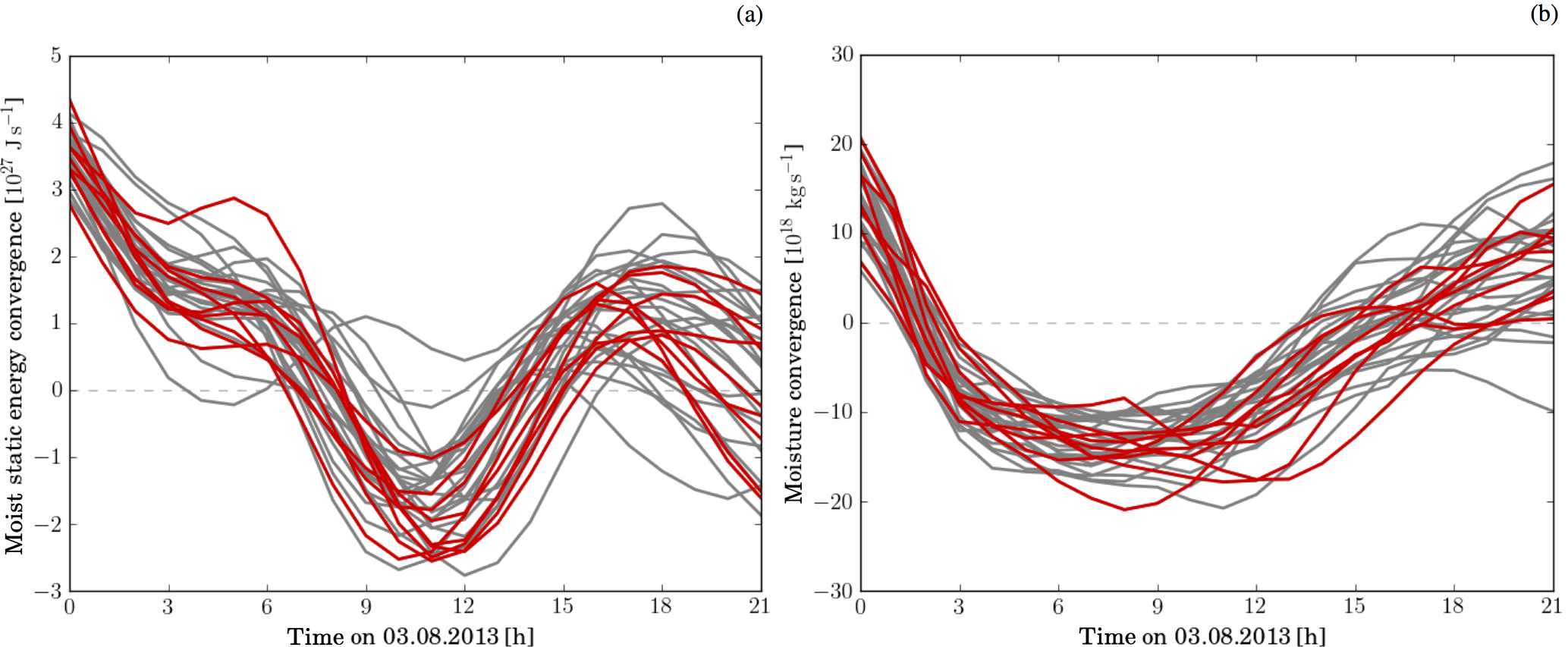
Figure 1Convergence of moist static energy (a) and moisture (b) across the 1 km domain computed from the global ensemble. The grey lines show all 33 ensemble members in the global ensemble and the red lines the 9 members selected for the regional ensemble simulations. The selection procedure is described in Sect. 2.
Regional simulations with a grid spacing of 1 km (500 by 500 grid points) are started at 00:00 UTC on 3 August 2013 from the 10 selected global model runs. These simulations provide the initial and boundary conditions for simulations in a second set of nested simulations with a horizontal grid spacing of 250 m (900 by 600 grid points). For the regional simulations, we use the UM version 10.3 (GA6 configuration, Walters et al., 2017) with the CASIM module. In contrast, to the global ensemble, we do not use the stochastic physics module for the regional ensemble, as we aim to investigate the role of initial condition uncertainty. The model set-up for the regional simulations is identical to the set-up described in Miltenberger et al. (2018). The control simulations are identical to the simulations used in Miltenberger et al. (2018), with the only difference being that the simulations discussed here use the cloud droplet number predicted by CASIM instead of a prescribed value for the computation of the radiative fluxes. Note that the aerosol direct effect is not included in the simulations. In all regional simulations, moisture conservation is enforced according to Aranami et al. (2014, 2015). All simulations are run for 24 h. If not stated otherwise, the analysis presented in this paper focusses on the time period between 09:00 and 19:00 UTC, i.e. the time period of main convective activity. Also note that ensemble members have been sorted according to the large-scale moisture convergence computed from the fluxes at the domain boundary: ensemble member 1 has the largest large-scale moisture convergence and ensemble member 9 the smallest.
Cloud microphysical processes are parameterised within the CASIM module which in this study is configured as a double-moment microphysics scheme with five different hydrometeor categories. The CASIM module can represent the interactions between aerosol fields and cloud microphysical properties. For the ensemble simulations, we use the so-called “passive-aerosols” mode: aerosol fields are used for droplet activation and ice nucleation, but are not altered by cloud microphysical processes. The impact of this choice on the representation of aerosol–cloud interactions is discussed in Miltenberger et al. (2018). Aerosol initial and lateral boundary conditions are derived from aircraft data as described in Miltenberger et al. (2018). In the following, simulations with the aerosol profile derived from observations are referred to as “standard-aerosol” simulations. Additional simulations of each ensemble member are performed with perturbed aerosol profiles, for which aerosol number densities and mass mixing ratio are multiplied at all altitudes by a factor of 10 (“high aerosol”) and 0.1 (“low aerosol”), respectively. Hence, the mean aerosol radius is retained in the perturbed profiles. Accordingly, the entire ensemble with perturbed meteorological and aerosol initial conditions has 30 members in total.
For the evaluation of the ensemble with the standard-aerosol profile, we use the same set of observations as in the first part of this study. These include radiosonde and aircraft data from the COPE field campaign and data from the operational radar network. Details about these datasets can be found in Miltenberger et al. (2018).
3.1 Radar reflectivity and surface precipitation
In all ensemble simulations, a convergence line develops roughly over the centre of the peninsula in the early afternoon (Fig. 2). The convective clouds are associated with convergence zones along sea-breeze fronts. However, the members vary in the amount of clouds and there are some differences in the location and the orientation of the main cloud line. These differences are not specific to the time instance shown in Fig. 2, but persist throughout the simulations. Differences between meteorological ensemble members are further discussed in Sect. 4, while we focus here on the comparison of the ensemble to the observational data.
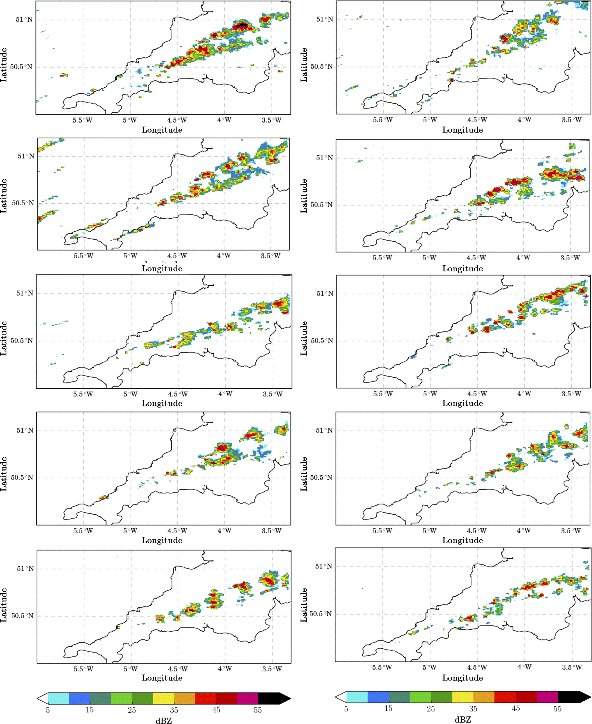
Figure 2Column maximum radar reflectivity over 250 m domain at 14:00 UTC from the control simulation (top left) and the nine ensemble members using the standard-aerosol profile.

Figure 3Comparison of domain-mean surface precipitation from model simulations and radar observations (red line). Values from the control simulation with the standard-aerosol profile are shown by the dark blue dashed line. The mean (envelope) of all ensemble members using the standard-aerosol profiles is shown by the dark blue solid line (shading) and those of all ensemble members irrespective of the used aerosol profile by the solid cyan line (shading).
Consistent with the similar meteorological evolution of the ensemble members, the domain-average precipitation has a similar temporal evolution with increasing values during the morning hours and maximum values between 13:00 and 16:00 UTC (Fig. 3). Domain-average precipitation rates from the control forecast (dashed blue line) are mostly within the spread of the ensemble members (blue shading), although the ensemble-mean domain-average precipitation rate is about a factor of 2 smaller than the control during the period of main convective activity (12:00–17:00 UTC). The spread of the ensemble including aerosol perturbations (cyan shading) is not much larger than the ensemble spread based on perturbed meteorological conditions alone, particularly after about 14:30 UTC. The ensemble mean is almost identical for both ensembles. The domain-average precipitation rates derived from radar (Radarnet IV, Harrison et al., 2009; MetOffice, 2003) fall mostly outside the spread of the ensemble. This indicates that either the ensemble is under-dispersive or that there are issues with the radar-derived surface precipitation. While the model-derived surface precipitation is the sedimentation flux at the surface, the radar-derived surface precipitation is computed from the low-level radar reflectivity according to Harrison et al. (2009). Accordingly the modelled and radar-derived surface precipitation products involve different assumptions, e.g. on sub-cloud evaporation, which has been shown to affect radar-derived surface precipitation rates (Li and Srivastava, 2001). Nevertheless, previous evaluation studies of convection-permitting ensemble simulations have also reported precipitation forecasts to be under-dispersive over longer evaluation periods (Romine et al., 2014; Schwartz et al., 2014), as not all sources of uncertainty are taken into account. For example, structural or parametric uncertainty in the model physics is not considered and perturbations to the initial and boundary conditions may not be fully representative of the true uncertainty. The incorporation of perturbations to the aerosol initial and boundary conditions does not improve the comparison. However, the under-dispersivity of the ensemble does not strongly impact the major conclusions of our study, as we interpret the meteorological uncertainty as a lower limit of meteorological variability in the discussion (Sect. 7).
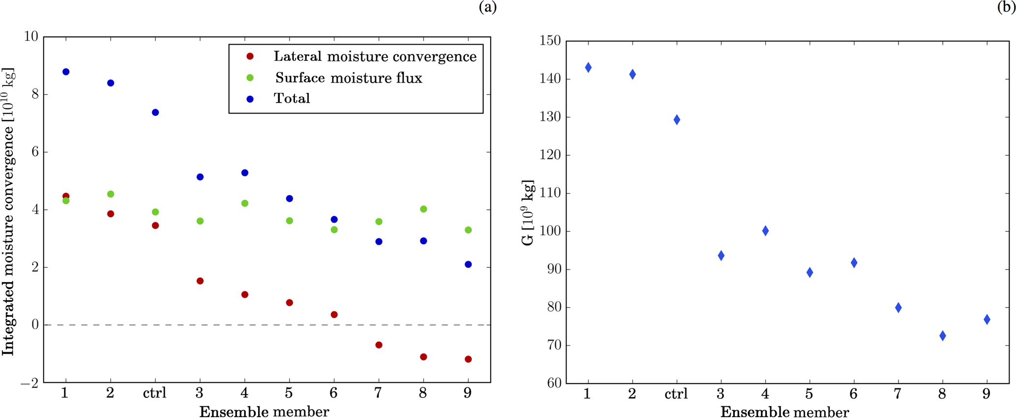
Figure 4Panel (a) shows the time-integrated net (blue), lateral (red), and surface moisture flux (green) over the model domain in the boundary layer for each ensemble member. Panel (b) shows the time-integrated condensate gain G for the different ensemble members.
The underestimation of domain-average precipitation in the ensemble is, similarly to the results in Miltenberger et al. (2018), caused by a combination of a too-small precipitating area fraction and too-low occurrence frequency of medium precipitation rates in precipitating areas (not shown). While the observed in-cloud precipitation rate distribution is outside of the ensemble spread (Fig. S1 in the Supplement), the simulated distributions of column maximum radar reflectivity and of low-level (750 m a.g.l.) radar reflectivity agree well with the observed distribution (Fig. S2). In contrast to the domain-average precipitation time series, the ensemble spread in the radar reflectivity distributions increases significantly if aerosol perturbations are considered in addition to meteorological initial condition perturbations (Fig. S2). However, the ensemble-mean distributions are almost identical for members with and without aerosol perturbations.
The 3-D radar composite available for this case provides information about the vertical structure of the clouds. Here we compare the simulated and observed altitude of the highest occurrence of a radar reflectivity larger than 18 dBZ, which is frequently used in radar products to measure cloud depth (Lakshmanan et al., 2013; Scovell and al Sakka, 2016). The ensemble mean is closer to the observed evolution than the control run (within 200 m, Fig. S3). The inclusion of perturbed aerosol initial and boundary conditions has only a small impact on the ensemble-mean height of the 18 dBZ contour (maximum difference: ±100 m). Also, for other reflectivity thresholds (5–25 dBZ), the observed mean height is within the ensemble spread and the difference to the ensemble mean is generally smaller than 500 m (not shown).
3.2 Radiosonde data
Thermodynamic profiles are available at 2-hourly intervals from radiosondes released at Davidstow (50.64∘ N, 4.61∘ W). These profiles are compared to the thermodynamic structure of the closest model grid column from the simulation with the standard-aerosol profile (Fig. S4). The overall (out of cloud) structure of the temperature and dew-point temperature profiles are similar to the observed structure for all times and ensemble members. The observed temperature profile generally falls within the ensemble spread except between 550 and 400 hPa. Also, the observed dew-point temperature profile is generally contained within the ensemble spread, with the exception of a lower observed humidity below 900 hPa at 15:20 UTC. All ensemble members have a stable layer between 5 and 6 km altitude, which is an important factor for the cloud top height distribution (Miltenberger et al., 2018). Ensemble members differ mainly in the humidity above 600 hPa, with the altitude of the driest point in this layer varying by about 100 hPa.
The height of the 0∘ level and the lifting condensation level corroborate the good agreement between observed and modelled profiles for the duration of the simulation and all aerosol scenarios: maximum deviations are about 300 m for the 0∘ level height and 400 m in the lifting condensation level (Fig. S5). While the observed lifting condensation level falls within the ensemble spread (except at 15:20 UTC), the observed 0∘ level is generally outside the ensemble spread (except at 13:50 UTC, but the radiosonde passed through clouds).
Overall the ensemble reflects the cloud and precipitation evolution, as well as thermodynamic structure indicated by observational data. However, the ensemble does not improve on the performance of the control run. Overall the ensemble performance provides confidence that the most important physical mechanisms are well enough represented to conduct aerosol perturbation experiments.
Given the overall similar meteorological situation in the ensemble members, i.e. a line of convective clouds forming along sea-breeze convergence zones, the main impact of the perturbed meteorological initial conditions should be (i) perturbations to vertical lifting and hence condensation and (ii) the vertical cloud structure by modifications to the vertical wind shear and the thermodynamic profiles. The discussion in this section focusses on the meteorological ensemble with the standard-aerosol profile. Differences in the large-scale moisture convergence, upstream thermodynamic profiles, and sea-breeze strength are discussed in Sect. 4.1. The resulting variation in cloud properties is described in Sect. 4.2.
4.1 Large-scale convergence and condensate formation
The meteorological ensemble members have been selected on the basis of the moisture and moist static energy convergence (Sect. 2), as the large-scale moisture convergence should influence the amount of lifting and hence condensate formation. The large-scale convergence is diagnosed from the moisture fluxes at the domain boundaries. Here, we focus on the boundary-layer moisture convergence, which is most relevant for the cloud-base mass flux. As expected, ensemble members have very different boundary-layer moisture convergence (Fig. 4a, red symbols). Consistent with this variability, the condensate gain G, i.e. the domain-integrated condensation and deposition rate, varies across ensemble members with decreasing values for members with smaller large-scale boundary-layer moisture convergence (Fig. 4b). The correspondence between moisture convergence and G is further improved if the net moisture flux at the top of the boundary layer is considered (Fig. 4a, blue symbols), which is diagnosed from the sum of the moisture flux at the domain boundaries (red symbols) and the surface moisture flux (green symbols). The surface moisture flux adds some modifications to the boundary-layer moisture budget, e.g. compare total and lateral moisture convergence for ensemble members 3 and 4 and member 7 and 8, respectively.
In addition to the large-scale moisture convergence, differences in meteorological initial and boundary conditions could also result in different local convergence patterns, i.e. sea-breeze strength. Differences in sea-breeze strength between ensemble members can contribute to the variability of G across the meteorological ensemble. The main controlling factors for sea-breeze strength are the temperature difference between sea and land, the large-scale wind direction relative to the coastline, and the background wind speed (Estoque, 1961; Miller et al., 2003). Golding et al. (2005) and Warren et al. (2014) have demonstrated the importance of differential heating of the land surface and the interaction with the background wind field for stationary convergence lines and associated convective activity over the southwest peninsula of the UK. The profiles of the wind components, temperature, and specific humidity are shown in Fig. S6; the variation in the land–sea temperature gradient in Fig. S7a; and the “low-level” convergence, i.e. the integrated convergence of the 10 m wind speed over the peninsula, as indicator of the sea-breeze strength in Fig. S7b.
The temperature difference between land and sea increases from 0.9–1.4 K in the morning to 1.8–2.0 K by noon. Only in ensemble members 1 and 2, the temperature difference remains smaller than 1.5 K (Fig. S7a). These members have a higher cloud fraction in the morning (not shown), which is likely related to a relatively large large-scale moisture convergence. The higher cloud fraction reduces radiative heating of the land surface explaining the smaller peak land–sea temperature difference. The wind speed in the boundary layer varies between about 8 and 11 m s−1 and increases to values of 13–18 m s−1 at 4 km altitude (Fig. S6a). The wind direction is generally from the southwest with a variability of about 10∘ and a shift towards a more easterly direction at higher altitudes (Fig. S6b).
The low-level convergence consistently increases towards noon as is expected for sea-breeze systems (Fig. S7b). Overall there are only small differences in the time-integrated low-level convergence between ensemble members. This suggests that neither the variability in the land–sea temperature difference (≈0.5 K) nor the variability in the low-level wind speed (≈3 m s−1) and direction () has a significant impact on the sea-breeze strength.
Other variables in the initial conditions important for cloud and precipitation formation are the temperature and moisture profiles (Fig. S6c and d). The temperature structure in all ensemble members is very similar, with a well-mixed boundary layer below 800 ± 200 m, an almost moist-adiabatic temperature gradient up to 500 hPa, and a layer of almost constant temperature between 500 and 450 hPa. As a result of the small variation in the temperature profile, the average and maximum CAPE values are similar for all ensemble members (100–160 J kg−1, Fig. S8). Also, variations in the moisture content are small, with difference between ensemble members smaller than 0.5 g kg−1 for all altitudes. The altitude of the driest point in the profile varies by about 100 hPa between ensemble members (Fig. S4).
4.2 Cloud property variability
The different meteorological initial and boundary conditions result in different boundary-layer moisture convergence, thermodynamic and moisture profiles, and wind shear as discussed in the previous sections. These changes can impact cloud properties, cloud field structure, and precipitation formation.
The cloud droplet number concentration (CDNC) at cloud base is almost invariant across ensemble members (Fig. 5), suggesting relatively small differences in the cloud-base vertical velocity distribution (Fig. S9b). Cloud top cloud droplet number concentrations also display little variability between meteorological ensemble members (Fig. S9a).
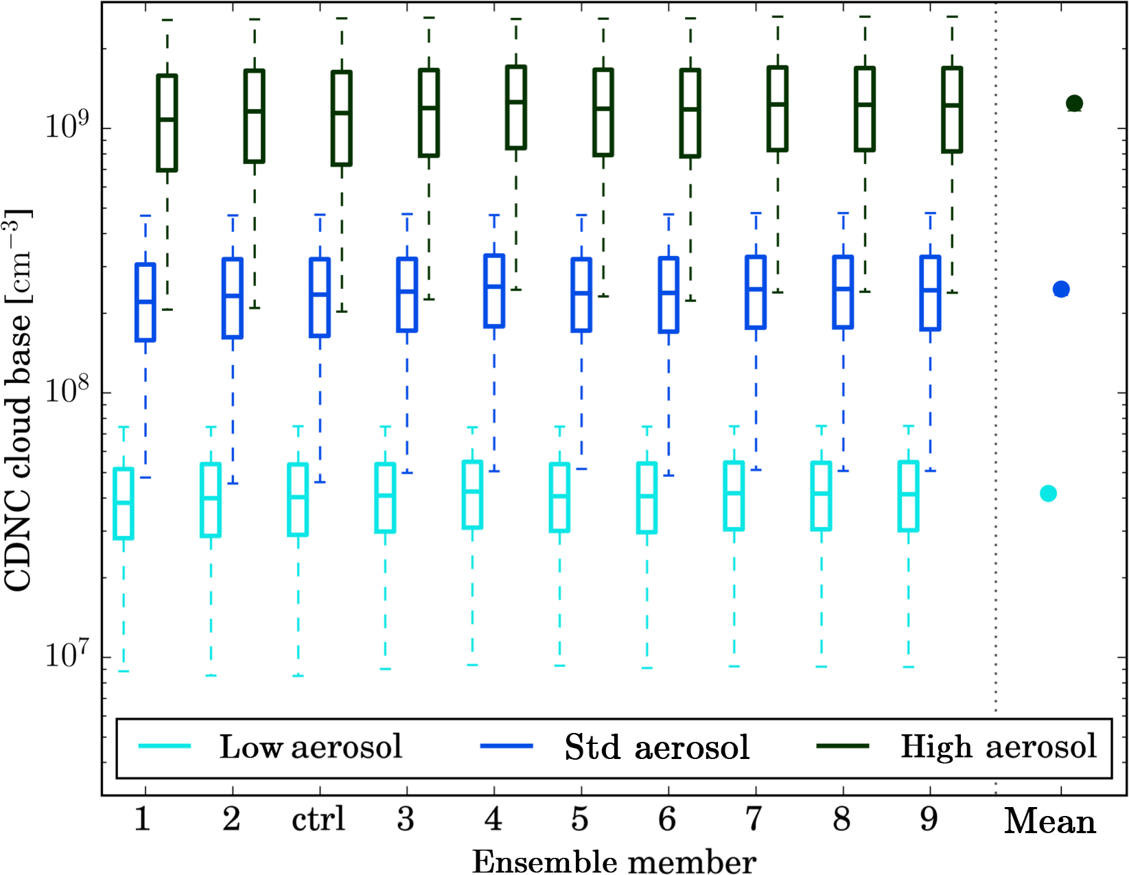
Figure 5Cloud droplet number concentration (CDNC) at cloud base for different ensemble members (abscissa) using different aerosol profiles (colours). CDNC at cloud base is computed as the average CDNC within 500 m above the lowest point in each grid column that has a cloud or ice mass mixing ratio larger than 1 mg kg−1. The horizontal line inside the boxes indicates the mean CDNC; the upper and lower edges the 25th and 75th percentile, respectively; and the whiskers the 1st and 99th percentile. The statistics are computed over all qualifying grid points in the domain between 09:00 and 19:00 UTC and therefore reflect the spatial and temporal variability of CDNC. The last column provides the distribution of the ensemble means, with the dot representing the average of the ensemble means and the bars the spread of the ensemble means.
The cloud field structure is described in terms of the cloud fraction, cell number and mean size, and cloud top height. Cells are defined as coherent areas with a column maximum radar reflectivity larger than 25 dBZ. Cloud top height is defined by the highest model level with a condensed water content larger than 1 mg kg−1 (Fridlind et al., 2010). Cloud fraction is calculated as the areal fraction of the domain with condensed water path larger than 0.001 kg m−2 (Grosvenor et al., 2017). Cell number (Fig. 6a) and cloud fraction (Fig. 7) in general decrease with decreasing boundary-layer moisture convergence and condensate gain. However, variations in mean cell size are quite small (Fig. 6b). Mean cloud top height varies by about 750 m between ensemble members (Fig. 8a), with largest (smallest) values for ensemble member 2 and 9 (5). Variations in mean cloud top height are in general consistent with those of the equilibrium level pressure (Fig. S10): for example, the equilibrium level pressure in ensemble member 5 is largest, while members 2 and 9 have the smallest equilibrium level pressure. The distribution between low, medium, and high cloud tops varies by about 20 % between the ensemble members (Fig. 8b).
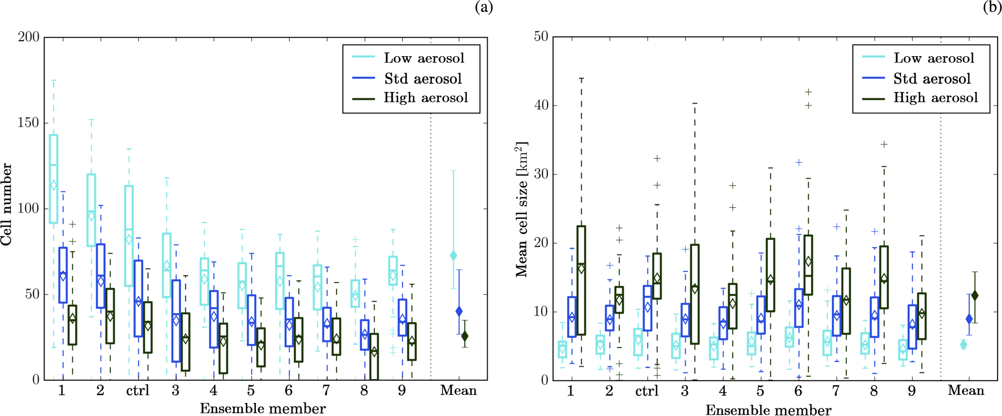
Figure 6Cell number (a) and mean cell size (b). Cells are defined as continuous areas of column maximum radar reflectivity exceeding 25 dBZ. The horizontal line inside the boxes indicates the time mean value; the upper and lower edges the 25th and 75th percentile, respectively; and the whiskers the 1st and 99th percentile. These statistics reflect the temporal variability of the considered variables. The last column in each panel provides the distribution of the ensemble means, with the dot representing the average of the ensemble means and the bars the spread of the ensemble means.
Precipitation formation is described by the condensation ratio CR and the precipitation efficiency PE. These describe the fraction of the incoming moisture flux that is converted to condensate (CR) and the fraction of the condensate gain that is converted to surface precipitation (PE). As expected, CR varies strongly across ensemble members and in general decreases with decreasing large-scale moisture convergence (Fig. 9a). In contrast, PE does not vary systematically with the large-scale convergence (Fig. 9a). Ensemble member 4 has a significantly lower PE than the other ensemble members, which is likely related to the high fraction of shallow clouds with cloud tops below 2.5 km and a therefore small contribution of mixed-phase processes to domain-wide precipitation formation. Conversely, ensemble member 6 has a relatively large PE and the largest fraction of clouds with tops above 4.3 km. The relatively small differences in precipitation efficiency (between 0.17 and 0.27) are consistent with the almost invariant cloud droplet number concentrations for all ensemble members (Fig. 5). The combined effect of CR and PE results in a variation of about a factor 1.5 in the mean precipitation rate (Fig. 10a) and the accumulated precipitation (Fig. S11a and b). The precipitation variability corresponds in general to the variations in large-scale moisture convergence with some modulations by the different precipitation efficiencies (e.g. compare ensemble member 2 and control or ensemble members 5 and 6). Variations in the mean condensed water path are consistent with variations in the condensate generation between ensemble members (Fig. 10b); i.e. the condensed water path decreases in members with smaller moisture convergence and G.
Mean reflected shortwave radiation ranges from 130 to 155 W m−2 (Fig. 11a). The reflected shortwave is influenced by the cloud cover and the cloud droplet number concentrations. The largest (smallest) outgoing shortwave flux is predicted for the ensemble members with the largest (smallest) cloud fraction, i.e. ensemble 1 (8). Since the CDNC variability is small (Fig. 5), the variations in cloud fraction between ensemble members dominate the variability of outgoing shortwave radiation (OSR). Changes in outgoing longwave radiation (OLR) are on the order of 3 W m−2 (Fig. 11b). The outgoing longwave radiation is influenced by the surface temperature, the cloud top height, and the cloud fraction. While differences in the cloud top height distribution contribute to the variability in outgoing longwave radiation, variations in the clear sky outgoing longwave radiation dominate the overall variability due to the relatively small cloud fraction (Fig. S12).
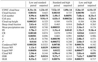
The simulation of each meteorological ensemble member was conducted with three different aerosol profiles: a so-called standard-aerosol scenario, which was derived from aircraft observations; and low- and high-aerosol scenarios, which have a factor of 10 lower and higher aerosol number concentration, respectively. The impact of the perturbed aerosol profiles on cloud and cloud field properties as well as precipitation formation in the control simulation has been discussed in the first part of this study. In this section, we compare the aerosol signal in the different meteorological ensemble members, i.e. the difference in realisations with different aerosol scenarios but identical meteorological initial and boundary conditions. Therefore, we test the robustness of aerosol-induced changes to small perturbations in the meteorological conditions. To quantify the significance of aerosol-induced changes we use a two-sided t test for ensemble members paired according to meteorological conditions (Table 1). Using paired ensemble members reflects the interdependence of cloud properties in realisations with different aerosol but identical meteorological initial and boundary conditions. Significance is tested at the 5 % level.
Table 1The p values from two-sided t tests with the null hypothesis of no change in the variable (rows) between two aerosol scenarios (columns) for all ensemble members. The results for ensemble members paired according to meteorological conditions and unpaired members are provided. Bold numbers indicate statistical significance at the 5 % level.
5.1 Cloud droplet number concentration
The cloud-base CDNC is shown in Fig. 5 for all ensemble members and aerosol profiles. All ensemble members show a consistent increase in the cloud-base CDNC by about a factor of 7 between the low (standard) and the standard (high) aerosol scenarios. Also, the aerosol-induced change in cloud top CDNC is similar in all meteorological ensemble members with a change by about a factor of 5.5 for each factor of 10 increase in the background aerosol concentrations (Fig. S9a). The small differences between ensemble members suggest only minor changes in the cloud-base vertical velocity distribution. The aerosol-induced changes in CDNC are highly significant (Table 1).
5.2 Cloud field structure
The cloud field structure is described in terms of cloud fraction, cell number and size, and cloud top height. The number of cells decreases with increasing background aerosol concentrations in all ensemble members (Fig. 6a). Conversely, the cell area increases (Fig. 6b). The changes in cell number and area largely compensate for each other, so that the cloud fraction displays little sensitivity to the aerosol scenarios with changes being smaller than 0.01 (Fig. 7). Although small, the aerosol-induced change in cloud fraction is consistent across all ensemble members. It has been hypothesised in the first part of this study that the slower conversion of condensate to precipitation in high-aerosol conditions allows clouds to grow larger and to merge with other updraft cores resulting in overall fewer, but larger clouds. Also, energetic constraints potentially limit an increase in overall lifting and cloud fraction. The changes in cell number, mean cell area, and cloud fraction are all significant for paired meteorology reflecting the consistency in the sign of the aerosol-induced changes across the ensemble members (Table 1).
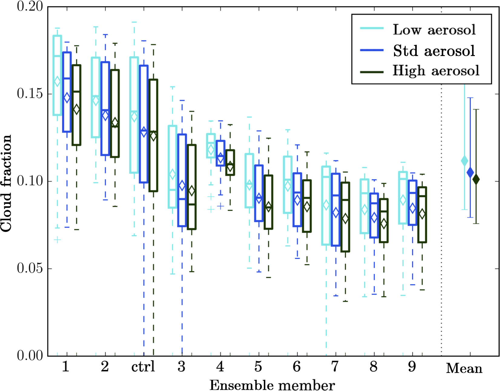
Figure 7Cloud fraction in the different ensemble members. Cloud fraction is the fraction of the domain for which the condensed water path is larger than 1 g m−2. The horizontal line inside the boxes indicates the time mean value; the upper and lower edges the 25th and 75th percentile, respectively; and the whiskers the 1st and 99th percentile. These statistics reflect the temporal variability of the considered variables. The last column in each panel provides the distribution of the ensemble means, with the dot representing the average of the ensemble means and the bars the spread of the ensemble means.

Figure 8Mean cloud top height (a) and fraction of clouds with cloud-top-specific altitude bands (b). Cloud top height is the height of the highest vertical level in each grid column with a condensate mass mixing ratio larger than 1 mg kg−1. The horizontal line inside the boxes indicates the time mean value; the upper and lower edges the 25th and 75th percentile, respectively; and the whiskers the 1st and 99th percentile. These statistics reflect the temporal variability of the considered variables. The last column in each panel provides the distribution of the ensemble means, with the dot representing the average of the ensemble means and the bars the spread of the ensemble means.
The mean cloud top height is shown in Fig. 8a and the fraction of cloud tops in different altitude ranges in Fig. 8b. In all ensemble members, the mean cloud top height increases from the low- to the standard-aerosol scenario. The increase in mean cloud top is due to an increase in the fraction of cloud tops higher than 4.3 km. In the control run and ensemble members 4 and 6, this is accompanied by a reduction in the medium altitude fraction, while in all other members changes in the low cloud top fraction dominate. For an increase in aerosol number concentration above the standard-aerosol scenario, the time-average mean cloud top height (diamonds in Fig. 8a) does not increase further (members 1 and 2) or even decreases (members 4, 5, 6, 7, 8, 9). The decrease in mean cloud top height for the latter is mainly due to an increase in the fraction of clouds with low cloud tops. The fraction of clouds with high cloud tops shows only very small changes between the simulations with standard- and high-aerosol profiles. The small change in cloud top height is likely related to the presence of a mid-tropospheric stable layer, which is present in all ensemble members and limits cloud depths (Sect. 4). Most larger convective cells have reached this “maximum” cloud top height for the standard-aerosol scenario and hence no further deepening occurs in the high-aerosol scenario. The change in cloud top height is only significant for an increase in aerosol concentrations from the low to the standard scenario, while it is not significant for a further increase in aerosol concentrations (Table 1).
5.3 Condensed water budget and precipitation formation
The condensation ratio displays only very small changes between different aerosol scenarios (Fig. 9a). Accordingly, the condensate gain G changes only by 0–4 % between the low- and the standard-aerosol scenario and by −4 % to 2.5 % between the standard- and high-aerosol scenario (Fig. S14a and b). As discussed in Miltenberger et al. (2018), the asymmetry in the response to increased and decreased aerosol concentrations is likely related to the thermodynamic limitations on cloud deepening. Changes in domain-wide condensation and deposition contribute to change in condensate gain ΔG (Fig. S14c and d). Condensation contributes most to the increases between the low- and the standard-aerosol scenario, while changes in condensation and deposition contribute about equally to ΔG between the standard- and high-aerosol scenario. Aerosol-induced modifications of CR and G are only significant for a decrease in aerosol concentrations relative to the standard scenario (Table 1).
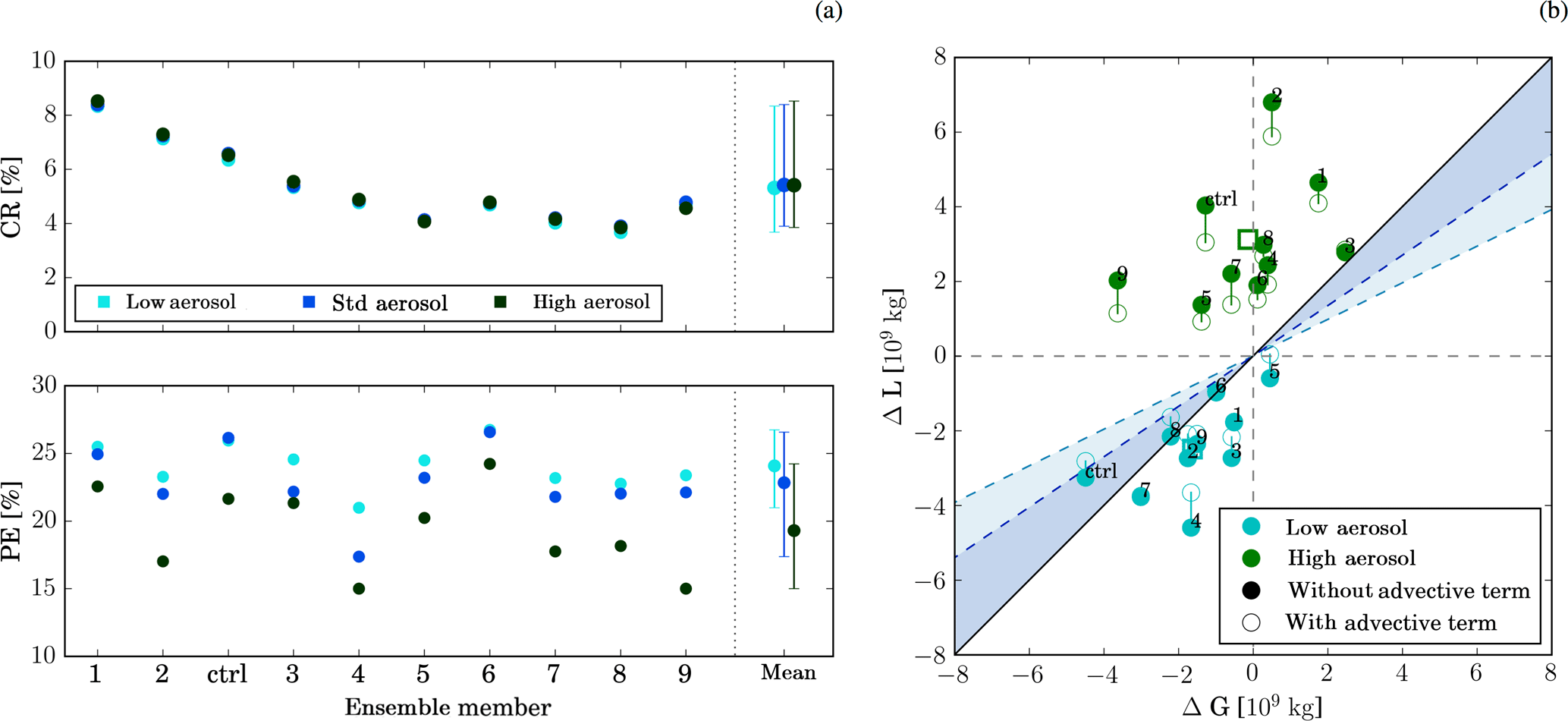
Figure 9(a) Condensation ratio and precipitation efficiency for the different ensemble members and aerosol scenarios. The last column in each panel provides the distribution of mean values from each ensemble member: the dot represents the mean over all ensemble members and the bars represent the range between the largest and smallest mean value. (b) ΔG in relation to ΔL for ensemble members paired according to the meteorological initial conditions. ΔG and ΔL are computed for simulations with the high (green symbols) and low (cyan symbols) aerosol profile relative to the simulations with the standard-aerosol profile. The filled symbols represent ΔL and ΔG values computed over the regional model domain, while the unfilled symbols include advective fluxes of condensate at the domain boundary in the loss term ΔL. The blue (cyan) shaded area indicates the region in the phase space for which changes in ΔG dominate the precipitation response using the minimum (maximum) precipitation efficiency from the ensemble with standard-aerosol conditions. The unfilled square shows the average response across the ensemble members.
The precipitation efficiency PE is more sensitive to aerosol changes than CR and decreases continuously with aerosol concentrations (Fig. 9a). The change in PE is larger for increasing than decreasing aerosol concentration relative to the standard-aerosol scenario. The stronger decrease in PE from the standard- to the high-aerosol scenario compared with the low- and standard-aerosol scenario is consistent with a higher lateral condensate transport to the stratiform region when cloud deepening becomes limited by thermodynamic constraints, as hypothesised by Miltenberger et al. (2018). With further cloud deepening limited by the upper-level stable layer, more condensate is transported into the stratiform area reducing the residence time of the condensate in the active convective core region. In contrast, cloud deepening is larger and changes in lateral condensate transport smaller when the low- and standard-aerosol scenario are compared. Therefore, the slower conversion of condensate to precipitation-sized hydrometeors in the standard-aerosol scenario can be partly balanced by a longer residence time in the convective core region. This hypothesis is discussed in more detail in Miltenberger et al. (2018). Consistent with the larger amplitude and consistent sign, the changes in PE are significant for both a decrease and an increase in aerosol concentrations relative to the standard scenario (Table 1).
The changes in the condensate budget result in a modification of the accumulated surface precipitation as illustrated in Fig. 9b. The diagram displays changes in condensate gain ΔG and condensate loss ΔL and is discussed in detail in Miltenberger et al. (2018). Increasing the aerosol concentrations from the low to the standard scenario results in a precipitation decrease in most ensemble members (points below the one-to-one line). Exceptions are the control simulation with a small increase in precipitation and ensemble members 6 and 8 with no change in accumulated surface precipitation (points on the one-to-one line). These ensemble members have a relatively small decrease in PE as well as a relatively large ΔG and G compared to ensemble members with a similar change in PE (e.g. compare ensemble member 1 and 8). Accordingly, the precipitation response in these cases is either dominated by ΔG (control) or ΔG and ΔPE are of equal importance (member 6 and 8), as also indicated by their position in the shaded area in Fig. 9b. For the other members, the change in PE dominates over changes in condensate production, as indicated by their position outside the shaded area in Fig. 9b. If the aerosol concentration is enhanced beyond the standard scenario, the precipitation decreases in all ensemble members (points above the one-to-one line). This response is dominated by PE changes in all ensemble members (points outside the shaded area). Differences in accumulated precipitation are significant, if ensemble members are paired according to meteorology (Table 1).
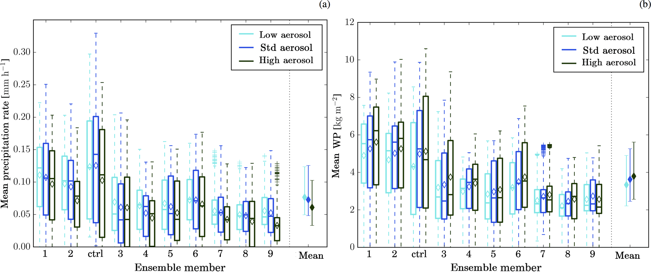
Figure 10Domain-average precipitation rate (a) and mean condensed water path (b). The horizontal line inside the boxes indicates the time mean value; the upper and lower edges the 25th and 75th percentile, respectively; and the whiskers the 1st and 99th percentile. These statistics reflect the temporal variability of the considered variables. The last column in each panel provides the distribution of the ensemble means, with the dot representing the average of the ensemble means and the bars the spread of the ensemble means.
The decrease in accumulated precipitation is accompanied by a reduced mean precipitation rate with increasing aerosol concentrations (Fig. 10a). For most ensemble members the change is larger between the standard- and high-aerosol scenario than between the standard- and low-aerosol scenario. Only in ensemble member 3 does the mean precipitation rate not decrease further in the high-aerosol scenario and in ensemble members 4 and 5 the decrease between the standard- and the high-aerosol scenario is comparable to the decrease between the low and standard scenario. The percentiles of the precipitation distribution increase for all percentiles up to and including the 75th percentile from the low to the high aerosol concentration for almost all ensemble members (Fig. S11c). The 99th percentiles are generally smallest (largest) for the high (standard) aerosol scenario. The only exception is ensemble member 4, for which the standard-aerosol scenario has the smallest 99th percentile.
The condensed water path in the domain is a result of the condensate generation and the timescale of condensate conversion to precipitation. Parcel model considerations suggest a longer timescale for precipitation formation under enhanced aerosol concentrations. Therefore, an increase in the condensed water path is expected with increasing aerosol concentrations. Indeed, the mean condensed water path in most ensemble members increases with aerosol concentrations (Fig. 10b). This is the result of small decreases in the liquid water path (cloud and rain species) and a larger gain in the mass of the frozen hydrometeors (ice, snow, and graupel species) (Fig. S13), consistent with a slower conversion of cloud droplets to rain drops and accordingly a larger mass transport across the 0 ∘C level. The only ensemble member displaying a different pattern is ensemble member 9, for which the total condensed, the solid, and the liquid water path decrease from the standard- to the high-aerosol scenario. This ensemble member has also the largest reduction in precipitation efficiency. In addition, for ensemble member 9 the mean cloud top height and the fraction of clouds with cloud tops larger than 4.3 km decrease compared to the standard-aerosol scenario. These changes are consistent with a lower condensed water path, as reduced cloud top heights indicate a smaller vertical displacement of the air parcels and accordingly less condensate generation. The decrease in precipitation efficiency is likely linked to these changes as the longer timescale for conversion of cloud droplets to precipitation-sized hydrometeors is not compensated for by a longer residence time in the cloud due the reducing vertical extent of the clouds. Aerosol-induced changes in condensed, liquid and frozen water path are significant in the paired meteorology tests (Table 1).
5.4 Radiation
The response of cloud radiative properties to changes in aerosol concentrations is climatologically important, but not well constrained, mainly due to the impact of aerosols on both cloud fraction and cloud lifetime. The reflected shortwave radiation is affected by the size and number of the hydrometeors close to cloud top and by the cloud fraction. The outgoing shortwave flux increases for higher aerosol concentrations in all ensemble members (Fig. 11a). This change is consistent with the aerosol-induced change in CDNC (Fig. 5) and the cloud albedo effect (Twomey, 1977). The co-occurring decrease in cloud fraction under high-aerosol conditions (between 2 and 9 % for a factor of 10 aerosol change) counteracts the CDNC effect, but the cloud albedo effect dominates due to the large amplitude of the CDNC change (about a factor of 7 for a factor of 10 aerosol change). Note that the radiative signal presented here does not fully take into account potential changes in radiative properties of the ice-phase species, as the effective diameter of the latter is diagnosed from the ice water content.

Figure 11Outgoing shortwave (a) and longwave (b) radiative flux at the top of the atmosphere, i.e. ≈ 40 km. The horizontal line inside the boxes indicates the time mean value; the upper and lower edges the 25th and 75th percentile, respectively; and the whiskers the 1st and 99th percentile. These statistics reflect the temporal variability of the considered variables. The last column in each panel provides the distribution of the ensemble means, with the dot representing the average of the ensemble means and the bars the spread of the ensemble means.
The outgoing longwave radiation is mainly influenced by the surface temperature, the cloud fraction, and the cloud top temperature. The mean outgoing longwave radiation shows only a small sensitivity to the aerosol scenario for all meteorological ensemble members (Fig. 11b). The small discernible trend of decreasing mean outgoing longwave radiation with increasing aerosol (< 0.5 W m−2, standard- to high-aerosol scenario) is consistent with the small increase in mean cloud top height (Fig. 8a).
Aerosol-induced modifications to the outgoing radiative fluxes are significant at the 5 % level.
In the previous two sections, the response of cloud properties to perturbations of the aerosol or meteorological initial and boundary conditions has been discussed separately. The 10 meteorological ensemble members vary in the large-scale moisture convergence, thermodynamic profile, and wind shear. The variation in the large-scale moisture convergence is most important for the cloud field properties, e.g. cloud fraction, cell number, condensate generation, and accumulated precipitation (Sect. 4). The mean cloud top height varies between ensemble members according to the different thermodynamic profiles. Aerosol-induced changes follow a similar pattern for each meteorological ensemble member (Sect. 5). An increase in aerosol number concentration translates to a larger CDNC, mean cell area, and outgoing shortwave radiation, while the cell number and precipitation efficiency decrease with increasing aerosol concentrations. The mean cloud top height, condensate generation, and outgoing longwave radiation display only very small changes in response to altered aerosol concentrations. To detect aerosol-induced changes in cloud properties or precipitation formation with observational datasets, it is important to separate changes resulting from different meteorological conditions from changes resulting from different aerosol concentrations. This is necessitated by the co-variability of aerosol and meteorological conditions in the real atmosphere. The question of the relative importance of meteorological and aerosol initial and boundary conditions for the cloud field structure and precipitation formation is also important for operational numerical weather prediction and the future design of ensemble prediction systems. Here, we use the combined meteorological and aerosol initial condition ensemble, i.e. combining the discussion of the two previous sections, to address the question of the relative importance of aerosol and meteorological variability for the COPE case. The discussion will focus on changes in the 10 h mean properties of the cloud field between 09:00 and 19:00 UTC. The mean value of the considered variable is displayed along with its spread from the meteorological ensemble members on the right side of Figs. 5–11 for each aerosol scenario (different colours). If instantaneous realisations of the different (domain-averaged) variables were to be considered (box plots on left side of the figures), the variability would be much larger than suggested by the domain-mean time-averaged plots (right side of the plots). For a quantitative assessment we use the p values from two-sided t tests for the full ensemble, i.e. not pairing ensemble members according to the meteorological initial conditions as in Sect. 4.
The cloud droplet number concentration at either cloud base or cloud top is strongly influenced by the assumed aerosol scenario but varies little between the different meteorological members (Figs. 5, S9a). As a result, a clear aerosol signal remains present even when the meteorological variability is taken into account. The aerosol-induced CDNC change remains highly significant at the 5 % level in the unpaired tests (Table 1).

Figure 12Summary of variability in time-average (09:00–19:00 UTC) cloud properties induced by variations in meteorological initial conditions (bars) and aerosol initial conditions (colours; cyan: low-aerosol scenario, blue: standard-aerosol scenario, green: high-aerosol scenario). Each variable has been normalised such that the minimum and maximum values in the entire ensemble (aerosol and meteorology) map to the value range [0, 1]. The variables displayed are cloud-base cloud droplet number CDNCcb, number of cells ncell, mean cell area acell, cloud fraction cf, mean cloud top height cth, condensation ratio CR, precipitation efficiency PE, average precipitation rate pmean, mean condensed water path WP, liquid water path LWP, mean outgoing shortwave radiation OSR, and mean outgoing longwave radiation OLR.
Although there is a stronger meteorology-induced variability in the cell number and mean cell size (Fig. 6) and the predicted range of values overlap for different aerosol scenarios, the aerosol signal is clearly detectable in these variables and aerosol effects remain significant also in the unpaired test (Table 1). However, if the cloud fraction, the mean cloud top height, or the distribution in different cloud top height classes is considered, the meteorological variability dominates (Figs. 7, 8). Hence, changes in cloud fraction, mean cloud top height, and deep cloud fraction are not significant at the 5 % level, if ensemble members are not paired according to meteorological conditions (Table 1). Considering previous arguments on convective invigoration, it is interesting to note that the cloud top height varies only very little with aerosol scenario but is sensitive to relatively small changes in meteorological conditions. Consistent with the small changes in cloud top height, no significant differences in outgoing longwave radiation exist between the aerosol scenarios (Fig. 11b, Table 1). For the outgoing shortwave radiation a stronger aerosol signal is retained above the meteorological variability due to the large impact of aerosol concentrations on CDNC (Fig. 11a). However, this signal is not statistically significant for an aerosol increase beyond the standard-aerosol scenario (Table 1).
Precipitation formation is known to be strongly influenced by dynamical and microphysical processes. Miltenberger et al. (2018) used an analysis of the water budget to separate the contributions from cloud dynamics and microphysics to aerosol-induced changes. As expected, condensation ratio CR and condensate gain G vary strongly between different meteorological ensemble members, but show little sensitivity to the aerosol scenario (Figs. 9a, S14a and b). The small dependency of the condensate gain on the aerosol number concentration may be a result of using a saturation adjustment scheme for the condensation in our model. Previous studies using a prognostic supersaturation found the condensation rates to be dependent on the CDNC number concentration (Lebo, 2014; Lebo et al., 2012; Sheffield et al., 2015). However, due to the thermodynamic constraints on integrated condensation, we do not expect this will have a strong impact on the overall behaviour of the condensate gain. In contrast to CR, the precipitation efficiency displays a relatively small systematic dependency on the large-scale moisture convergence and a large dependency on the aerosol scenario (Fig. 9a). However, the condensate loss L varies strongly across meteorological ensemble members due to its close relation with the condensation gain (Fig. S15). This co-variability is discounted for in PE. However, still only the aerosol-induced PE change between the standard- and high-aerosol scenario is significant at the 5 % level for unpaired ensemble members.
The aerosol-induced change in accumulated precipitation is the combined result of the changes in condensation ratio and precipitation efficiency. While the accumulated surface precipitation in most meteorological ensemble members decreases with increasing aerosol scenario, these differences are much smaller than the variability of accumulated surface precipitation between meteorological ensemble members (Fig. S11b). The meteorological variability is due to large differences in the condensate gain, which is directly related to the variability in large-scale moisture convergence. The aerosol signal is much larger for an increase in the aerosol concentrations beyond the standard-aerosol scenario due to a significantly larger change in the precipitation efficiency. The mean precipitation rate behaves qualitatively very similarly to the accumulated precipitation (Fig. 10a). Consistently, neither changes in mean precipitation rate nor accumulated precipitation are statistically significant (Table 1).
The ensemble-mean condensed water path increases with increasing aerosol concentrations, if all hydrometeor types are considered (Fig. 10b). However, the liquid water path (condensate in the cloud and rain category) shows relatively little sensitivity in its median value, while the mean liquid water path generally decreases with increasing aerosol concentrations (Fig. S13a). The frozen water path increases with increasing aerosol concentrations for most ensemble members (Fig. S13b), which is consistent with a longer timescale for precipitation formation. The aerosol-induced changes in both variables are much smaller than the variability induced by different meteorological initial and boundary conditions and are hence not significant at the 5 % level (Table 1).
High-resolution ensemble simulations (Δx = 250 m) with perturbed aerosol and meteorological initial and boundary conditions were performed for convection forming along sea-breeze convergence zones over the southwestern peninsula of the UK. The relative importance of perturbations in meteorological (10 members) and aerosol initial conditions (three for each member) for various cloud properties and precipitation formation is analysed over a forecast lead time of 10–20 h. The 10 different meteorological ensemble members develop similar mesoscale flow patterns with a sea-breeze convergence zone establishing over the centre of the peninsula. As a result of the different lateral boundary conditions, the large-scale boundary-layer moisture convergence and the accumulated condensate gain vary by a factor of 2 and the accumulated surface precipitation by a factor of 2.5 between ensemble members. The average cloud fraction differs by up to 0.1 between the meteorological ensemble members. This meteorological variability is compared to changes in cloud properties induced by a factor of 10 increase and decrease in aerosol number concentrations relative to the standard scenario. While the perturbations to the meteorological initial conditions reflect at best the uncertainty for the investigated case, changes in aerosol number concentration by a factor of 100 are probably even larger than what could be expected for the climatological variability.
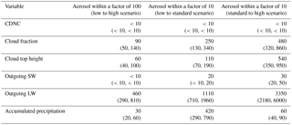
Table 2Number of observation days to obtain a statistically significant (at the 5 % level) aerosol signal in 95 % of all cases. The main value assumes the spread of the meteorological ensemble members equals 4σ, while the values in brackets use 5σ and 3σ.
Changes in aerosol concentrations can potentially modify cloud field properties, e.g. cell number and size, cloud depth, cloud fraction, and the domain-wide condensate budget (condensate gain and loss, precipitation rate). Aerosol-induced changes are consistent across the ensemble, suggesting that the physical mechanism discussed by Miltenberger et al. (2018) is robust against small changes in meteorological initial conditions. The variability of cloud field properties across the ensemble is summarised in Fig. 12. The possibility of discerning aerosol-induced differences in various cloud metrics relative to realistic meteorological variability is assessed in the following. First, the idealised situation where the meteorological initial conditions are identical for different aerosol perturbations is assessed by pairing ensemble members according to the meteorological initial conditions. This is equivalent to testing the statistical significance of the differences between realisations with different aerosol scenarios and identical meteorological initial and boundary conditions. For the paired ensemble members, a factor of 10 increase or decrease in aerosol concentrations introduces statistically significant changes (at the 5 % level) in CDNC, cloud fraction, cell number and size, outgoing shortwave radiation, instantaneous and mean precipitation rates, and precipitation efficiency (Table 1). Note that the statistical analysis is based on a very small sample, which affects the validity of several assumptions. However, since the statistical results agree qualitatively with the physical analysis, we use the significance values as a helpful diagnostic for summarising the results. Aerosol-induced changes in accumulated precipitation are only significant for an increase in aerosol concentrations beyond the standard scenario. An analysis of the condensed water budget suggests that for a decrease in aerosol concentrations, a smaller condensation ratio is balanced by an increasing precipitation efficiency. In contrast, for higher aerosol concentrations than in the standard scenario, the precipitation response is dominated by a strong decrease in precipitation efficiency with little change in the condensation ratio due to the thermodynamic constraints on cloud top height.
Secondly, we can use the simulations to assess our ability to discern aerosol–cloud effects for the situation where meteorological initial and boundary conditions are similar but subject to observational uncertainty. This would represent a “perfect” observational campaign where the meteorological conditions each day are only slightly different (convergence within a factor of 2) and large perturbations to aerosol concentrations occur (factor of 10–100). This scenario is replicated by analysing aerosol-induced changes in the full ensemble without pairing ensemble members according to meteorological initial conditions. For the unpaired ensemble, only aerosol-induced changes in CDNC, cell number and size, outgoing shortwave radiation, and precipitation efficiency are statistically significant (Table 1). For some of these variables, the changes are significant only for a decrease or an increase in aerosol number concentration relative to the standard scenario. For all other investigated variables (cloud fraction, cloud top height, condensation ratio, domain-average precipitation rate, condensed water path, and liquid water path) the variability resulting from different meteorological initial and boundary conditions is equal to or larger than the aerosol-induced changes.
The ensemble data can be used for a rough estimate of the number of observations that are required for retrieving a robust aerosol signal from observational data for sea-breeze convection. For this analysis we assume (i) the aerosol scenario and meteorology are independent, (ii) the ensemble is representative of the meteorological variability, (iii) the meteorological variability can be described by a Gaussian distribution, and (iv) observational data are perfect. While it is difficult to a priori estimate the impact of these assumptions on the analysis, we expect the analysis to provide a lower limit of the required number of observations due to the following reasons: in contrast to assumption (i), aerosol and meteorological conditions are likely to be correlated (Brenguier et al., 2003; Naud et al., 2016; Wood et al., 2017), reducing the observed section of the phase space. Secondly, the meteorological variability in the ensemble simulations is not representative of the climatological variability of meteorological conditions for sea-breeze convection over the southwestern peninsula of the UK, which can be assumed to be much larger (Golding, 2005). Lastly, observational data will not be perfect due to measurement errors and spatial and temporal sampling issues (Schutgens et al., 2017). All these issues will likely increase the number of required samples compared to the values suggested by our analysis.
With the assumptions listed above, a Gaussian distributions representing the meteorological variability is defined for the low- and the high-aerosol scenario. For each variable, the mean value across all ensemble members with the same aerosol scenario is used as the mean of the Gaussian distribution. The standard deviation σ of the Gaussian distribution is defined by assuming the value range (minimum and maximum) across the ensemble members equals 4σ (3σ and 5σ are tested as well). Then 104 realisations with n samples are drawn from the Gaussian distributions for the low- and high-aerosol scenario separately. The number of samples n can be interpreted as the number of times the same day is observed, as the statistical analysis presented here uses either daily average or accumulated variables. However, it may be possible to interpret the necessary number of observations also as number of individual observations, e.g. from satellite overpasses, if subsequent observations are not autocorrelated, i.e. are from different cloud lifecycles. If snapshots are used, it may be necessary to take into account the possibly different life cycle stages of the observed cloud field (Luo et al., 2009; Witte et al., 2014). However, given the limited number of ensemble members in our analysis, an assessment of this effect is beyond the scope of our study. For each of the 104 realisations, we test the hypothesis that the low- and high-aerosol scenarios are not equal with a two-sided t test. The resulting distribution of p values gives the probability that a significant aerosol-signal can be retrieved from a sample of n observations with low- and high-aerosol conditions each (Fig. S16). The number of days required to have a 95 % chance of observing a significant aerosol-induced change in various cloud properties is listed in Table 2. This required number of observations only gives an approximate indication, as the exact number is sensitive to the assumptions made regarding the presentation of the meteorological variability in the ensemble, e.g. whether the ensemble spread corresponds to 3σ, 4σ, or 5σ. It is important to note that the statistical analysis has the strong caveat of being based on a rather small ensemble. To obtain robust statistics a much larger ensemble with several hundreds of ensemble members would be required, which is currently beyond the computational resources available. However, we think the analysis provided here gives some general indication of the scale of observations required as the statistics confirm the impressions gained from the physical analysis of the ensemble members. Our analysis indicates that a small sample n ≤ 10 is sufficient for variables such as the CDNC and outgoing shortwave radiation, while a large sample often exceeding 100 is required for variables such as cloud fraction, cloud top height, or accumulated precipitation. The number of samples required depends on the amplitude of the aerosol perturbation (factor of 100 between low- and high-aerosol scenario, factor of 100 between the low- (high-) and the standard-aerosol scenario) as well as the location in the aerosol space (different for increase or decrease relative to the standard-aerosol scenario). In general, more observations are required for an increase in aerosol number concentrations above the standard scenario, which is related to the thermodynamic constraints on aerosol-induced changes in the considered case discussed in Miltenberger et al. (2018). The only exception is accumulated surface precipitation, for which fewer observations are required for an increase above the standard scenario. This reflects the larger aerosol-induced signal in accumulated precipitation for increased compared to decreased aerosol concentrations.
While the meteorological ensemble allows us to put the aerosol-induced changes in cloud properties into the context of changes related to meteorological variability, the considered changes in meteorology are fairly small (Sect. 4). Even if the represented meteorological variability is assumed to be representative of all possible meteorological conditions on the investigated day, they do not cover the full range of meteorological conditions that could occur for convection along sea-breeze convergence zones. However, even this very conservative estimate on the meteorological variability is for many variables on the same order of magnitude or larger than the aerosol-induced changes. We expect that the number of samples required to retrieve a statistically robust aerosol-induced change would increase if the climatological variability of the meteorological conditions is considered.
The results presented in this paper certainly only pertain to the specific cloud type investigated and the relative magnitude of aerosol- and meteorology-related changes in cloud properties may be different for other cloud types. This will be investigated in future studies. In addition to the results presented here, some previous studies have highlighted the importance of considering the intrinsic predictability of investigated cases before drawing conclusions about the significance of aerosol-induced changes in cloud properties (Grabowski et al., 1999; Khairoutdinov and Randall, 2003; Morrison, 2012; Morrison and Grabowski, 2011; Zeng et al., 2008). These studies used prescribed large-scale conditions and applied random perturbations to thermodynamic fields throughout the simulations. The present study complements their analysis by considering the impact of changes in the large-scale conditions, which are small compared to observational uncertainties and much smaller than the expected variability in meteorological categories used to retrieve aerosol signals from general circulation models (Bony et al., 2004; Zhang et al., 2016). Consistent with previous studies, we find that the aerosol signals in variables closely related to aerosol concentrations, such as cloud droplet number concentrations, are easier to retrieve than for variables that are linked to aerosol concentrations by a series of complex processes, such as accumulated surface precipitation. From the limited number of studies available, the set of variables in either category appears to vary for different cloud types and geographic location. However, our and previous studies all suggest that aerosol-induced change in surface precipitation is very difficult to retrieve reliably (Khairoutdinov and Randall, 2003; Morrison and Grabowski, 2011).
The evidence presented in the to-date very limited number of studies considering the relative impact of meteorological and aerosol conditions on cloud properties suggests that it is crucial to carefully consider intrinsic predictability, meteorological conditions, and co-variability between aerosol and meteorological conditions in modelling and observational studies of aerosol indirect effects. While these aspects have been highlighted by Stevens and Feingold (2009) and Feingold et al. (2016), only a few modelling studies have investigated these aspects and there is a clear need for future studies extending the analysis to other cloud types and meteorological scenarios. An improved knowledge and quantification of these aspects is mandatory for progress in our understanding of aerosol-induced changes in cloud properties and for retrieving observational evidence thereof.
Model data are stored on the tape archive provided by JASMIN (http://www.jasmin.ac.uk/, Centre for Environmental Data Analysis, 2018a) service. Data access to Met Office data via JASMIN is described at http://www.ceda.ac.uk/blog/access-to-the-met-office-mass-archive-on-jasmin-goes-live/ (Centre for Environmental Data Analysis, 2018b).
The supplement related to this article is available online at: https://doi.org/10.5194/acp-18-10593-2018-supplement.
All authors contributed to the development of the concepts and ideas presented in this paper. BJS developed the CASIM microphysics code. AAH, JMW, PRF, and AKM contributed to the further development of the CASIM code. AKM and PRF set up the model runs. AKM performed the model simulations and analysis and wrote the majority of the manuscript, along with input and comments from all co-authors.
The authors declare that they have no conflict of interest.
We thank the COPE research team for collecting observational data, Alan Blyth
for very useful discussion input, and Jill Johnson for the insightful
discussions on the statistical analysis. We acknowledge use of the
Monsoon/NEXCS system, a collaborative facility supplied under the Joint
Weather and Climate Research Programme, a strategic partnership between the
Met Office and the Natural Environment Research Council. Furthermore, we
acknowledge JASMIN storage facilities (https://doi.org/10.1109/BigData.2013.6691556) as
well as FAAM, CEDA, BADC, and the Met Office for providing data. Funding for
this study has been provided by the University of Leeds and the UK Natural
Environment Research Council under grant NE/J023507/1. We thank two anonymous
reviewers for their valuable feedback.
Edited
by: Johannes Quaas
Reviewed by: two anonymous referees
Altaratz, O., Koren, I., Remer, L. A., and Hirsch, E.: Review: Cloud invigoration by aerosols – coupling between microphysics and dynamics, Atmos. Res., 140–141, 38–60, https://doi.org/10.1016/j.atmosres.2014.01.009, 2014. a
Aranami, K., Zerroukat, M., and Wood, N.: Mixing properties of SLICE and other mass-conservative semi-Lagrangian schemes, Q. J. Roy. Meteor. Soc., 140, 2084–2089, https://doi.org/10.1002/qj.2268, 2014. a
Aranami, K., Davies, T., and Wood, N.: A mass restoration scheme for limited-area models with semi-Lagrangian advection, Q. J. Roy. Meteor. Soc., 141, 1795–1803, https://doi.org/10.1002/qj.2482, 2015. a
Beck, J., Bouttier, F., Wiegand, L., Gebhardt, C., Eagle, C., and Roberts, N.: Development and verification of two convection-allowing multi-model ensembles over Western Europe, Q. J. Roy. Meteor. Soc., 142, 2808–2826, https://doi.org/10.1002/qj.2870, 2016. a
Berner, J., Ha, S.-Y., Hacker, J. P., Fournier, A., and Snyder, C.: Model uncertainty in a mesoscale ensemble prediction system: stochastic versus multiphysics representations, Mon. Weather Rev., 139, 1972–1995, https://doi.org/10.1175/2010MWR3595.1, 2011. a
Blyth, A. M., Bennett, L. J., and Collier, C. G.: High-resolution observations of precipitation from cumulonimbus clouds, Meteorol. Appl., 22, 75–89, https://doi.org/10.1002/met.1492, 2015. a
Bony, S., Dufresne, J. L., Le Treut, H., Morcrette, J. J., and Senior, C.: On dynamic and thermodynamic components of cloud changes, Clim. Dynam., 22, 71–86, https://doi.org/10.1007/s00382-003-0369-6, 2004. a
Bowler, N. E., Arribas, A., Mylne, K. R., Robertson, K. B., and Beare, S. E.: The MOGREPS short-range ensemble prediction system, Q. J. Roy. Meteor. Soc., 134, 703–722, https://doi.org/10.1002/qj.234, 2008. a, b
Bowler, N. E., Arribas, A., Beare, S. E., Mylne, K. R., and Shutts, G. J.: The local ETKF and SKEB: upgrades to the MOGREPS short-range ensemble prediction system, Q. J. Roy. Meteor. Soc., 135, 767–776, https://doi.org/10.1002/qj.394, 2009. a
Brenguier, J.-L., Pawlowska, H., and Schüller, L.: Cloud microphysical and radiative properties for parameterization and satellite monitoring of the indirect effect of aerosol on climate, J. Geophys. Res., 108, 8632, https://doi.org/10.1029/2002JD002682, 2003. a
Centre for Environmental Data Analysis: Jasmin system, available at: http://www.jasmin.ac.uk/, last access: July 2018a. a
Centre for Environmental Data Analysis: Access to MetOffice data on the jasmin system, available at: http://www.ceda.ac.uk/blog/access-to-the-met-office-mass-archive-on-jasmin-goes-live/, last access: July 2018b. a
Devasthale, A., Kruger, O., and Grassl, H.: Change in cloud-top temperatures over Europe, IEEE Geosci. Remote S., 2, 333–336, https://doi.org/10.1109/LGRS.2005.851736, 2005. a
Estoque, M. A.: A theoretical investigation of the sea breeze, Q. J. Roy. Meteor. Soc., 87, 136–146, https://doi.org/10.1002/qj.49708737203, 1961. a
Fan, J., Wang, Y., Rosenfeld, D., and Liu, X.: Review of Aerosol–Cloud Interactions: Mechanisms, Significance, and Challenges, J. Atmos. Sci., 73, 4221–4252, https://doi.org/10.1175/JAS-D-16-0037.1, 2016. a
Feingold, G., McComiskey, A., Yamaguchi, T., Johnson, J. S., Carslaw, K. S., and Schmidt, K. S.: New approaches to quantifying aerosol influence on the cloud radiative effect, P. Natl. Acad. Sci. USA, 113, 5812–5819, https://doi.org/10.1073/pnas.1514035112, 2016. a
Fridlind, A. M., Ackerman, A. S., Petch, J., Field, P. R., Hill, A., McFarquhar, G., Xie, S., and Zhang, M.: ARM/GCSS/SPARC TWP-ICE CRM intercomparison study, NASA Tech. Memo., NASA TM-2010-215858, 24 pp., 2010. a
Golding, B.: Boscastle and North Cornwall post flood event study – meteorological analysis of the conditions leading to flooding on 16 August 2004, Forecasting Research Technical Report 459, Met Office, 2005. a
Golding, B., Clark, P., and May, B.: The Boscastle flood: Meteorological analysis of the conditions leading to flooding on 16 August 2004, Weather, 60, 230–235, https://doi.org/10.1256/wea.71.05, 2005. a
Grabowski, W. W.: Indirect impact of atmospheric aerosols in idealised simulations of convective-radiative equilibrium, J. Climate, 19, 4664–4682, https://doi.org/10.1175/JCLI3857.1, 2006. a
Grabowski, W. W., Wu, X., and Moncrieff, M. W.: Cloud Resolving Modeling of Tropical Cloud Systems during Phase III of GATE. Part III: Effects of Cloud Microphysics, J. Atmos. Sci., 56, 2384–2402, https://doi.org/10.1175/1520-0469(1999)056<2384:CRMOTC>2.0.CO;2, 1999. a, b, c, d
Grosvenor, D. P., Field, P. R., Hill, A. A., and Shipway, B. J.: The relative importance of macrophysical and cloud albedo changes for aerosol-induced radiative effects in closed-cell stratocumulus: insight from the modelling of a case study, Atmos. Chem. Phys., 17, 5155–5183, https://doi.org/10.5194/acp-17-5155-2017, 2017. a, b
Gryspeerdt, E., Stier, P., and Partridge, D. G.: Links between satellite-retrieved aerosol and precipitation, Atmos. Chem. Phys., 14, 9677–9694, https://doi.org/10.5194/acp-14-9677-2014, 2014. a, b
Harrison, D. L., Scovell, R. W., and Kitchen, M.: High-resolution precipitation estimates for hydrological uses, P. I. Civil Eng.-Water, 162, 125–135, https://doi.org/10.1680/wama.2009.162.2.125, 2009. a, b
Hill, A. A., Shipway, B. J., and Boutle, I. A.: How sensitive are aerosol-precipitation interactions to the warm rain representation?, J. Adv. Model. Earth Sy., 7, 987–1004, https://doi.org/10.1002/2014ms000422, 2015. a
Khairoutdinov, M. F. and Randall, D. A.: Cloud Resolving Modeling of the ARM Summer 1997 IOP: Model Formulation, Results, Uncertainties, and Sensitivities, J. Atmos. Sci., 60, 607–625, https://doi.org/10.1175/1520-0469(2003)060<0607:CRMOTA>2.0.CO;2, 2003. a, b, c, d
Koren, I., Feingold, G., and Remer, L. A.: The invigoration of deep convective clouds over the Atlantic: aerosol effect, meteorology or retrieval artifact?, Atmos. Chem. Phys., 10, 8855–8872, https://doi.org/10.5194/acp-10-8855-2010, 2010. a
Lakshmanan, V., Hondl, K., Potvin, C. K., and Preignitz, D.: An improved method for estimating radar echo-top height, Weather Forecast., 28, 481–488, https://doi.org/10.1175/WAF-D-12-00084.1, 2013. a
Lebo, Z. J.: The Sensitivity of a Numerically Simulated Idealized Squall Line to the Vertical Distribution of Aerosols, J. Atmos. Sci., 71, 4581–4596, https://doi.org/10.1175/JAS-D-14-0068.1, 2014. a
Lebo, Z. J., Morrison, H., and Seinfeld, J. H.: Are simulated aerosol-induced effects on deep convective clouds strongly dependent on saturation adjustment?, Atmos. Chem. Phys., 12, 9941–9964, https://doi.org/10.5194/acp-12-9941-2012, 2012. a
Lee, S. S.: Effect of Aerosol on Circulations and Precipitation in Deep Convective Clouds, J. Atmos. Sci., 69, 1957–1974, https://doi.org/10.1175/JAS-D-11-0111.1, 2012. a, b
Leon, D. C., French, J. R., Lasher-Trapp, S., Blyth, A. M., Abel, S. J., Ballard, S., Barrett, A., Bennett, L. J., Bower, K., Brooks, B., Brown, P., Charlton-Perez, C., Choularton, T., Clark, P., Collier, C., Crosier, J., Cui, Z., Dey, S., Dufton, D., Eagle, C., Flynn, M. J., Gallagher, M., Halliwell, C., Hanley, K., Hawkness-Smith, L., Huang, Y., Kelly, G., Kitchen, M., Korolev, A., Lean, H., Liu, Z., Marsham, J., Moser, D., Nicol, J., Norton, E. G., Plummer, D., Price, J., Ricketts, H., Roberts, N., Rosenberg, P. D., Simonin, D., Taylor, J. W., Warren, R., Williams, P. I., and Young, G.: The Convective Precipitation Experiment (COPE): Investigating the origins of heavy precipitation in the southwestern United Kingdom, B. Am. Meteorol. Soc., 97, 1003–1020, https://doi.org/10.1175/BAMS-D-14-00157.1, 2016. a
Li, X. and Srivastava, R. C.: An Analytical Solution for Raindrop Evaporation and Its Application to Radar Rainfall Measurements, J. Appl. Meteorol., 40, 1607–1616, https://doi.org/10.1175/1520-0450(2001)040<1607:AASFRE>2.0.CO;2, 2001. a
Luo, Z., Liu, G. Y., Stephens, G. L., and Johnson, R. H.: Terminal versus transient cumulus congestus: A CloudSat perspective, Geophys. Res. Lett., 36, L05808, https://doi.org/10.1029/2008GL036927, 2009. a
Marsigli, C., Montani, A., and Paccagnella, T.: Perturbation of initial and boundary conditions for a limited-area ensemble: multi-model versus single-model approach, Q. J. Roy. Meteor. Soc., 140, 197–208, https://doi.org/10.1002/qj.2128, 2014. a
MetOffice: 1 km Resolution UK Composite Rainfall Data from the Met Office Nimrod System. NCAS British Atmospheric Data Centre, available at: http://catalogue.ceda.ac.uk/uuid/27dd6ffba67f667a18c62de5c3456350 (last access: June 2017), 2003. a
Miller, S. T. K., Keim, B. D., Talbot, R. W., and Mao, H.: Sea breeze: Structure, forecasting, and impacts, Rev. Geophys., 41, 1011, https://doi.org/10.1029/2003RG000124, 2003. a
Miltenberger, A. K., Field, P. R., Hill, A. A., Rosenberg, P., Shipway, B. J., Wilkinson, J. M., Scovell, R., and Blyth, A. M.: Aerosol–cloud interactions in mixed-phase convective clouds – Part 1: Aerosol perturbations, Atmos. Chem. Phys., 18, 3119–3145, https://doi.org/10.5194/acp-18-3119-2018, 2018. a, b, c, d, e, f, g, h, i, j, k, l, m, n, o, p, q, r
Morrison, H.: On the robustness of aerosol effects on an idealized supercell storm simulated with a cloud system-resolving model, Atmos. Chem. Phys., 12, 7689–7705, https://doi.org/10.5194/acp-12-7689-2012, 2012. a, b
Morrison, H. and Grabowski, W. W.: Cloud-system resolving model simulations of aerosol indirect effects on tropical deep convection and its thermodynamic environment, Atmos. Chem. Phys., 11, 10503–10523, https://doi.org/10.5194/acp-11-10503-2011, 2011. a, b, c, d
Naud, C. M., Posselt, D. J., and van den Heever, S. C.: Aerosol optical depth distribution in extratropical cyclones over the northern hemisphere oceans, Geophys. Res. Lett., 43, 10504–10511, https://doi.org/10.1002/2016GL070953, 2016. a
Romine, G. S., Schwartz, C. S., Berner, J., Fossell, K. R., Snyder, C., Anderson, J. L., and Weisman, M. L.: Representing Forecast Error in a Convection-Permitting Ensemble System, Mon. Weather Rev., 142, 4519–4541, https://doi.org/10.1175/MWR-D-14-00100.1, 2014. a, b
Rosenfeld, D., Lohmann, U., Raga, G. B., O'Dowd, C. D., Kulmala, M., Fuzzi, S., Reissell, A., and Andreae, M. O.: Flood or drought: How do aerosols affect precipitation?, Science, 321, 1309–1313, https://doi.org/10.1126/science.1160606, 2008. a
Rosenfeld, D., Andreae, M. O., Asmi, A., Chin, M., de Leeuw, G., Donovan, D. P., Kahn, R., Kinne, S., Kivekäs, N., Kulmala, M., Lau, W., Schmidt, K. S., Suni, T., Wagner, T., Wild, M., and Quaas, J.: Global observations of aerosol-cloud-precipitation climate interactions, Rev. Geophys., 52, 750–808, https://doi.org/10.1002/2013RG000441, 2014. a
Saito, K., Hara, M., Kunii, M., Seko, H., and Yamaguchi, M.: Comparison of initial perturbation methods for the mesoscale ensemble prediction system of the Meteorological Research Institute for the WWRP Beijing 2008 Olympics Research and Development Project (B08RDP), Tellus A, 63, 445–467, https://doi.org/10.1111/j.1600-0870.2010.00509.x, 2011. a
Schutgens, N., Tsyro, S., Gryspeerdt, E., Goto, D., Weigum, N., Schulz, M., and Stier, P.: On the spatio-temporal representativeness of observations, Atmos. Chem. Phys., 17, 9761–9780, https://doi.org/10.5194/acp-17-9761-2017, 2017. a
Schwartz, C. S., Romine, G. S., Smith, K. R., and Weisman, M. L.: Characterizing and Optimizing Precipitation Forecasts from a Convection-Permitting Ensemble Initialized by a Mesoscale Ensemble Kalman Filter, Weather Forecast., 29, 1295–1318, https://doi.org/10.1175/WAF-D-13-00145.1, 2014. a, b
Scovell, R. and al Sakka, H.: A point cloud method for retrieval of high-resolution 3D gridded reflectivity from weather radar networks for air traffic management, J. Atmos. Ocean Tech., 33, 461–479, https://doi.org/10.1175/JTECH-D-15-0051.1, 2016. a
Seifert, A., Köhler, C., and Beheng, K. D.: Aerosol-cloud-precipitation effects over Germany as simulated by a convective-scale numerical weather prediction model, Atmos. Chem. Phys., 12, 709–725, https://doi.org/10.5194/acp-12-709-2012, 2012. a, b, c
Sena, E. T., McComiskey, A., and Feingold, G.: A long-term study of aerosol–cloud interactions and their radiative effect at the Southern Great Plains using ground-based measurements, Atmos. Chem. Phys., 16, 11301–11318, https://doi.org/10.5194/acp-16-11301-2016, 2016. a
Sheffield, A. M., Saleeby, S. M., and van den Heever, S. C.: Aerosol-induced mechanisms for cumulus congestus growth, J. Geophys. Res.-Atmos., 120, 8941–8952, https://doi.org/10.1002/2015JD023743, 2015. a
Shipway, B. J. and Hill, A. A.: Diagnosis of systematic differences between multiple parametrizations of warm rain microphysics using a kinematic framework, Q. J. Roy. Meteor. Soc., 138, 2196–2211, https://doi.org/10.1002/qj.1913, 2012. a
Stevens, B. and Feingold, G.: Untangling aerosol effects on clouds and precipitation in a buffered system, Nature, 461, 607–613, https://doi.org/10.1038/nature08281, 2009. a, b
Tao, W.-K., Chen, J.-P., Li, Z., Wang, C., and Zhang, C.: Impact of aerosols on convective clouds and precipitation, Rev. Geophys., 50, RG2001, https://doi.org/10.1029/2011RG000369, 2012. a
Twomey, S.: The influence of pollution on the shortwave albedo of clouds, J. Atmos. Sci., 34, 1149–1152, https://doi.org/10.1175/1520-0469(1977)034<1149:TIOPOT>2.0.CO;2, 1977. a
van den Heever, S. C., Stephens, G. L., and Wood, N. B.: Aerosol indirect effect on tropical convective characteristics under conditions of radiative-convective equilibrium, J. Atmos. Sci., 68, 699–718, 2011. a
Walters, D., Baran, A., Boutle, I., Brooks, M., Earnshaw, P., Edwards, J., Furtado, K., Hill, P., Lock, A., Manners, J., Morcrette, C., Mulcahy, J., Sanchez, C., Smith, C., Stratton, R., Tennant, W., Tomassini, L., Van Weverberg, K., Vosper, S., Willett, M., Browse, J., Bushell, A., Dalvi, M., Essery, R., Gedney, N., Hardiman, S., Johnson, B., Johnson, C., Jones, A., Mann, G., Milton, S., Rumbold, H., Sellar, A., Ujiie, M., Whitall, M., Williams, K., and Zerroukat, M.: The Met Office Unified Model Global Atmosphere 7.0/7.1 and JULES Global Land 7.0 configurations, Geosci. Model Dev. Discuss., https://doi.org/10.5194/gmd-2017-291, in review, 2017. a
Wang, H., Augligné, T., and Morrison, H.: Impact of microphysics scheme complexity on the propagation of initial perturbations, Mon. Weather Rev., 140, 2287–2296, https://doi.org/10.1175/MWR-D-12-00005.1, 2012. a
Ward, J. H.: Hierarchical Grouping to Optimize an Objective Function, J. Am. Stat. Assoc., 58, 236–244, 1963. a
Warren, R. A., Kirshbaum, D. J., Plant, R. S., and Lean, H. W.: A “Boscastle-type” quasi-stationary convective system over the UK Southwest Peninsula, Q. J. Roy. Meteor. Soc., 140, 240–257, https://doi.org/10.1002/qj.2124, 2014. a
Witte, M. K., Chuang, P. Y., and Feingold, G.: On clocks and clouds, Atmos. Chem. Phys., 14, 6729–6738, https://doi.org/10.5194/acp-14-6729-2014, 2014. a
Wood, R., Stemmler, J. D., Rémillard, J., and Jefferson, A.: Low-CCN concentration air masses over the eastern North Atlantic: Seasonality, meteorology, and drivers, J. Geophys. Res., 122, 1203–1223, https://doi.org/10.1002/2016JD025557, 2017. a
Zeng, X., Tao, W.-K., Lang, S., Hou, A. Y., Zhang, M., and Simpson, J.: On the sensitivity of atmospheric ensembles to cloud microphysics in long-term cloud-resolving model simulations, J. Meteor. Soc. Jpn., 86A, 45–65, https://doi.org/10.2151/jmsj.86A.45, 2008. a, b
Zhang, S., Wang, M., Ghan, S. J., Ding, A., Wang, H., Zhang, K., Neubauer, D., Lohmann, U., Ferrachat, S., Takeamura, T., Gettelman, A., Morrison, H., Lee, Y., Shindell, D. T., Partridge, D. G., Stier, P., Kipling, Z., and Fu, C.: On the characteristics of aerosol indirect effect based on dynamic regimes in global climate models, Atmos. Chem. Phys., 16, 2765–2783, https://doi.org/10.5194/acp-16-2765-2016, 2016. a
- Abstract
- Introduction
- Model and data
- Evaluation of ensemble simulations
- Cloud property variability in the meteorological ensemble (standard-aerosol scenario only)
- Cloud property changes between ensemble members with different aerosol and identical meteorological initial and boundary conditions
- Contribution of aerosol and meteorology perturbations to overall cloud property variability
- Discussion and conclusions
- Data availability
- Author contributions
- Competing interests
- Acknowledgements
- References
- Supplement