Leveraging TROPOMI observations and WRF-GHG modeling towards improving methane emission assessments in India

Atmospheric methane (CH₄) contributes to global warming and climate change. Multiple factors control its atmospheric growth rate, posing challenges for climate change mitigation in regions with limited observations, like India. In this study, we examine the potential of dry air column methane mixing ratio (XCH₄) observations from the TROPOspheric Monitoring Instrument (TROPOMI) in conjunction with the high-resolution Weather Research and Forecasting model with Greenhouse Gas module (WRF-GHG) to improve the annual CH₄ budget of India. In addition to an inversion framework, we present a spatiotemporal assessment of bottom-up Indian methane emissions and their influence on XCH₄, supplying the context needed for regional emission optimization. Our analysis demonstrates the potential of WRF-GHG to represent the atmospheric XCH₄ and CH₄ distributions, including seasonal patterns, albeit with non-negligible uncertainties when compared with satellite and ground-based observations for 2018 and 2019. We find that the WRF-GHG simulations tend to overestimate XCH₄ while underestimating near-surface CH₄ concentrations at the Thumba site. Our inversion analyses report annual CH₄ emissions ranging from 21.9 to 24.9 Tg with an uncertainty of 3.3 Tg (anthropogenic sources), implying an overestimation of 13 % to 24 % by the EDGAR global inventory. Also, our estimates are approximately 19 % higher than those in the India Fourth Biennial Update Report (19.6 Tg) and close to the latest Global Methane Budget 2000–2020. Overall, this study demonstrates the usefulness of TROPOMI observations for assessing Indian CH₄ emissions and shows a way to improve our understanding of how regional processes can modulate atmospheric CH₄ mixing ratios. We highlight the need for expanded observational coverage and an improved carbon assimilation system over India to refine the methane budget in support of global climate goals.

1 Introduction

The concentration of atmospheric CO₂ has increased by more than 50 % of the pre-industrial levels, while that of CH₄ has increased by 150 % (Friedlingstein et al., 2025; Saunois et al., 2025). CH₄ is the most prevalent non-CO₂ greenhouse gas, with a warming potential 28 times that of CO₂ over 100 years and 84 times over 20 years. (Calvin et al., 2023; Montzka et al., 2011; Saunois et al., 2016; IPCC, 2014) and an atmospheric lifetime of 9.1 ± 0.9 years (Zhou et al., 2023; Saunois et al., 2025). Starting from 2007, the concentration of CH₄ has proliferated from an annual global mean of 1775 to 1921 ppb in 2024, with a total rise of 146 ppb, which denotes a huge overall growth since the start of industrialization. The warming of wetlands, an increase in the ruminant population, and a decline in biomass burning, previously masking the rise in isotopically negative fuel use, are some of the key factors that may have contributed to the recent surge in CH₄ concentrations (Nisbet et al., 2019). The observed decline in carbon isotope ratio (δ¹³CH₄) indicates a shift toward increasing biogenic CH₄ sources, such as microbial emissions from wetlands and agriculture (has a more negative δ¹³CH₄ signature) rather than fossil fuel or biomass burning contributions (Skeie et al., 2023; Schaefer et al., 2016). The long-term trend in OH remains uncertain, with some studies suggesting increases (e.g. Stevenson et al., 2020), others finding no significant trend (Thompson et al., 2024), and still others showing diverging results depending on methodology (Saunois et al., 2025).

The global stock-take under Article 14 of the Paris Agreement implies the responsibility of each party to prepare, communicate, and maintain the successive nationally determined contributions (NDCs) to climate action. A 30 % global reduction in CH₄ emissions from 2020 to 2030 has been aimed at the Global Methane Pledge, launched at a 2021 meeting of the United Nations Framework Convention on Climate Change (UNFCCC). Being one of the significant contributors to greenhouse gas (GHG) emissions, India plays an essential role in the global GHG scenario. Still, it lacks sufficient long-term, continuous, and accurate observations of the GHG to quantify the sources and sinks (Zhang et al., 2014). The country has the largest cattle (including bovine) population in the world (Robinson et al., 2014). Along with this, its huge intense flood irrigation practices, ever-increasing fuel demand, and large wetland extent (nearly 4.7 % of its total geographical area) contribute to its high CH₄ emission potential (Ganesan et al., 2017; Garg et al., 2011; Ministry of Environment and Change, 2015; Myhre et al., 2013b). CH₄ emissions from enteric fermentation account for about 44 % of the total CH₄ emissions of India's National GHG inventory 2020 (MoEFCC, 2024). The Emissions Database for Global Atmospheric Research (EDGAR) inventory provides a global sector-wise emission estimate for CH₄. However, the bottom-up approach of EDGAR inventory is limited by its accuracy and temporal resolution owing to uncertainties in the data used and methodologies (e.g. uncertain emission factors, aggregation or interpolation errors and sector distribution). Besides, Indian wetland emissions also show inconsistency in estimations (∼ 5 % to 9 %) depending on the wetland model used (Bloom et al., 2017). Janardanan et al. (2024) reported large uncertainty in wetland emission inventory data over the Indian domain based on satellite observations and models. Further, insufficient coverage of highly precise and accurate ground-based observations of CH₄ and inadequate access to emission reporting over the country can lead to misrepresentations in global emission inventories.

Atmospheric concentration measurements contain integrated information on the underlying source-sink distribution. Therefore, integrating atmospheric mixing ratio measurements, flux information from bottom-up approaches, and transport model simulations can potentially enhance CH₄ estimates through inverse modeling (Bergamaschi et al., 2018) and independently evaluate reported flux estimates. Previous studies over India have been limited by coarse model resolution, incomplete representation of transport processes, or lack of high-resolution emission inventories. Due to these inadequate modeling systems and sparse ground measurements, limited studies have used atmospheric CH₄ observations to inform about CH₄ emission flux estimates across India. There is an urgent call for measurement that can sufficiently constrain regional emissions in modeling systems (Patra et al., 2016). Recent technological advancements in satellite remote-sensing enable high-resolution-high-density observations to be utilized for this inverse-based quantification when modeling techniques are adequately advanced (Myhre et al., 2013a; Jacob et al., 2016; Alexe et al., 2015; Buchwitz et al., 2017; Liang et al., 2023; Lu et al., 2022). Ganesan et al. (2017) used a top-down approach to estimate India's CH₄ emission for 2010–2015. The above study used column-averaged observations of CH₄ from the Greenhouse Gases Observing Satellite (GOSAT) along with aircraft observations from Civil Aircraft for the Regular Investigation of the Atmosphere Based on an Instrument Container (CARIBIC) and a few surface measurements from Indian sites to calculate methane emissions by atmospheric inverse modeling. Since 2009, GOSAT has measured the atmospheric column for CH₄ every three days at a 10 km diameter circle (Butz et al., 2011). Despite some limitations in temporal coverage, the spatial resolution of GOSAT observations is much better than its predecessor, the Scanning Imaging Absorption Spectrometer for Atmospheric Chartography (SCIAMACHY), which the research community has widely used (Butz et al., 2011; Yokota et al., 2009; Turner et al., 2015; Buchwitz et al., 2005; Schneising et al., 2011).

Since November 2017, the more recent TROPOspheric Monitoring Instrument (TROPOMI) on board the Copernicus Sentinel-5 Precursor satellite provides much higher-density CH₄ observations at a high spatial resolution of 7 × 7 km², upgraded to 5.5 × 7 km² in August 2019 (Hu et al., 2018; Schneising et al., 2023). TROPOMI measures CH₄ at the 2.3 µm band, with a swath width of 2600 km (Jacob et al., 2016; Cusworth et al., 2018). These observations are expected to capture seasonal fluctuations, which, in turn, will give better insight into the source-sink characteristics and quantification. Hence, in the present study, we explore the potential of TROPOMI measurements in representing the distribution of CH₄ fluxes over the Indian region alongside a spatio-seasonal analysis of the CH₄ bottom-up inventory information. We use TROPOMI XCH₄ for its dense, near-daily coverage over India, enabling higher comparability with the simulation of ∼10 km from our Weather Research and Forecasting model coupled with the Chemistry and Greenhouse Gas module (WRF-GHG), which may effectively minimize the forward model-related uncertainties in the carbon assimilation system over India. The performance of this high-resolution model and the advantage of using highly resolved transport fields are previously reported in Thilakan et al. (2022) and Vellalassery et al. (2021). The assessment of the forward model, WRF-GHG, in the atmospheric boundary layer is performed by comparing the atmospheric CH₄ simulations with atmospheric measurements from a ground-based site. Finally, the annual CH₄ emission estimate is also derived for the period 2018–2019 by incorporating the TROPOMI measurements and WRF-GHG forward model in an atmospheric inversion algorithm. The overview of spatiotemporal analysis of methane-emission patterns across India from global bottom-up inventories, including agriculture, livestock, and fossil-fuel sectors and their impact on column-averaged methane mixing ratio enhancements, provides the context for improving or complementing current emission estimates over India.

The paper is organized as follows: Sect. 2 describes the data and methods used for the study. Section 3 presents data post-processing and inverse analysis, and Sect. 4 discusses the results of the study. The conclusions of the study are presented in Sect. 5.

2 Data and methods

In this section, we describe the measurements and techniques used for exploring the potential of TROPOMI measurements and the WRF-GHG atmospheric transport model in inferring CH₄ distribution over India. An inverse method has been devised to deduce the CH₄ fluxes over the Indian region by minimizing mismatches between TROPOMI CH₄ measurements and WRF-GHG mixing ratio simulations, thereby correcting the distribution of prior fluxes. Figure 1 shows the model domain with outlines of each geographical region (more details are given in the subsequent sections) considered in this study.

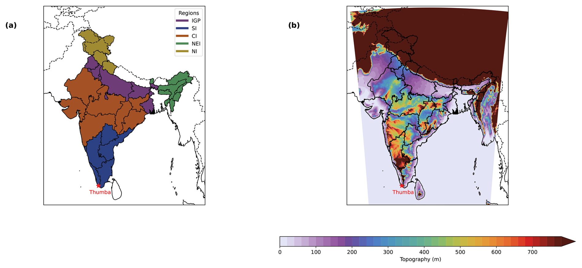
Figure 1 (a) Outlines showing each geographical region of the Indian landmass according to Survey of India (2024) and (b) the topographical height contour of the model domain. CI stands for Central India, NEI for North East India, NI for North India, SI for South India, and IGP for the Indo Gangetic Plain regions.

2.1 TROPOMI observations

The potential of TROPOMI Sentinel-5p to detect significant sources in the single overpass has been demonstrated in recent publications (Hu et al., 2018; de Gouw et al., 2020; Schneising et al., 2020; Chen et al., 2022; Jacob et al., 2022). We utilized TROPOMI CH₄ observations obtained through the Short Wave Infrared (SWIR) band, centered at approximately 2.3 µm. The atmospheric column-averaged CH₄ mixing ratio (XCH₄) is retrieved using the Weighting Function Modified Differential Optical Absorption Spectroscopy (WFM-DOAS) algorithm. The WFMD algorithm uses a least-squares approach based on scaling prior atmospheric vertical profiles to retrieve XCH₄ and XCO simultaneously (Buchwitz et al., 2007; Schneising et al., 2011). Here, we use the WFMD v1.8 algorithm, for which the efficiency has been validated using Total Carbon Column Observing Network (TCCON) measurements, resulting in an improved random error (12.4 ppb) compared to the previous versions (v1.5 and v1.2) (Schneising et al., 2023). For the analysis, we filtered flagged data and utilized only good-quality retrievals represented by xch4_quality_flag = 0.

2.2 Modeling system for atmospheric XCH₄ mixing ratio simulations

We have used the Weather Research and Forecasting model coupled with the Chemistry and Greenhouse Gas module (hereafter referred to as WRF-GHG) for atmospheric CH₄ transport simulations. The core component is the WRF model, based on fully compressible, non-hydrostatic Eulerian equations on terrain-following vertical grids for simulating atmospheric transport (Skamarock et al., 2008). The GHG-TRACER package allows the online passive tracer transport of CH₄ mixing ratio in the atmosphere (Beck et al., 2011; Pillai et al., 2016). The input fluxes from each emission sector are separately provided as “tagged” tracers when added to the first layer in the modeling system. This allows the decoupling of emission contributions to the total atmospheric CH₄ mixing ratio. We have used the WRF-GHG 3.9.1.1 version with a horizontal resolution of 10 × 10 km² (Lambert conformal conic projection grid) and an output temporal resolution of 1 h. The model covers the Indian domain with 307 × 407 grid points and 39 vertical levels. The fifth generation ECMWF reanalysis (ERA-5) data with a horizontal resolution of 0.25° × 0.25° and temporal resolution of 6 h with 137 vertical levels are used as initial and boundary conditions for meteorology (Hersbach et al., 2020; see Table 1). The model is re-initialized each day with

We used the Emission Database for Global Atmospheric Research (EDGAR v7.0; Crippa et al., 2024), Global Fire Assimilation System (GFAS v1.2; Kaiser et al., 2012), and a global wetland CH₄ emissions and uncertainty dataset for atmospheric chemical transport models (WetCHARTs 1.3.1; Bloom et al., 2021) as prior emission fluxes to represent anthropogenic, biomass burning and wetland emissions respectively. We applied temporal scaling factors to the annual EDGAR emissions using step-function time profiles and converted them to 1 h temporal resolution, following Kretschmer et al. (2014). ERA5 meteorology, in which a 6 h spin-up time was configured. For CH₄ mixing ratio fields, initial and boundary conditions are prescribed from the Copernicus Atmosphere Monitoring Service (CAMS re-analysis data). Meteorological fields are reinitialized daily using ERA5 reanalysis, followed by a 6 h spin-up period. In contrast, note that CH₄ tracer fields are initialized only at the beginning of the simulation and the simulated background fields are continuously transported across successive simulation days (i.e. not reintialized daily). This approach ensures that methane concentrations reflect the cumulative influence of emissions, preserving the temporal memory for inverse optimization of local surface fluxes. CAMS provides the simulated atmospheric mixing ratios of CH₄, with a spatial resolution of 0.25° × 0.25° and a temporal resolution of 6 h on 60 vertical levels (Inness et al., 2019; see Table 1). The model utilizes these initial fields to represent the background of the total mixing ratios. Similar to emission flux contributions, we disentangled the background contribution in the model output to investigate its impacts separately. We have also considered the reported level of uncertainties in CAMS-simulated mixing ratios (e.g. Agustí-Panareda et al., 2023; Wang et al., 2023) and applied a monthly scaling factor correction to our methane background (initialized by CAMS) to minimize the unrealistic representation of background contribution to methane mixing ratios. The scaling factor is applied uniformly across the domain to the CH₄ background, specific for each month (i.e., one scaling factor per month). These monthly background scaling factors range from 1 % to 3 %. The corrected WRF-GHG background mixing ratios are hereafter termed simply as background mixing ratios. GFAS data with 0.1° × 0.1° resolution represents biomass burning emissions in the model. GFAS emissions are calculated using fire radiative power observations from the Moderate Resolution Imaging Spectroradiometer (MODIS) instrument aboard the Terra satellite.

WetCHARTs is an ensemble dataset that provides gridded emissions data from 2001 to 2019 at a resolution of 0.50° × 0.50° (Bloom et al., 2017), which were then re-gridded to 0.1° × 0.1° with a temporal resolution of 1 h. The simulated total atmospheric CH₄ mixing ratio thus contains contributions from the initial fields as well as anthropogenic, biomass burning, and biogenic fields of CH₄. Table 1 summarizes the WRF-GHG model set-up used in this study. The general meteorological configuration for the WRF-GHG model set-up applied here is described in Thilakan et al. (2022).

Crippa et al. (2024)Kaiser et al. (2012)Bloom et al. (2017)Hersbach et al. (2020)Agustí-Panareda et al. (2023)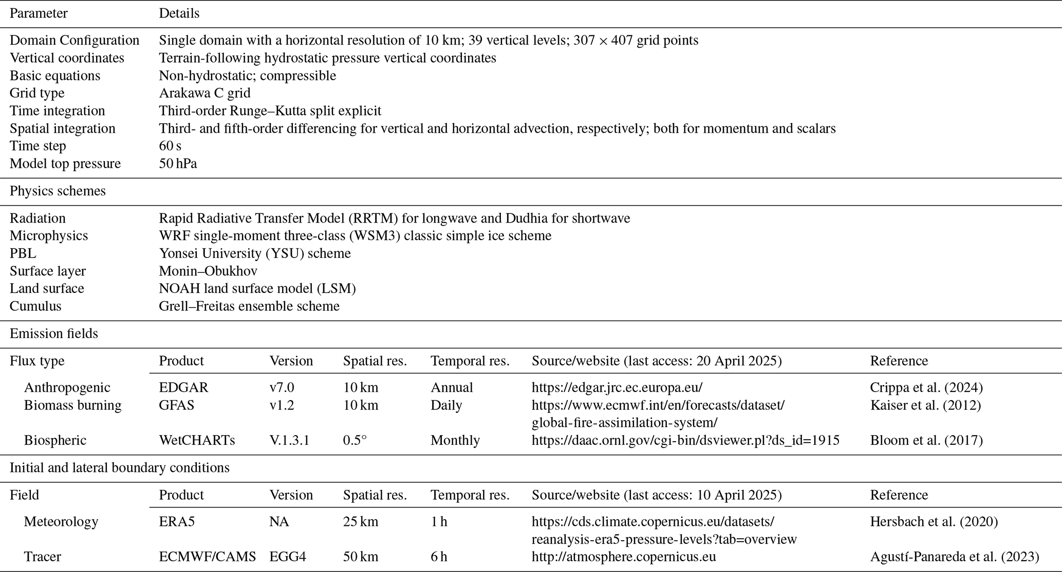

Table 1 WRF-GHG model configuration.

2.3 Ground-level observations

To assess the model's performance at the surface level, a comparative analysis was conducted using CH₄ in situ measurements from a ground-level pollution monitoring station in Thumba (8.5° N, 76.9° E) as denoted in Fig. 1 for 2018 & 2019. Located in southwestern India, Thumba is a tropical coastal station approximately 10 km northwest of Thiruvananthapuram and 500 m inland from the Arabian Sea. This site reflects local to regional influences, but cannot capture the full spatial variability across India. CH₄ concentrations were measured using a greenhouse gas analyzer (model: 911-0011-1001) by Los Gatos Research, USA, based on the off-axis integrated cavity output spectroscopy (OA-ICOS) method (Baer et al., 2002; Raju et al., 2022; Sijikumar et al., 2023; Uma et al., 2024). Air samples were collected from about 10 m above ground level (a.g.l.) using the analyzer's internal pump. Calibration was performed periodically. However, it should be noted that the instrument can be sensitive to temperature, requiring frequent calibration, which was not regularly met. Measurements were recorded at 1 s intervals, with hourly averages used for subsequent analysis. CH₄ measurement uncertainty is 0.25 % (i.e. 5 ppb with respect to 2000 ppb of CH₄) and the reported precision (1σ) is 1 ppb.

2.4 Data post-processing and inverse analysis

We regridded the daily total dry column mixing ratio of CH₄ from TROPOMI at 10 km × 10 km resolution, covering the period from 2018 to 2019. From the hourly WRF-GHG CH₄ mixing ratio simulations generated, we sampled those corresponding to the TROPOMI overpass time for the model domain. The model top is set near ∼50 hPa. When computing the column-averaged mole fractions from simulations, the model profile is extended above the model top utilizing satellite a priori profiles, ensuring the same sampled air column corresponding to the observation datasets, also following a priori profile weights when computing the column-averaged mole fraction (more details below). Here, we assume negligible model biases for the remaining atmospheric contribution above the model top compared to that of the tropospheric and lower stratospheric counterparts. Previous studies of stratospheric and tropospheric contributions to total column CH₄ demonstrated that the model biases in the stratospheric partial column tend to be smaller than those in the tropospheric partial column owing to the substantially higher tropospheric CH₄ contribution to the total column than stratospheric CH₄ (Wang et al., 2017). However, the assumption underlying the extension above the actual model top is a simplification of real-case conditions and may be considered when analyzing the results.

In the present study, the model simulations have not accounted for any impacts of stratospheric CH₄ chemistry reactions on mixing ratios. Ignoring chemical reactions is typically a valid assumption when considering the regional model domain and the considerably longer atmospheric lifetimes of target species, approximately 10 years for CH₄, than the simulation period. Excluding the OH reactions has shown a negligible impact on annual CH₄ at the regional scale, resulting in smaller biases than the measurement uncertainties (1 ppb for in situ measurements and 6 ppb for TCCON) and the typical magnitudes of the observational bias in the inversion (Callewaert et al., 2025). However, atmospheric CH₄ is susceptible to chemical reactions in the stratosphere, which warrants consideration in modelling and analyzing long time series such as decadal contributions.

To ensure a fair comparison with observations, we applied the satellite's averaging kernel (AK), as shown in Eq. (1), accounting for the satellite instrument's vertical sensitivity (Schneising et al., 2019). AK is proportional to the sensitivity profile of the measurement that is weighted with the assumed tracer profiles and provides the relation between the retrieved and known tracer profiles, i.e., applying satellite AK to the model simulations at different vertical levels minimizes the mismatches owing to the instrument vertical sensitivities to the column observations (Eskes and Boersma, 2003; Wang et al., 2023; Schneising, 2024).

We applied the AK to the modeled dry-air CH₄ profiles and derived the dry-air column-averaged mixing ratio of CH₄, Υ_mod, as follows:

$$\begin{array}{}\text{(1)}& {\mathrm{{\rm Y}}}_{\text{mod}}=\sum _l\left({\mathrm{{\rm Y}}}_{\text{apr}}^l+A_l({\mathrm{{\rm Y}}}_{\text{mod}}^l-{\mathrm{{\rm Y}}}_{\text{apr}}^l)\right)w_l\end{array}$$

where l is the index of the vertical layer, A_l is the averaging kernel and ${\mathrm{{\rm Y}}}_{\text{apr}}^l$ is the a priori mole fraction of layer l, and ${\mathrm{{\rm Y}}}_{\text{mod}}^l$ is the corresponding simulated mole fraction of layer l. w_l is the layer-dependent pressure weight.

Hence, Υ_mod (= XCH_4,mod) is used for the model-observation comparisons and inversion analyses. i.e., in this study, Υ_mod represents WRF-GHG XCH₄ simulations.

Estimating optimized CH₄ flux over India

We performed a simple Bayesian inverse optimization to deduce the improved emission estimates over the Indian domain. The inversion is designed in such a way that it describes the relationship between the mixing ratio observations and the surface flux emission information (the unknown state) and a priori information available. This approach allows us to identify the class of possible states consistent with the available information and to assign a probability density function (pdf) to them. The quantities to be optimized, represented by the state vector x with n elements $x_{\mathrm{1}},x_{\mathrm{2}},x_{\mathrm{3}},\mathrm{\dots },x_n$ correspond to the monthly, state-wise emissions from (i) anthropogenic components (EDGAR) and (ii) the sum of anthropogenic (EDGAR) and biomass-burning (GFAS) components, both (i) and (ii) optimized separately. We have omitted the wetland component here since it contributed negligibly to the column-mixing-ratio enhancement. Here, n represents 36 state regions of India. The measured quantities, represented by the measurement vector y with m elements $y_{\mathrm{1}},y_{\mathrm{2}},y_{\mathrm{3}},\mathrm{\dots },y_m$, represent the column observations from TROPOMI over a month at 0.1° × 0.1° spatial resolution. Here, m represents the total number of observations available in each political state.

The relationship between the measurement vector, y, and the state vector, x, can be written as:

$$\begin{array}{}\text{(2)}& \mathit{y}=\mathbf{F}\left(\mathit{x}\right)+\mathit{ϵ}\end{array}$$

where F(x) encapsulates the physics of the measurements as a function of the state vector, described here by our forward model, WRF-GHG, which includes forward transport and mapping of flux fields. The error term ϵ includes model error, representation error (sampling mismatch between the observations and the model), and measurement error.

Linearizing the forward model to a reference state yields:

$$\begin{array}{}\text{(3)}& \mathbf{F}\left(\mathit{x}\right)=\mathbf{K}\mathit{x}+\mathit{ϵ}\end{array}$$

Here, K is the m×n Jacobian matrix, representing the sensitivity of the mixing ratio simulated by the forward model to the state vector. The elements of K are thus: $k_{m,n}=\frac{\partial {\mathbf{F}}_m\left(x\right)}{\partial x_n}$

Since we have not implemented the adjoint model for our forward transport model, the Jacobian matrix is constructed using a finite-difference approach: the transport model (WRF-GHG) is applied to perturbed emissions, and sensitivities of the resulting mixing ratio simulations are derived. This perturbation-based Jacobian construction is mathematically equivalent to computing the response functions to state vectors. The Jacobian matrix in the present study ensures capturing near-field influence on observations and minimizes the over-interpretation of far-field influences. For robust flux estimations at regional and sub-regional scales, it is widely accepted that increasing reliance on near-field sensitivity minimizes the ill-posed solutions (Nesser et al., 2024; Munassar et al., 2023; Ware et al., 2019; Pillai et al., 2012; Gerbig et al., 2006).

The elements in the Jacobian matrix are derived as follows:

$$\begin{array}{}\text{(4)}& k_{m,n}={\displaystyle \frac{({\mathrm{{\rm Y}}}_{\mathrm{pert}}{)}_m-{\mathrm{{\rm Y}}}_m}{({\mathrm{\Phi }}_{\mathrm{pert}}{)}_n-{\mathrm{\Phi }}_n}}\end{array}$$

The above derivation closely follows methods implemented in Pillai et al. (2016), Ye et al. (2020) and Kuhlmann et al. (2020). Here, Υ and Υ_pert are the 1-D representations of the column mixing ratio and the perturbed column mixing ratio, respectively, both derived by our forward model, corresponding to each m elements in the measurement vector y. Φ and Φ_pert represent emissions and perturbed emissions, respectively, corresponding to each n elements in the state vector x. Note that perturbed mixing ratios are simulated by applying the transport operator (WRF-GHG) to perturbed emissions, as explained before. By our design, the elements in the y correspond to the available column mixing ratio observations over a month at 0.1° × 0.1° spatial resolution, and the elements in the x refer to total monthly emissions of each political state.

In our implementation, we focus on anthropogenic fluxes and their contributions to atmospheric dry-air column mixing ratios. x_A represents the prior fluxes, which consist of monthly anthropogenic (major contributions from enteric fermentation, agricultural soil, waste water handling, and fuel exploitation) and biomass burning emissions. The inversion optimizes the corresponding total emissions per state by minimizing the model-observation mismatches. The background contributions are removed from the observations to target optimizing the regional enhancement fluxes. i.e., the measurement vector y consists of column observations from TROPOMI subtracted by simulated background mixing ratios over a month at 0.1° × 0.1° spatial resolution.

The background mixing ratios are simulated by WRF-GHG, as explained in Sect. 2.2. We have considered measurement errors (including forward model errors) and prior errors: S_e and S_a represent measurement error and prior error covariance matrices, respectively. The measurement error covariance matrix S_e consists of retrieval (y) and the forward model (F(x)) errors for methane. We assumed a prior emission uncertainty of 80 % and a measurement uncertainty of 16 ppb, as adopted from Liang et al. (2023), calculated using the residual error method (Heald et al., 2004). We have not considered cross-correlations; hence, only the diagonal elements of the matrices S_e and S_a are non-zero.

Since multiple observational products are available and we may expect differences among those products, we assess product differences across our region using scientific, operational, and GOSAT-blended products. The additional data products are: the operational Sentinel-5P/TROPOMI Level-2 methane product provided by ESA/Copernicus (Copernicus Sentinel-5P, 2021), and the blended TROPOMI + GOSAT methane product available from April 2018 (Balasus et al., 2023). Further, we conduct an additional inversion by inflating the measurement uncertainty by more than 50 % (∼25 ppb) to examine the influence of product differences on posterior flux uncertainties.

The solution to the inverse problem is obtained by minimizing the Bayesian scalar cost function J(x) (Rodgers, 2000):

$$\begin{array}{}\text{(5)}& J\left(\mathit{x}\right)=(\mathit{x}-{\mathit{x}}_{\mathrm{A}}{)}^{\mathrm{T}}{\mathbf{S}}_{\mathrm{a}}^{-\mathrm{1}}(\mathit{x}-{\mathit{x}}_{\mathrm{A}})+(\mathit{y}-\mathbf{K}\mathit{x}{)}^{\mathrm{T}}{\mathbf{S}}_{\mathrm{e}}^{-\mathrm{1}}(\mathit{y}-\mathbf{K}{\mathit{x}}_{\mathrm{A}})\end{array}$$

where ∇_xJ(x)=0, the optimal estimate $\widehat{\mathit{x}}$ is obtained (Rodgers, 2000). The state that maximizes the posterior pdf P(x|y) is the maximum a posteriori solution (MAP). The maximum a posteriori solution is obtained as follows:

$$\begin{array}{}\text{(6)}& \widehat{\mathit{x}}={\mathit{x}}_{\mathrm{A}}+{\left({\mathbf{K}}^{\mathrm{T}}{\mathbf{S}}_{\mathrm{e}}^{-\mathrm{1}}\mathbf{K}+{\mathbf{S}}_{\mathrm{a}}^{-\mathrm{1}}\right)}^{-\mathrm{1}}{\mathbf{K}}^{\mathrm{T}}{\mathbf{S}}_{\mathrm{e}}^{-\mathrm{1}}\left(\mathit{y}-\mathbf{K}{\mathit{x}}_{\mathrm{A}}\right)\end{array}$$

Thus, $\widehat{\mathit{x}}$ represents the optimized spatially averaged monthly anthropogenic and biomass burning fluxes corresponding to each political state considered. The posterior error covariance matrix, denoted by $\widehat{\mathbf{S}}$, is derived as follows.

$$\begin{array}{}\text{(7)}& {\displaystyle }\widehat{\mathbf{S}}=({\mathbf{K}}^{\mathrm{T}}{\mathbf{S}}_{\mathrm{e}}^{-\mathrm{1}}\mathbf{K}+{\mathbf{S}}_{\mathrm{a}}^{-\mathrm{1}}{)}^{-\mathrm{1}}\end{array}$$

The error reduction for each month following the inversion procedure ($\stackrel{\mathrm{̃}}{e}$) is calculated as follows:

$$\begin{array}{}\text{(8)}& \stackrel{\mathrm{̃}}{e}=\mathrm{1}-{\displaystyle \frac{{\mathit{\sigma }}_{\mathrm{post}}}{{\mathit{\sigma }}_{\mathrm{prior}}}}\end{array}$$

where σ_post is derived as the square root of the diagonal elements of $\widehat{\mathbf{S}}$. Similarly, σ_prior is obtained from the square root of the diagonal elements of the prior error covariance matrix.

The national budget for annual optimized fluxes ${\widehat{\mathit{x}}}_{\mathrm{annual}}$ (in Tg yr⁻¹) is derived as:

$$\begin{array}{}\text{(9)}& {\widehat{\mathit{x}}}_{\mathrm{annual}}=\sum _{t=\mathrm{1}}^{N_t}\sum _{s=\mathrm{1}}^{N_s}{\widehat{\mathit{x}}}_{s,t},\end{array}$$

where ${\widehat{\mathit{x}}}_{s,t}$ represents the estimated value at each political state s for the corresponding month t. N_s is the total number of political states, and N_t is the total number of months considered.

3 Results and Discussion

3.1 Regional and sectoral distribution of CH₄ sources

The bottom-up inventories such as EDGAR v8.0 (latest release; Crippa et al., 2024), WetCHARTs v1.3.1, and GFAS v1.2. relate the GHG emissions to the causative processes by considering emission activities and emission factors, thereby providing us with a “first guess” to identify the prominent sources (Miller and Michalak, 2017), although with inherent uncertainties. In this section, we present a detailed comparative assessment of the sectoral and regional distributions of different CH₄ sources (such as enteric fermentation, wastewater handling, rice agricultural land, wetlands, and biomass burning).

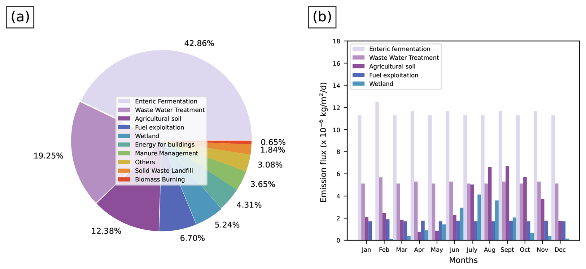
Figure 2 (a) The percentage of contributions of different CH₄ sources towards total annual emission flux over the Indian domain, (b) monthly contribution (calculated from the EDGAR temporal profiles described in Crippa et al., 2020) from each source.

Our sector-wise analysis of the bottom-up inventories shows that the enteric fermentation associated with the digestive process in cattle makes a significant contribution to CH₄ emissions in India (42.9 %), followed by wastewater treatment (19.2 %), agricultural soil (12.4 %), fuel exploitation (6.7 %), and wetland (5.2 %, excluding agriculture) (see Fig. 2). The sources with significant seasonality include agriculture (see Fig. 2b) and biomass burning, also reported in Ganesan et al. (2017). Figure S1a–d in the Supplement shows an annual average of the spatial distribution of CH₄ emissions for the four major emission sectors in 2018. Anthropogenic sources are expected to provide the bulk of India's CH₄ emissions, especially livestock, rice cultivation, and waste management (Maasakkers et al., 2019). The annual CH₄ emissions corresponding to rice cultivation (emission from the sector “Agricultural soil” as given by the EDGAR inventory) show a peak in values over the Indo-Gangetic Plain (IGP) region (Fig. S1c). Several other studies have used GOSAT and other data sources to analyse the CH₄ emissions from rice paddies in India (Miller et al., 2019; Ganesan et al., 2017; Anand et al., 2005). Previous studies reported CH₄ emissions from rice paddies in India of about 3.9 Tg yr⁻¹, with the bulk emitted between June and September (Janssens-Maenhout et al., 2011; Garg et al., 2011; Panigrahy et al., 2010). The sector-wise analysis of the EDGAR inventory for the year 2018 shows significant CH₄ highs on the eastern coast, including West Bengal and Odisha, which can be attributed to the large rice cultivation in these regions (Crippa et al., 2024). The analysis of monthly emissions from rice cultivation over the year 2018 indicates an increasing pattern in summer monsoon seasons, June to September (see “Agricultural soil” in Fig. 2b), with the maximum in August (16.9 %) and September (16.5 %) and the minimum in April (1.9 %); percentages are shares of the annual flux. There is a smaller peak in February–March time, owing to winter rice cultivation, which comprises 14 % of total rice production in India (Manjunath et al., 2006). Similarly, in the wetland emissions, we also see an increase in monsoon months (Fig. 2b). The peak wetland emissions are seen in July (24.6 %), followed by August (21.4 %), and the minimum in January (0.2 %). It has been previously reported from satellite observations that the waterlogged areas increase nearly threefold from the beginning to the end of the monsoon, resulting in higher wetland CH₄ emissions (Agarwal and Garg, 2009). The pre-monsoon CH₄ emission (15.5 %) is higher than post-monsoon (6.2 %; see Fig. 2b, possibly due to higher temperatures during the pre-monsoon season as described in Das et al. (2023). Our analysis of monthly emissions based on GFAS shows a peak due to biomass burning in March (65.4 %), with the lowest burning reported in July (0.1 %) (Fig. 3e–h). Other sources of CH₄, including fossil-fuel emissions, enteric fermentation, and wastewater handling, have not shown considerable seasonal variability. A similar pattern has also been observed from the 2019 anthropogenic and natural CH₄ emission analysis (figure not shown).

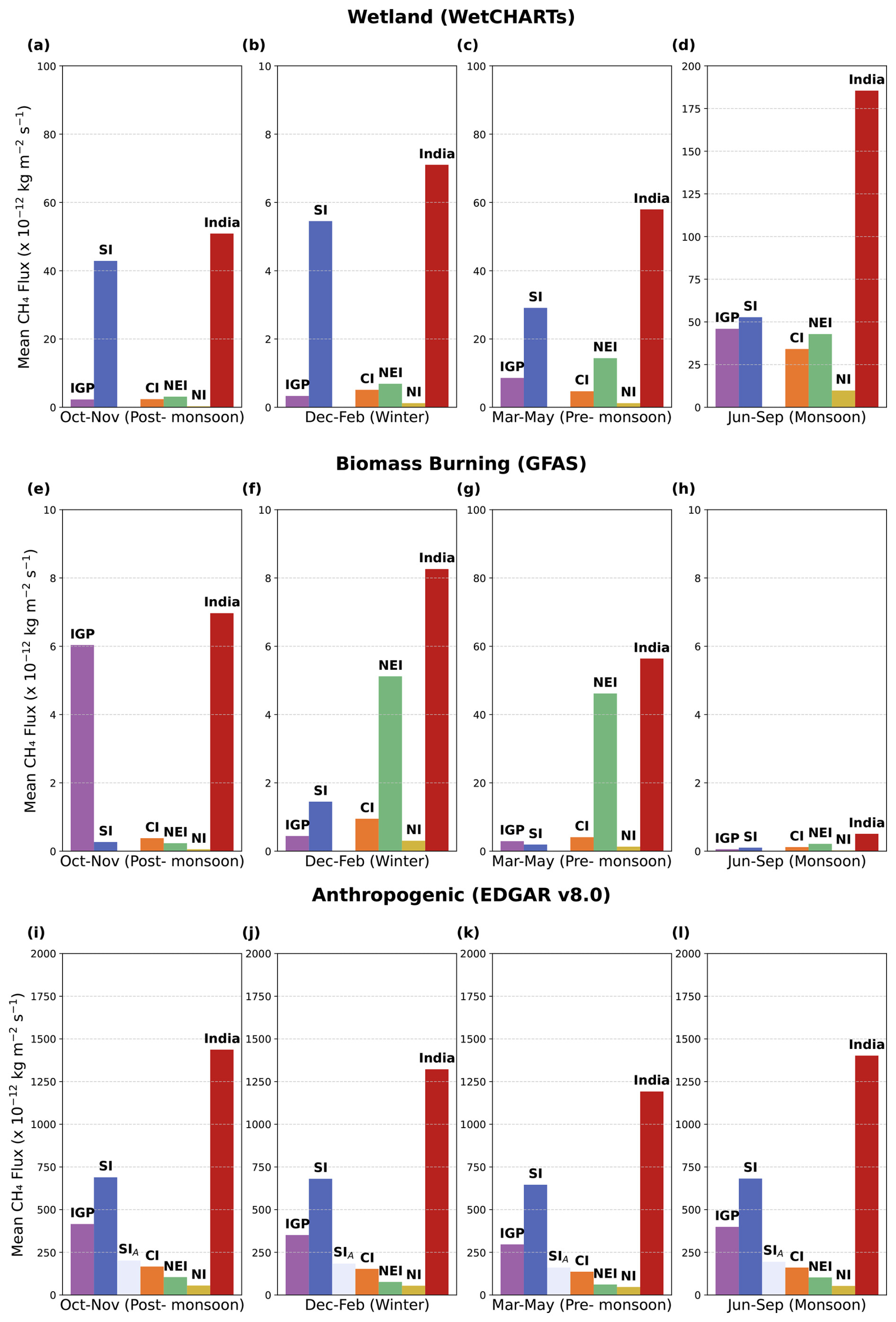
Figure 3 Seasonal mean emissions from (top panels) wetland, (middle panels) biomass burning, and (bottom panels) anthropogenic sources, separated for seasons, for each region as specified in Fig. 1. Note: The ranges of the y-axes are not uniform in panels to improve visibility.

Further, the anthropogenic emissions remain the largest contributors to regional CH₄ emissions (see Figs. 3 & S2). The total anthropogenic emissions, reported by the EDGAR bottom-up inventory (version 8), peak seasonally in the South India (SI) region (>700 × 10⁻¹² kg m⁻² s⁻¹), followed by IGP (>400 × 10⁻¹² kg m⁻² s⁻¹), with the minimum emissions observed in North India (NI; see Fig. 3). The peak is typically in October–November, followed by June–September, with a minimum in March–May. Total anthropogenic emissions over India show a peak in October–November and a dip in March–May (1410–1090 × 10⁻¹² kg m⁻²). While IGP shows high magnitude in spatial distribution (see Fig. S1a–d), SI contributes more emissions due to emission hotspots. Four hotspots identified (see Fig. S3) in SI include one city – Namakkal (11.25° N, 78.15° E; HS1) and three villages – Mandapaka Rural (16.75° N, 81.65° E; HS2), Pasumamla (17.35° N, 78.65° E; HS3), and Mulkalappalli (18.65° N, 79.55° E; HS4). Excluding these hotspots (SI_A) shifts the highest emissions to IGP (see Fig. 3i–l). Namakkal in Tamil Nadu faces poultry waste deposition, potentially increasing methane emissions (Ramasamy and Manivel, 2019). Mandapaka in Andhra Pradesh, known as the “rice bowl” of the region, contributes to higher agricultural rice emissions (Gururaj Katti et al., 2002). Pasumamla in Telangana sees significant poultry waste dumping in landfills (https://rangareddy.telangana.gov.in/animal-husbandry, last access: 12 February 2025). Mulkappalli, a coal mining site in Telangana, contributes to the high CH₄ levels in the inventory (https://khammam.telangana.gov.in/economy, last access: 12 February 2025). Figure S4 shows the methane hotspots over the Indian domain from the coal mining sector as derived from the EDGAR inventory.

Based on WetCHARTs (version 1.3.1), natural wetland emissions are approximated at 1.7 Tg yr⁻¹, with peak emissions occurring from June to September (∼ 185 × 10⁻¹² kg m⁻²). The highest wetland emissions (>25 × 10⁻¹² kg m⁻² s⁻¹) are seen over the SI region in June–September, October–November, and March–May, with a peak of ∼ 50 × 10⁻¹² kg m⁻² s⁻¹ (Fig. 3). These peaks are likely due to increased waterlogged areas during the monsoon (Fig. 2b). Biomass burning emissions, smaller than wetland and anthropogenic emissions, peak in March–May in most regions except the IGP, where crop residue burning occurs from October to November (Deshpande et al., 2022, 2023). The North East India (NEI) region shows the highest biomass burning emissions in March–May (∼47 × 10⁻¹² kg m⁻²), likely due to slash-and-burn practices before planting (Deshpande et al., 2023. Total emissions, combining anthropogenic (EDGAR), wetland (WetCHARTs), and biomass burning (GFAS) emissions, peak in October–November and June–September, with the SI region contributing the highest share (49.2 % and 46.4 %, respectively), and 52 % in March–May and 51.7 % in December–February (Fig. S5).

Though the above estimations give an overview of Indian CH₄ source contributions and their regional patterns, there have been increased concerns about their accuracy due to methodological weaknesses and data gaps (Solazzo et al., 2021; Madrazo et al., 2018). For example, the combined emissions from Oil, Gas, and Coal over the Indian region reported by Scarpelli et al. (2025) is 1.8 Tg yr⁻¹, whereas EDGAR reported 2.2 Tg yr⁻¹. Also, bottom-up methods can overestimate or misinterpret emission sources even at the global level (Saunois et al., 2016). Though inverse modeling can improve the CH₄ budget significantly, its potential to minimize biases in the bottom-up models used as prior estimates may be limited by insufficient coverage of mixing ratio observations and its inadequate representation in the forward models. Satellite instruments such as TROPOMI may aid in high observation density with good spatial coverage (Palmer et al., 2021), the potential of which in the Indian context is explored in further sections.

3.2 Assessment of the forward-model performance against surface measurements

As discussed in Sect. 2.3, we utilized hourly ground-based observations from a ground-based site, Thumba, to assess the WRF-GHG performance in the planetary boundary layer. The lowest level (approximately 35.2 m) of WRF-GHG-simulated CH₄ at Thumba is compared with surface-level observations of CH₄ and is presented here. Generally, the analysis indicated a reasonable performance of WRF-GHG simulations. CH₄ mixing ratios are found to be lowest during the monsoon season (June–August), increasing from early October and peaking during the post-monsoon and winter months (November–January; see Fig. 4a). The maximum values are seen in December (∼ 2100 ppb). The hourly observations show high variability (about 112.7 ppb), but ranging from 1817.4 to 2612.6 ppb for 2018–2019; see Fig. S6. Despite some discrepancies, the WRF-GHG simulations broadly align with those highly fluctuating observation patterns, capturing about 56 % of the observed variability. In October, monthly averaged WRF-GHG simulations and TROPOMI observations are strongly correlated, although their absolute values differ substantially (Figure not shown). The mean difference between observations and simulations is 47 ppb, but it shows large model-observation variability of up to 73.9 ppb (Figs. 4a and S6a). However, this large discrepancy between the model and observations can be attributed to the influence of fine-scale nocturnal coastal meteorological conditions at the measurement site, as reported in Kavitha et al. (2018). Considering only the afternoon hours, the model-observation differences are reduced to 6.4 ppb, with a maximum difference varying up to 28.1 ppb, capturing about 79 % of observed variability (Figs. 4b and S6b). The comparison has also been performed by removing the boundary contributions from CAMS (see Fig. S7), showing that enhancements correlate with observed variability (R²=0.48). Thus, the above comparison suggests the potential of our model in representing the regional and seasonal variations. The above result is promising, confirming the usability of those afternoon measurements representing well-mixed atmospheric conditions, which can be utilized for future carbon assimilation systems in conjunction with a high-resolution forward modeling framework. As seen for all hours, WRF-GHG generally underestimates surface CH₄ mixing ratios (Fig. S6). Notably, the model-observation differences peaked in winter, owing to the unusually high variability seen in the observations during this period. The effect of enhanced vertical mixing can be seen in the summer months, causing low observed CH₄ magnitude and associated mixing ratio variability. Noteworthy is that the magnitude of observed CH₄ is found to be the smallest during the summer monsoon. While the shallow planetary boundary layer (PBL) in the winter accumulates the effect of surface emissions to the lower boundary, increased boundary layer mixing in the summer can cause lower CH₄ magnitude and variability. Further, Guha et al. (2018) and Metya et al. (2021) report that the influx of clean air from the Southern Hemisphere, carried by the monsoonal south-westerly winds, can influence the surface CH₄ to lower its concentration. The high rates of OH radical oxidation may also influence surface CH₄ mixing ratios (Lin et al., 2015).

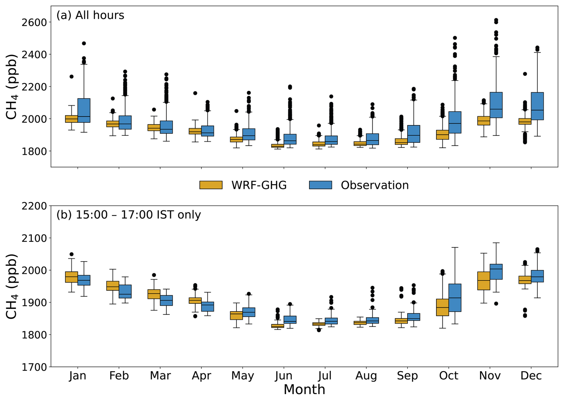
Figure 4 Monthly distribution of observed and WRF-GHG simulated CH₄ mixing ratios at Thumba for 2018 & 2019 for (a) all hours and (b) only 15:00–17:00 Local Time (IST hours) (25th and 75th quartiles; see the site location as denoted in Fig. 1). Note that the ranges of the y-axes are not uniform in panels to improve visibility.

Even though WRF-GHG has shown reasonable performance in evaluating ground-based observations from a complex site (located near the southernmost coastal boundary of the model domain), the model's robustness needs to be further examined across multiple locations in India when available. Those evaluations are particularly necessary for assessing our confidence in the derived posterior fluxes. Although we found that local fluxes had a more dominant contribution to the observed variability than the background contributions (see Fig. S7), there can be non-negligible differences arising from the choice of global model products used for initialization. For instance, we conducted additional analysis comparing the CAMS EGG4 product, which was used for initialization in this study, with the inversion-optimized CAMS product (Bergamaschi et al., 2013). This comparison indicated a difference of approximately 13 ppb over India (see Fig. S8). While it is expected that only a small fraction (less than 10 % to 15 %) of these initial tracer differences will effectively converge to influence model simulations (e.g. Monteil et al., 2011), the potential impact of various tracer initializations on model simulations over this region is not addressed in the current study. The above aspect is worth a future investigation through a dedicated model sensitivity study.

3.3 Anthropogenic XCH₄ mixing ratio enhancements

In this section, we discuss the mixing ratio enhancements in the atmospheric column in response to spatial and temporal distributions of regional sources for the period 2018–2019. i.e. by considering only contributions from the sum of anthropogenic and biomass-burning emission sources (mostly human-influenced in India, i.e, from agricultural residue burning and managed fires) over the model domain and not using CAMS-derived background XCH₄ (see Sect. 2.2). As mentioned in Sect. “Estimating optimized CH₄ flux over India”, we have also omitted the wetland (biogenic) component here since it contributed negligibly to the column-mixing-ratio enhancement (see Figs. S9 & S10). The IGP region exhibits significant XCH₄ enhancements (from 27 to 67 ppb) from regional sources attributed to anthropogenic and biomass-burning fluxes (see Fig. 5). Seasonally, the highest XCH₄ enhancements occur during winter (with a maximum of ∼ 251 ppb in January; see Fig. S11) over India. The minimum enhancement for the whole Indian domain occurs during the monsoon season (June–September), likely due to a combination of higher boundary layer heights and stronger winds, which enhance vertical and horizontal transport affecting column CH₄ concentrations. The concentrations may also be impacted by the seasonal changes in regional or larger fluxes (>1000 km); however, further investigation is needed to assess their contributions.

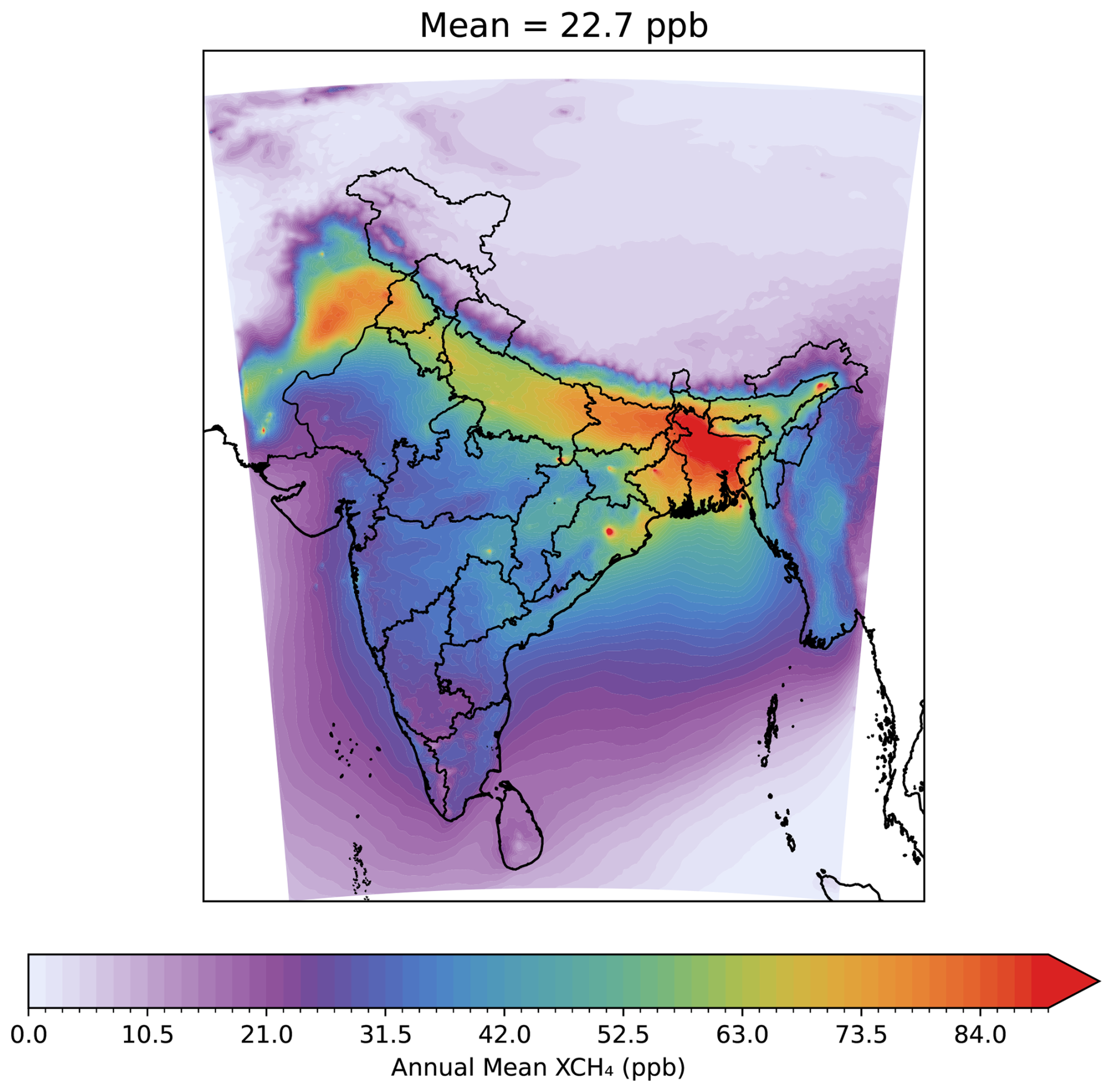
Figure 5 Spatial distribution for annual WRF-GHG simulated anthropogenic mixing ratio enhancement of XCH₄ (including biomass burning) for 2018.

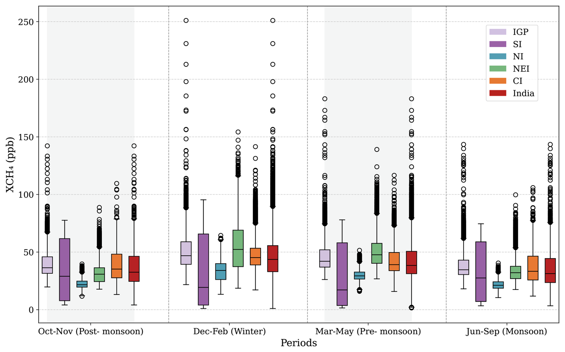
Figure 6 Distribution of seasonal average of simulated mixing ratio enhancement (XCH_4,ant + XCH_4,bbu) over different regions of India in 2018. The box plot displays medians, interquartile ranges, and minimum and maximum values, with data points beyond 1.5 times the interquartile range represented as outliers.

Figure 6 shows the regional variability of anthropogenic XCH₄ enhancements across different parts of India as shown in Fig. 1. The highest regional magnitudes and variability in mixing ratio enhancements occur in the winter season. Here, consistently high magnitude in spatial distribution is found over the IGP region (with a median of ∼50 ppb), showing maximum values over the SI region (∼90 ppb) owing to emission hotspots. During winter, the NEI shows high XCH₄ enhancements, with values reaching up to 115 ppb (with a median value of ∼60 ppb). Winter peaks in XCH₄ likely arise from stable atmospheric transport that carries and concentrates emissions from the preceding October–November period. From June to September, SI enhancements reach up to ∼75 ppb (with a median value of ∼25 ppb). A similar trend is seen for 2019 (Figure not shown). SI exhibits the widest interquartile range with the lowest minimum value, a relatively low median, and the highest maximum in most seasons, indicating the influence of hotspot emissions, as discussed earlier in Sect. 4.1.

3.4 Comparison of modeled and observed total XCH₄

In this section, we present our comparisons of WRF-GHG simulations with TROPOMI observations of total XCH₄ in 2018, considering all months in which reasonable amounts of satellite measurements are available after filtering. The details of filtering are provided in Schneising et al. (2023). TROPOMI observations show distinct seasonal variations in the large spatial domain (Fig. 7), possibly resulting from both atmospheric transport and surface emissions variations. Observations indicate highest values in the mean spatial distribution of XCH₄ from October to November within the range of ∼ 1862 to 1870 ppb. These seasonal increments can be attributed to the combination of surface emissions, boundary layer height, and horizontal transport, which accumulates the effect of the distribution of tracers at lower atmospheric levels. These increased regional emissions, especially from anthropogenic sources, are also seen in Figs. S2 & 3, which are typical for some parts of India, like the SI and IGP, during the October–November season. However, we cannot neglect the likelihood of bias in the observations due to high aerosol loads, which impacts XCH₄ retrievals (Lorente et al., 2021; Hu et al., 2018; Pandey et al., 2019). All the months show significantly higher total XCH₄ mixing ratios over the IGP region in comparison with the other regions over India. The IGP region is more prone to biomass burning in October and November, causing more aerosols in the region. We have examined the particulate matter (PM_2.5) content using the MERRA database, which indicates a heavier aerosol content due to burning during the winter, not always necessarily peaking in October but during the December–February season (Figure not shown). There is a gradual increase in XCH₄ mixing ratios beginning from the winter month of January till March, with a slight dip in April and then a distinctly high increment in October (exceeding 1870 ppb) in October over the IGP (see Fig. 7a–f).

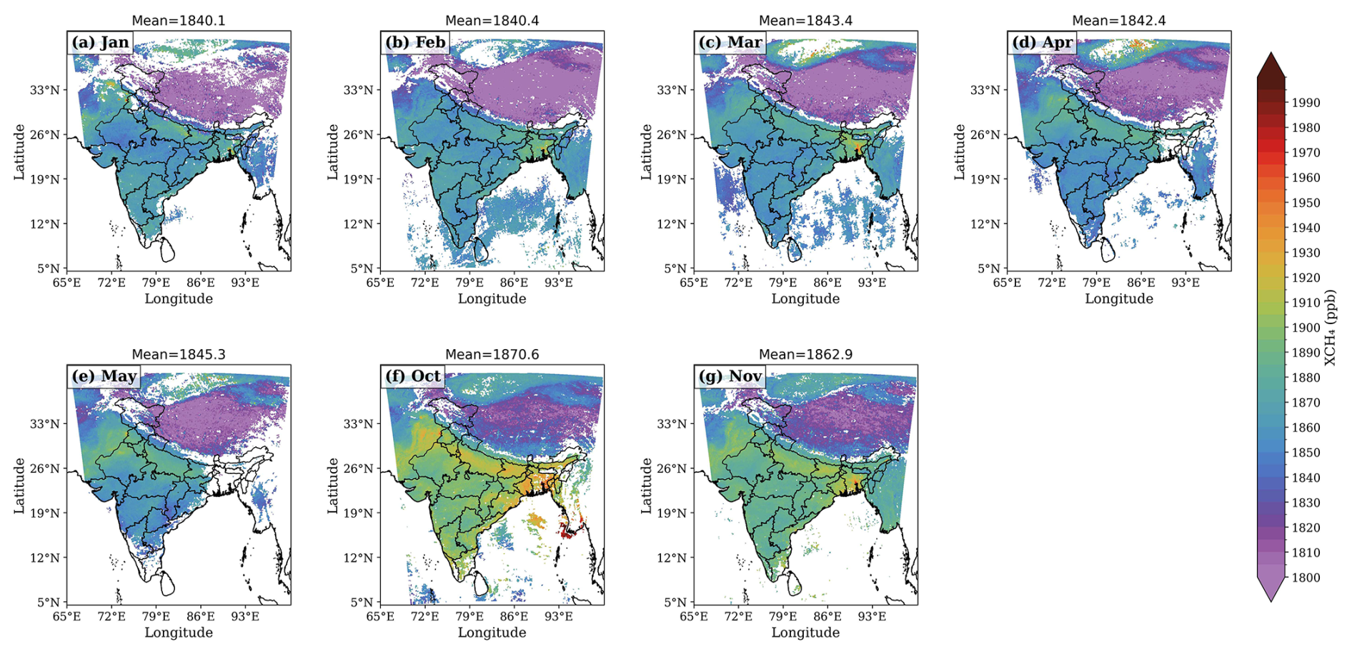
Figure 7 Spatial distribution of the TROPOMI Sentinel-5P measurements, averaged for (a)–(g) each available month in 2018. Some months are excluded due to insufficient data points, due to filtering using the quality flag as given in the data product.

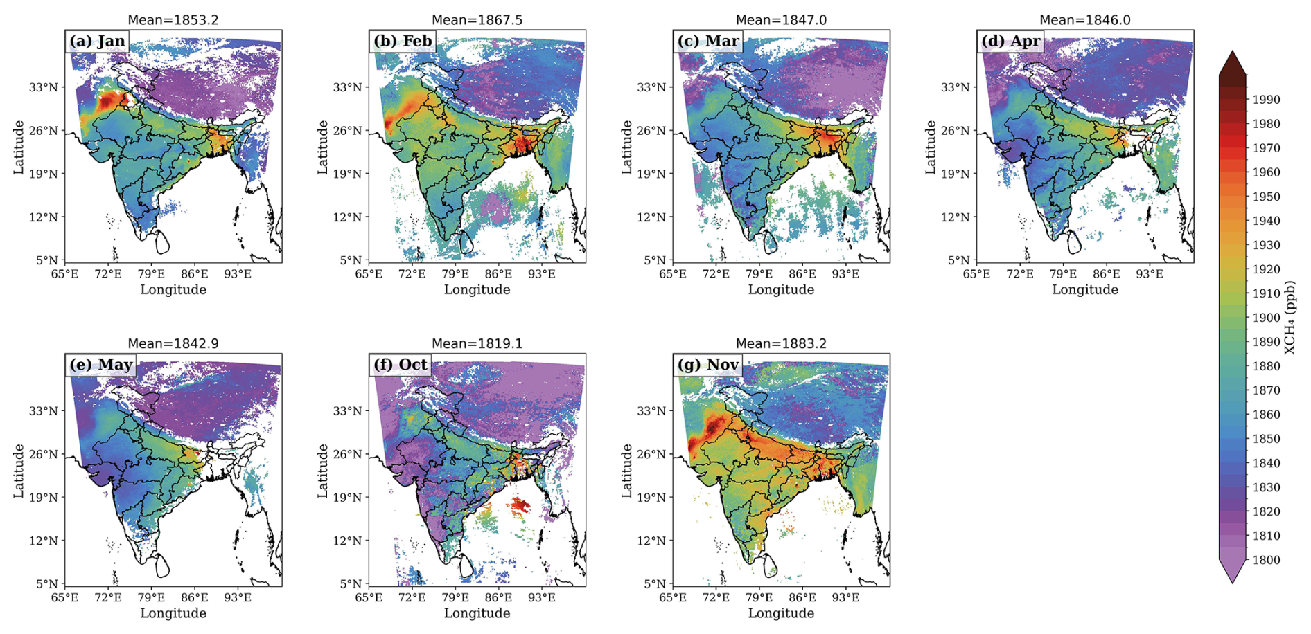
Figure 8 Same as Fig. 7, but showing WRF-GHG simulations of total XCH₄.

We find that the WRF simulations generally overestimate the total XCH₄ mixing ratio over the Indian region compared to TROPOMI observations, peaking in winter months (maximum at 1883 ppb; see Fig. 8). The IGP emission hotspot is also pronounced in the EDGAR inventory (Fig. S1, see Sect. 4.1), suggesting the large impact of anthropogenic emissions on the observed total XCH₄. Further, the sectoral analysis of the EDGAR emission inventory and the consistency of the spatial pattern with TROPOMI observations indicate that the enhancement over the IGP hotspot can be attributed to anthropogenic emissions from the large cattle population and agricultural activities, especially rice production. Similarly, high XCH₄ values observed along the eastern coast during October and November can be attributed to the agricultural soil emissions, as seen in Fig. S1c. Wetland emissions also peak on the eastern coast, but the emissions are not found to be high enough to affect the mixing ratio enhancement significantly (see Figs. S9 & S12). Table S1 in the Supplement shows the mean observed XCH₄ and the variability over the entire study domain for the non-monsoon months of 2018 and 2019.

In general, the WRF-GHG simulations tend to show high bias in the winter months (see Fig. 9). A definite and widespread underestimation by the model was found in October 2018. However, in 2019, WRF-GHG was almost able to capture the observed XCH₄. In the summer months, the model shows patterns of overestimation in eastern India and underestimation in western India. These regional differences in patterns of XCH₄ can arise from heterogeneous sectorial distributions of surface emissions with seasonality that would have been misrepresented in the inventories in conjunction with the large-scale meteorological influences (e.g. southwest monsoon over India, Chandra et al., 2017).

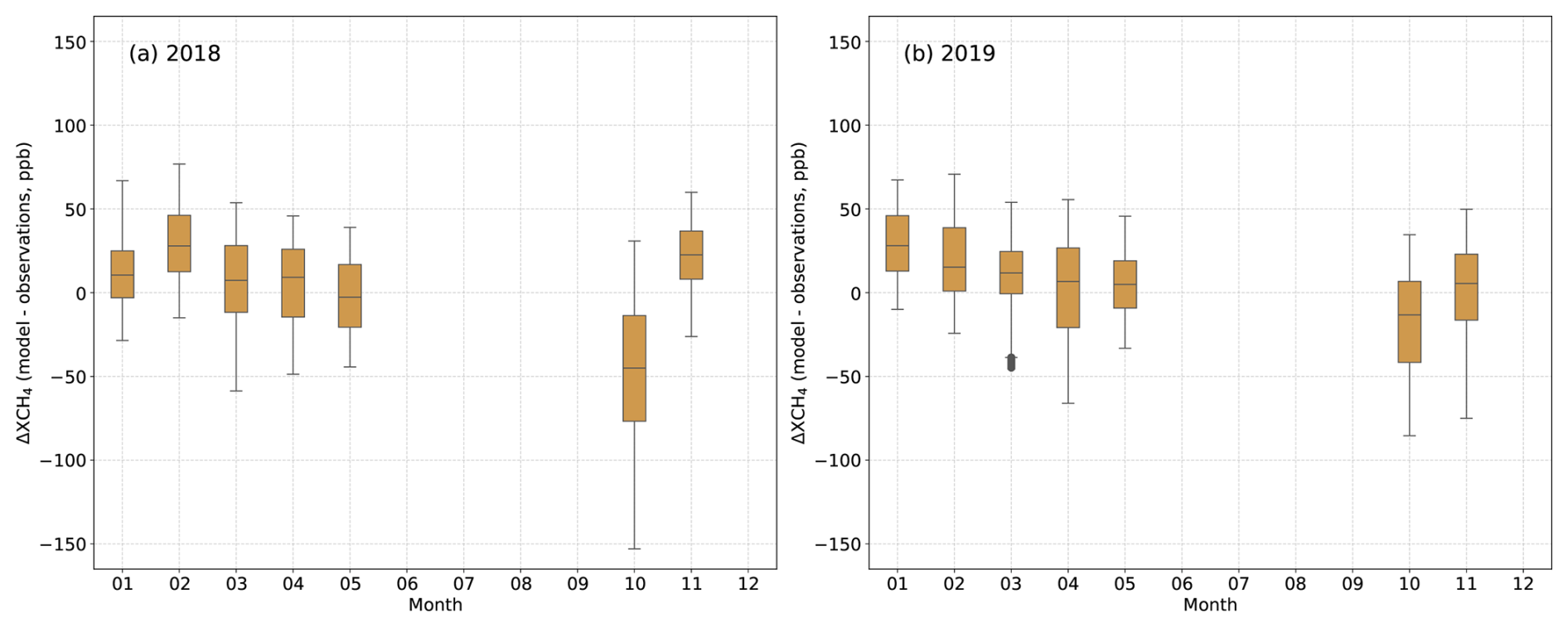
Figure 9 Monthly distribution of the difference between WRF-GHG simulations and TROPOMI Sentinel-5p retrievals of XCH₄ for each available month in 2018 and 2019 when sufficient observations are available (Outliers are not removed; instead, a 90 % winsorization (Wilcox, 2005) is applied for the outliers.)

While the peak total column XCH₄ for TROPOMI falls in October (∼ 1870 ppb), that of the WRF-GHG simulations is in November (∼ 1883 ppb). However, it is noteworthy that both the model and observation indicate the XCH₄ peak in either of the winter months between October and February. The WRF-GHG simulations show a higher variability (standard deviation) than observations for each month. WRF-GHG overestimates the XCH₄ values with a bias of ∼ 13 (29) ppb in 2018 (2019) (see Table S1).

3.5 National CH₄ budget estimation via inverse optimization

In this section, we present estimates of India's anthropogenic CH₄ budget for the period 2018–2019 derived through inverse optimization as described in Sect. 3.2. Two separate inversions were performed using identical model configurations and observational constraints: one including biomass-burning emissions from GFAS in addition to anthropogenic sources, and another excluding biomass-burning emissions. Posterior emission estimates from both inversions are reported separately to quantify the impact of biomass burning on inferred anthropogenic CH₄ emissions.

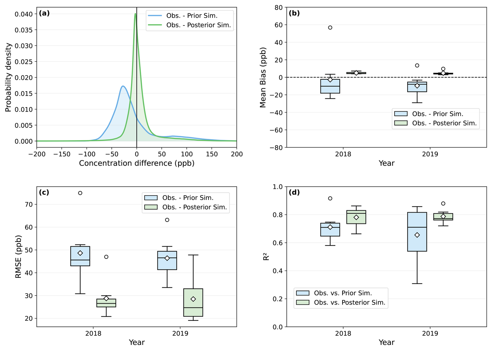
Figure 10 Model-Observation mismatches before and after optimization: (a) Probability density for difference between observed (Obs.) and simulated (Sim.) concentrations, (b) monthly Mean Bias, (c) monthly RMSE and (d) R² between observations and simulations before (blue) and after (green) optimization. In the legend, the terms Prior Sim. and Post Sim refer to simulations before and after optimization, respectively.

The model-observation mismatches before and after optimization are shown in Fig. 10. The optimization significantly reduces mismatches in XCH₄ as expected for a robust inversion, resulting in a narrower distribution around zero. For example, in January 2018, the mean XCH₄ bias improves from −12.4 ppb (before optimization) to 5.2 ppb (after optimization). Simultaneously, the improved explanation of variance in statistics is found, indicating a better fit to the observed data after optimization (see Fig. 10).

The EDGAR emission inventory reports an annual mean CH₄ emission budget of 28.8 Tg yr⁻¹, and we assumed 80 % uncertainty (23 Tg yr⁻¹) in our prior as discussed in Sect. 3.1. The posterior annual emission estimate is 23.4 Tg, with the uncertainty reduced to 3.3 Tg. The percentage of error reduction (calculated using Eq. 8) for monthly posterior fluxes ranges from 68 % to 92 %. Our inverse model results indicate an overestimation of 13 % to 24 % in the EDGAR inventory. Incorporating biomass burning emissions from GFAS has an impact of +0.3 Tg yr⁻¹ on both prior and posterior emission estimates over the Indian region.

As per the India Fourth Biennial Update Report (BUR4) submitted to the United Nations Framework Convention on Climate Change (UNFCCC) (MoEFCC, 2024), the CH₄ emission budget for India is approximately 19.6 Tg yr⁻¹, which is around 32 % less than the EDGAR-reported emissions during the 2018–2019 period. Previous studies also reported an overestimation of the global emission inventories over India. For instance, Qu et al. (2021) reports 41–57 Tg yr⁻¹ anthropogenic CH₄ emission from India, which is significantly higher than our estimations. Also, Zhang et al. (2021) estimates Indian anthropogenic methane emissions of 33±0.6 Tg yr⁻¹, higher than this study estimates. However, the Global Methane Budget (2000–2017, Saunois et al., 2020), based on top-down approaches using in-situ and GOSAT observations, suggests 25 Tg yr⁻¹ of anthropogenic CH₄ emissions from India, but acknowledges large uncertainty ranges in their estimates. Also, bottom-up models' estimates that are compiled in Saunois et al. (2020) and Jackson et al. (2020) indicate a mean anthropogenic CH₄ emission of 21–24 Tg yr⁻¹ from India. The above two estimates align with our results, though we used independent observations and a different modeling approach. The recent updates on the Global Methane Budget (2000–2020, Saunois et al., 2025) indicate anthropogenic methane emissions of 37–49 Tg yr⁻¹ for South Asia (including Afghanistan, Bangladesh, Bhutan, India, Nepal, Pakistan, and Sri Lanka), in which around 21.7 Tg yr⁻¹ are contributed from the Indian region (calculated using the data prescribed from Martinez et al., 2024). Janardanan et al. (2024) reported the annual averaged (2009–2020) CH₄ emissions from anthropogenic sectors over the India as 24.2 ± 2.1 Tg yr⁻¹ which is close to our results. The total CH₄ emissions derived from a combination of satellite data (GOSAT), surface and aircraft measurements, and the atmospheric transport model for 2010–2015 were found to be 22 Tg yr⁻¹, which is substantially lower than the emissions reported by the EDGAR v4.2 inventory (Ganesan et al., 2017). On the other hand, Raju et al. (2022) reported that the CH₄ budget for peninsular India is 0.13 Tg yr⁻¹ higher than EDGAR v6.0 inventory-based estimates for the period 2017–2018. These variations in emission reports emphasize the need to improve CH₄ emission estimation in India using more regional-specific information and robust methodologies. Our findings also highlight that top-down evaluations of emissions inventories are critical for implementing effective climate change mitigation strategies in countries like India, which are largely understudied and undersampled, leading to poor quantification of their contributions in the context of global climate policies.

Although our primary emphasis is on national‐scale inversion estimates, the inversion framework explicitly resolves emissions at the state level, with each political state constituting an element of the state vector. The spatial distribution of flux adjustments is shown in Fig. S13, which illustrates how the inversion adjusts emissions across the states. Quantitative assessments of prior and posterior estimates are also presented region-wise in Fig. S13.

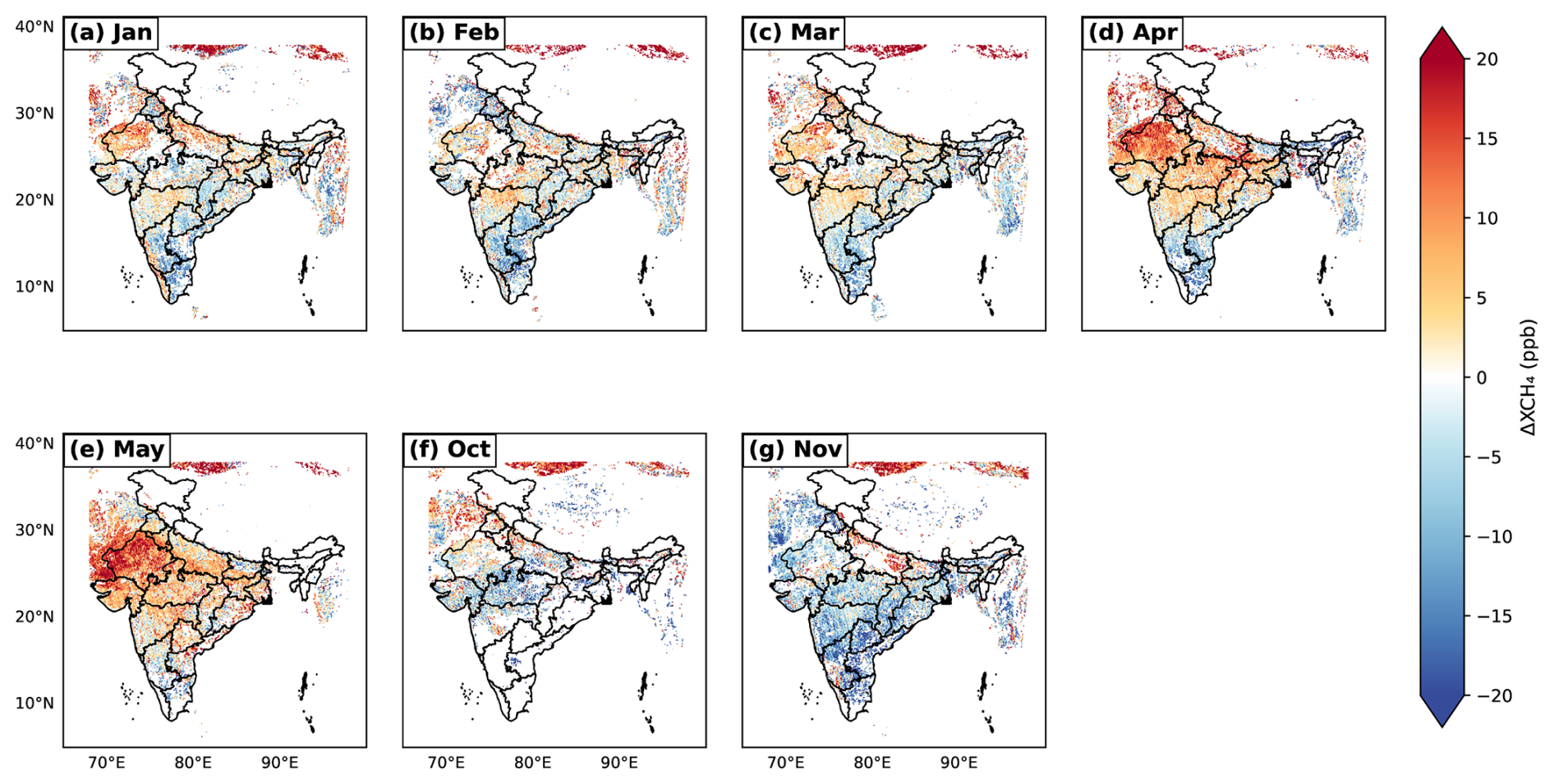
Figure 11 Spatial distribution of the difference between TROPOMI retrievals of XCH₄ (WFMD – Operational) for different months of 2019. Some months are omitted due to poor data coverage caused by filtering based on cloud pixels.

We analyzed three TROPOMI XCH₄ products: scientific (Schneising et al., 2023), operational (Copernicus Sentinel-5P, 2021), and GOSAT-blended (Balasus et al., 2023). The results are presented in Figs. 11 and S14–S16. The above product comparison indicates that differences among these datasets over the region lie mostly in the range of 3 to 6 ppb at the monthly scale. Figure 11 also indicates smaller spatial differences among these products across the Indian region. While these differences do not exceed the unresolved modeling errors, they can still influence inverse estimates, especially when fluxes are retrieved at finer scales. In our inverse setup as well, differences in the products can introduce additional uncertainty into estimates. For instance, using the increased measurement uncertainty as explained in Sect. “Estimating optimized CH₄ flux over India”, we find that the national-scale posterior uncertainty for 2018 increases from 3.5 Tg yr⁻¹ in the baseline inversion to 4.4 Tg yr⁻¹. While the mean posterior emission estimates remained unchanged in our case, an increase in posterior uncertainty underscores the importance of addressing differences in satellite retrievals and their error characterization in inverse modeling.

While these mean differences are small across the region, the comparisons indicate considerable variation in spatial coverage between WFMD and Operational data products. For instance, Fig. S15 shows the spatial patterns of XCH₄ using the Operational product, but with comparatively sparse spatial coverage compared to those using the WFMD product (Fig. S14). Our analysis does not account for differences in spatial coverage between products, as illustrated in Figs. S15 and S14. These differences may potentially affect the inverse estimates, and assessing their impact requires further study. A recent study also reveals considerable impacts of differences in retrievals on the inverse-based European CH₄ emission estimates when utilizing those TROPOMI XCH₄ products (Sicsik-Paré et al., 2025). While a detailed performance assessment of different observational products – regarding their coverage, retrieval errors, and spatial inconsistencies – is beyond the scope of this study, we emphasize the necessity to investigate the robustness of satellite-based inversions considering these differences, particularly at a finer scale. This focused approach will thus pave the way for more consistent emission estimates.

Although we utilize high-density, high-quality, and high-resolution TROPOMI satellite retrievals together with a high-resolution transport model, our inversion algorithm is limited by its dependence on the spatial distribution of emissions in prior inventories. Our optimization adjusts the magnitude of prior emissions over the target region by utilizing additional information from independent measurements, but the present inverse modeling design has the limitation to minimize any flux errors in the sub-scale spatial distribution. However, we expect that those spatial errors may have a minor impact on our annual national estimates owing to our temporal and spatial averaging. We also acknowledge that the resolution of the retrieved emissions (as defined by state vectors) is a limitation when considering the information content that can be deduced from TROPOMI observations. For instance, Sicsik-Paré et al. (2025) demonstrated inversions over Europe using TROPOMI observations to retrieve fluxes at 0.5° × 0.5° resolution. The above-mentioned limitation of the present study stems from the region being undersampled and understudied against independent observations, as well as the need to address the risk of inferring overly confident flux retrievals. To retrieve the maximum information content from TROPOMI observations without compromising the accuracy of the retrieved fluxes, further improvements in the demonstrated inversion strategy are required. This includes adequate characterization of both forward model and observational errors against independent observations, as well as conducting sensitivity tests to examine the representativeness of observations to retrieve high-resolution fluxes. The above tasks thus warrant increased observational coverage and advanced inverse modeling techniques that properly account for such errors and sensitivities, which are currently limited over the region, not addressed in the study; thus, demand a future investigation in this direction.

The present analysis excluded wetland emissions from the optimization due to their negligible contribution to column enhancements. This is demonstrated in Figs. S9 and S10, which show that the simulated wetland emission enhancements in the column are significantly smaller than anthropogenic enhancements. As a result, TROPOMI observations cannot be utilized with our model setup to reliably differentiate wetland emission signals for accurate wetland emission estimates. Approximately 7.5 Tg wetland CH₄ emissions from the Indian region were reported in the Global Methane Budget 2000–2020 (Saunois et al., 2025). Janardanan et al. (2024) used wetland prior emissions from the Global Methane Budget 2000–2017 (Saunois et al., 2020) in their inversions and reported approximately 3.8 ± 0.16 Tg CH₄ emissions annually from Indian wetlands. At the same time, the BUR4 report (MoEFCC, 2024) has not included the wetland emission estimates, possibly due to inadequate data coverage. Bernard et al. (2025) also discussed the limitations in modeling the wetland emissions from the tropical region due to the inadequacy of available measurements. The above level of estimation discrepancies calls for a country-specific wetland inventory that can also be used as reliable prior fluxes in future inverse modeling. Also, there could be a possible overlapping of natural and anthropogenic (agricultural fields) wetlands in the emission inventories used, which may overestimate the sectoral contribution of posterior fluxes (Zhang et al., 2014).

Another limitation could be that though the GFAS inventory includes agricultural residue burning, small fires that are common in smallholders for clearing the wastes and field preparation can be missed from prior inventories, as reported in Deshpande et al. (2022). Also, in this study, our focus is restricted to providing national-scale anthropogenic CH₄ emission estimates. While the inversion framework in principle allows for analysis at finer spatial or sectoral scales, here we intentionally report only the aggregated national totals, as our aim is to evaluate the feasibility of TROPOMI-WRF-GHG for constraining India's methane budget. A more detailed exploration of sectoral and regional signals is left to future work with more coverage of observations and the implementation of more advanced inverse modeling methods.

4 Conclusions

In this study, we investigate the potential of TROPOMI satellite observations along with a high-resolution atmospheric transport model, WRF-GHG, to represent the distribution of CH₄ emissions over the Indian region. Analysis of the bottom-up inventories shows enteric fermentation as the most significant contributor to CH₄ emissions in India (42.9 %), followed by wastewater treatment (19.2 %), agricultural soil (12.4 %), fuel exploitation (6.7 %), and wetlands (5.2 %, excluding agriculture). The above proportions highlight the considerable impact of anthropogenic sources on CH₄ accumulation in the atmosphere. As expected, CH₄ emissions from rice agriculture (August), wetlands (July), and biomass burning (March) exhibit distinct seasonal patterns. The bottom-up anthropogenic CH₄ emissions, and consequently the total atmospheric XCH₄ mixing ratios, have shown some peaks over South India due to a few prominent emission hotspots. This study characterizes regional and seasonal methane-emission patterns from global bottom-up inventories and assesses their possible influence on XCH₄ enhancements. The analysis identifies key uncertainty drivers such as the elevated anthropogenic emissions in the post-monsoon months, thereby guiding refinement of top-down CH₄ estimates across India.

The WRF-GHG simulations of XCH₄ mixing ratio enhancements indicate considerable contributions from anthropogenic and biomass burning emissions, particularly in the IGP region (from 27 to 67 ppb). The highest seasonal enhancements of anthropogenic XCH₄ occur during winter, influenced by agricultural emissions, biomass burning, and atmospheric winter transport. This inference aligns with previous studies (e.g. Patra et al., 2011) that show stronger vertical mixing during the summer, associated with higher boundary layers and faster wind speeds, may impact CH₄ columns. Both the observed and modeled total XCH₄ show significant peaks over the IGP region, with values ranging from ∼ 1862 to ∼ 1870 ppb during October–November. Though WRF-GHG remarkably captures atmospheric XCH₄ patterns, simulations generally overestimate XCH₄ levels compared to TROPOMI. The total XCH₄ along the eastern coast reflects the influence of agricultural soil emissions on column-averaged methane. Although wetland emissions peak in this region, their contribution to atmospheric mixing ratios is negligible. Our high-resolution model is capable of capturing surface CH₄ variability, especially for the well-mixed conditions, as confirmed by the ground-based CH₄ observations. However, this comparison is representative of only one station, though it is a complicated measurement location to be represented by the model owing to the influence of coastal meteorology. Such ground-based observations across India are essential for evaluating the full potential of high-resolution models in representing the atmospheric distribution of trace gases and to better constrain vertical transport processes and regional representativeness.

The inversion analysis using our high-resolution model and TROPOMI observations reports an annual mean anthropogenic CH₄ emission budget of 23.4 ± 3.3 Tg yr⁻¹ (excluding biomass burning of 0.3 Tg yr⁻¹). Our estimations are 13 % to 24 % lower than the EDGAR emission estimates. At the same time, our estimate is 19 % higher than what the Government of India reported to the UNFCCC for the same period, but close to the latest Global Methane Budget 2000–2020.

We emphasize the critical need for robust reporting of CH₄ emissions from the Indian region in global emission inventories. Achieving this requires an enhanced network of ground-based atmospheric trace gas measurements and advancements in satellite capabilities, alongside advanced modeling techniques with adequate model error characterization. With the above expansion, future research can decisively explore and evaluate various inverse techniques. By implementing methods such as the Ensemble Kalman Filter (EnKF) and 4D Variational Inversion (4D-Var), we can effectively manage highly resolved state vectors, leading to significantly improved emissions data at much finer scales over India. Additionally, we recommend inter-comparisons of TROPOMI-based inversions using various inversion frameworks and transport models over India, with the aim of identifying biases in the forward models and the inversion frameworks. Further, we encourage rigorous sensitivity testing with TROPOMI inversions to assess the robustness of derived emissions, particularly with respect to differences in satellite products, coverage and sampling, as these factors can significantly influence inverse-based estimates. Overall, our analyses highlight that TROPOMI observations can provide valuable insights into CH₄ emissions, and the WRF-GHG model has the potential to be used in an assimilation system to refine emissions.