Long-term analysis of atmospheric propane over Southern Europe based on observations conducted at the WMO-GAW station of Monte Cimone

This study presents the analysis of a 13-year time series of continuous measurements of propane (C₃H₈) from the WMO-GAW station of Monte Cimone (CMN, Italy) between 2011 and 2023. Background trend and pollution events are evaluated to establish how this remote site is influenced by regional and/or global emissions. Over the study period, C₃H₈ background mixing ratios exhibited a significant decrease of −3.8 [−5; −2.3; 95 % confidence interval] ppt yr⁻¹. C₃H₈ seasonal amplitude showed a significant decrease of −6.2 [−7.4; −5.1] ppt yr⁻¹ in the study period, driven by a reduction in winter emissions. Based on back-trajectory sensitivity analysis, CMN and Jungfraujoch (JFJ, Switzerland) were found to be predominantly influenced by air masses originating from the central European continent and the western Mediterranean basin. Using the 2022 observations of CMN and JFJ stations, and the Flexpart-Flexinvert inverse modeling framework, we estimated the distribution of regional emissions and compared it with the EDGAR bottom-up emission inventory. In particular, for Italy and France, prior emissions of C₃H₈ were underestimated approximately by a factor of 2, likely due to overlooked C₃H₈ emissions sources and/or inaccurate activity data used to compile the bottom-up inventory.

1 Introduction

Atmospheric propane (C₃H₈) can affect both climate and air quality through the formation of tropospheric ozone and carbonyl compounds, eventually leading to secondary organic aerosols (Rosado-Reyes and Francisco, 2007). According to Hodnebrog et al. (2018), the specific radiative forcing for the indirect effects of C₃H₈ is about 99 % of its total specific radiative forcing through interactions with O₃ formation and CH₄ removal. Previous studies (Helmig et al., 2016; Angot et al., 2021; Li et al., 2022; Toon et al., 2021) informed about variations in the trends of the C₃H₈ mixing ratio in the northern hemisphere in the second decade of this century, with changes in the mixing ratio depending on the location with respect to the main sources of anthropogenic emissions, the time range considered and the sampling region (upper troposphere vs. lower stratosphere). Variations in C₃H₈ mixing ratios were reported with seasons (Helmig et al., 2015) and latitude (Helmig et al., 2014, 2016) at remote measurement stations.

Propane emissions result from natural gas and oil activities (Lan et al., 2019) due to fugitive emissions, the practices of gas venting and flaring (https://www.worldbank.org/en/programs/gasflaringreduction/methane-explained, last access: 2 March 2026), offshore oil loading (Riddick et al., 2019), as well as burning of agricultural residue (Joshi et al., 2024). Several articles (Dalsøren et al., 2018; Bourtsoukidis et al., 2020; Rowlinson et al., 2024; Ge et al., 2024; Tzompa‐Sosa et al., 2019) suggested that missing sources of anthropogenic C₃H₈ emissions (oil and gas activities) or geologic origins could explain the bias between modelled and observed mixing ratios. According to Derwent et al. (2017), the estimates of C₃H₈ emissions from natural gas leakage were biased low in the UK national emission inventory. For the Arabian Peninsula, the discrepancies between the modelled and observed non-methane hydrocarbons may be explained by the degassing of C₃H₈ from the northern Red Sea with emissions comparable to those of the Middle East countries (Bourtsoukidis et al., 2020). Several articles (Lyon et al., 2021; Thorpe et al., 2023; Serrano-Calvo et al., 2023) associated a general decrease in anthropogenic emissions from oil and gas activities in North America with the COVID-19 pandemic and the related economic crisis.

The Mediterranean basin is one of the climate change hotspots due to the consistent number of observed impacts related to climate change and the projected hazards, vulnerability, and risks associated with future scenarios of global increase in temperature (Ali et al., 2022). Therefore, it is urgent to study atmospheric composition in relation to climate-altering compounds and their precursors. This paper aims to analyse the causes that affect the background values of propane in the South European troposphere.

The analysis is based on a 13-year time series of continuous measurements of C₃H₈, carried out at the Italian Climate Observatory 'Ottavio Vittori, a research infrastructure managed by the Institute of Atmospheric Sciences and Climate (ISAC) of the National Research Council (CNR) of Italy, within the framework of the European Research Infrastructure ACTRIS (Aerosol, Clouds, and Trace Gases), dedicated to the observation and understanding of short-lived atmospheric constituents and their interactions. Continuous measurements of CO and CH₄ at the same site are also carried out in the framework of the Integrated Carbon Observation System Research Infrastructure (ICOS-RI). The location of this observatory allows for the study of the evolution of C₃H₈ mixing ratios in the free troposphere of the Mediterranean basin and the emission sources located in the Po Valley. The diurnal and seasonal variability in the C₃H₈ mixing ratios was estimated for the study period. Variations due to the COVID pandemic and high mixing ratio events were analysed. Air mass footprints for CMN were investigated using FLEXible PARTicle (FLEXPART) (Bakels et al., 2024a), a Lagrangian particle dispersion model. The seasonal sensitivity maps of air masses were compared with the sensitivity map calculated for high propane emission episodes.

2 Materials and methods

2.1 Propane, carbon monoxide, and methane datasets

The time frame of this study covered the period from January 2011 to December 2023. In situ online measurements were performed at the World Meteorological Organization's Global Atmosphere Watch (WMO/GAW) global station on CMN (44°12^′ N, 10°42^′ E, 2165 m above sea level). Monitoring of non-methane volatile organic compounds (NMVOC) performed at the CMN station is generally representative of emissions occurring in the European continent as reported by Lo Vullo et al. (2016). Measurements of C₃H₈ were performed with a gas chromatograph-mass spectrometer (GC–MS Agilent 6820 + Agilent 5975C) operating in Selected Ion Monitoring (SIM) mode, preceded by an online sample enrichment using a preconcentration system Unity-2-AirServer-2 (Markes International), following a method described in Maione et al. (2013) and Lo Vullo et al. (2016), according to ACTRIS standard operating procedure (SOP) (https://www.actris.eu/sites/default/files/Documents/ACTRIS-2/Deliverables/WP3_D3.17_M42.pdf, last access: 2 March 2026) and audited under the GAW programme of the WMO by the World Calibration Center for volatile organic compounds in 2018. Real ambient air samples are collected every second hour, alternated with a whole-air calibration mixture (working standard) to correct for short-term instrumental drift, resulting in 12 real air measurements per day. Each month, the working standard is calibrated against a certified “30-compounds Ozone precursor mixture” at a 500 ppt level in nitrogen from the National Physical Laboratory (NPL-United Kingdom). System blanks are evaluated on a weekly basis, with concentrations changing over time but limited well below 15 ppt, with results adjusted accordingly. Total uncertainty for each measurement is calculated as the error propagation of (i) the reproducibility of the repeated working standard runs on the same day, (ii) the detection limit, and (iii) the scale propagation error (derived by the regular NPL/quaternary standard check, additional details in Appendix F). Final quality control of the dataset is checked yearly by an external reviewer as part of the ACTRIS-EBAS SOP procedures before submission for data release to the EBAS repository. In addition, C₃H₈ observations for the year 2022 from JFJ WMO-GAW global station have been used for atmospheric inversion modeling as described in Sect. 2.5. C₃H₈ measurements at JFJ are carried out within the framework of ACTRIS activities, following the same analytical protocol for CMN but with different instrumentation (i.e. the Medusa-AGAGE setup; Miller et al., 2008; Prinn et al., 2018).

Measurements of CO and CH₄ were performed at CMN according to the methods described in Sect. A.

2.2 Meteorological dataset

The meteorological variables (air temperature, pressure, relative humidity, and wind speed) recorded from January 2011 to December 2023 were analysed. Raw data were averaged over a 1 min period. Between 2011 and 2014, the 1 min data were averaged over 30 min periods. Starting in 2015, they were averaged every hour. For the period 2011–2014, the data can be accessed through the NextData database (http://nextdata.igg.cnr.it:8080/geonetwork/srv/eng/catalog.search#/metadata/787c1a26-b92a-4d7d-9d03-8a2531980c52, last access: 2 March 2026). For the time range 2015–2023, the hourly measurements were downloaded from the EBAS website (https://ebas.nilu.no/, last access: 2 March 2026). Specific humidity (SH) was calculated based on air temperature, pressure, and relative humidity data. Figure B1 shows a clear diurnal trend for SH, wind speed, and temperature irrespective of the seasons. Hourly mean values of wind speed were the lowest between 11:00 and 13:00 UTC (Fig. B1b), whereas hourly mean values of temperature and SH were the highest in the early/mid-afternoon (between 13:00 and 16:00 UTC) (Fig. B1d, f). These figures are in line with previous work by Cristofanelli et al. (2021b) who investigated variations in wind speed, SH, and CO ambient levels as proxies of wind regime and vertical transport at CMN. The diurnal variation of SH specular to that of the wind speed may be related to the vertical transport/advection of air masses from the planetary boundary layer at CMN (Cristofanelli et al., 2016) between spring and autumn (Cristofanelli et al., 2015).

2.3 Statistical analysis

To evaluate seasonal cycle and trend, curve fitting of the propane dataset was performed according to the curve fitting method for CO₂ measurements (https://www.esrl.noaa.gov/gmd/ccgg/mbl/crvfit/crvfit.html, last access: 14 October 2024), as done in previous studies on non-methane hydrocarbons by Angot et al. (2021) and Helmig et al. (2014). The curve fitting is performed on the daily mean mixing ratios with at least eight out of twelve measurements. The curve fitting is based on a function fit to the data with a second-degree polynomial function for long-term growth and a four-harmonic series for the annual oscillations. To account for interannual and short-term variations, the filtering of residuals is based on a fast Fourier transform according to Thoning et al. (1989). The trend consists of the polynomial part of the function fit together with the filtered residuals with the seasonal cycle removed, and the long-term cutoff value of 667 d. The smoothed curve is obtained by combining the harmonic components and the residuals from the filter with a short-term cut-off value of 60 d. Following previous studies (Angot et al., 2021; Dlugokencky et al., 1997), for each year, the amplitude (peak-to-trough) of C₃H₈ seasonal cycle was calculated as the difference between the maximum and minimum values of the smoothed curve (red line in Fig. 2) according to the analysis of the first derivative of the smooth curve. The seasonal cycle and trend calculations were done on bootstrap-resampled subsets consisting of 90 % of the daily mean values for 50 iterations. Long-term trends, including the trend of the smoothed long-term curve (Sect. 3.1) and the trend of seasonal amplitudes (Fig. 4), were estimated using Theil-Sen regression, implemented via the scikit-learn Python package (Pedregosa et al., 2011). Statistical significance was assessed using the Mann-Kendall test, implemented via the pyMannKendall Python package (Hussain and Mahmud, 2019), with trends considered significant at p<0.05.

2.4 Sensitivity to air masses starting at CMN

The source-receptor relationship (also referred to as sensitivity) of air masses arriving at CMN was calculated using FLEXPART v11 (Bakels et al., 2024a). FLEXPART simulated the backward transport of virtual air tracer particles released from the receptor site, using wind fields from the European Centre for Medium-Range Weather Forecasts (ECMWF) ERA5 reanalysis. The sensitivity of the receptor to each grid cell is based on the average time that air parcels, traced backward from the receptor, spend in that cell. Only the sensitivity within the model height of 0–500 m was included in the calculation, based on the assumption that emissions primarily occur near the ground within this layer. 10 000 particles were released every 3 h from CMN (44.12° N, 10.42° E, 2000 m a.s.l.) and tracked backward in time for 5 d over the global domain. FLEXPART was driven by ERA5 reanalysis data with a horizontal resolution of 0.5° (Copernicus Climate Change Service, 2018). Sensitivity calculations were conducted for the year 2022, during which the mean seasonal fetch regions were derived and are presented in Fig. 7. The choice of 2022 was motivated by the presence of multiple high-mixing ratio episodes that persisted for more than 2–3 d across various seasons. These prolonged episodes provided sufficient temporal coverage and variability, making 2022 a representative year for analysing the transport patterns and potential source regions influencing observations at CMN.

2.5 Emission estimation using atmospheric inversion method

The inversion of C₃H₈ emissions for 2022 was conducted using the FLEXPART-FLEXINVERT Bayesian inversion framework. In brief, FLEXINVERT (Thompson and Stohl, 2014) Bayesian inversion optimises the emission fluxes constrained by atmospheric observations, a priori inventories, and the atmospheric transport model, accounting for their respective uncertainties. To improve the sensitivity and representativeness of the inversion, propane data from CMN were complemented with measurements performed at JFJ and were assimilated into the inversion. Annadate et al. (2023) observed a decrease in the uncertainties of posterior emission fluxes by adding more observations from different receptors for inversions of a fluorinated trace gas over the European domain. The FLEXPART-FLEXINVERT inversion system has been previously implemented, validated, and extensively used for long-lived compounds such as hydrofluorocarbons using observations from CMN and JFJ (Annadate et al., 2023, 2025).

The primary objective of the inversion process is to obtain an optimised distribution of gridded emissions that reconciles observed atmospheric mixing ratios by minimising the disparity between observed and simulated values, constrained by the uncertainty ranges of the prior state variables. Within the Bayesian framework, assuming Gaussian uncertainty distributions, this optimised state is achieved by minimising the following cost function:

$$\begin{array}{}\text{(1)}& \begin{array}{rl}J\left(\mathit{x}\right)& ={\displaystyle \frac{\mathrm{1}}{\mathrm{2}}}{\left(\mathit{x}-{\mathit{x}}_{\mathrm{b}}\right)}^T{\mathbf{B}}^{-\mathrm{1}}\left(\mathit{x}-{\mathit{x}}_{\mathrm{b}}\right)\\ & +{\displaystyle \frac{\mathrm{1}}{\mathrm{2}}}{\left(\mathit{y}-\mathbf{H}\mathit{x}\right)}^T{\mathbf{R}}^{-\mathrm{1}}\left(\mathit{y}-\mathbf{H}\mathit{x}\right)\end{array}\end{array}$$

where x is the state vector of emissions to be optimised, x_b is the prior emission vector, B is the prior error covariance matrix, R is the observation error covariance matrix, y is the observation vector, and H is the Jacobian matrix relating emissions to observed mixing ratios. A comprehensive description of the error covariance matrices can be found in Thompson and Stohl (2014). In our reference inversions, B is formulated by assigning 100 % uncertainty to the prior emission flux in each grid cell, with spatial correlation lengths of 250 km over land and 1000 km over the ocean. The cost function minimisation is performed using the M1QN3 quasi-Newton algorithm in FLEXINVERT+ based on Gilbert and Lemaréchal (1989), which employs a limited-memory L-BFGS approach. Posterior uncertainty is estimated using a 20-member Monte Carlo ensemble, wherein random perturbations, that are sampled from B and R, are applied to the prior emissions and observations, respectively.

In this study, bottom-up C₃H₈ emissions from the EDGARv8.1 inventory (https://edgar.jrc.ec.europa.eu/index.php/dataset_ap81, last access: 2 March 2026) were used as the prior. EDGAR provides annual, sector-specific gridded fluxes for power generation, industrial combustion, buildings, transport, agriculture, fuel exploitation, industrial processes, and waste, which were aggregated to form the prior flux field for the inversion. Background mixing ratios for CMN and JFJ were estimated following Stohl's method (Stohl et al., 2009), which used FLEXPART sensitivities and prior emissions. Detailed description of Stohl's method, implementation, and comparison with other background estimation methods can be found in Stohl et al. (2009) and Vojta et al. (2022).

For the inversion, observations from CMN and JFJ were aggregated to a 3-hourly temporal resolution. Fixed 3 h time bins (e.g., 00:00–03:00 and 03:00–06:00 UTC) were defined, and all observations within each bin were averaged and assigned to the bin start time. If a bin contained only a single observation, that observation was assigned to the corresponding bin start time. FLEXPART sensitivities were computed at the same 3-hourly intervals by releasing 10 000 particles and tracking them backwards in time for 10 d. Considering the short lifetime of propane, OH reactivity was included in the model. Chemical loss due to reaction with the OH radical is represented in FLEXPART as a first-order linear process. The corresponding mass loss, m, is calculated at each timestep as:

$$\begin{array}{}\text{(2)}& m(t+\mathrm{\Delta }t)=m\left(t\right)e^{\mathrm{-}\mathit{\kappa }\mathrm{\Delta }t}\end{array}$$

where the temperature-dependent reaction rate constant, κ [s⁻¹], was expressed as:

$$\begin{array}{}\text{(3)}& \mathit{\kappa }=C{T}^N{e}^{\mathrm{-}D/T}{C}_{\mathrm{OH}}\end{array}$$

with T being the absolute temperature and C_OH the hourly OH concentration. The reaction constants C, D, and N were chosen to be $\mathrm{7.6}\times {\mathrm{10}}^{-\mathrm{12}}$ cm³ molec.⁻¹ s⁻¹, 585 K, and 0, respectively (Atkinson et al., 2006). In FLEXPART, the OH distribution is represented using monthly mean fields at a horizontal resolution of 1° × 1° with 40 vertical levels, derived from the GEOS-Chem model. To incorporate hourly variability, these fields are scaled using the hourly ozone photolysis rate. The adjustment applies a simple parameterisation that accounts for the solar zenith angle under cloud-free conditions, thereby introducing an hourly modulation of OH concentrations (Bakels et al., 2024a).

3 Results

3.1 Seasonal variations, time series and long-term trend in C₃H₈ atmospheric mixing ratio

The highest monthly means of C₃H₈ mixing ratios were measured between January and March, whereas the lowest monthly means of C₃H₈ mixing ratios occurred between June and September (Fig. 1). Variability in C₃H₈ mixing ratios was higher in cold months and lower in hot months (Fig. B2). Our results are in line with previous findings (Helmig et al., 2015, 2016; Debevec et al., 2021) about higher C₃H₈ mixing ratios in winter compared to summer in several remote global sampling sites in the Northern Hemisphere. Seasonal changes in C₃H₈ reactivity with OH (Helmig et al., 2014, 2016) and emission sources (Kim et al., 2015) play a role in the variations in atmospheric C₃H₈ mixing ratios. The main atmospheric sink of C₃H₈ is through the reaction with OH, whose tropospheric abundance is driven by a complex series of chemical reactions involving tropospheric ozone, methane, carbon monoxide, non-methane hydrocarbons, and nitrogen oxides and by atmospheric variables (i.e., solar radiation and humidity) with a seasonal trend (Helmig et al., 2016). Moreover, gas consumption in the EU is higher in the cold months compared to the hot months (Energy, 2025). In addition, liquefied petroleum gas has generally higher ratios of propane/butane in winter compared to summer (Kim et al., 2015) to improve the start ability of engines fueled with liquefied petroleum gas during the cold season (Baek et al., 2022). Hu et al. (2025) reported a seasonal pattern with higher C₃H₈ emissions in winter compared to summer for the O&NG production regions of the United States.

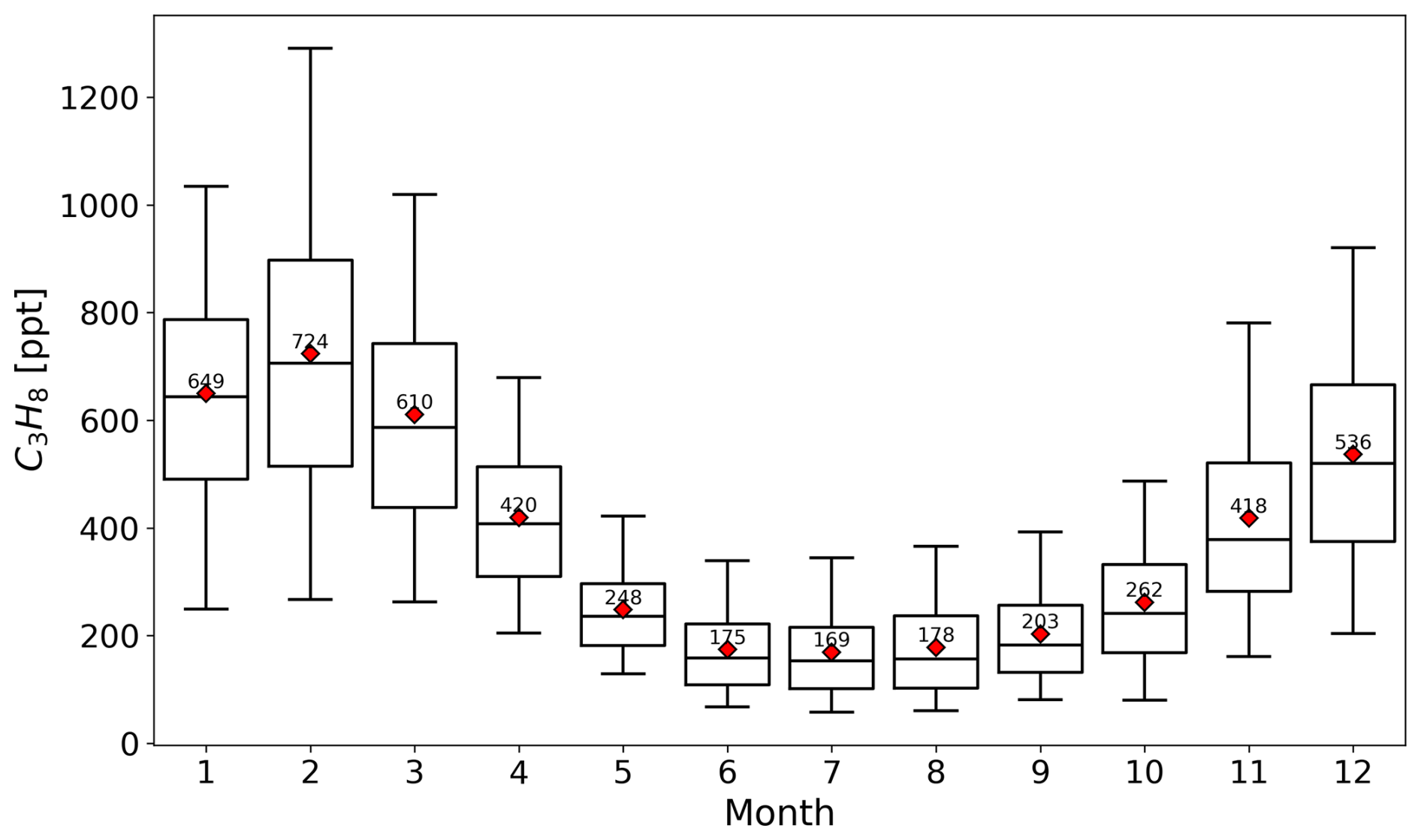
Figure 1 Boxplots of C₃H₈ mixing ratios measured at CMN (Italy) grouped by month from 2011 to 2023. From bottom to top, the horizontal lines of the boxplots show the minimum, 25 %, 50 %, and 75 % percentiles of the data, and the maximum. Red diamonds show mean values.

Figure 2 shows the time series of C₃H₈ hourly and daily mean mixing ratios measured at CMN, and the estimated smooth curve and trend curve from 2011 to 2023. The time series of the C₃H₈ hourly measurements shows a clear seasonal cycle (Fig. 2). Between 2011 and 2023, C₃H₈ mixing ratios exhibited a significant decrease of −3.8 [−5; −2.3; 95 % confidence interval (CI)] ppt yr⁻¹ (solid green line in Figs. 2 and 3). In this study period excluding 2020 because of the pandemic disruption in emissions, the Copernicus Atmosphere Monitoring Service (CAMS) global anthropogenic emission inventory (Soulie et al., 2024) estimated a decrease of about 0.1 Gg yr⁻¹ of C₃H₈ emissions from Europe, whereas European C₃H₈ emissions increased about 4 Gg yr⁻¹ according to the EDGARv8.1 database (Crippa et al., 2024). The trend analysis was also performed on two sub-datasets (i.e., pre-COVID from 2011 to 2019, and post-COVID from 2022 to 2023), to avoid any influences resulting from the drastic changes in activities and emissions during the COVID-19 pandemic, the associated lockdown and recovery phase between 2020 and 2021. Both sub-datasets confirmed a significant decreasing trend. Specifically, the pre-COVID time trend of −2.6 [−4.7; −0.6] ppt yr⁻¹ was comparable to the long-term trend of the full study period.

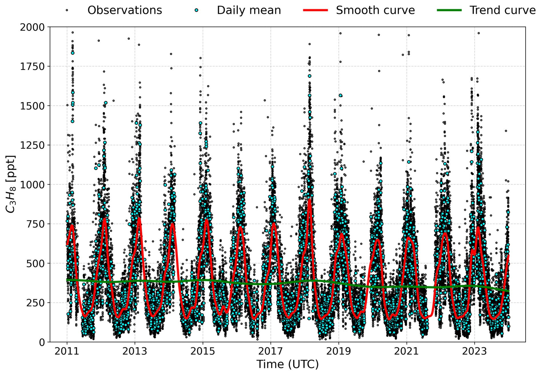
Figure 2 Smooth curve, trend curve, and timeseries of propane hourly and daily mean mixing ratios measured at Monte Cimone (Italy) from 2011 to 2023.

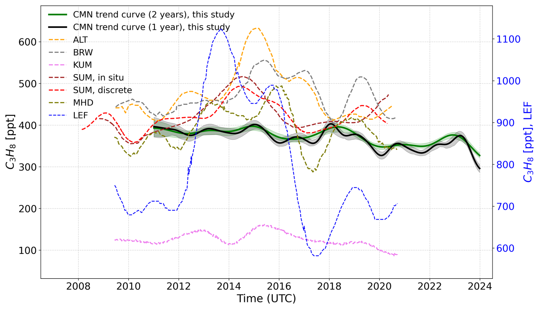
Figure 3 Comparison of the trend curve of propane mixing ratios measured at CMN (CMN, Italy) (solid lines) with those reported by Angot et al. (2021) (dashed lines). Secondary y axis (blue colour) shows values for LEF station. Shaded lines show 95 % confidence interval for CMN trend curves with a long-term cutoff value of 1 or 2 years. ALT – Alert (Nunavut, Canada); BRW – Utqiaġvik, formerly Barrow (Alaska, USA); KUM – Cape Kumukahi (Hawaii, USA); SUM – Summit (Greenland, Denmark); MHD – Mace Head (Ireland); LEF – Park Falls (Wisconsin, USA).

Direct comparison with long-term trends derived from multiple background sites reported by Angot et al. (2021) clearly shows (Fig. 3) an uncorrelated variability among sites, suggesting that the observed year-to-year variations are likely driven by temporal variation in emissions at the hemispheric scale and are not clearly reflected on trends at the global scale.

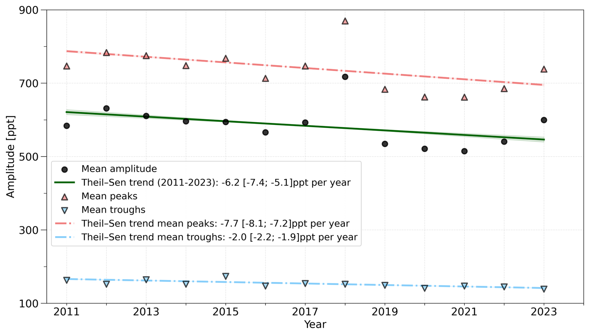
Figure 4 Trend lines of C₃H₈ seasonal amplitudes, and yearly peaks and troughs at CMN (Italy) calculated on the smoothed curve for each year between 2011 and 2023. Shaded lines show 95 % confidence intervals.

Between 2011 and 2023, the trend line of C₃H₈ seasonal amplitudes shows a significant decrease of −6.2 [−7.4; −5.1] ppt yr⁻¹ in the amplitude, with values in the range of 510.5–722 ppt (Fig. 4). Changes in the seasonal cycle of C₃H₈ are affected by emissions, the atmospheric OH sink, and atmospheric transport. Previous studies (Cristofanelli et al., 2021b, a; Vogel et al., 2025) about long term measurements of atmospheric components at CMN did not observe any trends or changes in the transport patterns. Seasonal amplitudes of propane are more sensitive to variations in OH fields during summer seasons, driving summer minima, and to variations in emissions that typically peak during winter/cold periods. The observed reduction in C₃H₈ seasonal amplitude is plausibly explained by a reduction in overall emissions, as pointed out for the long term trend (Fig. 2) affecting mainly winter maxima. The debated (Saunois et al., 2025) positive trend of tropospheric OH concentrations in recent decades reported in a previous study by Liu et al. (2025) may explain the decreasing trend in the summer minima estimated for C₃H₈. The values of amplitudes relative to the peaks were in the range 77.6 %–82.4 %. Based on C₃H₈ measurements in Greenland in the time ranges 2008–2010 and 2012–2020, Angot et al. (2021) reported relative amplitudes in the range of 92 %–96 % and an increase in relative amplitudes of 0.17 % yr⁻¹, although not statistically significant. The removal of C₃H₈ from the atmosphere varies with solar irradiance and thus with the latitude of the measurement station (Helmig et al., 2014, 2016). Therefore, differences in the amplitude of the seasonal cycle of C₃H₈ can be explained by differences in latitudinal locations between this study and the study by Angot et al. (2021). Moreover, the trend in the amplitude of the seasonal cycle of C₃H₈ explained by Angot et al. (2021) as a result of the increase in anthropogenic ON&G activities rather than by biomass burning (BB) emissions or OH sink, could not be a robust explanation for the main behavior recorded for the lower latitude station of CMN.

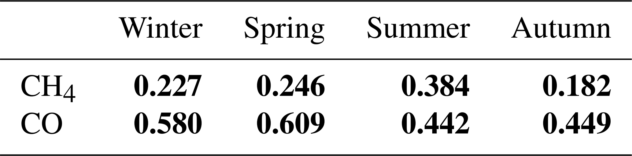
Table 1 shows Pearson's analyses of the hourly mean mixing ratios of C₃H₈, CH₄, and CO measured at CMN from 2011 to 2023. There were statistically significant positive correlations between C₃H₈ and CO, with Pearson correlation coefficients in the range of 0.44–0.61, and the highest values in spring and winter. Statistically significant positive Pearson correlation values were up to 0.38 between C₃H₈ and CH₄. Zhou et al. (2024) reported weak Pearson correlation between column mixing ratios of C₃H₈ and CH₄, resulting from CH₄ emissions related to landfills and livestock farming, whereas a strong Pearson correlation was reported related to shared emission sources such as O&NG activities and fossil fuel (FF) combustion. In summer, BB may be a common source of CO, CH₄, and C₃H₈. The relatively low O&NG extraction activity in the EU compared with the USA suggests that C₃H₈ emissions could be linked to BB and other anthropogenic emission activities such as FF combustion. However, it is important to point out that in summer, CMN can be more exposed to air masses from the regional PBL and that those air masses are probably well mixed once transported to the measurement site. Thus, atmospheric species emitted by different activities at regional scales could be characterized by high temporal correlation.

Table 1 The seasonal Pearson correlation coefficient for the hourly measurements of C₃H₈ with CH₄ and CO from 2011 to 2023. Statistically significant (p<0.05) values are highlighted in bold.

3.2 Diurnal variation in C₃H₈ mixing ratio

The hourly mean values of C₃H₈ mixing ratios were the highest between 14:00 and 16:00 UTC (Fig. 5). Similarly to the annual diurnal variation, the seasonal diurnal variations showed the highest hourly mean values between 14:00 and 16:00 UTC in winter (i.e., December, January, and February) and at 15:00 UTC in the other seasons (i.e., Spring – March, April, and May; Summer – June, July, and August; Autumn – September, October, and November) (Fig. 5). The strong seasonal cycle affects the hourly means of C₃H₈ mixing ratios with the highest values in winter, ranging from 620 to 651 ppt, and the lowest in summer (150 to 210 ppt). Furthermore, the summer season showed the highest variability in diurnal variation of C₃H₈ mixing ratios, with differences (between hourly minimum and maximum) up to 28.8 %, followed by the spring and autumn seasons, with variations of 18.1 % and 12.1 %, respectively. Winter exhibited the lowest diurnal variation, with a maximum difference of only 4.2 %. The difference between winter and summer diurnal variations of airborne pollutants measured at CMN reflects a shift between convective transport from lower altitudes in the daytime and free troposphere conditions at night (Cristofanelli et al., 2016). Moreover, the enhanced OH sink-reactivity during the hot season also contributes to variations between the two seasons (Debevec et al., 2021). During the warm season, CMN is frequently affected by upslope wind intrusions, transporting boundary-layer air from the Po Valley and surrounding regions to the summit (Fischer et al., 2003; Van Dingenen et al., 2005). These intrusions are typically driven by thermally induced mountain-valley circulation and may lead to higher propane mixing ratios during daytime. Upslope intrusions become far less frequent in winter due to reduced surface heating and much shallower boundary layers, hence the lowest diurnal amplitude.

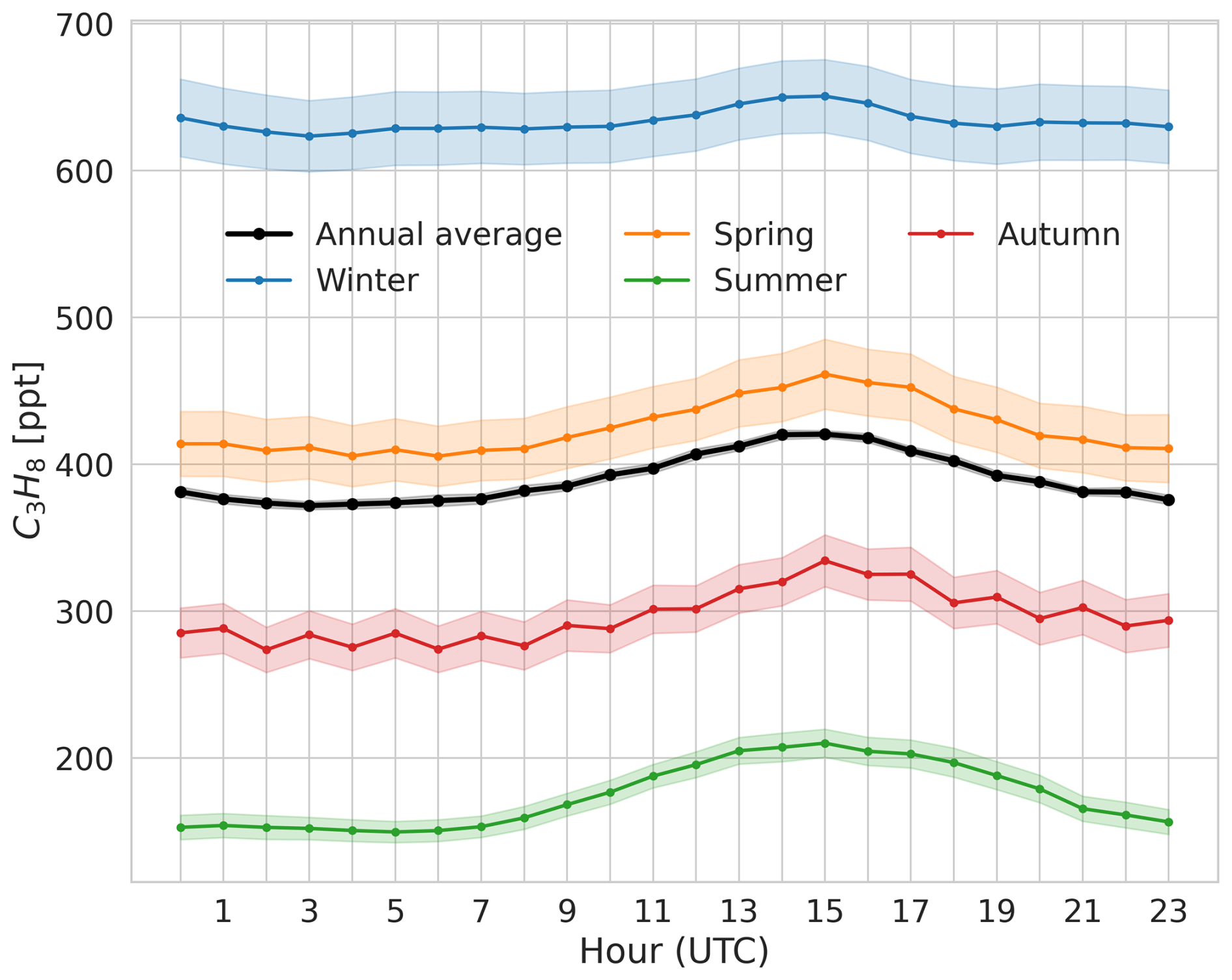
Figure 5 Annual and seasonal diurnal variations of propane mixing ratio measured at CMN (Italy) between 2011 and 2023. Shaded lines show 95 % confidence interval. Smoothing consists of a 3 h centered moving average. Spring – from March to May; autumn – from September to November; winter – from December to February; summer – from June to August.

3.3 Variations in C₃H₈ mixing ratios during the 2020 COVID pandemic

The location of the CMN measurement station also allows one to investigate anomalous variations in atmospheric composition due to unprecedented changes in anthropogenic emission sources such as the COVID pandemic (Cristofanelli et al., 2021a). To investigate potential variations in C₃H₈ mixing ratios during the COVID pandemic in 2020, the mixing ratios measured in 2020 were compared with the pre-COVID (2011–2019), rebound (2021), and post-COVID (2022–2023) periods.

In 2020, the C₃H₈ yearly mean mixing ratios were lower than the mean values before COVID (2011–2019), in 2021 (rebound), and following COVID (2022–2023) (Fig. 6). Kruskal-Wallis (Kruskal and Wallis, 1952) with post-hoc (Games and Howell, 1976) test was applied for testing the null hypothesis that a significant difference exists among the population medians of the groups. This test showed significant (p<0.05) differences between the group means (pre-COVID, COVID, rebound, and post-COVID times) apart from the pairs pre-COVID and rebound, pre-COVID and post-COVID times. Specifically, comparisons of seasonal C₃H₈ mean values showed statistical differences between pre-COVID and COVID both in summer and winter (Fig. C1). The restriction measures were generally set in late February 2020 in Italy and in the following months in the EU. Therefore, the lower mean values of C₃H₈ in winter 2020 compared to pre-COVID are not related to the COVID restrictions in the EU. Witn regard to the lower values in summer 2020, our results align with previous findings that suggested a link between lower emissions of O3 precursors and decreases in O3 mixing ratios measured at CMN (Cristofanelli et al., 2021a) and several high-elevation sites in Europe (Putero et al., 2023). The main drivers of variations in atmospheric C₃H₈ mixing ratios are changes in emission sources, atmospheric chemistry, and transport. Cristofanelli et al. (2021a) observed no substantial variations in the synoptic-scale circulation and vertical transport related to the thermal circulation system at CMN in summer 2020 compared to the previous five years. In this context, the CAMS (Soulie et al., 2024) and EDGARv8.1 (Crippa et al., 2024) inventories estimated that the 2020 anthropogenic emissions of propane from Europe were 91 % and 99.3 %, respectively, of the emissions averaged over the period 2011–2019. In addition, comparisons of aircraft campaign measurements across Europe showed lower OH mixing ratios in the free troposphere during the COVID-19 lockdown compared to previous campaigns (Nussbaumer et al., 2022). The expected longer residence time due to the lower reaction rate between C₃H₈ and OH is therefore at odds with the lower C₃H₈ concentrations recorded at CMN in 2020, which is likely attributable to reduced emissions.

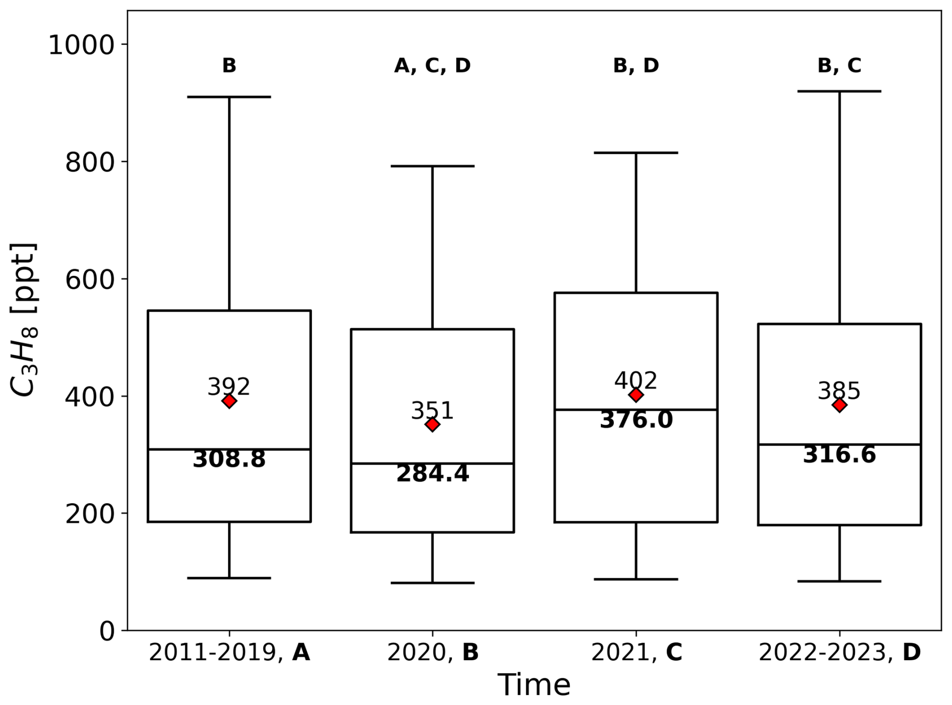
Figure 6 Boxplots of propane mixing ratios measured at Mt. Cimone before COVID (2011–2019, A), during COVID (2020, B), rebound (2021, C), and post-COVID (2022–2023, D). Boxplots show the minimum, 25 %, 50 %, 75 % percentiles of the data, and the maximum. Red diamonds show mean values. Median values are in bold below their respective line. Bold labels report the pairs that have statistically significantly different medians as a result of the pairwise post-hoc test.

3.4 Identification and analysis of events with high C₃H₈ daily mean mixing ratios

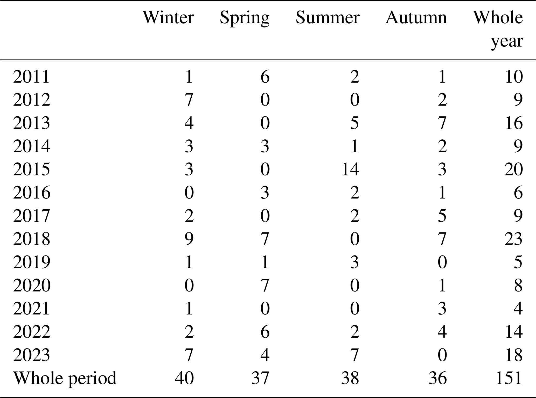
We analysed air mass transport and associated local meteorological variables for selected high mixing ratio episodes. These events with high C₃H₈ mixing ratios were identified as days when the daily mean exceeded the 96th percentile of seasonal daily mean mixing ratios, following Cristofanelli et al. (2021b). The occurrence of events with high C₃H₈ mixing ratios was relatively evenly distributed among the years, apart from 2013, 2015, 2018, and 2023, with 11 %–15 % of the days with high C₃H₈ mixing ratios in the study period (Table 2). Single-day events were from 6 % (in spring) to 25 % (in autumn) of the events with high C₃H₈ daily mean mixing ratios. The events lasting two or more consecutive days were between 6 % (in autumn) and 11 % (in spring) of the events with high C₃H₈ daily mean mixing ratios. Apart from summer, the C₃H₈ high events were characterised by lower air temperature, lower atmospheric pressure, and higher wind speed with respect to the days with ordinary daily mean C₃H₈ mixing ratios (Fig. D1). Cristofanelli et al. (2021b) observed similar atmospheric conditions for NO₂ pollution events recorded at Monte Cimone from 2015 to 2019, suggesting a role of air mass transport triggered by favorable synoptic-scale conditions.

Table 2 Temporal distribution of high C₃H₈ daily mean mixing ratios.

Among the years with the highest number of high-mixing-ratio events, 2022 is the only one with these events in all seasons. As an example of analysis of atmospheric transport of air masses to Monte Cimone during high mixing ratio events, we performed FLEXPART simulations to compute sensitivity to the source regions for the year 2022. Figure 7 presents the mean sensitivity of Monte Cimone to source regions within the study domain for each season in 2022. The seasonal sensitivity patterns show clear differences across the year. Regardless of the season, Monte Cimone was predominantly influenced by air masses originating from the central European continent and the western Mediterranean basin. During winter, the site was affected by long-range transported air masses, with low-sensitivity values extending over a broad area, including parts of North America and Scandinavia. In contrast, summer low-sensitivity regions were more confined, primarily over the Atlantic Ocean and along the western coasts of North Africa. In spring, the station received a greater contribution from air masses originating in Eastern Europe compared to other seasons.

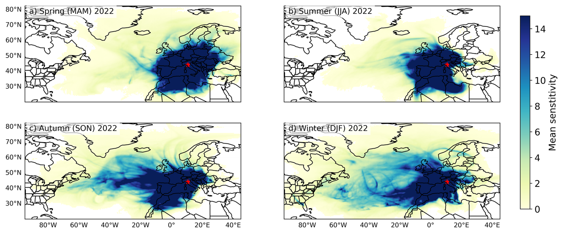
Figure 7 Seasonal mean sensitivity fields indicating the origin of air parcels reaching Monte Cimone (highlighted by a red star), derived by 5 d back-trajectory calculations performed using the FLEXPART model for the year 2022.

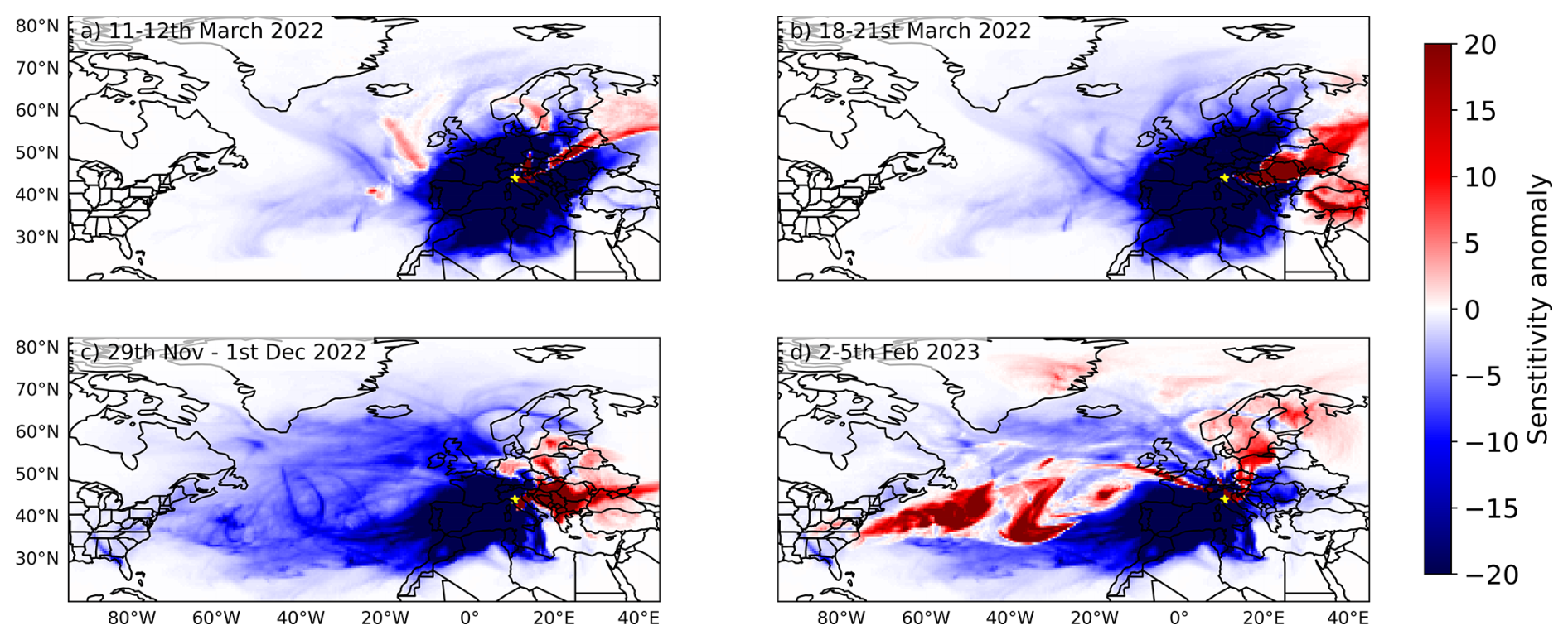
Figure 8 Sensitivity anomaly for four high-mixing ratio propane episodes. The plots show the difference between the sensitivity calculated for the pollution event and the related seasonal sensitivity (Fig. 7).

Figure 8 displays the emission sensitivity (s m⁻³ kg⁻¹) anomalies for four selected high-mixing ratio episodes, relative to the seasonal mean sensitivities (for the corresponding season in which the events occurred). Figure 8a illustrates the anomaly for a 2 d event on 11–12 March 2022. The sensitivity anomaly map shows that the air masses arriving at the station during this period primarily originated from Eastern Europe, Russia, and parts of Scandinavia. Two distinct sensitivity hotspots are also visible over the North Atlantic Ocean for this episode. Figure 8b presents a similar event that occurred on 18–21 March 2022. During this episode, the air masses reaching the station were mainly from Eastern Europe and Russia. Figure 8c shows a 3 d event in winter from 29 November to 1 December 2022. The sensitivity anomalies suggest that southeastern and parts of central Europe significantly influenced the high-mixing ratio episode during this period. Comparisons of time series of hourly means of C₃H₈, CH₄, and CO mixing ratios show a recurring pattern consisting of paired peaks and lows (Figs. D2, D3, D4) for the events characterised by transport of air masses from Eastern Europe and Russia according to the sensitivity anomaly maps (Fig. 8a, b, and c). Figure 8d depicts a 4 d high-mixing ratio event that took place from 2 to 5 February 2023. For this event, the air masses arriving at the station originated from the eastern coast of the United States, the Baltic Sea, and Scandinavia, regions known for their natural gas and oil extraction activities. This event showed a C₃H₈ mixing ratio trend opposite to CH₄ and CO mixing ratios (Fig. D5).

3.5 Inversion estimates

The efficacy of the inversion system was assessed by comparing modelled and observed C₃H₈ mixing ratios at CMN and JFJ for the reference simulation (Fig. 9). The prior mixing ratios show systematic underestimation, with normalised mean bias (NMB) values of −41 % and −47 % at CMN and JFJ, respectively. The inversion substantially improves the agreement, reducing NMB to −3 % at CMN and −14 % at JFJ. A study by Rowlinson et al. (2024), which employed the Community Emissions Data System (https://github.com/JGCRI/CEDS/, last access: 2 March 2026) inventory and the GEOS-Chem model (http://www.geos-chem.org, last access: 2 March 2026) to analyse global VOC emissions in a 2-year period (2016–2017), reported propane prior NMB values of −58 % at CMN and −65 % at JFJ. Their re-speciation approach based on detailed regional NMVOC estimates slightly improved the posterior NMB to −39 % and −43 %. In our analysis, the Pearson's correlation coefficients (R) between observed and prior modelled mixing ratios for the reference simulation were 0.70 for CMN and 0.64 for JFJ, which improved to 0.78 and 0.71, respectively, after the inversion.

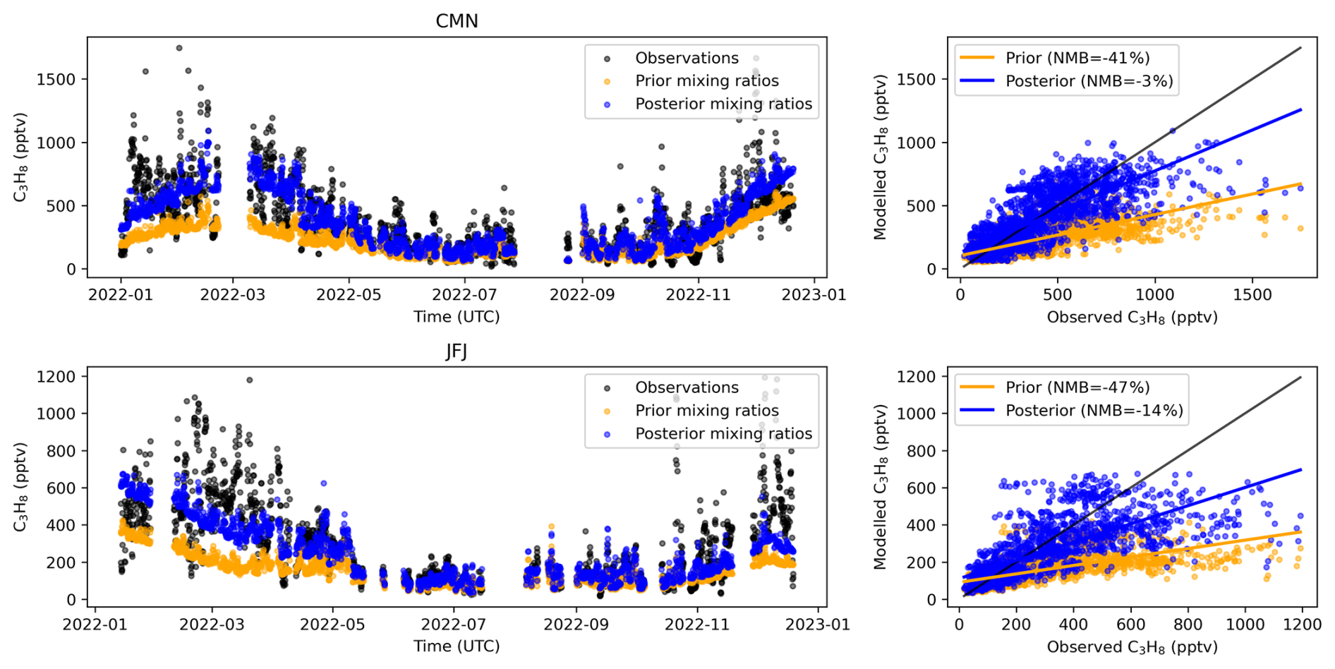
Figure 9 C₃H₈ observed (black) 3-hourly mixing ratios at CMN and JFJ sites compared with prior mixing ratios (orange) and posterior mixing ratios (blue) from the reference inversion.

A sensitivity inversion was conducted with the OH loss term excluded in the FLEXPART transport model to evaluate the influence of chemical oxidation on the posterior emission estimates. In the absence of OH loss, posterior emissions were reduced to less than half of the reference inversion values (Fig. E1), underscoring the critical role of the oxidative sink in the propane budget. It should be noted that an overestimation of OH concentrations would lead to an overestimation of emissions, as the inversion would compensate for the enhanced simulated loss by increasing the source term. Figure E2 shows that the simulated mixing ratios for the reference simulation are lower than those for the simulation without OH loss. While OH fields are subject to uncertainties of approximately 10 %–20 % (Naik et al., 2013; Wolfe et al., 2019) in current chemical transport models, the sensitivity analysis demonstrates that the inversion framework responds appropriately to changes in the chemical loss term, and any systematic bias in OH would propagate linearly into the emission estimates.

Figure 10 illustrates that the prior C₃H₈ emissions are substantially underestimated in the EDGAR inventory. Our inversion yields posterior emissions of 53.4 [47.0–61.2; 90 % CI] Gg yr⁻¹ for Italy, 4.2 [3.3–4.9; 90 % CI] Gg yr⁻¹ for Switzerland, and 54.3 [47.2–60.7; 90 % CI] Gg yr⁻¹ for France. These correspond to increases of 101 % and 149 % over the EDGARv8.1 prior estimates for Italy and France, respectively, posing the question about possible relevant underestimated emissions from some sectors or the likelihood of missing sources in the EDGAR database, such as the captured sources in the south of Italy (Fig. 11), where several of the main petrochemical plants are located. Comparisons of our estimates of propane emissions with the CAMS estimates confirm increases of 71 % and 118 % over the CAMS global anthropogenic emissions inventory (Soulie et al., 2024) for Italy and France, respectively. Similar conclusions were derived by Rowlinson et al. (2024), where improvements based on re-speciation of inventories with detailed regional information were mainly for ethane, leaving some uncertainties for C₃H₈. Previous studies related the observed low estimations of propane emissions at the global (Etiope and Ciccioli, 2009) and regional (Bourtsoukidis et al., 2020) scales to missing geologic sources, and fossil fuel emissions in the USA (Tzompa‐Sosa et al., 2019) or the Northern Hemisphere (Dalsøren et al., 2018). In this context, previous studies (Dalsøren et al., 2018; Tzompa‐Sosa et al., 2019; Rowlinson et al., 2024; Ge et al., 2024) concluded that current emission inventories underestimate anthropogenic fossil fuel emissions of C₃H₈.

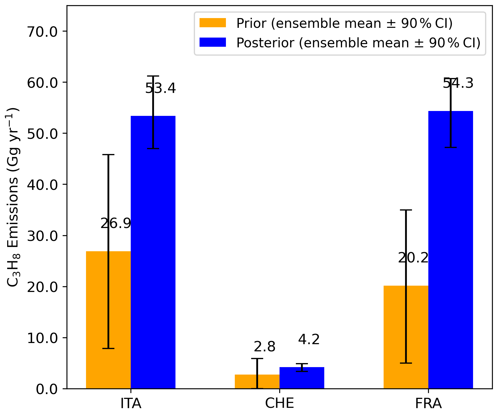
Figure 10 Prior and posterior C₃H₈ emission estimates for Italy (ITA), Switzerland (CHE), and France (FRA). Bar heights represent the ensemble mean of 21 inversions (20 Monte Carlo inversions and 1 reference inversion). Error bars denote the 90 % confidence interval (5th–95th percentile).

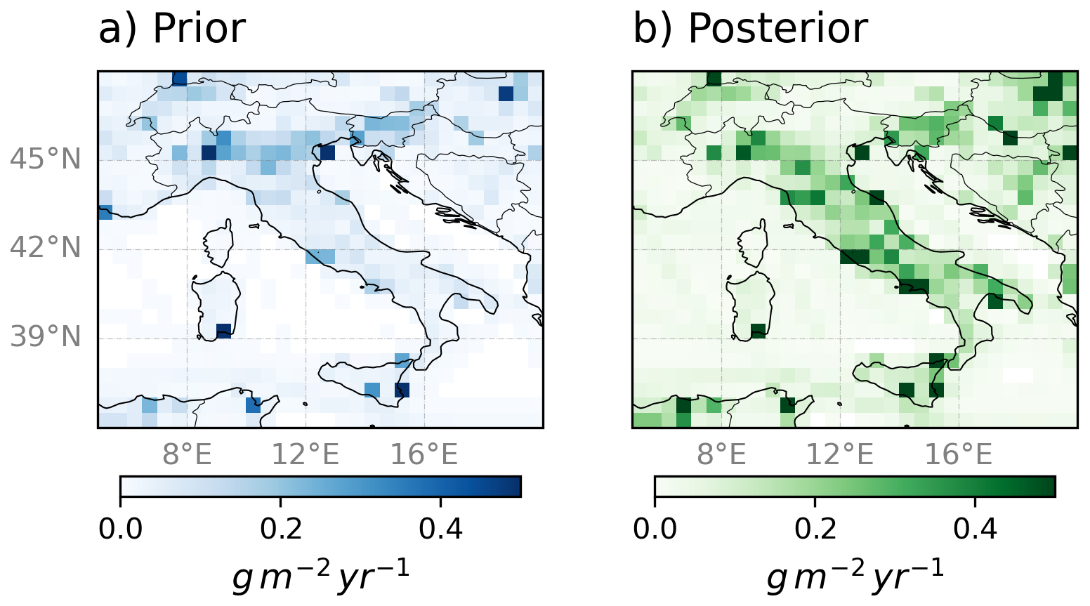
Figure 11 Spatial distribution of prior (EDGARv8.1) and posterior emission flux from the reference inversion of C₃H₈ for Italy for 2022.

4 Conclusions

Propane (C₃H₈) is a key non-methane hydrocarbon with significant implications for tropospheric chemistry, particularly as a precursor to ozone and secondary organic aerosol formation and participating to the global atmospheric oxidative capacity by reacting with hydroxyl radicals, thereby influencing methane lifetime and background ozone levels, with implications for both climate forcing and air quality.

This study presents the analysis of a 13-year time series of continuous measurements of C₃H₈ conducted at the WMO-GAW station of Monte Cimone. Hourly means of C₃H₈ mixing ratios followed a diurnal trend with peaks between 14:00 and 16:00 UTC and a seasonal trend, with the highest values in winter and the lowest in summer. Moreover, the variability in hourly means of C₃H₈ mixing ratios was the lowest in winter and the highest in summer.

In spring and winter, there were strong positive Pearson's correlation coefficients between C₃H₈ and CO, likely due to common anthropogenic emission sources or mixing of anthropogenic sources along the transport path.

Between 2011 and 2023, C₃H₈ long-term trend exhibited a decrease of −3.8 [−5; −2.3; 95 % confidence interval] ppt yr⁻¹.

During the COVID pandemic, C₃H₈ yearly mean mixing ratio was lower than the mean values before COVID (2011–2019), likely due to decreases in anthropogenic emissions.

The amplitude of the C₃H₈ seasonal cycle showed a significant decrease of −6.2 [−7.4; −5.1] ppt yr⁻¹ in the study period, driven by a reduction in winter emissions.

Consistent negative differences between the 2022 prior and posterior emissions of C₃H₈ for France and Italy rose from atmospheric inversion estimates performed for the countries with relatively high sensitivity to CMN and JFJ stations, namely France, Italy, and Switzerland. This suggests revising the EDGAR emissions inventory for overlooked C₃H₈ emissions sources and activities. Also in view of recent disruption in the European energy mix, the estimates of C₃H₈ at the national level should adopt both bottom-up and top-down inverse modeling based on atmospheric measurements methods to underscore the utility of C₃H₈ both as a diagnostic tracer of O&NG emissions and as an indicator of the broader impacts of energy sector practices on atmospheric composition. The results achieved by this work are mainly constrained by the limited availability of the measurement dataset for the European domain. Therefore, it is crucial to put additional effort into the monitoring activities at different scales to further our understanding of the atmospheric abundances and emissions of C₃H₈, its role in the atmospheric chemistry, and its environmental effects.

Appendix A: Carbon monoxide, and methane datasets

From 2011 to 2015, CH₄ and CO observations were carried out using a GC-FID system, designed according to AGAGE protocol for the GC-MD setup. The calibration of the GC-FID system was performed with a set of 6 NOAA calibration mixtures with concentrations spanning the the range of ambient air values. Quality assurance/quality control procedures were done regularly in compliance with AGAGE protocols by means of GCWerks (SIO) software. From 2015 (for CH₄) and from 2018 (for CO), observations have been carried out by using Cavity Ring Down Spectroscopy (CRDS) instruments. From 2018, CO and CH₄ observations have been performed at CMN in the framework of ICOS. Within ICOS, observations are carried out in a standardized way for measurement set-up, used materials, quality assurance strategy, and data creation workflow. (Hazan et al., 2016) and (Yver-Kwok et al., 2021) provided a detailed description of the quality assurance programme for ICOS measurements. CH₄ observations from 2015 to 2017 have been carried out by CAMM – Italian Air Force in the GAW/WMO framework. The quality assurance programme has been designed based on the recommendations provided by GAW/WMO (https://library.wmo.int/idurl/4/69756, last access: 2 March 2026). In particular, a multipoint calibration is performed every 3 months against three laboratory standards provided by NOAA whose mole fractions exceed the range for ambient air. Calibration data are post-processed, and calibration coefficients are derived through linear regression and used to correct the in situ air measurements. A specific water vapour correction determined during a system and performance audit by the WMO/GAW “World Calibration Center for Surface Ozone, Carbon Monoxide, Methane, Carbon Dioxide and Nitrous Oxide” was applied to the data (Zellweger et al., 2020). CAMM operators manually screened the data to remove anomalous events related to instrumental/sampling issues or local emissions.

Appendix B: Monthly statistics

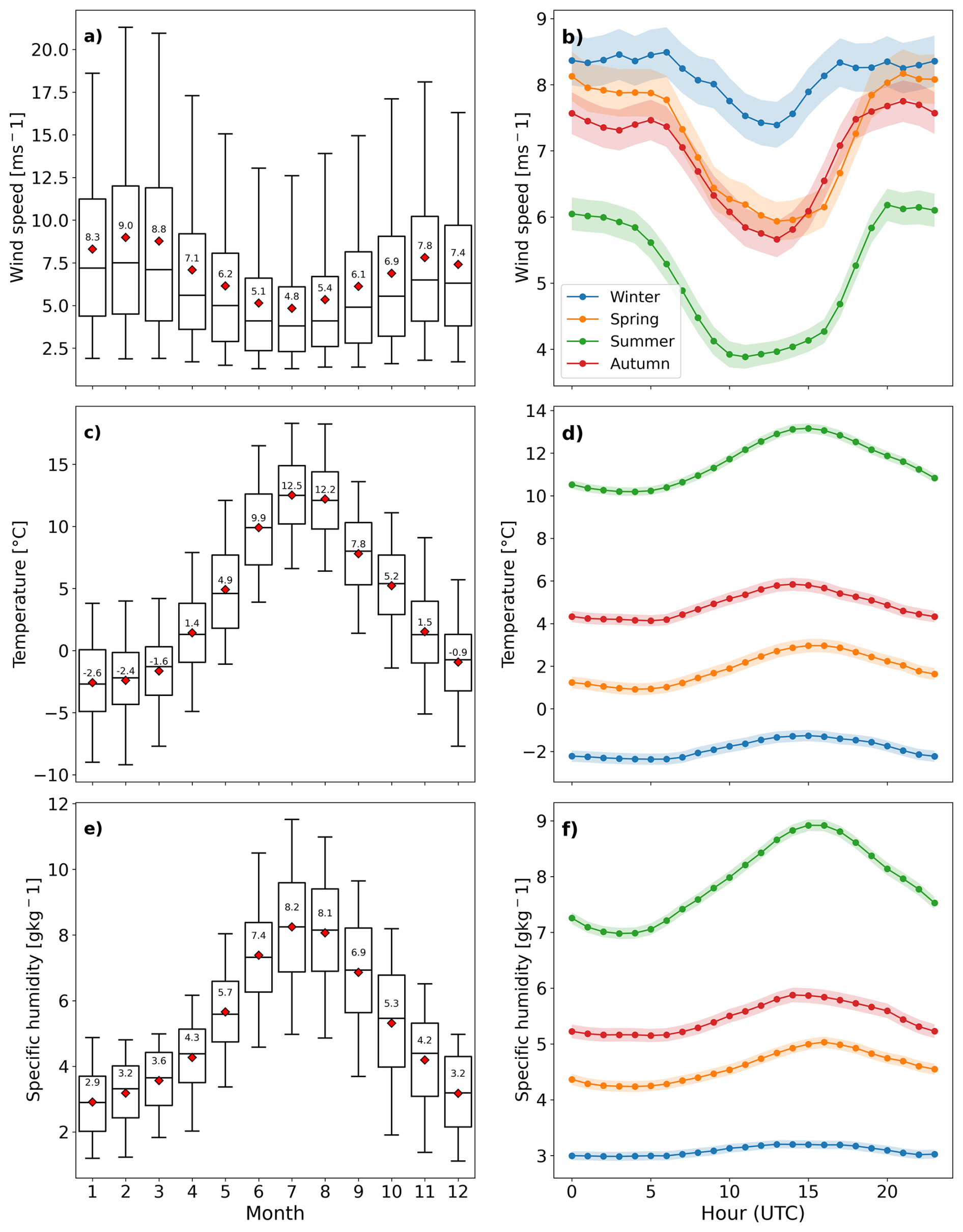
Figure B1 Monthly box plots (a, c, e) and seasonal diel variation (b, d, f) in wind speed (first line), temperature (central line), and specific humidity (third line) at Monte Cimone (Italy) from 2011 to 2023. From bottom to top, the horizontal lines of the box plots show the minimum, 25 %, 50 %, and 75 % percentiles of the data, and the maximum. Red diamonds show mean values. Shaded lines show a 95 % confidence interval. x-axis shows time UTC in panels (b), (d), and (f).

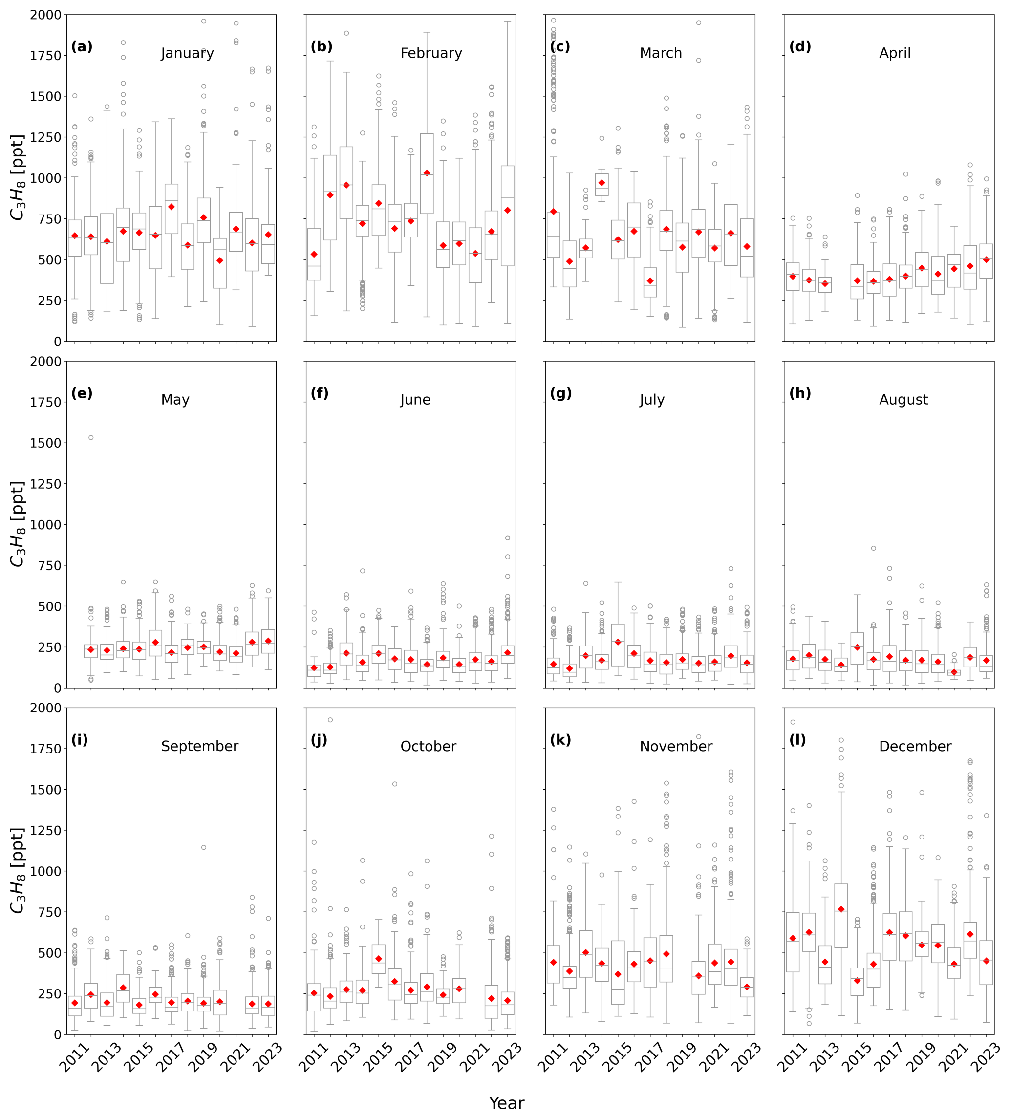
Figure B2 Boxplots of propane concentrations measured at Monte Cimone (Italy) grouped by month from 2011 to 2023. From bottom to top, the horizontal lines of the boxplots show the minimum, 25 %, 50 %, and 75 % percentiles of the data, and the maximum. Red diamonds show mean values. Circles show outliers. Empty spaces in panels (d), (e), (i), (j), and (k) are due to missing data.

Appendix C: COVID – statistics

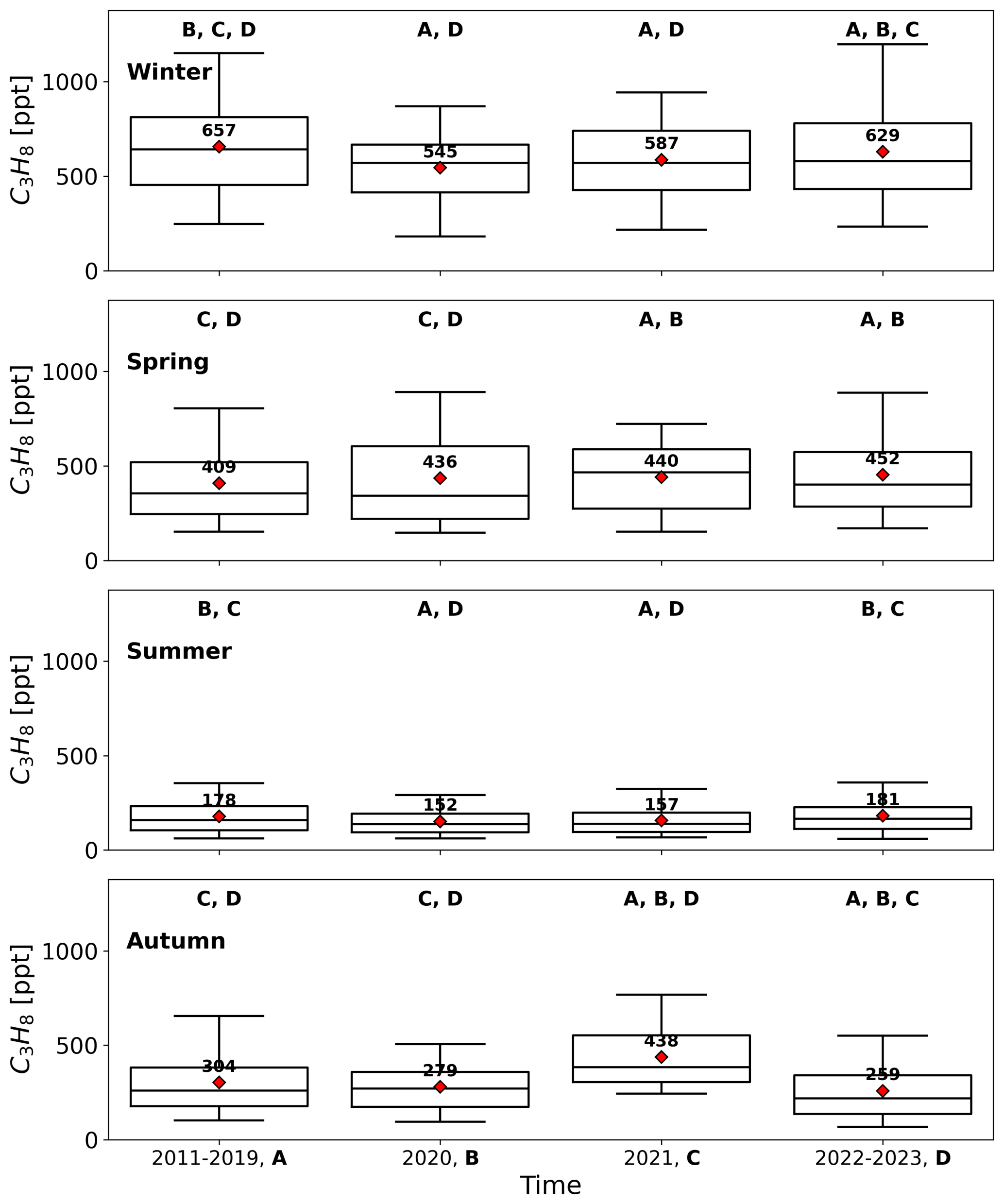
Figure C1 Boxplots of seasonal propane mixing ratios measured at Mt. Cimone before COVID (2011–2019, A), during COVID (2020, B), rebound (2021, C), and post-COVID (2022–2023, D). Boxplots show the minimum, 25 %, 50 %, 75 % percentiles of the data, and the maximum. Red diamonds show mean values. Bold labels report the pairs that have statistically significant different medians as resulted from the pairwise post-hoc test.

Appendix D: Events – statistics

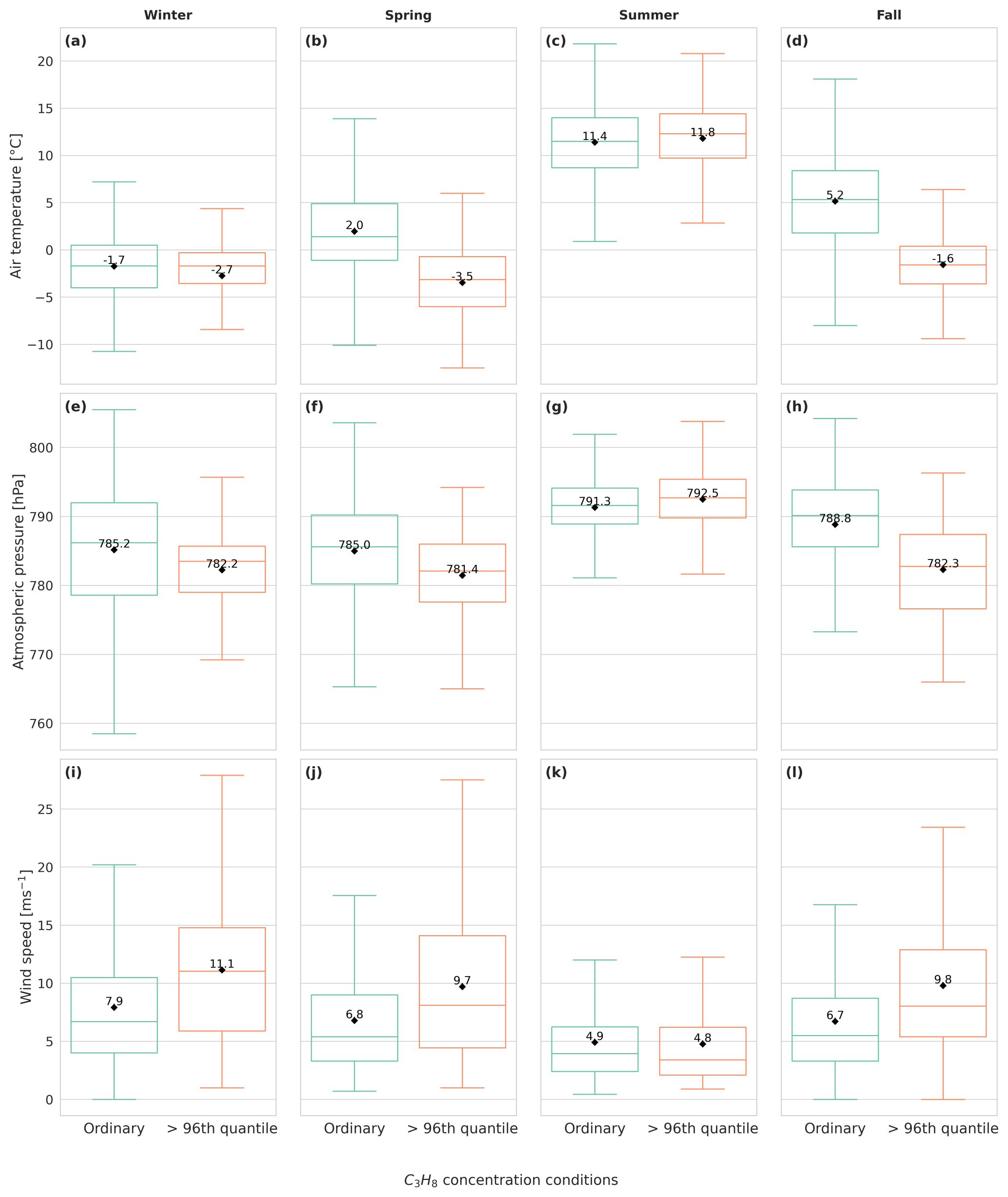
Figure D1 Comparisons between box plots of hourly measurements of air temperature (a, b, c, d), atmospheric pressure (e, f, g, h), and wind speed (i, j, k, l) at Monte Cimone (Italy) grouped by seasons for the ordinary and high C₃H₈ daily mean mixing ratios from 2011 to 2023. From bottom to top, the horizontal lines of the boxplots show the minimum, 25 %, 50 %, and 75 % percentiles of the data, and the maximum. Red diamonds show mean values.

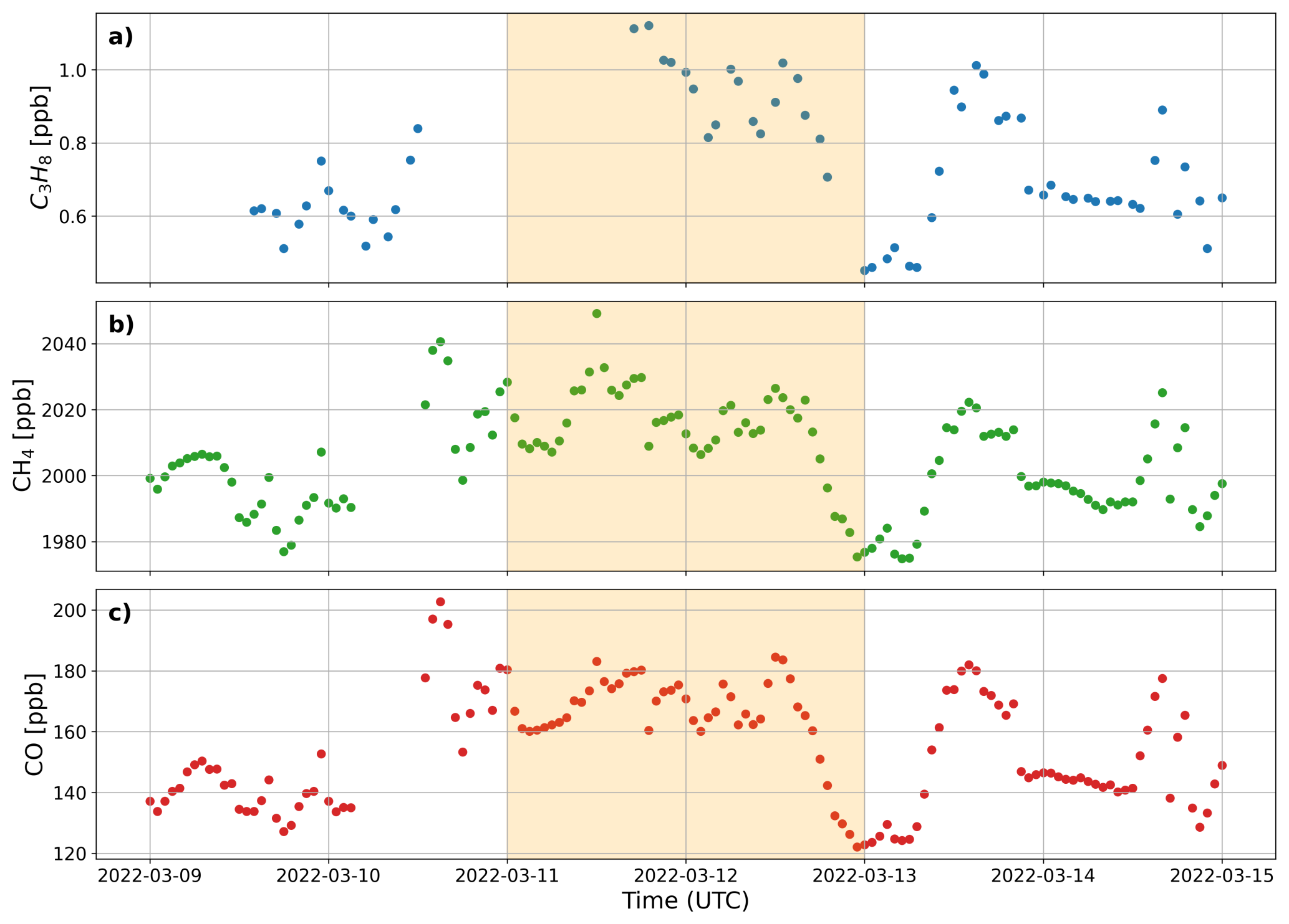
Figure D2 Time series of hourly means of (a) C₃H₈, (b) CH₄, and (c) CO mixing ratios for the event occurring between 11 and 12 March 2022 (orange band) with daily mean C₃H₈ mixing ratios above the 96th percentile of the respective seasonal daily mean percentile.

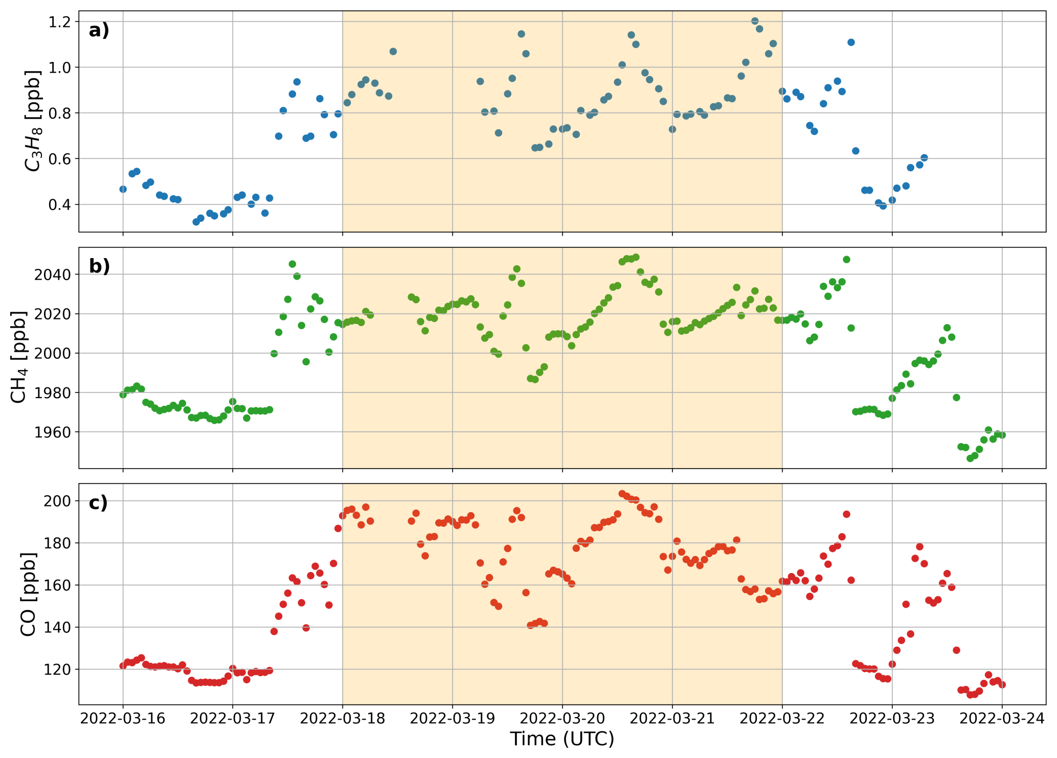
Figure D3 Time series of hourly means of (a) C₃H₈, (b) CH₄, and (c) CO mixing ratios for the event occurring between 18 and 21 March 2022 (orange band) with daily mean C₃H₈ mixing ratios above the 96th percentile of the respective seasonal daily mean percentile.

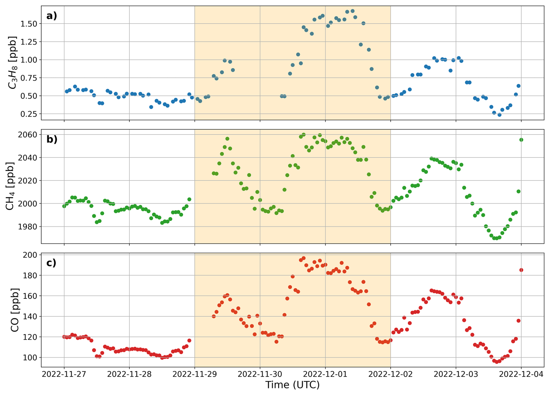
Figure D4 Time series of hourly means of (a) C₃H₈, (b) CH₄, and (c) CO mixing ratios for the event occurring between 29 November and 1 December 2022 (orange band) with daily mean C₃H₈ mixing ratios above the 96th percentile of the respective seasonal daily mean percentile.

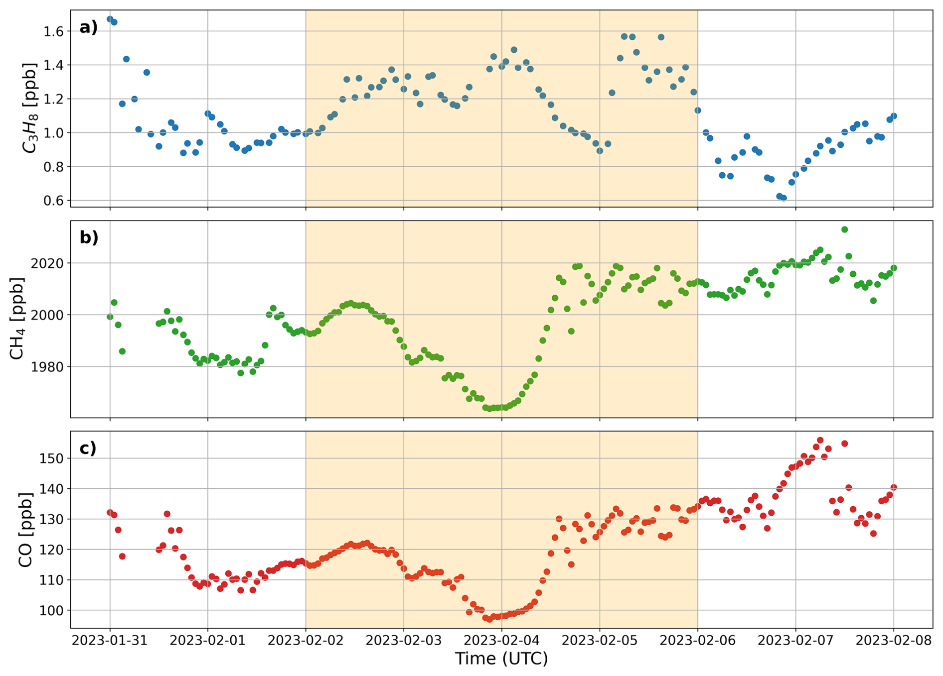
Figure D5 Time series of hourly means of (a) C₃H₈, (b) CH₄, and (c) CO mixing ratios for the event occurring between 2 and 5 February 2023 (orange band) with daily mean C₃H₈ mixing ratios above the 96th percentile of the respective seasonal daily mean percentile.

Appendix E: Uncertainty due to reaction with OH radical

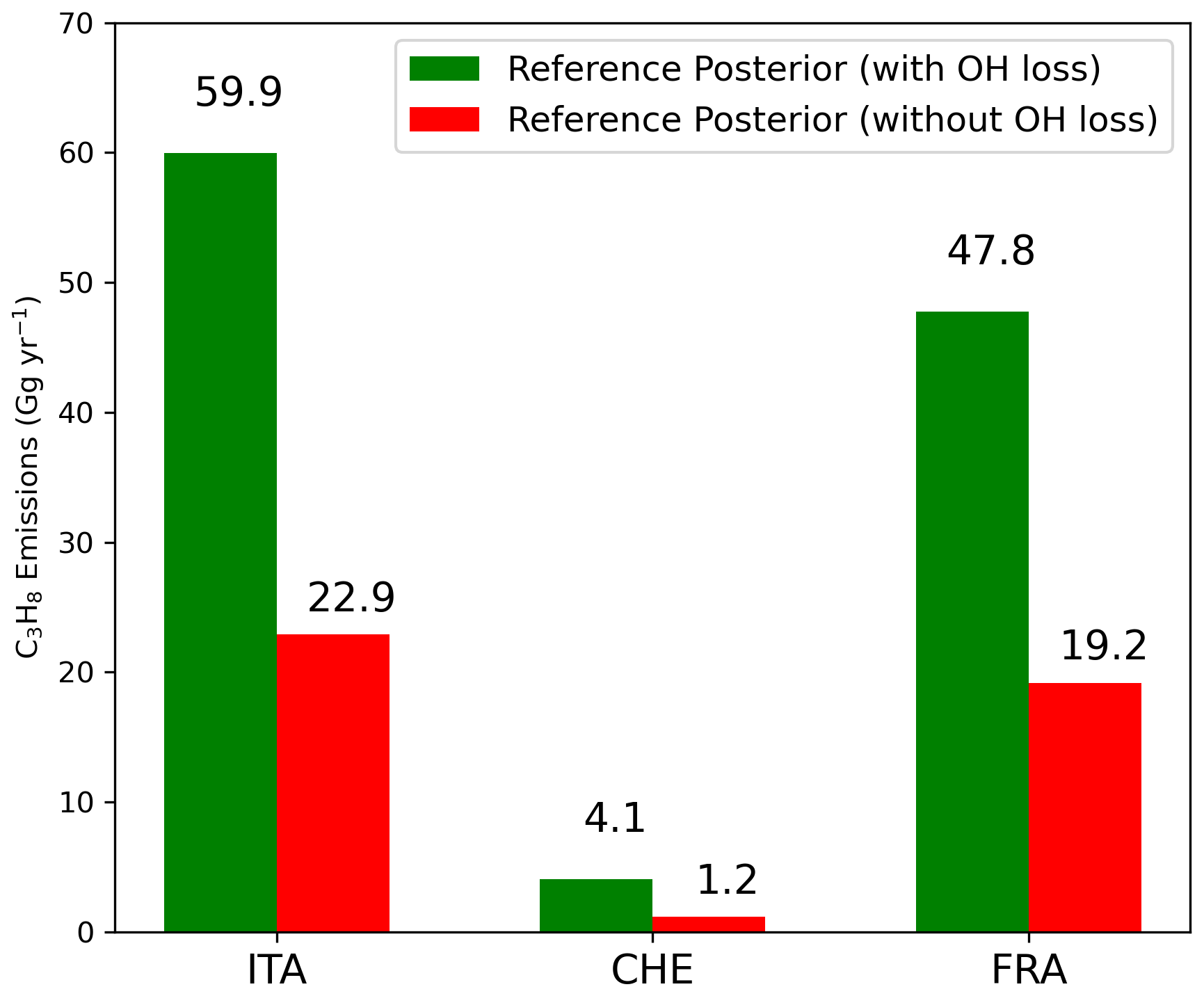
Figure E1 Comparison of posterior C₃H₈ emission estimates obtained from sensitivity test inversions using FLEXPART simulations that exclude OH chemical loss (red bars) versus the reference inversion that includes OH chemical loss (green bars).

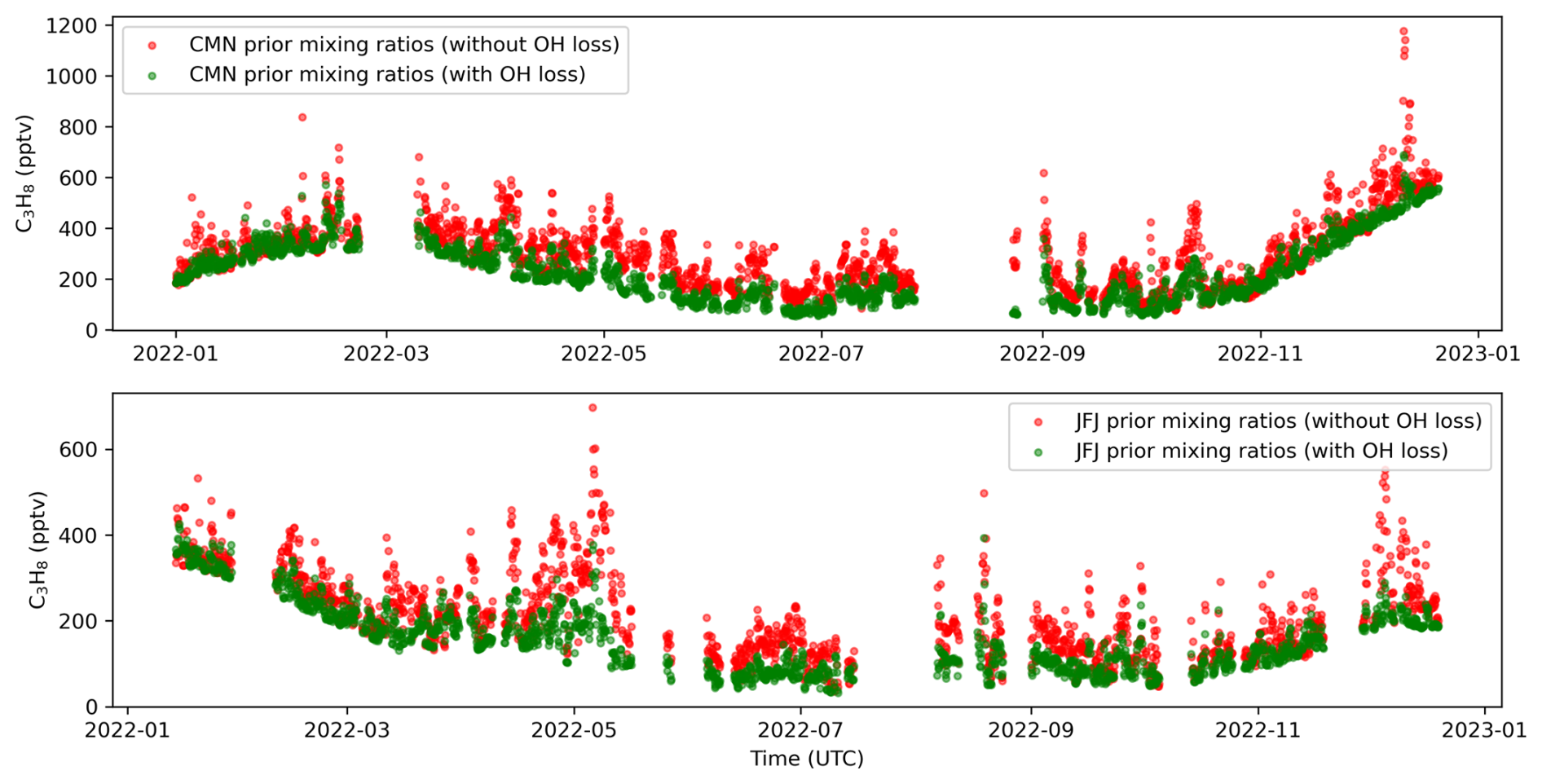
Figure E2 Time series of 3-hourly prior C₃H₈ mixing ratios simulated by FLEXPART at the CMN and JFJ sites, comparing simulations with (green dots) and without OH chemical loss (red dots).

Appendix F: Working standard statistics

Table F1 Working standard mixture calibration data.

^∗ Drifting tank.

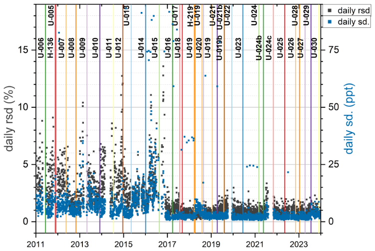
Figure F1 Instrumental reproducibility as the standard deviation of the daily working standard replicates, both as relative standard deviation (rsd %, in gray colour, on the left) and absolute (ppt, in blue colour, on the right) values. Vertical lines mark the date of the installation of a new working standard tank.