Tropical stratospheric upwelling as seen in observations of the tape recorder signal

Tropical upwelling constitutes the ascending branch of the global mean stratospheric circulation and governs the thermal and chemical properties of the tropical stratosphere. A lack of direct observations and a spread in upwelling structure across the modern reanalysis creates difficulties in determining variability and long-term changes of tropical upwelling. We have derived time series of effective vertical transport in the tropical lower and middle stratosphere from MLS and SWOOSH water vapour for 2005–2020 and 1995–2020. Our calculated upwelling is found to be in the range of 0.21–0.33 mm s⁻¹ for 73–28 hPa in very good agreement with reanalysis vertical velocities (ERA5, JRA-3Q, MERRA-2) and other observation-based estimates (ANCISTRUS).

We show that interannual variations of upwelling in the middle stratosphere are dominated by the QBO signal, which explains a large fraction of the upwelling anomalies. In the lower stratosphere, tropospheric modes of variability also play a role with the QBO and ENSO being equally important for explaining interannual variability. Individual peaks of strongly enhanced upwelling in the lower stratosphere in 2000/01 and 2011/12 cannot be explained by QBO or ENSO variability and coincide with known drops in water vapour and cold point temperatures. We use independent observational data to show that tropical upwelling is anticorrelated with long-lived stratospheric tracers such as ozone as expected, lending confidence to the derived values. A reduction in variability is observed for 2016–2020 in our calculated upwelling and observed ozone, which is consistent with the disruption to regular QBO variability over this period.

1 Introduction

The Brewer Dobson circulation (BDC) is the global wave-driven circulation of the stratosphere consisting of upwelling in the tropics and subsequent poleward transport and downwelling at higher latitudes (Brewer, 1949; Dobson, 1956; Butchart, 2014). The BDC is a dominant dynamical driver of the stratosphere and is important for the distribution of trace gases and therefore for stratospheric chemistry and radiative balance. In particular, the BDC contributes to both seasonal and decadal changes in stratospheric ozone (O₃) concentration, having far reaching influences spanning the annual cycle in the tropical lower stratosphere to variations in concentration in the polar regions (e.g., Randel et al., 2007; Tegtmeier et al., 2008; Weber et al., 2011; Fu et al., 2019). The entry value of water vapour (H₂O) into the stratosphere is highly dependent on the temperature of the tropical tropopause, which is modulated by tropical upwelling (Yulaeva et al., 1994). The relationship of the BDC with trace gases like ozone and water vapour is bidirectional, meaning that the transport of the BDC shapes distributions of the tracers and that radiative effects imposed by changes to trace gases have been shown to influence the strength of the BDC (e.g., Rind et al., 1998; Butchart and Scaife, 2001; Sigmond et al., 2004; Butchart et al., 2006).

Given the importance of the BDC for stratospheric tracer concentrations and subsequent chemical and thermal effects, great interest has been given to understanding its short- and long-term variability. Variations in tropical upwelling are primarily driven by variations in momentum deposition from large- and small-scale waves. In particular, planetary and synoptic-scale wave breaking in the extratropical and subtropical stratosphere is considered a primary driver of tropical upwelling (e.g., Randel et al., 2008; Ueyama and Wallace, 2010; Zhou et al., 2012). Furthermore, equatorial planetary waves deposit westerly momentum in the tropical upper troposphere which also plays a role for upwelling variations (e.g., Ryu and Lee, 2010; Garny et al., 2011).

The tropical branch of the BDC exhibits a seasonal cycle with strongest upwelling occurring for Northern Hemisphere (NH) winter and weakest for NH summer (Rosenlof, 1995). This pronounced seasonal signal is driven by stronger propagation and dissipation of extratropical planetary waves during the NH winter season. Interannual variability of the BDC is also driven by variations in wave activity which are, among other things, modulated by the quasi-biennial oscillation (QBO) and the El Niño Southern Oscillation (ENSO). Model studies suggest that the ENSO positive phase is associated with increased tropical upwelling, and vice versa for the negative phase (Sassi et al., 2004; Randel et al., 2009; Calvo et al., 2010). Similarly, observational data has been used to show that cool temperature anomalies resulting from the QBO easterly shear give increased tropical upwelling, and vice versa for the westerly shear phase (Niwano et al., 2003). The strength of the increased upwelling brought on by easterly QBO shear and positive ENSO is magnified if coinciding with the NH winter season, when upwelling is at its seasonal peak (Calvo et al., 2010; Neu et al., 2014).

With a magnitude on the order of 10⁻¹ mm s⁻¹, the vertical branch of the BDC cannot be directly measured. Instead, indirect estimates of upwelling are determined through the application of a framework like the transformed Eulerian mean (TEM; Andrews et al., 1987) approach that uses climate model output or reanalysis quantities (e.g. Butchart, 2014, and references therein; SPARC, 2022). The TEM equations are a mathematical representation of the advective component of the BDC, the so-called residual meridional circulation, which excludes the effects of wave-driven mixing on stratospheric composition. The lack of observations poorly constrains upwelling within reanalysis products. The residual vertical velocity derived as part of the TEM equations reveals differences in the structure of the circulation between the different reanalyses (Fujiwara et al., 2024). Consistently, the tropical upwelling mass fluxes in modern reanalyses show differences for basic climatological diagnostics such as structure, seasonality, and upwelling strength, the latter especially below 70 hPa (SPARC, 2022).

While the BDC can be analyzed directly from reanalyses or model output, observations provide only indirect estimates of the circulation. Most commonly, measurements of long-lived trace gases are used to infer characteristics and variability of the BDC (e.g., Mote et al., 1996; Niwano et al., 2003; Flury et al., 2013; von Clarmann and Grabowski, 2016; Glanville and Birner, 2017). As established by Mote et al. (1996), there exists a “tape recorder” signal in lower stratospheric tropical water vapour whereby the entry mixing ratio of water vapour is marked by the annual cycle of temperature at the tropical tropopause before being uplifted to higher levels. This creates a phase lag between the annual cycle of water vapour at different levels in the lower to middle stratosphere, which can be used to deduce the upward advection speed. This principle was applied by Niwano et al. (2003), where they calculated the ascent rate of anomalies in total water ([H₂O]+2[CH₄]) by correlating profiles staggered by altitude. The approach used in our study follows the method laid out by Schoeberl et al. (2008), and Flury et al. (2013), where this principle is applied by correlating time-lagged time series at different levels of the stratosphere to approximate the speed of tropical upwelling.

Here we estimate tropical upwelling from satellite measurements of water vapour made by the Microwave Limb Sounder (MLS) instrument, and from the Stratospheric Water and OzOne Satellite Homogenized dataset (SWOOSH). These and other data, along with our methods, are discussed in Sect. 2. Section 3.1 gives the first results, comparing the methods using the MLS and SWOOSH data, and using regression analysis to better understand the interannual variability caused by the QBO, ENSO, volcanic forcing, and the solar cycle. In Sect. 3.2, the upwelling calculated from MLS is compared to measurements of ozone from the Optical Spectrograph and Infrared Imager System (OSIRIS) satellite instrument. Here we discuss some features of variability that are common between the upwelling and ozone time series. In Sect. 3.3 the vertical component of the residual circulation calculated from the ERA5, JRA-3Q, and MERRA-2 reanalysis are compared to our calculated upwelling in terms of interannual variability and the seasonal cycle. We compare to another estimate of the tropical upwelling with ANCISTRUS data, to assess the similarities in interannual variability and in the climatological mean profile. Finally, we give conclusions in Sect. 4.

2 Data and Methods

2.1 Data

This study uses MLS version 5.1 level 3 daily water vapour, and monthly mean ozone and temperature. MLS was launched aboard the NASA Aura satellite in July 2004 and began making measurements in August 2004. The satellite operates in a 705 km sun-synchronous orbit and achieves 82° S to 82° N coverage on each orbit. About 14.5 orbits per day with 240 scans per orbit result in a total of about 3500 daily profile measurements, giving total coverage of the tropics approximately every 3 d (Waters et al., 2006). The water vapour data is valid between 316 and 0.001 hPa, and here we use data on the 100, 83, 68, 56, 46, 38, 32, 26, 22, and 18 hPa levels. The vertical resolution for the levels of interest ranges between about 3.5 to 3.8 km, degrading with increase in altitude, and the along track horizontal resolution is about 200 km. The accuracy of the measurements for this vertical range is reported as between 5 % and 8 % (Livesey et al., 2022).

The version 2.7 SWOOSH data used here is prepared on a 5 d temporal resolution interpolated to the Aura MLS vertical grid, and we use the “combinedh2oq” product. The SWOOSH water vapour data product is a composite of data from SAGE-II (v7, October 1984–August 2005), UARS MLS (v6, September 1991–April 1993), UARS HALOE (v19, October 1991–November 2005), SAGE-III/M3M (v4, February 2002–November 2005), ACE-FTS (v5.2, February 2004–present), Aura MLS (v5.1, August 2004–present), and SAGE III/ISS (v5.3, June 2017–present). Details of the SWOOSH data preparation are available in Davis et al. (2016). Despite the data being available from 1986, the early portion of the record is sampled too sparsely to be of use for this study, therefore, the SWOOSH data are taken from 1994 onward. The satellite instruments included in SWOOSH preceding Aura MLS lack the dense temporal and spatial coverage provided by Aura MLS, therefore while useful for extending the data record into the 1990s the lack of dense sampling necessitates averaging into a coarser temporal grid. The SWOOSH data require some preprocessing before use in the upwelling calculation because of the many gaps before 2005. To obtain a gap free time series, first the data is averaged in a zonal mean over 20° S to 20° N to incorporate as many observations as possible within the deep tropics. This is a wider zonal mean than we use for the MLS data (10° S to 10° N) and is done to obtain better statistics for the earlier period by including a greater number of observations in the mean. Noise from this zonal mean time series is smoothed with the application of a Savitzky-Golay filter (Savitzky and Golay, 1964), which also acts to interpolate the gaps to create a smooth signal. The filter uses linear least squares to fit order 3 polynomials to segments of the time series 21 data points long (105 d segments, with the data on a 5 d resolution). This step is necessary for the SWOOSH data in order to resolve the tape recorder signal for the early portion of the time series where the measurements are sparse and the data is noisy.

Level 2 version 7.3 ozone data is used from the OSIRIS satellite instrument. OSIRIS operates in a 600 km sun-synchronous orbit, making measurements of the limb from the upper troposphere to the lower mesosphere (Llewellyn et al., 2004). The vertical resolution of the instrument is between 1–2 km in the middle atmosphere (Murtagh et al., 2002), and we use data on the 27.5, 26.5, 24.5, 23.5, 22.5, and 21.5 km altitude levels. The version 7.3 data benefit from the drift correction applied in version 5.10, which removed the long-term drift beginning in 2012 that affected the limb-pointing of the instrument (Bourassa et al., 2018).

We compare residual vertical velocities from reanalyses with our vertical velocity estimates calculated from observations. For this purpose, we use the vertical component of the residual mean meridional circulation on pressure levels (${\stackrel{\mathrm{‾}}{\mathit{\omega }}}^{\ast }$) calculated from vertical velocity based on ERA5 (European Centre for Medium-range Weather Forecasts Reanalysis version 5; Hersbach et al., 2020), JRA-3Q (Japanese Reanalysis for Three Quarters of a Century; Kosaka et al., 2024), and MERRA-2 (Modern-Era Retrospective Analysis for Research and Applications version 2; Gelaro et al., 2017). The TEM zonal mean diagnostics of these reanalysis datasets, including the residual vertical velocities, are provided by Martineau (2022) and described in detail in Martineau et al. (2018). The TEM equation for ${\stackrel{\mathrm{‾}}{\mathit{\omega }}}^{\ast }$ is:

$$\begin{array}{}\text{(1)}& {\stackrel{\mathrm{‾}}{\mathit{\omega }}}^{\ast }=\stackrel{\mathrm{‾}}{\mathit{\omega }}+{\displaystyle \frac{\mathrm{1}}{a\cos \mathit{\varphi }}}{\displaystyle \frac{\partial }{\partial \mathit{\varphi }}}\left[{\displaystyle \frac{\stackrel{\mathrm{‾}}{v^{\prime }{\mathit{\theta }}^{\prime }}\cos \mathit{\varphi }}{\partial \stackrel{\mathrm{‾}}{\mathit{\theta }}/\partial p}}\right]\end{array}$$

Where $\stackrel{\mathrm{‾}}{\mathit{\omega }}$ is the zonal mean vertical velocity, a is the Earth's radius, ϕ is latitude, v^′ is the meridional wind anomaly, θ^′ is the potential temperature anomaly, and p is pressure. For more direct comparison with our estimates in units of mm s⁻¹, we convert the reanalysis vertical velocity from ${\stackrel{\mathrm{‾}}{\mathit{\omega }}}^{\ast }$ [Pa s⁻¹] to ${\stackrel{\mathrm{‾}}{w}}^{\ast }$ [mm s⁻¹].

The Analysis of the Circulation of the Stratosphere Using Spectroscopic Measurements (ANCISTRUS) is an inversion framework that derives effective meridional and vertical transport velocities from measured tracer fields by solving the continuity equation in a 2-D model (von Clarmann and Grabowski, 2016). These velocities are not equivalent to the Transformed Eulerian Mean (TEM) residual circulation and should not be interpreted in that framework. Instead, they represent the combined transport effect of advection and mixing required to reproduce the observed tracer distributions. Although the original formulation includes explicit mixing coefficients, the current implementation applies a regularization that suppresses the diagnosed mixing term. In any case, mixing effects are implicitly incorporated into the effective velocities (von Clarmann et al., 2021), similar to the resulting vertical velocities of the lag-correlation method. The goal of ANCISTRUS is to infer information about stratospheric transport strength in a way that avoids some of the biases and uncertainties inherent in age-of-air-based diagnostics. Here we use the L3 effective transport velocities from Kerzenmacher et al. (2025).

2.2 Methods

We calculate the vertical velocity by correlating 1 year long segments of the water vapour time series on two staggered vertical levels, where the time series on the upper level is lagged with respect to the lower level, following the method laid out by Schoeberl et al. (2008) and Flury et al. (2013). The staggered levels are taken to have a separation of about 4.5 km; the level pairs for the calculation are 100 and 46, 83 and 38, 68 and 32, 56 and 26, 46 and 22, and 38 and 18 hPa. These are wider separations compared to those used in the previous studies (Schoeberl et al., 2008; Flury et al., 2013). This choice of level spacing was made according to the vertical resolution of the MLS instrument such that the time series being correlated are independent in the averaging kernel, thus giving a more robust calculation for the wider compared to narrower level spacings. In sensitivity testing we found that using larger level spacing resulted in lower uncertainty in the calculated upwelling, and fewer unphysical features in the time series. The approximately 4.5 km level separation was chosen to minimize the uncertainties in the dataset arising from correlation curves peaking at very small lag lengths, the appearance of multiple peaks in the correlation curves, and broadness of the correlation maxima.

The vertical extent of the upwelling calculation is limited by the extent of the tape recorder signal. The tape recorder signal extends up to about 10 hPa, as it is attenuated with increasing height in the stratosphere as a result of mixing processes and oxidation of methane (Mote et al., 1996). Due to the attenuation the signal becomes less clear with altitude, therefore, here we are confined to the lower and middle stratosphere up to about 18 hPa, as above this level it is found that the signal is no longer sufficiently clear for the application of the time-lagged method.

To obtain units of mm s⁻¹ from the water vapour data which is natively given on pressure altitude vertical coordinates we convert the pressure altitude coordinates from hPa to m using climatological mean tropical altitude data. The correlation is calculated for a lag of zero to 360 d in 1 d increments, and the transit time between the levels is calculated from the lag corresponding to the maximum correlation. The value for maximum correlation is required to be greater than 0.6 to ensure that data that are not well correlated are not included in the time series. The value obtained for transit speed is assigned to the midpoint between the first day of the non-lagged time series, and the last day of the time series with the lag corresponding to the maximum correlation applied. Therefore, the speed assigned to any given day represents an average over approximately the preceding and following 6 months. This coarse time resolution smooths the variability on the seasonal time scale, leaving only interannual variations in the upwelling. To avoid anomalous results from the inclusion of the Hunga Tonga-Hunga Ha'apai eruption and aftereffects, we take data only to the end of 2021 for both MLS and SWOOSH giving calculated upwelling time series that end in 2020.

While using longer segments of the time series for performing the upwelling calculation allow for a more robust correlation calculation, Glanville and Birner (2017) demonstrated that it is also possible to perform the time-lagged correlation calculation taking 6 month long segments of the time series. This method allows for variability on the seasonal scale to be captured along with interannual variations. To observe some of this seasonal variability, in addition to the calculation based on the 12 month correlation method, here we also apply the same time-lagged correlation method as described above but use 6 month long segments of the water vapour time series and calculate correlations for lags between zero and 360 d. To avoid unrealistic results, the lag corresponding to the maximum correlation is required to be greater than 6 d, following Glanville and Birner (2017). Given a possible lag of between 7 and 360 d and the level widths used in the calculation, the method is capable of resolving speeds between approximately 0.15 and 7.98 mm s⁻¹. We find in general that while there is good agreement between the 12 and 6 month methods, there is a higher level of uncertainty in the estimates from the 6 month method. Therefore, we use the results from the 12 month method everywhere in this paper where we are interested in interannual rather than seasonal variability.

The factors contributing to uncertainty in upwelling calculated with lagged correlations of the water vapour tape recorder include measurement uncertainty and uncertainty introduced by the method. To estimate the uncertainty in the calculated upwelling, we construct bounds on the upwelling estimates based on confidence intervals of the correlation coefficients for the lagged correlation of segments of the water vapour time series. A 95 % confidence interval is determined for each correlation coefficient, and on either side of the peak of the correlation curve the first correlation value that is statistically different from the maximum is chosen to determine the bound on the upwelling speed. Sensitivity testing found that there was negligible difference in the amount of uncertainty if the confidence level was chosen as 90 %, 95 %, or 99 %.

The time lag-correlation method is a calculation of the total transport between stratospheric levels, including the effect of mixing in addition to transport by the BDC. This effect was investigated by Mote et al. (1998), who found that their estimate of the ascent rate of the tape recorder signal was slightly stronger than the true advection velocity and attributed this difference to vertical diffusion. They found that the rate of diffusion was positive (indicating net upward mixing) for the region between 18 and 31 km. Therefore, the effect of vertical mixing should in general be to cause homogenization of the tape recorder signal at subsequent levels, with the mixing acting in the upward direction, causing a reduction in the time-lag of the signals and leading to a faster calculated upwelling. Further discussion of this effect and the agreement between the tape-recorder derived velocity and the residual circulation is given in Sect. 3.3.

3 Results

3.1 Upwelling calculated from MLS and SWOOSH water vapour

Time series of tropical upwelling were calculated using the 12 month time-lagged correlation method for October 2005 to December 2020 from MLS water vapour, and for January 1995 to December 2020 from SWOOSH water vapour. The data for this calculation were taken from the deep tropics; a zonal mean over 10° S to 10° N for MLS and 20° S to 20° N for SWOOSH. The climatological mean profile is shown in Fig. 1. The data for the profile were plotted at the midpoint of the layers used in calculating the upwelling, and due to the level spacing there is overlap between the layers used in the calculation. Therefore, although the profile is gridded on a 1 km grid, it should be held in mind that the upwelling is calculated over layers about 4.5 km deep. There are only small differences between the MLS and SWOOSH profiles, as expected since SWOOSH includes the MLS data in the merged data. The values for upwelling span between 0.21–0.33 mm s⁻¹, minimizing around 50 hPa and maximizing at the boundaries of our profile. These values and profile shape are in line with other similar estimates as found in Mote et al. (1998), and Schoeberl et al. (2008).

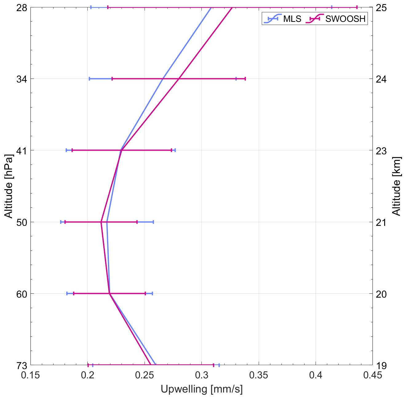
Figure 1 Profile of climatological mean tropical upwelling calculated from MLS and SWOOSH water vapour in the lower stratosphere. Horizontal bars give the uncertainty range derived as the 2σ standard deviation of the monthly time series.

The profiles in Fig. 1 show upwelling calculated from the correlations of 12 month long segments of the water vapour time series, giving a smoothing of about a year. The shape and values of the profiles from the method correlating 6 month long segments of the time series (not shown) are largely indiscernible from that shown here. Therefore, variability in the time series that is lost in the smoothing that is implicit in the application of the time-lagged correlation method is not found to contribute significantly to the climatological upwelling profile.

The interannual variability in upwelling can be seen in the time series of Fig. 2. The shading indicates uncertainty introduced by the lag-correlation method, calculated using the 95 % confidence interval on the correlation coefficients. Here again there is good agreement between MLS and SWOOSH (correlation coefficients ranging between 0.89 and 0.97 for the six levels investigated here), as expected. There are some gaps in the portion of the SWOOSH upwelling time series before 2005 which are a result of reduced vertical coherence for these earlier years. The effect of this is to give smaller correlations between the levels. In some cases the maximum lagged correlation falls below the threshold value of 0.6 used here, meaning that no value is assigned for that day's calculation and creating a gap in the time series.

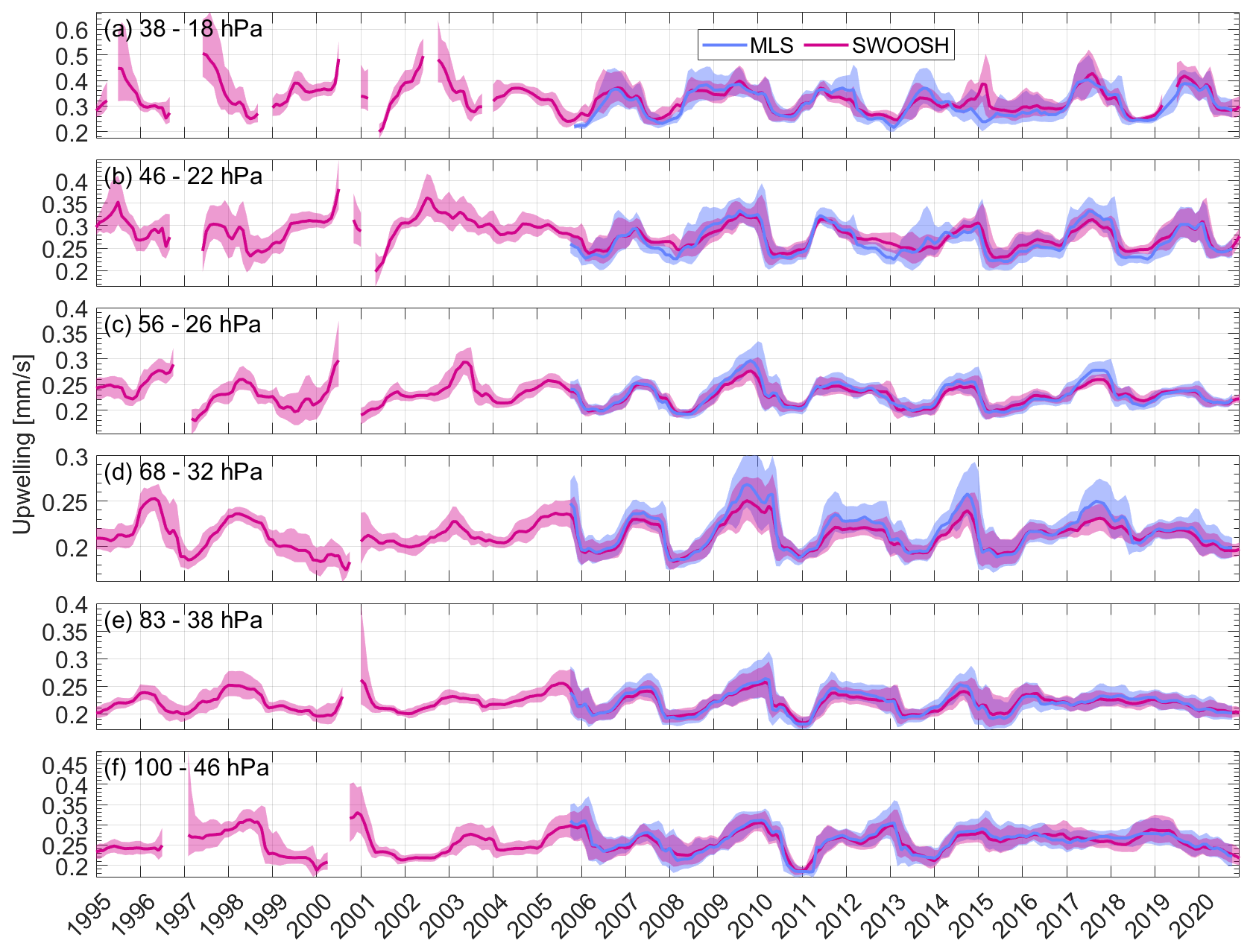
Figure 2 Time series of upwelling calculated from 12 month correlations of MLS and SWOOSH water vapour for (a) 38–18 hPa, (b) 46–22 hPa, (c) 56–26 hPa, (d) 68–32 hPa, (e) 83–38 hPa, and (f) 100–46 hPa. Shading indicates time-dependent error bars of the upwelling estimates calculated from the 95 % confidence interval of the correlation coefficients.

A multilinear regression analysis was used to aid in the understanding of the factors driving the variability in upwelling. Variability due to the QBO, ENSO, solar forcing, and volcanic aerosol forcing was modelled through the use of the first two QBO empirical orthogonal functions calculated from Singapore zonal wind soundings (Naujokat, 1986; Wallace et al., 1993), the multi-variate ENSO index (MEI; https://psl.noaa.gov/enso/mei/, last access: 5 March 2026), f10.7 solar flux (https://psl.noaa.gov/data/correlation/solar.data, last access: 5 March 2026), and GLoSSAC (Global Satellite-based Stratospheric Aerosol Climatology) stratospheric aerosol optical depth (SAOD; Kovilakam et al., 2020). The upwelling was lagged two months behind the MEI in the regression model, and the other three parameters were applied with no lag. A lag of two months for the MEI was determined to produce the best results for minimizing the residuals across the six different levels. In sensitivity testing, it was found that the choice of lag did not have a significant impact on the results presented here, and therefore the fixed value was used. This analysis model is limited to capturing linear effects, and therefore possible non-linear effects that could be influencing the upwelling time series are not considered here.

The regression analysis was performed for upwelling calculated using the 12 month time-lagged correlation method from both MLS and SWOOSH. Figure 3 shows examples of the regression fit and residuals for SWOOSH at 100–46 hPa in panels a and b, and MLS at 68–32 hPa in panels c and d (note that the vertical scales are different in each panel of Fig. 3), these will be discussed in detail later in this section. The regression fits and residuals for both instruments at all six levels are shown in Appendix A (Fig. A1). The residuals are quite small but are not randomly distributed, indicating that there is some cyclic signal impacting the upwelling that is not captured in the regression. The adjusted R² ($R_{\text{adj}}^{\mathrm{2}}$) values at each altitude level are shown in Fig. 4. The R² metric explains the percentage of variability in upwelling that is explained by the regressors, and the adjusted R² accounts for the number of regressors in the model. The significance of the $R_{\text{adj}}^{\mathrm{2}}$ were evaluated with a two-tailed p-test at 95 % confidence after adjusting the degrees of freedom to correct for autocorrelation of the residuals (e.g. Santer et al., 2000). To assess the strength of the contribution from each parameter individually, $R_{\text{adj}}^{\mathrm{2}}$ are given for regression with each of the QBO, ENSO, solar forcing, and volcanic forcing regressed alone, as well as for the full model with all four parameters included. The values for $R_{\text{adj}}^{\mathrm{2}}$ range from 0.59 to 0.72 for MLS, and from 0.41 to 0.57 for SWOOSH for the full regression model, demonstrating that a large portion of the variability in upwelling is described by the QBO, ENSO, volcanic forcing, and solar cycle together. The diminished $R_{\text{adj}}^{\mathrm{2}}$ values for SWOOSH compared to MLS were assessed with respect to the differences in the data sets in time and space and are discussed further in this section.

To assess the factors contributing to the smaller $R_{\text{adj}}^{\mathrm{2}}$ values found for SWOOSH, the regression model was applied to SWOOSH for the MLS period (2005–2020), and to MLS for a mean over 18° S to 18° N to have a more direct comparison in time and space. When regressing the SWOOSH data over the shorter time period, the $R_{\text{adj}}^{\mathrm{2}}$ values improved to span between 0.48 and 0.64, whereas for MLS the impact of regressing over a broader zonal mean was a reduction in the $R_{\text{adj}}^{\mathrm{2}}$ values to be between 0.46 and 0.64. The improvement in the $R_{\text{adj}}^{\mathrm{2}}$ for SWOOSH when taking the regression over the MLS portion of the time series indicates that there is some uncertainty being added to the time series from the earlier data which is noisier and more sparsely sampled than MLS. This is especially impactful for the levels above 68–32 hPa, where the tape recorder signal becomes less cohesive, giving higher uncertainty and larger gaps in the upwelling time series. This reflects how the uncertainty prior to the introduction of MLS to the SWOOSH data is higher than for the MLS period as a result of the less densely sampled data and should therefore be interpreted with more caution. The reduction in $R_{\text{adj}}^{\mathrm{2}}$ for MLS when calculating the upwelling over a broader zonal mean indicates that the influence of the regressors drops off quickly with distance from the tropics.

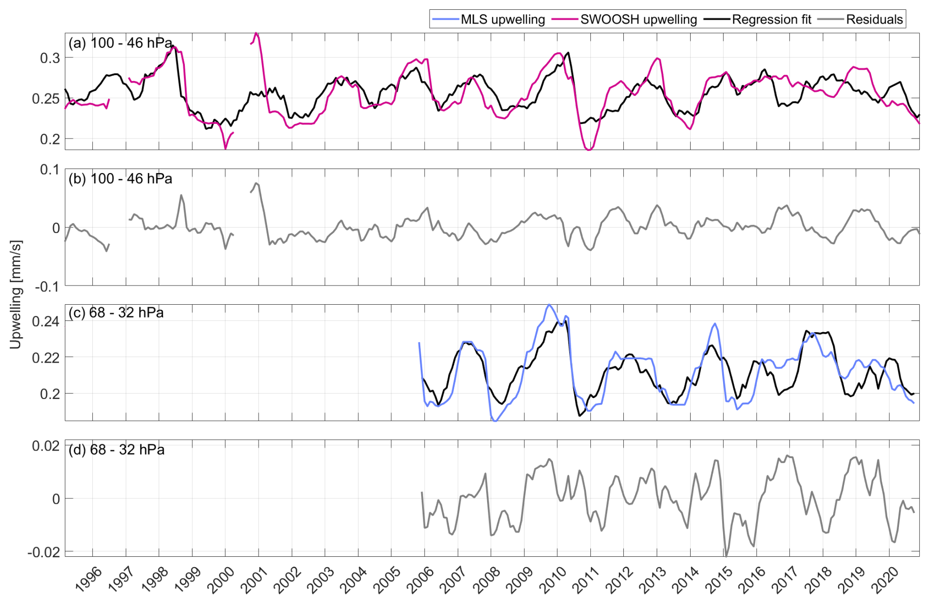
Figure 3 Time series of regression fits and residuals for (a, b) regression of 100–46 hPa SWOOSH upwelling, and (c, d) regression of 68–32 hPa MLS upwelling. Note the different vertical scaling for each panel. Uncertainty shading is omitted here to simplify the figure.

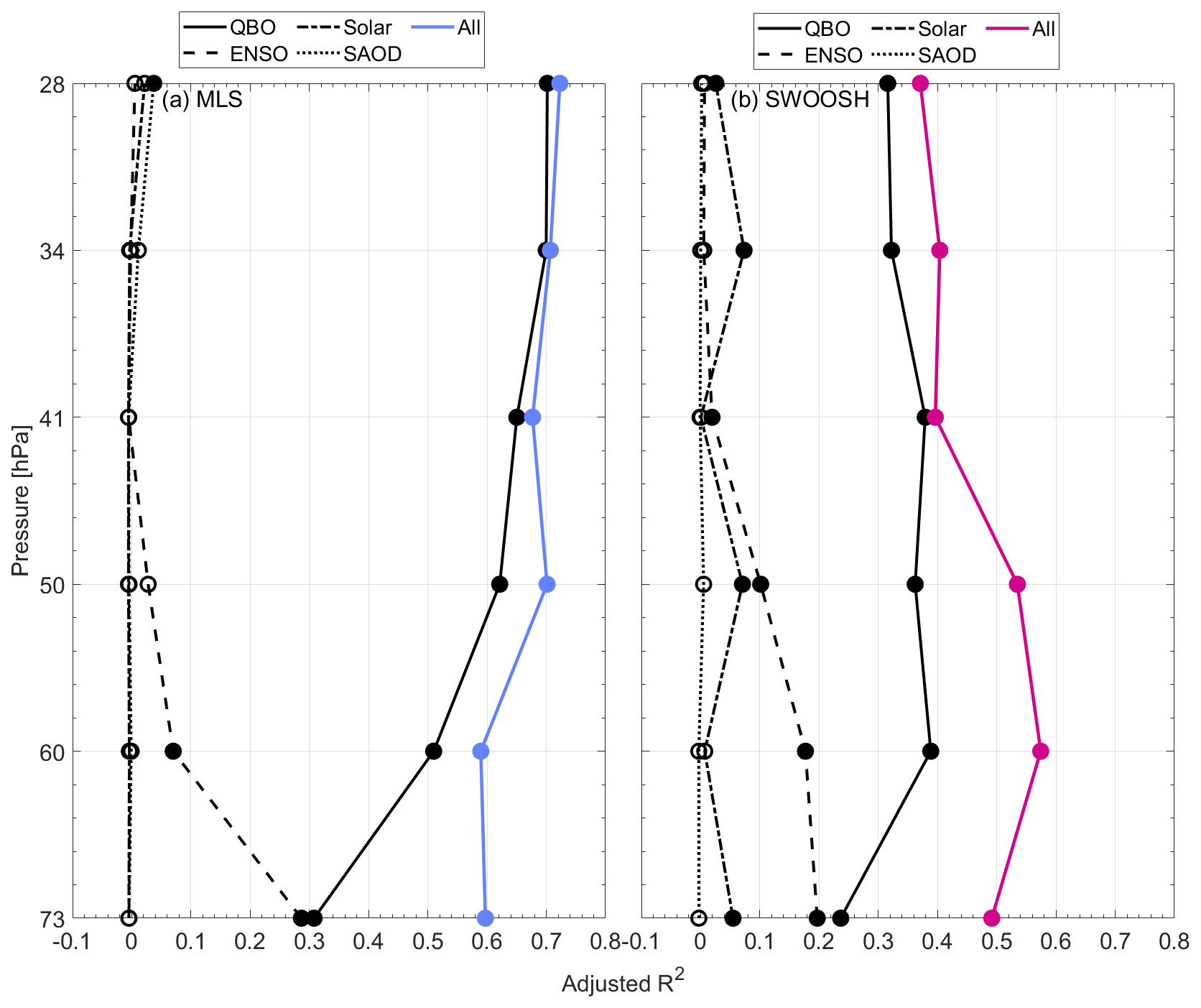
Figure 4 Profile of regression model adjusted R² for (a) MLS method upwelling and (b) SWOOSH method upwelling. Filled and unfilled circles represent significance and insignificance at the 95 % level, respectively.

The example regression fits in Fig. 3 highlight some of the interesting features of variability visible in the time series of Fig. 2. In Fig. 3a, there is a spike in lower stratospheric upwelling apparent around the year 2001. This spike represents not only the overall maximum upwelling over the full 26 year long record but is also special in a sense that it cannot be explained by a linear combination of QBO or ENSO variability in contrast to nearly all other temporal maxima. The enhanced tropical upwelling in late 2000/early 2001 coincides with anomalous low water vapour and cold point temperatures at the same time (Randel et al., 2006). On the contrary to TTL temperature and water vapour observations which experience a step-like decrease starting in 2001, we find only a temporary peak in upwelling in 2001 and a decrease back to regular values soon after. The step like change in water vapour has been shown to be partially consistent with changes in EP flux divergence from reanalysis (Randel et al., 2006). The divergence of the upwelling response in 2001 from previous observations could be related to the coarse vertical resolution for these upwelling estimates, or a result of the higher uncertainty for the pre-MLS portion of the time series potentially introducing artificial features into the calculated upwelling. Similar to the 2001 signal, there is a strong decrease in upwelling from mid-2010 to mid-2011, which can be only partially explained by the QBO and ENSO driven regression terms. This decrease in upwelling is consistent with an increase in stratospheric water vapour in 2011 (Dessler et al., 2013; Urban et al., 2014).

The time series of Fig. 3c demonstrates some variability that is driven by our regressed parameters. The regular quasi-biennial cycle in the upwelling is interrupted around 2015, leading to interannual variability on an anomalous timescale for the subsequent period of the time series. Correspondingly, the variability of the SWOOSH time series in Fig. 3a is greatly diminished following 2015, a feature that is mirrored to a large extent in the regression fit. These anomalous attributes of the time series following 2015 can be identified in the time series for Fig. 2d–f and are thought to be related to the QBO disruptions in 2015/16 and 2019/20. This point will be discussed further in Sect. 3.2.

The profiles of $R_{\text{adj}}^{\mathrm{2}}$ for each regression parameter in Fig. 4 demonstrate the strength of each of the QBO, ENSO, solar forcing, and volcanic forcing individually on upwelling variability. The shape of the profile and the relative contribution from each parameter differ slightly between MLS and SWOOSH, however, for both data sets the QBO is found to have an overwhelmingly dominant influence above the lowest level. At the bottom of the profile, the QBO and ENSO terms contribute a similar amount to the explained variability before the $R_{\text{adj}}^{\mathrm{2}}$ value for ENSO decreases sharply with altitude and becomes insignificant around the middle of the profile. These results for the contribution of the QBO and ENSO to the variability of tropical upwelling agree well with the results of Abalos et al. (2015), which show that the variability due to ENSO peaks in the lower stratosphere, and the variability due to the QBO increases with height up to about 20 hPa.

Some of the dissimilarities in the MLS and SWOOSH profiles appear in the variability explained by the QBO; for MLS the $R_{\text{adj}}^{\mathrm{2}}$ increases with altitude to the top of the profile, whereas for SWOOSH it begins to decrease above 41 hPa. This could be a result of the uncertainty introduced through the sparsely sampled data in the earlier portion of the time series, and higher uncertainty in the early portion of the time series in the levels above 68–32 hPa, as discussed above.

The last dissimilarity is found in the $R_{\text{adj}}^{\mathrm{2}}$ for the solar forcing. For MLS it is insignificant at all levels, whereas SWOOSH finds a small (around 0.05 to 0.1) but significant $R_{\text{adj}}^{\mathrm{2}}$ for the solar forcing at all levels other than 41 hPa. This can possibly be attributed to the fact that the SWOOSH time series is longer and therefore captures more variability due to the 11 year solar cycle. However, this could also be due to multi-decadal variability present in the longer time series such as found for water vapour (Tao et al., 2023), which is not necessarily resulting from the solar signal. A longer time series encompassing more solar cycles would allow for a more conclusive categorization of the signal in variability.

3.2 Upwelling and ozone

The amplitude and timing of the seasonal cycle in ozone in the tropical lower stratosphere is impacted by both in-mixing from the midlatitudes, and tropical upwelling (e.g., Abalos et al., 2013; Stolarski et al., 2014). The profile of ozone in the tropical upper troposphere and lower stratosphere has a positive gradient from the low tropospheric values to the maximum values of the stratospheric ozone layer, and in-mixing transports ozone rich air from higher latitudes to the tropics. Therefore, in-mixing impacts the vertical gradient of ozone in the tropics, and increased upwelling uplifts ozone poor air leading to an anticorrelation between ozone and upwelling in the tropics which is complicated by the process of in-mixing (Abalos et al., 2012; Abalos et al., 2013; Stolarski et al., 2014). The alignment of phasing of the tropical upwelling and midlatitude in-mixing can influence the seasonal cycle of ozone in the tropical lower stratosphere, and leads to hemispheric asymmetries (Stolarski et al., 2014).

To verify that our upwelling estimates follow this expected relationship, Fig. 5 shows time series of upwelling calculated from MLS using the 12 month lag-correlation method along with zonal mean tropical ozone (10° S to 10° N) measured by the OSIRIS instrument. Here the upwelling and ozone are plotted as anomaly time series, with the seasonal cycle removed from each monthly mean value. The ozone time series were smoothed with a 13 month running mean to match the temporal resolution of the calculated upwelling. Given that upwelling transports ozone anomalies from below to any given level, we correlate upwelling in a given layer with the ozone at the top of this layer. In particular, the altitude level for the ozone time series was chosen to best match with the upper level of the corresponding calculated upwelling. As a sensitivity test, we have also instead taken ozone as a mean over the upwelling layer and find lower correlations between the ozone and upwelling over the respective layer when compared to taking ozone at the top of the layer, as shown in Appendix B (Fig. B1). A similar comparison is done for HCl in Appendix B (Fig. B2).

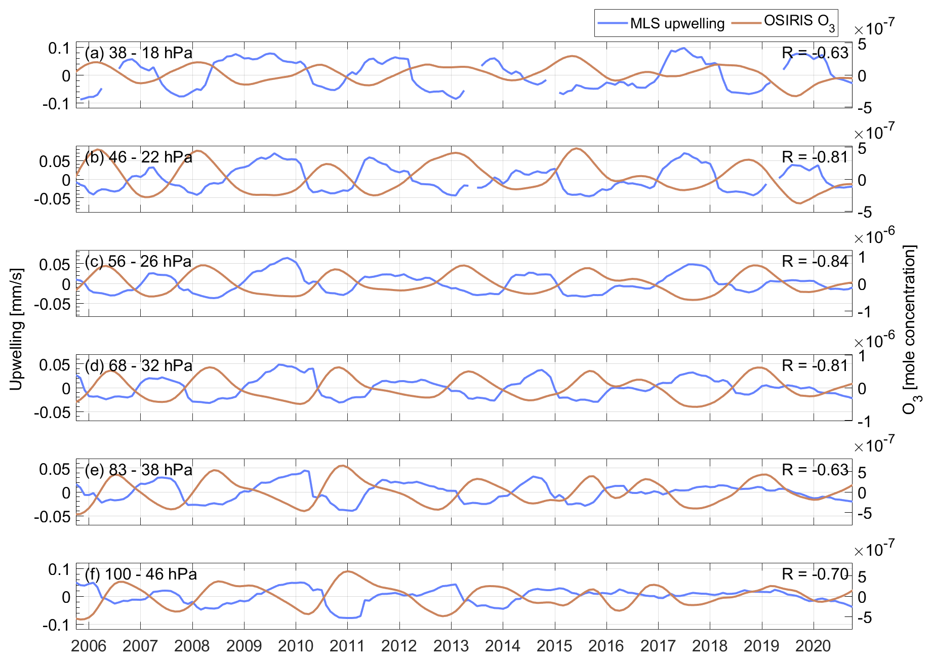
Figure 5 Time series of upwelling anomalies from MLS plotted along with O₃ anomalies from OSIRIS for (a) MLS between 38–18 hPa and OSIRIS O₃ at 27.5 km (about 18 hPa); (b) MLS between 46–22 hPa and OSIRIS O₃ at 26.5 km (about 20 hPa); (c) MLS between 56–26 hPa and OSIRIS O₃ at 25.5 km (about 27 hPa); (d) MLS between 68–32 hPa and OSIRIS O₃ at 23.5 km (about 33 hPa); (e) MLS between 83–38 hPa and OSIRIS O₃ at 22.5 km (about 37 hPa); and (f) MLS between 100–46 hPa and OSIRIS O₃ at 21.5 km (about 45 hPa). Uncertainty shading is omitted here to simplify the figure.

We find strong anticorrelations between the OSIRIS ozone and MLS upwelling of −0.63, −0.81, −0.84, −0.81, −0.63, and −0.70 for panels a–f of Fig. 5, respectively. We do not show these time series for the SWOOSH upwelling or MLS ozone for brevity but find similar correlations in the range of −0.70 to −0.84 for MLS ozone with MLS upwelling, −0.60 to −0.75 for OSIRIS ozone with SWOOSH upwelling, and −0.61 to −0.81 for MLS ozone with SWOOSH upwelling. These strong anticorrelations demonstrate that the variability in our upwelling estimates is closely matched to the variability in ozone, as expected.

The agreement between our calculated upwelling and measured ozone and HCl extends to the reduced variability in the time series following about 2015 at the lowest levels (Fig. 5e and f) and demonstrates that this feature is not simply anomalously produced by the upwelling calculation method. The variance in MLS-derived upwelling and OSIRIS ozone decreases between the two periods (October 2005–December 2015 and January 2016–December 2020) by 71 % and 55 %, respectively, for 100–46 hPa, and by 80 % and 45 %, respectively, for 83–38 hPa. This event in the time series coincides with the QBO disruptions in 2015/16 and 2019/20 (e.g. Osprey et al., 2016; Anstey et al., 2021). These events saw the first case of a deviation from the consistent quasi-biennial cycling between easterly and westerly winds that has been observed in the stratosphere by radiosondes since the 1950s. Previous studies have shown that the impact of the QBO disruption on tropical circulation produced a negative anomaly in tropical ozone (Diallo et al., 2018, 2022).

To investigate the role of the QBO disruption on the observed reduction in variability for upwelling and ozone more closely, a time series of detrended temperature anomalies was produced from MLS temperatures. The temperature response to changes in upwelling has been shown to be a combination of a dynamic response due to adiabatic effects and a radiative response due to changes in ozone concentrations (e.g., Randel et al., 2021). As both upwelling and ozone show a reduced variability after 2015, the same can be expected for temperature. A detrended, zonal mean (10° S to 10° N) temperature time series averaged over the pressure levels for the upwelling calculation is shown in Fig. 6. Here, similar to what is seen for upwelling and ozone, the temperature anomalies in the lower stratosphere have a reduced variability following 2015. The reduction in variance from the period up to December 2015 to the period from January 2016 to December 2020 is 31 % for the averaged layer from 100–46 hPa, and 44 % for the averaged layer from 83–38 hPa. The similarities in the variability changes occurring around the QBO disruptions in each of the upwelling, ozone, and temperature signals demonstrates the influence of the disrupted QBO on the overall variability of the tropical lower stratosphere.

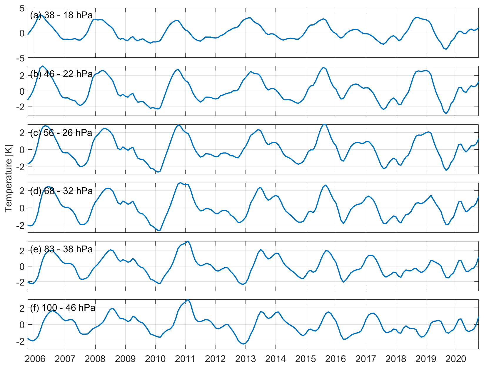
Figure 6 Detrended MLS temperature anomaly time series for the averaged levels (a) 38–18 hPa, (b) 46–22 hPa, (c) 56–26 hPa, (d) 68–32 hPa, (e) 83–38 hPa, and (f) 100–46 hPa.

3.3 Upwelling and reanalysis vertical residual circulation

Here we evaluate the vertical component of the residual circulation from ERA5, JRA-3Q, and MERRA-2 reanalysis by comparing the reanalyses to our upwelling estimates. The TEM calculation for the vertical residual circulation is an estimate of the vertical transport by the BDC, without any impact from mixing, whereas our estimates are of the total transport. The tracer-based method introduces unavoidable deviations from the true residual transport through uncertainties in the measurements, impacts from mixing, and uncertainty due to the calculation method. Therefore, the success of the lag-correlation estimate in representing the true residual circulation is dependent on the size of the uncertainties in the calculated upwelling and on the strength of diffusion and dilution of the water vapour signal.

Previous studies have assessed the similarities between the tape-recorder derived vertical transport speed and the residual transport in models and reanalyses. Mote et al. (1998) compared the advection speed of the tape recorder signal (2[CH₄]+[H₂O]) from the HALOE (Halogen Occultation Experiment) instrument to an estimate of the residual circulation calculated with UARS (Upper Atmosphere Research Satellite) data within the TEM framework, and found very strong agreement in a tropical mean profile between 19 and 24 km. Schoeberl et al. (2008) calculated the vertical transport speed from HALOE and MLS water vapour, and compared to the speed calculated from the tape recorder signal in the GEOS-CCM (Goddard Earth Observing System chemistry-climate model). They found good agreement between the residual vertical velocity and the water vapour tape recorder derived vertical velocity in the GEOS-CCM for the region between 19 and 26 km, albeit with the tape recorder derived velocity being slightly faster than the residual vertical velocity. From the estimates of vertical velocity calculated from observations of water vapour compared to the GEOS-CCM results, they concluded that the tape recorder correlation method gives a reasonable estimate of the residual circulation which tends toward giving a slight overestimate. In the 5th SPARC (Stratospheric Processes and their Role in Climate) Report on the Evaluation of Chemistry Climate Models (Eyring et al., 2010), they use the age gradient as another tracer derived metric for tropical upwelling speed in addition to the tape-recorder derived vertical velocity. They demonstrate that in cases where the model age gradient and tape recorder derived vertical velocities agree with each other, the transport-derived vertical velocities in the model agree with observational estimates, indicating a strong role for the tracer-dependent terms.

In all, these previous studies have shown that the water vapour tape recorder lag correlation gives a good approximation to the residual circulation in the real atmosphere, with deviations from the residual circulation tending to appear as an overestimate. The ability of the tape recorder lag correlation method to produce reasonable transport speeds from model or reanalysis water vapour is dependent on the particulars of the speed of the transport circulation within the model framework. It has been demonstrated that there is an incoherence between the water vapour tape recorder and vertical residual velocity in reanalysis, likely due to enhanced vertical dispersion of water vapour due to data assimilation (Glanville and Birner, 2017; Linz et al., 2019). This produces an effective vertical speed of the reanalysis tape recorder which is multiple times too large compared to the observational estimates as calculated from the tape recorder lag correlation from satellite observations. The 12 month lag correlation method applied to the ERA5 daily water vapour produced speeds that were twice as large as the MLS estimate in the climatological mean profile (not shown here).

From the results of the previous studies discussed above, we expect our observational estimates of vertical velocity to be a good approximation of the residual circulation, however potentially giving a slight overestimate of the true speed. This effect is expected to be especially important for boreal summer when the circulation is at its annual minimum and therefore mixing has a stronger impact on total transport (Glanville and Birner, 2017; Poshyvailo et al., 2018). The residual circulation quantities calculated from the reanalyses are given as zonal mean values on a 2.5° latitude grid and on the 100, 70, 50, 30, 20, and 10 hPa pressure levels. The vertical component is given in pressure-coordinate units of Pa s⁻¹. To better match our calculations to the reanalysis values, we convert the reanalysis to units of mm s⁻¹ and average the reanalyses over consecutive pressure levels to correspond to the vertical resolution of our estimates.

Figure 7 shows a climatological mean profile of our upwelling estimates calculated from MLS water vapour along with the vertical component of the residual circulation from reanalysis for the same time period as the MLS estimate. The SWOOSH estimate was omitted here, as from Fig. 1 the SWOOSH profile is very similar to MLS. We find good agreement between all profiles in terms of absolute value. In addition to agreement of the absolute values, our estimates follow the same profile shape as the reanalyses, albeit with a stronger curve to the profile. The variability in the full reanalyses upwelling time series, represented by the 2 standard deviation error bars in Fig. 7, are up to about three times larger than those for the MLS upwelling. This is a reflection of the smaller amplitude of the seasonal cycle found for the MLS (and SWOOSH) calculated upwelling, which can potentially be attributed to the effect of mixing on the calculated transport. While the mixing in general should cause our estimates of upwelling to be stronger than the true value, the seasonal cycle in mixing can act to damp this effect for certain seasons, such that our seasonal mean is in general stronger than the reanalysis for NH summer, but comparable for NH winter, as seen in Figs. 8 and 9b, d, f, h, j, and l. This results in a flatter seasonal amplitude for the calculated upwelling, and a lower variability when compared to the reanalyses.

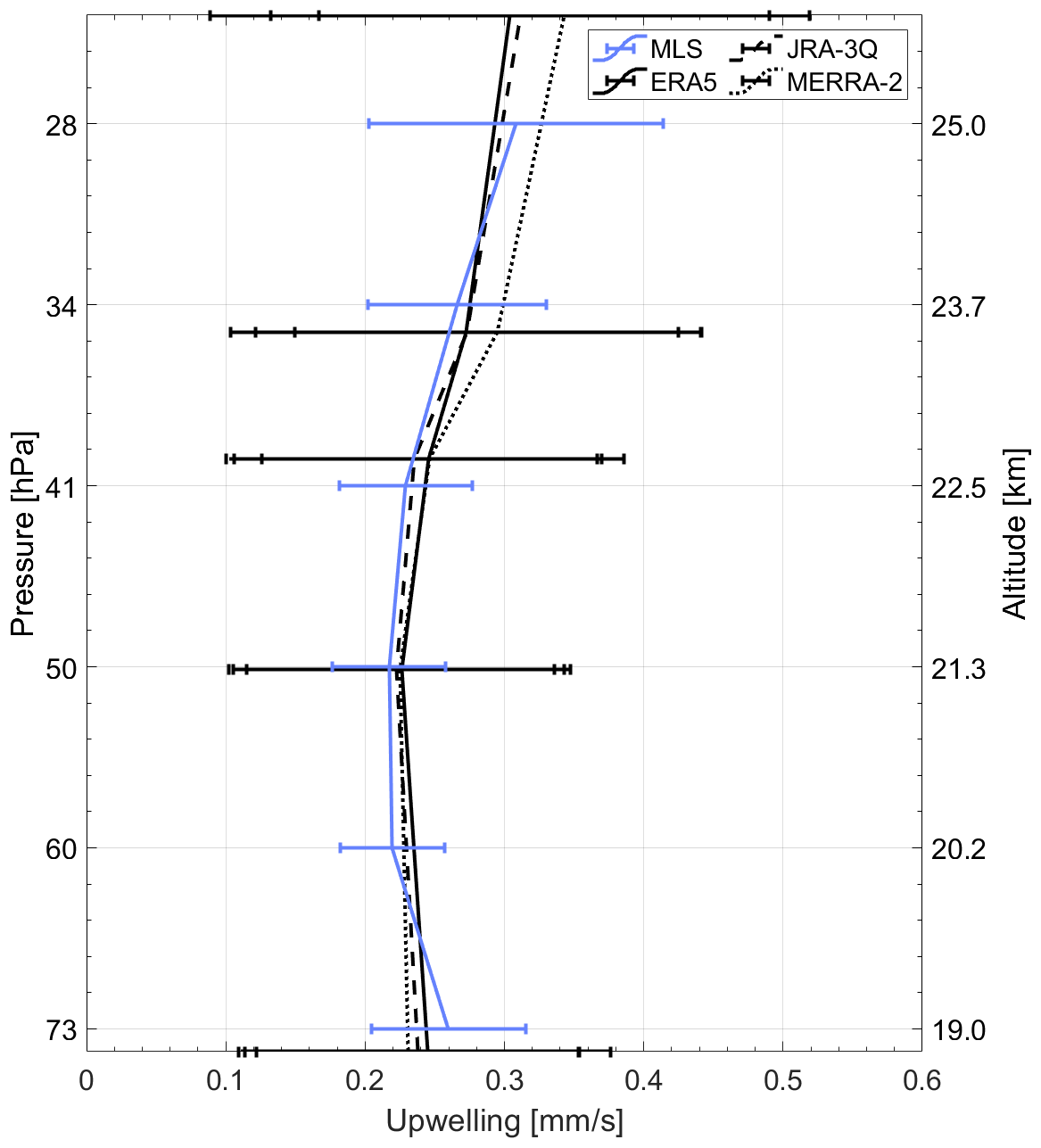
Figure 7 Climatological mean profile of upwelling from the MLS 12 month lagged correlation method and reanalysis vertical residual velocities. Horizontal bars give the uncertainty range derived as the 2σ standard deviation of the monthly time series.

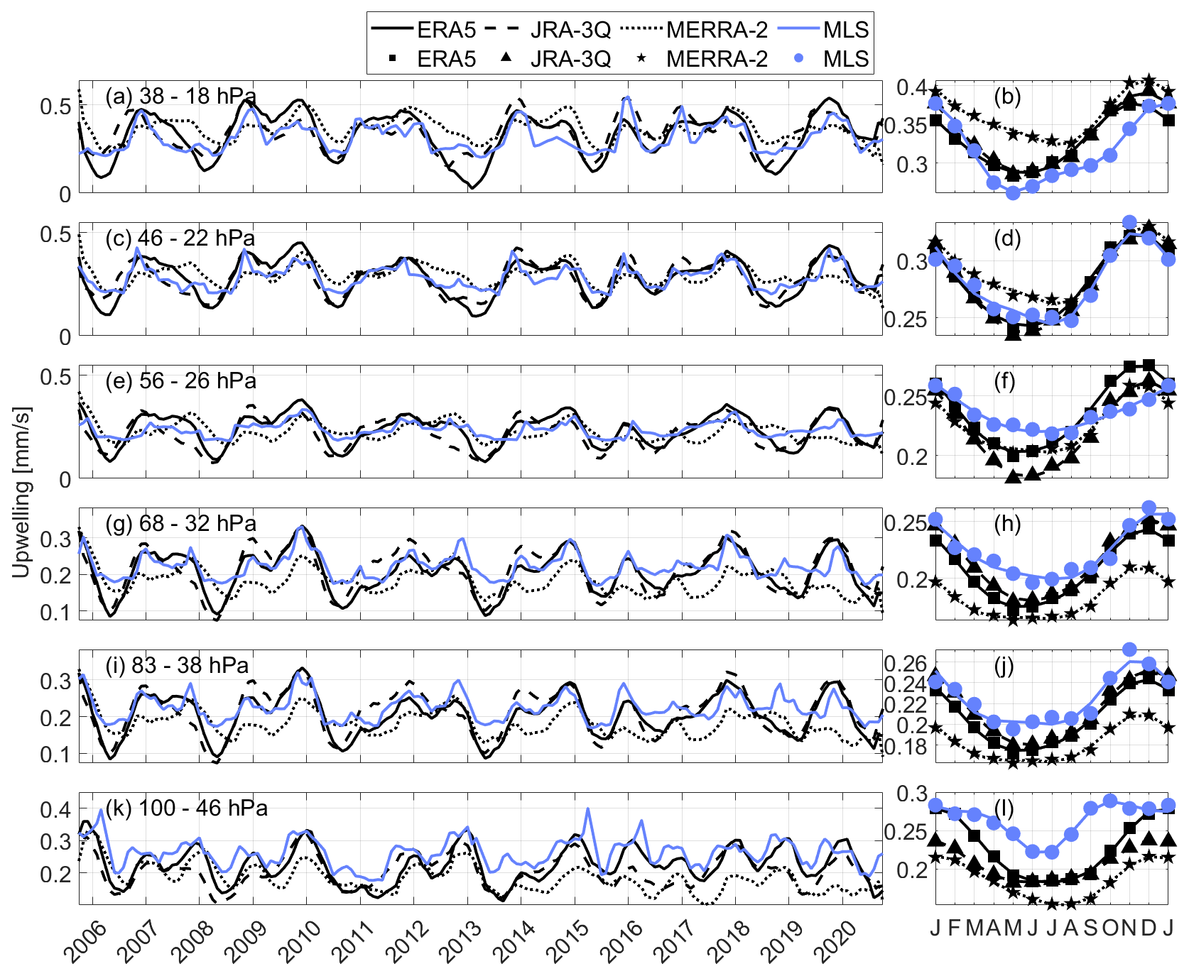
Figure 8 Tropical upwelling time series and corresponding seasonal cycle for upwelling calculated from MLS and the vertical component of the residual circulation from ERA5, JRA-3Q, and MERRA-2, for (a, b) 38–18 hPa, (c, d) 46–22 hPa, (e, f) 56–26 hPa, (g, h) 68–32 hPa, (i, j) 83–38 hPa, and (k, l) 100–46 hPa. Uncertainty shading is omitted here to simplify the figure.

Figure 9 The same as Fig. 8, but for SWOOSH upwelling.

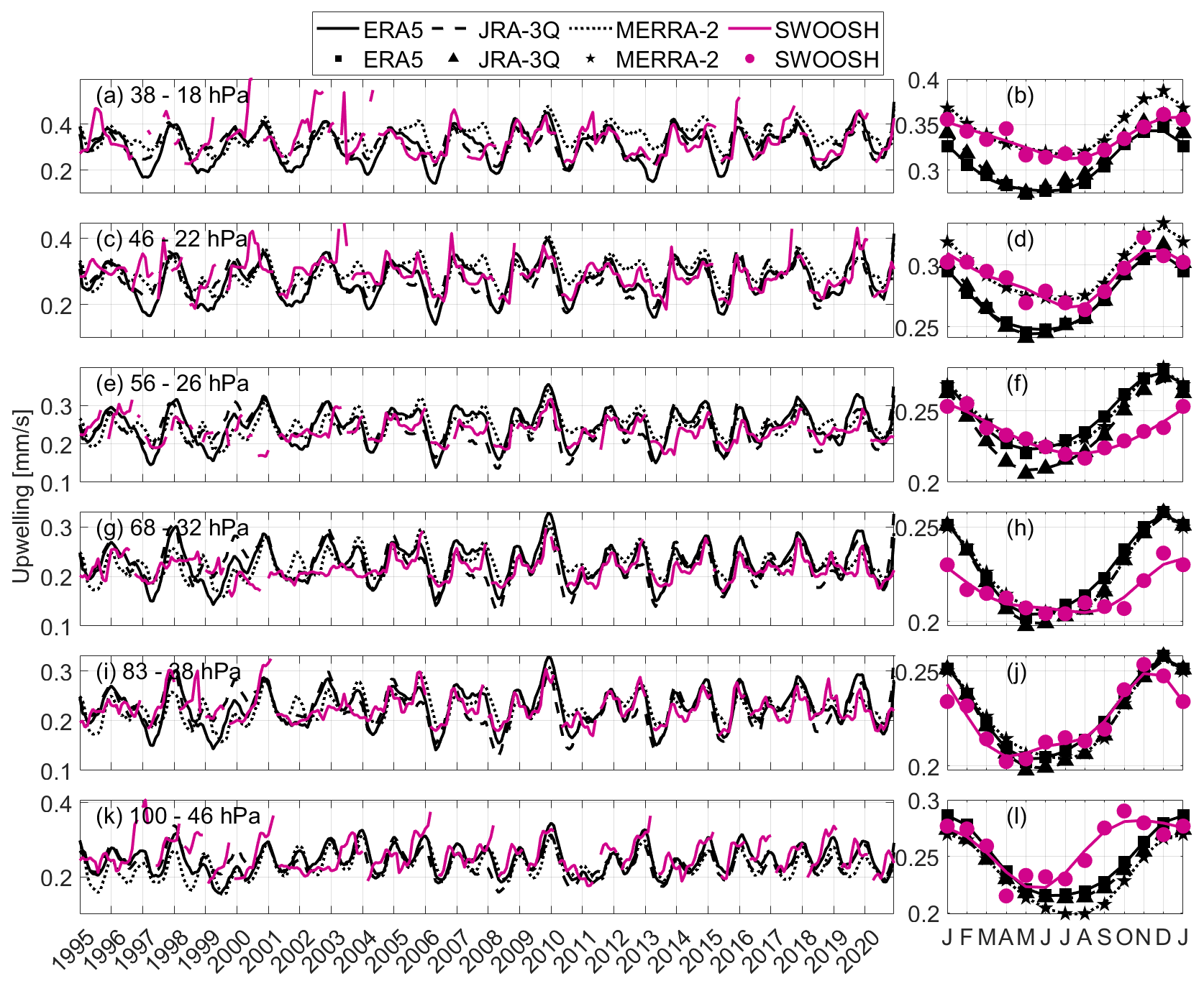
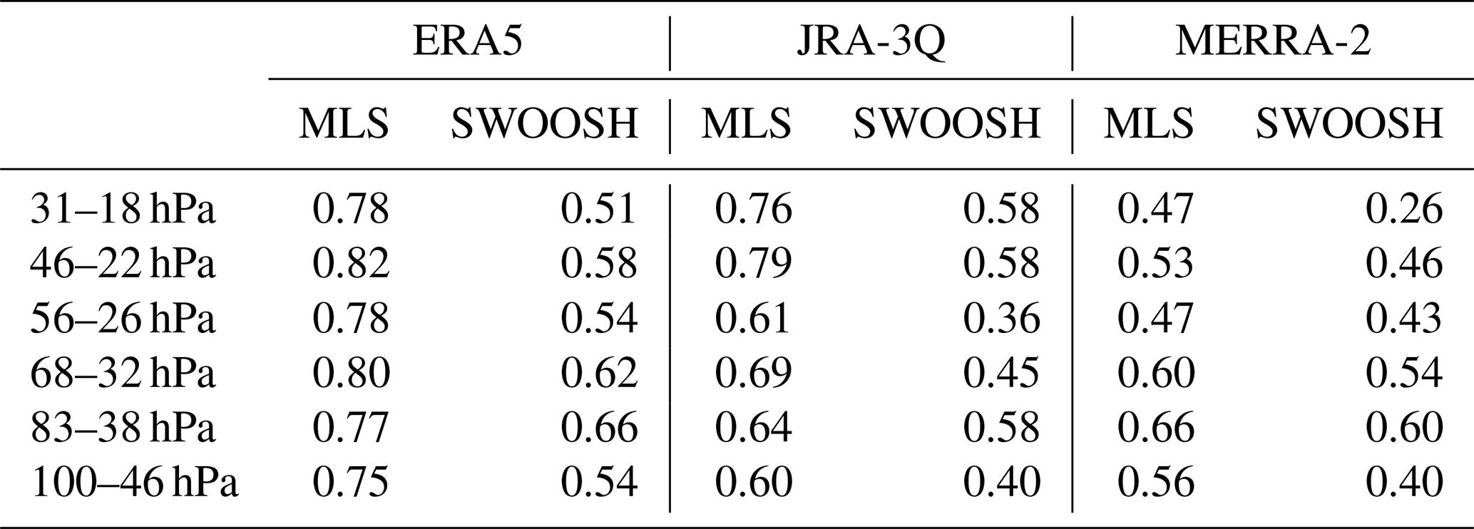
As explained in Sect. 2.3, applying the time-lagged correlation method for 6 month long sections of the time series allows for the seasonal cycle of upwelling to be obtained. This analysis was performed for the MLS and SWOOSH water vapour, and the resulting time series and corresponding seasonal cycles are shown in Figs. 8 and 9, respectively. For comparison, the vertical component of the residual circulation calculated from ERA5, JRA-3Q, and MERRA-2 were smoothed with a 7 month running average to match the temporal resolution of the time-lagged correlation method and were plotted with the upwelling. Thus, the seasonal cycles are derived from these smoothed time series, rather than the original monthly resolution time series. The reanalysis is given as a mean over 10° S–10° N and 18° S–18° N for comparison with MLS and SWOOSH, respectively. The correlation coefficients describing the similarity between the MLS and SWOOSH time series with each of the reanalysis are shown in Table 1. For MLS, there is good agreement in the range of 0.75 to 0.82 with ERA5, 0.60 to 0.79 with JRA-3Q, and weaker agreement in the range of 0.47 to 0.66 with MERRA-2. The agreement with each of the reanalysis for SWOOSH ranges from 0.51 to 0.66 for ERA5, 0.36 to 0.58 for JRA-3Q, and 0.26 to 0.60 for MERRA-2. In general, the upwelling estimate calculated from MLS correlates better with the reanalysis than that from SWOOSH. If this comparison is performed by taking SWOOSH data for the MLS period only (not shown), the correlation coefficients are found to be comparable to those from the MLS data, further demonstrating the higher uncertainty for the period before 2005.

Table 1 Correlation coefficient (R) for upwelling calculated from MLS and SWOOSH water vapour using the 6 month lagged correlation method with the vertical component of the residual circulation from ERA5, JRA-3Q, and MERRA-2 reanalysis smoothed over 7 months.

In addition to finding good agreement in terms of interannual variability between the lag-correlation calculated upwelling and reanalysis residual circulation, there is also reasonable agreement in the timing of the seasonal cycles. Both our estimates and the reanalysis find a seasonal cycle which maximizes in boreal winter and minimizes in boreal summer, as is expected for the vertical residual mean meridional circulation in the tropical stratosphere (e.g. Rosenlof, 1995). With a few exceptions, in general our estimated upwelling is stronger in the seasonal mean than the reanalyses, and the overall cycle is flatter with less distinction between the seasonal maximum and minimum. These are features that would be expected to appear as a result of the inclusion of mixing in our transport estimate. Mixing acts to blur together the water vapour signal at consecutive levels, giving a decreased lag in the tape recorder signal, and a faster estimate of upwelling (Mote et al., 1998). Therefore, our estimate is found in general to be stronger than the reanalyses, and the enhanced influence of mixing in the NH summer season reduces the extent to which we see a decrease in summertime upwelling in our estimate.

As is evident in Figs. 8 and 9 and in the correlation coefficients between the individual reanalyses and the MLS and SWOOSH upwelling estimates, MERRA-2 stands out as having poorer agreement when compared with ERA5 and JRA-3Q, especially when compared with MLS and at the higher levels. This is seen in the variability of the time series, where MERRA-2 appears to be shifted in time relative to the other upwelling estimates for certain portions of the time series, in the seasonal cycle, where MERRA-2 is significantly weaker for the lowest layers and the minimum is shifted slightly forward in time for the lowest layer, and for the profile, where MERRA-2 stands farther apart from the other estimates above about 41 hPa. The differences between the individual reanalyses can be ascribed to the differences in the reanalysis schemes which impact how atmospheric structures important for the calculation of the residual circulation are resolved (SPARC, 2022; Fujiwara et al., 2024).

3.4 Upwelling and ANCISTRUS vertical transport

ANCISTRUS provides another estimate of upwelling in the stratosphere. The ANCISTRUS vertical velocities are similar to our lag-correlation calculated vertical velocities in that satellite observations are used to infer transport in the stratosphere, and the resulting transport speeds are an effective estimate which include the impact of both advection and mixing. However, unlike our lag-correlation method the ANCISTRUS scheme uses measurements of a number of long-lived tracers (H₂O in addition to SF₆, CFC-11, CFC-12, HCFC-22, CCl₄, N₂O, CH₄, and CO) from the Michelson Interferometer for Passive Atmospheric Sounding (MIPAS) satellite instrument, and infers the meridional circulation of the stratosphere and mesosphere through the inversion of the 2-D continuity equation for tracer mixing ratio and air density (von Clarmann et al., 2021). The vertical velocities produced by ANCISTRUS represent effective velocities that include effects both from advection and mixing, similar to the effective velocities derived from the lag-correlation method, however through the use of different tracers and with a different method. Because of the differences between the lag-correlation method and ANCISTRUS, the implicit inclusion of mixing in the circulation calculation impacts the resulting velocities differently. Whereas for the water vapour lag-correlation calculation the assumption is that the influence of mixing is to in general overestimate the vertical velocity, the same cannot be assumed for the ANCISTRUS velocities. Instead, for ANCISTRUS the impact of mixing could be to produce either an over- or underestimation of the true vertical velocity.

Based on the results of Mote et al. (1998), we expect the impact of mixing on our lag-correlation calculated estimates to be negligible in the region below 25 km but become more significant at higher altitudes. The ANCISTRUS vertical velocities are shown in a profile along with the upwelling estimates from the 12 month lag-correlation method using MLS data in Fig. 10. Here the ANCISTRUS data is taken in a tropical mean over 12° S to 12° N. We note that in the altitude range shown in Fig. 10, the 3 km ANCISTRUS grid contains only two vertical levels (21 and 24 km). As a result, the retrieved vertical structure is necessarily smooth and limited by the rather coarse discretization in this application. We find good agreement between the two estimates between about 20 and 24 km altitude. Below and above this region, the profiles diverge with the ANCISTRUS profile taking on smaller values than our MLS estimate. The dissimilarity in the profiles above 24 km could be a result of an increased influence of mixing, appearing as opposite tendencies in the calculations from the two methods. Below 20 km the observed difference could again be a reflection of the influence of mixing but could also be impacted by a rather strong vertical regularization used in the current ANCISTRUS version. This regularization could be strongly tying the velocities in the lower troposphere to zero, resulting in the decrease in the profile visible in Fig. 10.

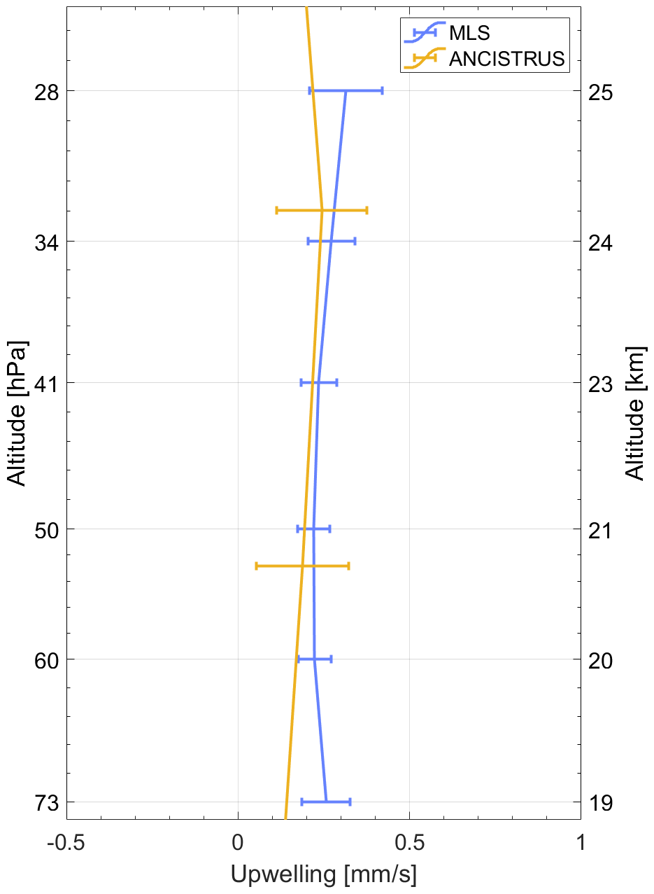
Figure 10 Profile of upwelling for ANCISTRUS and the MLS method. Horizontal bars give the uncertainty range derived as the 2σ standard deviation of the monthly time series.

To further assess our estimate against the ANCISTRUS velocities, we compare the temporal variability from both the 6 and 12 month correlation methods. Figure 11 shows time series of our MLS vertical velocities along with ANCISTRUS correspondingly smoothed over 7 and 13 months to match with the temporal resolution of the MLS estimates. The velocities output from the ANCISTRUS model are gridded in latitude and height. For comparison of the time series, the ANCISTRUS data were chosen such that the altitude best matches the midpoint of the layers used in the MLS calculation. The temporal smoothing of ANCISTRUS was necessary to match the resolution of the MLS calculated upwelling and suppresses much of the sub-seasonal variation. The muted seasonality in ANCISTRUS therefore reflects the temporal averaging rather than a limitation of the method.

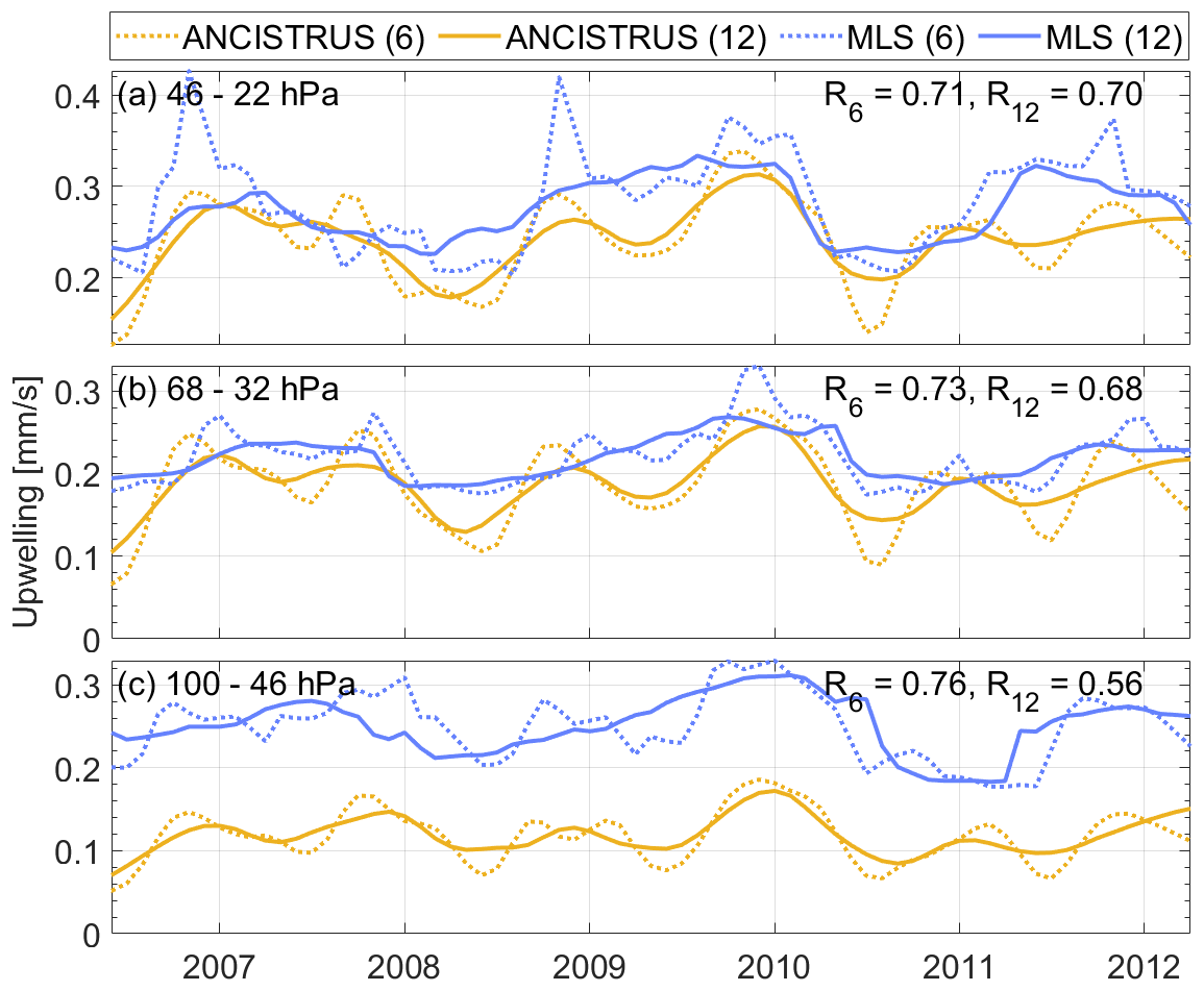
Figure 11 Time series of upwelling from ANCISTRUS and the MLS method for (a) ANCISTRUS at 24 km and MLS over 46–22 hPa (midpoint of about 24 km), (b) ANCISTRUS at 21 km and MLS over 68–32 hPa (midpoint of about 21 km), and (c) ANCISTRUS at 18 km and MLS over 100–46 hPa (midpoint of about 19 km). Uncertainty shading is omitted here to simplify the figure. The labels (6) and (12) in the legend denote the 6 month and 12 month methods for the MLS data, and corresponding smoothing in the ANCISTRUS data. The values shown for R₆ and R₁₂ are the correlation coefficients between MLS and ANCISTRUS for the 6 month and 12 month methods and corresponding smoothing.

We find good agreement in terms of variability for the time series compared in Fig. 11, the correlations for the 12 month smoothing are found to be 0.71, 0.73, and 0.76 for Fig. 11a–c respectively, and similarly for the 6 month smoothing these values are found to be 0.70, 0.68, and 0.56. As is found in the comparison of the profile, the ANCISTRUS velocities are lower than MLS, strongly at 18 km, and less so at 21 and 24 km. The good agreement found here further demonstrates the robustness of these methods for estimating tropical upwelling in the region between 20 and 24 km altitude, albeit with some differences in strength as a result of differences in the methods. The good agreement does not exclude the possibility that both methods are impacted by the effects of mixing.

4 Conclusions

We have generated a time series of the effective vertical transport velocity in the tropical lower and middle stratosphere based on 16 years of MLS and 27 years of SWOOSH water vapour data. This method uses the time lag of the tape recorder signal between subsequent levels to calculate the effective vertical velocity, which approximates the residual vertical velocity if mixing has a negligible influence on the signal. Previous studies such as Mote et al. (1998) have shown that the latter has only a small influence on the derived effective velocity in the region considered here.

We find good agreement between our estimates from the daily MLS data and 5 d resolution SWOOSH data for the period over which they overlap in both the climatological mean and interannual variability. This demonstrates the ability of the lag-correlation method to obtain reasonable upwelling estimates from the data with more coarse temporal gridding. Due to noise and sparsity of observations in the SWOOSH record prior to Aura MLS, the calculations from SWOOSH water vapour in the period between 1995 and 2005 have a larger uncertainty.

Identifying the mechanisms forcing variability in upwelling provides an important contribution to our understanding of past and future circulation changes. A regression analysis was performed to assess the strength of the QBO, ENSO, volcanic forcing, and solar cycle signals in the variability of the calculated upwelling. From this analysis, we found that a large amount of variability is captured by the regression model, with $R_{\text{adj}}^{\mathrm{2}}$ throughout the lower and middle stratosphere for MLS in the range of 0.59 and 0.72, and for SWOOSH between 0.41 and 0.57. The largest signal is coming from the QBO term, which dominates the explained variability of tropical upwelling. ENSO is found to have a significant contribution to the explained variability only below 41 hPa, with the QBO and ENSO being equally important in the lowermost stratosphere. The signal from volcanic forcing was found to be not significant for both data sets and time periods, which could be a result of the lack of significant eruptions in the time period considered here. The signal from the solar cycle is only significant for SWOOSH, likely owing to the significantly longer data record, and could be related to a multi-decadal signal in upwelling.

Our analysis reveals a peak of strongly enhanced upwelling in the lower stratosphere in late 2000/early 2001 that cannot be explained by QBO or ENSO variability. This enhanced tropical upwelling coincides with the onset of a drop in water vapour and cold point temperatures at the same time (Randel et al., 2006) suggesting that these were at least partially driven by lower stratospheric upwelling changes. Similarly, there is a strong decrease in upwelling from mid-2010 to mid-2011, which can be only partially explained by the QBO and ENSO driven regression terms. This decrease in upwelling is consistent with an increase in stratospheric water vapour in 2011.

We use independent observational data to show that tropical upwelling is anticorrelated with long-lived stratospheric tracers such as ozone. A comparison of our calculated upwelling with ozone from OSIRIS produces the expected strong anti-correlations with coefficients ranging between −0.63 and −0.84 for the levels considered here. Features of reduced variability present in the upwelling, ozone, and upwelling regression fit post 2015 are consistent with similar features in the QBO temperature signal and are shown to be likely an outcome of the QBO disruptions in 2015/16 and 2019/20. Similar results are found when comparing the MLS upwelling with ozone measured by the MLS instrument, and from comparisons of the SWOOSH upwelling with both MLS and OSIRIS ozone.

Given uncertainties in modelled upwelling as a result of a lack of observations, we compared our estimates to the calculated residual meridional circulation from reanalysis to test for consistencies in the interannual variability, seasonal cycle, and climatological mean. The vertical component of the residual meridional circulation calculated from ERA5, JRA-3Q, and MERRA-2 is found to agree well with our estimates in the climatological mean, interannual variability, and in the seasonal cycle. Differences are largest for MERRA-2, indicating that the upwelling time series for the regions considered here deviates slightly from that in ERA5, JRA-3Q, and our estimates. These results reaffirm confidence in the reanalysis upwelling estimates, with the caveat that methodological uncertainties exist in our estimated upwelling as discussed in Sects. 2.3 and 3.3 potentially hindering an accurate direct quantitative comparison as exemplified by the differences in upwelling strength shown in the seasonal cycles of Figs. 8 and 9.

The ANCISTRUS calculation scheme provides another independent estimate of tropical upwelling. We compared the vertical component of the meridional circulation from ANCISTRUS with our upwelling estimates calculated from MLS in both the profile and time series. We found good agreement in the shape of the profile between 20 and 24 km altitude, and good agreement of interannual variability at all levels. The disagreement in the profile above and below the 20 to 24 km region can be attributed to the impact of mixing, which affects each calculation differently, and the regularization scheme applied in ANCISTRUS.

The degradation of the MLS water vapour measurement frequency to about six measurements per month in 2024 in an attempt to prolong the lifetime of the instrument marks the beginning of a dearth of high-resolution satellite observations of water vapour. While SAGE III/ISS provides water vapour profiles that extend through the stratosphere in addition to MLS, the future extension of this mission remains uncertain at this time. This gap in high-resolution measurements in the water vapour record has no prospect of ending until the planned launch of the High-altitude Aerosols, Water Vapour and Clouds (HAWC) mission Spatial Heterodyne Observations of Water (SHOW) instrument around 2031 (Langille et al., 2025). The absence of dense measurements limits the study of the BDC through analysis as presented here, reducing the number of methods through which the variability of tropical upwelling can be observed and understood for the period of the data gap.

Appendix A

In Sect. 3.1, two examples were looked at when discussing the regression fits and residuals for the regression of the upwelling calculated from MLS and SWOOSH water vapour. For the interest of the reader, we include these plots for both instruments at all six levels in Fig. A1 here.

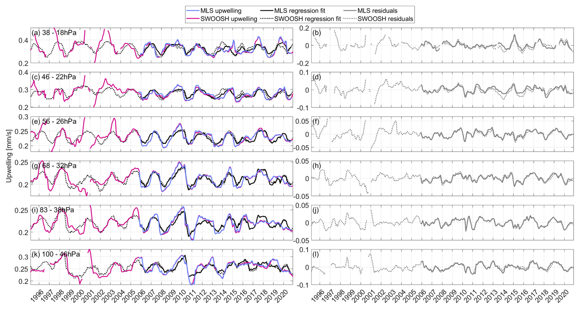
Figure A1 Time series of regression fits and residuals for MLS and SWOOSH at (a, b) 38–18 hPa, (c, d) 46–22 hPa, (e, f) 56–26 hPa, (g, h) 68–32 hPa, (i, j) 83–38 hPa, and (k, l) 100–46 hPa.

Appendix B

As described in Sect. 3.2, we chose to correlate the upwelling and ozone taking ozone at the top level of the upwelling layer. Figure B1 demonstrates the results if instead ozone is taken in a mean over the upwelling layer. We still find reasonably strong correlations in the upper levels, but these correlations become weaker below the 56–22 hPa layer and are very weak for 83–38 hPa.

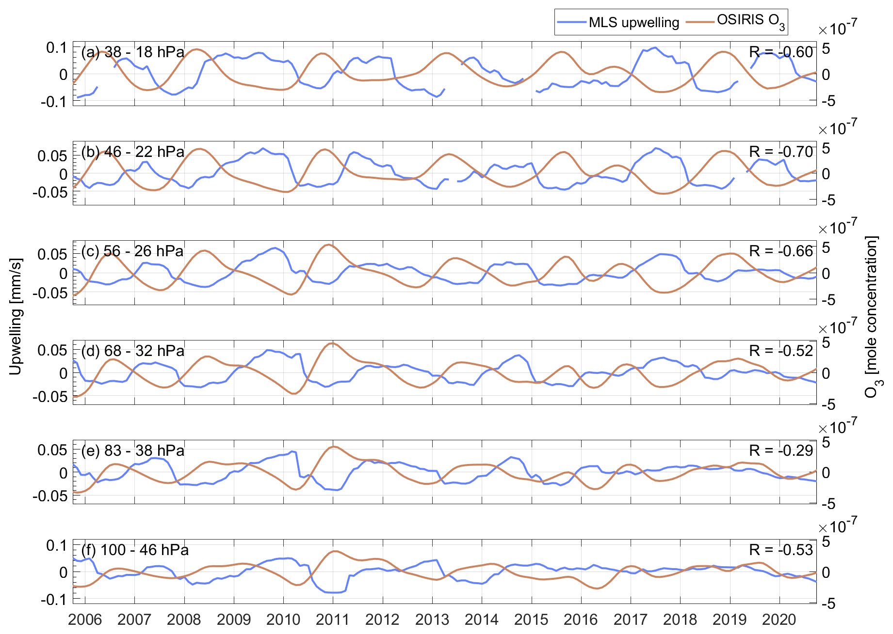
Figure B1 Time series of upwelling anomalies from MLS plotted along with O₃ anomalies from OSIRIS for (a) MLS between 38–18 hPa and OSIRIS O₃ between 22.5–27.5 km (about 38–18 hPa); (b) MLS between 46–22 hPa and OSIRIS O₃ between 21.5–26.5 km (about 44–20 hPa); (c) MLS between 56–26 hPa and OSIRIS O₃ between 20.5–24.5 km (about 52–27 hPa); (d) MLS between 68–32 hPa and OSIRIS O₃ between 18.5–23.5 km (about 73–33 hPa); (e) MLS between 83–38 hPa and OSIRIS O₃ between 17.5–22.5 km (about 87–37 hPa); and (f) MLS between 100–46 hPa and OSIRIS O₃ between 16.5–21.5 km (about 103–45 hPa).

Similar to ozone, higher tropospheric values of hydrogen chloride (HCl) produce an inverse relationship with upwelling (e.g. Mahieu et al., 2014). Anomalies of tropical upwelling calculated from MLS using the 12 month lag-correlation method are plotted with tropical mean (10° S to 10° N) HCl measured by MLS in Fig. B2. The HCl time series is smoothed with a 13 month moving mean to match the temporal resolution of upwelling. The correlation coefficients between the upwelling and HCl are found to be −0.59, −0.57, and −0.37 for the 46–22 hPa, 68–32 hPa, and 100–46 hPa levels, respectively.

Figure B2 Time series of upwelling anomalies from MLS plotted along with HCl anomalies from MLS for (a) upwelling between 46–22 hPa and HCl at 22 hPa; (b) upwelling between 68–32 hPa and HCl at 32 hPa; and (c) upwelling between 100–46 hPa and HCl at 46 hPa.