Quantifying and addressing the uncertainties in tropospheric ozone and OH in a global chemistry transport model

The major physical and chemical processes governing the abundance of atmospheric oxidants such as ozone and hydroxyl radicals (OH) are largely understood, but quantitative assessment of their importance in different environments remains challenging. Atmospheric chemistry transport models allow exploration of these processes on a global scale, but weaknesses in process representation in these models introduces uncertainty, and model intercomparisons show considerable diversity even in representing current atmospheric composition. Formal constraint of models with atmospheric observations is needed to provide more critical insight into the causes of model weaknesses. In this study we perform a global sensitivity analysis on a chemistry transport model using Gaussian process emulation and identify the processes contributing most to uncertainty in tropospheric ozone and OH. We then explore the use of atmospheric measurements to calibrate the model and identify weaknesses in process representation and understanding. We find that the largest uncertainties are associated with photochemical kinetic data and with factors governing photolysis rates and surface deposition. Calibration constrains the uncertainty in key processes, improving comparisons with observations and informing model development, but we show that it is also valuable in identifying structural errors in models. We show that surface ozone measurements alone provide insufficient constraint, and we highlight the importance of applying a broad range of different observational metrics. While this study is exploratory in nature, focussing on a limited number of constraints, we clearly demonstrate the value of rigorous calibration for providing important new insight into key processes and their representation in atmospheric models.

1 Introduction

Tropospheric ozone is an important pollutant of major policy concern due to both its impacts on human health and vegetation at the Earth's surface and to its role as a greenhouse gas contributing to climate change (Monks et al., 2015). The main physical and chemical processes controlling its formation, transport and fate are largely understood, and these are represented in the global and regional atmospheric, climate and earth system models that are used to investigate its distribution, trends and broader environmental impacts (Young et al., 2018). However, there are still substantial differences between models in their assessment of the tropospheric ozone burden and in estimates of the tropospheric chemical lifetime of methane, which provides an integrative measure of the hydroxyl radical (OH) that governs most tropospheric oxidation processes (Wild, 2007; Voulgarakis et al., 2013; Young et al., 2018). These global metrics are vital in understanding the long-term evolution of tropospheric composition driven by pollutant emissions and climate change, and the diversity in model results undermines confidence in our assessment of these changes. In addition, global and regional models often show substantial biases in representing ozone concentrations at the surface of the Earth, and this reduces their value in assessing damage to natural vegetation, crop production and human health (Young et al., 2018; Gaudel et al., 2018). A better understanding of the sources of model diversity is needed, both to identify weaknesses in current understanding of key processes and their representation in models, and to provide improved quantification of the uncertainty in simulated impacts on the environment.

The importance of different physical and chemical processes in governing atmospheric composition can be explored with simple model sensitivity studies investigating one process at a time (e.g. Wild, 2007). However, more rigorous global sensitivity analysis across multiple variables is now becoming computationally feasible, and has been used to explore atmospheric aerosol processes (Lee et al., 2011, 2013), tropospheric composition (Ryan et al., 2018; Derwent et al., 2018), the atmospheric methane budget (Stell et al., 2021) and the effect of emissions and chemical processes on surface air quality (Beddows et al., 2017; Aleksankina et al., 2019) and on aircraft measurements (Christian et al., 2018). These approaches can be extended to a more formal assessment of model uncertainty, and studies have explored the effects of uncertainty in aerosol processes on radiative forcing (Johnson et al., 2020), in chemical reaction rates on tropospheric oxidant concentrations (Newsome and Evans, 2017; Ridley et al., 2017) and in physical and chemical processes on regional surface ozone (Dunker et al., 2020). While quantification of uncertainty is valuable in assessing confidence in model simulations, it also provides an opportunity to calibrate models against atmospheric observations, to constrain process uncertainty and to identify weaknesses in process representation or in current process understanding. Formal statistical constraints have been used to improve understanding of the role of aerosol processes in radiative forcing (Regayre et al., 2020; Johnson et al., 2020) and to identify structural inconsistencies in climate models (Regayre et al., 2023), but have not previously been used to investigate tropospheric oxidation processes.

This study provides the first thorough assessment of the major sources of uncertainty in representing tropospheric ozone and OH across a wide range of physical and chemical processes. In an exploratory study focussing on a few selected processes we demonstrated the value of Gaussian process emulation for performing global sensitivity analysis of atmospheric models and for diagnosing the cause of differing model responses (Wild et al., 2020). Here we consider a much broader set of processes and quantify process uncertainty across them in a more self-consistent manner, identifying the processes making the largest contribution to uncertainty in modelled ozone and OH. We then explore how atmospheric measurements may be used to constrain process uncertainty in models, identifying both model weaknesses and refinements needed to provide more robust constraints.

2 Model and Approach

For this study we use the Frontier Research System for Global Change version of the University of California Irvine Chemical Transport Model (FRSGC/UCI CTM) as described in Wild (2007). The model was developed to represent tropospheric gas-phase processes and is run at T42 (2.8° × 2.8°) resolution with 37 vertical levels between the surface and 64 km driven by meteorological fields from the European Centre for Medium-Range Weather Forecasts (ECMWF) Integrated Forecasting System (IFS). Meteorological fields for 2001 were used for this study, with anthropogenic emissions for 2000 taken from EDGAR v3.2 as described in Stevenson et al. (2006). This configuration of the model is the same as that applied in the Hemispheric Transport of Air Pollution (HTAP) model intercomparison (Fiore et al., 2009; Wild et al., 2012) and has been used in previous studies investigating the sources of uncertainty in tropospheric chemistry and composition (Wild et al., 2020; Ryan and Wild, 2021). The model includes explicit treatment of HO_x/O_x/NO_x chemistry and CH₄ oxidation and has a lumped chemistry for representative alkane, alkene and aromatic species and isoprene. The only changes for this study are inclusion of the reaction of hydrogen with hydroxyl radicals, a substantial sink of OH that was omitted in earlier studies, and incorporation of a monthly-mean aerosol climatology to provide temporally and spatially-varying aerosol optical depth profiles for photolysis rate calculations. The combined effect of these changes is an increase in the chemical lifetime of methane by 0.6 years, from 8.7 to 9.3 years, driven mostly by the inclusion of hydrogen, and a small increase in tropospheric ozone burden from 316 to 318 Tg. Both of these changes bring the model into closer agreement with observations. The model does not have an interactive treatment of aerosol processes, and therefore we only consider the impacts of aerosol through their influence on photolysis rates and heterogeneous chemistry. The model is run in offline mode driven by meteorological reanalyses, so changes in atmospheric composition do not influence meteorological processes. The interaction of atmospheric composition with meteorological and transport processes provides additional sources of uncertainty that are not explored here.

We first explore the importance of different processes using a simple one-at-a-time sensitivity analysis. This allows identification of the key processes to consider and provides an estimate of their impacts relative to the standard model control run. However, global sensitivity analysis requires a more thorough assessment that accounts for the interactions between processes and for non-linearity in model responses, and any subsequent model calibration requires detailed exploration of the resulting parameter space. These approaches typically require many thousands of model runs to cover the parameter space, and are too computationally demanding to perform with a global CTM. We therefore apply a surrogate model, a statistical model that maps the input-output relationships of the computationally expensive CTM. We use a Gaussian process (GP) emulator as the surrogate model in these studies as this has attractive statistical properties (e.g., allowing direct assessment of the uncertainty in the emulated output) and has been shown to successfully mimic the input-output behaviour of complex models such as CTMs to a high degree of accuracy (Lee et al., 2011; Ryan et al., 2018).

For evaluation and constraint of the model, we use measurements of ozone from surface locations and the mid-troposphere. We use surface measurements contributed to the Tropospheric Ozone Assessment Report (TOAR) database, which provides a quality-controlled and globally consistent dataset of long-term surface ozone observations (Schultz et al., 2017a). We use the monthly-mean gridded observational product at 64 locations across the globe with sufficient data for 2001. The TOAR database provides statistics for rural and urban measurement sites, and we use observations from rural sites where available, as these better reflect the regional characteristics of ozone that we are able to represent with the CTM. We select the coarse 10° × 10° gridded product to reduce dependence on individual measurement sites and to capture the large-scale spatial variability of ozone while keeping the number of data points to a minimum, although we note that there is some associated loss of spatial information. For the troposphere, we use the Trajectory-mapped Ozonesonde dataset for the Stratosphere and Troposphere (TOST) ozone climatology (Liu et al., 2013). We use monthly-mean gridded ozone mixing ratios at 10° × 10° resolution at 5.5 km altitude (roughly 500 hPa) to represent the mid-troposphere. As observations for 2001 are relatively sparse at many locations, we take a 5-year average over the 1999–2003 period, and use the smoothed ozone product to reduce sampling noise. We select locations at or close to ozonesonde launch sites where data coverage is good, and choose a total of 64 locations to match the number of surface observation sites available from TOAR.

To provide additional constraints on the model simulations we apply observation-based estimates of the global tropospheric ozone burden and the tropospheric chemical lifetime of methane. The global tropospheric ozone burden is the annual mean mass of ozone below the tropopause, defined here as the 150 ppb isosurface of ozone, and this has been estimated from ozonesonde climatologies at 335±10 Tg (Wild, 2007) and 338±8 Tg (Gaudel et al., 2018). Recent multiple model ensemble studies find a burden of 340±34 Tg, suggesting that it is represented relatively well in current models (Young et al., 2018). The tropospheric chemical lifetime of methane is defined as the global mean atmospheric burden of methane divided by the total annual loss to chemical removal by reaction with OH in the troposphere. This has been derived from a thorough observation-based sensitivity analysis as 11.2±1.3 years (Prather et al., 2012), and is typically underestimated in models by about 15 %, e.g., 9.8±1.6 years in the ACCMIP model intercomparison (Voulgarakis et al., 2013). For these global metrics, the tropospheric ozone burden from the standard control run of the FRSGC/UCI CTM lies somewhat below the observation-based value, at 318 Tg, and the methane chemical lifetime is also low, at 9.3 years, but both metrics lie well within the range seen in recent model studies.

Table 1 Model parameters investigated in the study. Multiplicative factors are applied as linear scalings (full range: ± x %) or as logarithmic scaling factors (full range: $\mathrm{1}/y$ to y). The 36 most important parameters (starred) are selected for further analysis.

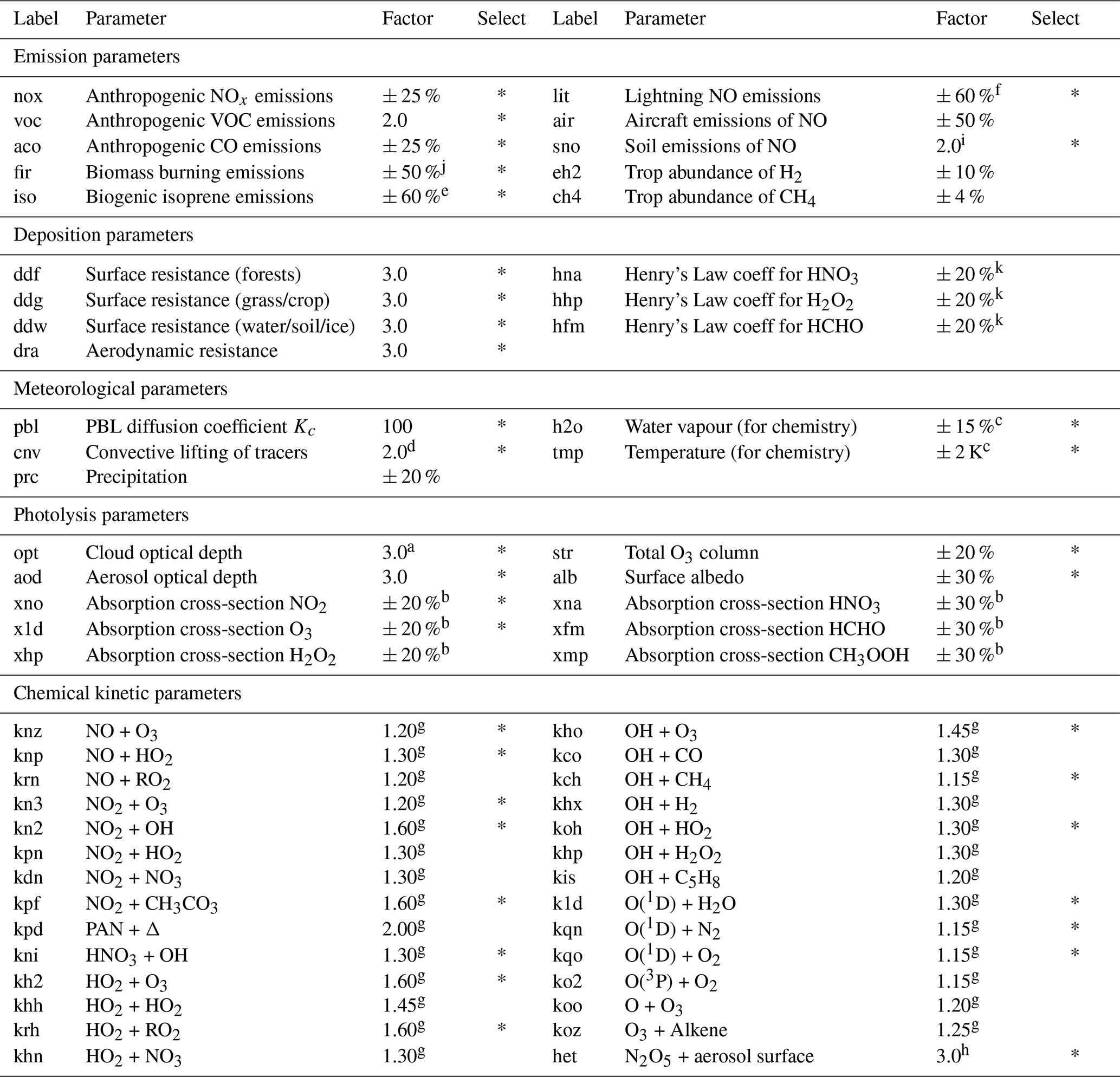
References: ^a Klein et al. (2013). ^b Burkholder et al. (2015). ^c Hearty et al. (2014). ^d Hoyle et al. (2011). ^e Ashworth et al. (2010). ^f Schumann and Huntrieser (2007). ^g Atkinson et al. (2004). ^h Macintyre et al. (2010). ⁱ Weng et al. (2020). ^j Wiedinmyer et al. (2023). ^k Sander (2023).

3 Sources of model uncertainty

Uncertainty in model simulations arises from model inputs, such as emissions data, from model parameterizations associated with the representation of specific processes, and from structural issues associated with numerical algorithms, discretization and spatial and temporal resolution. We focus here on model inputs and parameters, noting that exploration of structural uncertainties would be valuable for a comprehensive analysis. Given the large number of independent parameters included in chemistry-transport models, we adopt a pragmatic approach that addresses the largest sources of uncertainty in key processes but avoids low-level, parameterization-specific uncertainties that would make it very difficult to reproduce the results with other models. We focus here on emissions, deposition, meteorology and photochemical processes that are important for tropospheric oxidant budgets, and aim for a consistent quantitative definition of uncertainty that is broadly representative of a ±2σ variation. We take estimates of uncertainty from the literature wherever possible, but supplement this with expert elicitation for processes or parameters for which uncertainty is less well characterised. The 60 parameters considered here are listed in Table 1.

3.1 Processes and parameters investigated

Uncertainty in the emissions of ozone precursors is often the first subject of attention when model simulations do not match observations. Key trace gases such as NO_x, CO, VOC and CH₄ have both anthropogenic and natural sources, many of which vary strongly in space and time, influencing local and regional ozone production. To reduce complexity, we consider uncertainty in the total magnitude of global emissions, but neglect uncertainty in their temporal and spatial distribution. We consider anthropogenic surface sources of NO_x, VOC and CO, lightning, soil and aircraft sources of NO, biogenic emissions of VOC (represented here by isoprene), and biomass burning emissions. Few inventories come with rigorous estimates of uncertainty, so we base our assessments on expert judgement and on differences between existing inventories as assessed in previous studies (e.g. Hoesly et al., 2018; Wiedinmyer et al., 2023). We assume an uncertainty of  ± 25 % for global anthropogenic surface NO_x and CO emissions,  ± 50 % for biomass burning and aircraft emissions,  ± 60 % for biogenic and lightning emissions, and a factor of two for soil NO and surface VOC emissions, see Table 1. To aid reproducibility with other models we have use standardised base emissions of 30 TgN yr⁻¹ for surface anthropogenic NO_x emissions, 600 Tg yr⁻¹ for surface anthropogenic CO emissions, 500 TgC yr⁻¹ for biogenic isoprene emissions and 5 TgN yr⁻¹ each for lightning and soil NO_x emissions. Longer-lived precursors such as H₂ and CH₄ are given fixed tropospheric abundances in the model (500 ppb for H₂ and 1760 ppb for CH₄ in this study, corresponding to year 2000 conditions), and uncertainties in these abundances are considered here in place of emissions uncertainty.

Deposition processes remain highly uncertain, and have been shown to make a major contribution to differences in global model simulations of oxidants (Hardacre et al., 2015). Following the resistances approach described by Wesely (1989), from which most model dry deposition schemes are derived, we focus on the aerodynamic resistance, representing the transport of trace gases to the surface, and the surface resistance, representing removal of gases on surfaces through physical, chemical or biological processes. We lump surface land cover class by vegetation type, distinguishing heavily vegetated surfaces (e.g., forests) from those with moderate vegetation (grassland and crops) and little or no vegetation (water, desert, ice or snow). We consider uncertainty in the surface resistances over these three land cover classes separately, assuming a range of a factor of three, and apply these to all species undergoing dry deposition. The broad range used here is intended to accommodate the diversity of approaches adopted for surface uptake, which differ greatly in complexity across models (Clifton et al., 2020). For wet deposition, we consider uncertainty in the solubility of the key oxidants HNO₃, H₂O₂ and HCHO through their Henry's Law coefficients which are known to about  ± 20 % (Sander, 2023), and we consider uncertainty in total annual precipitation as a meteorological variable.

Uncertainty in meteorological and dynamical processes is difficult to assess here as we use an offline model driven by pre-calculated meteorological fields and are therefore not able to perturb parameters in a physically self-consistent way. However, the maximum uncertainty in the representation of temperature in climate models is about 2 K (Hearty et al., 2014), and the corresponding uncertainty in water vapour is about  ± 15 %, and we apply these to the chemical processes represented in the model. We also investigate uncertainty in model precipitation, which influences the wet scavenging of soluble species. Quantifying uncertainty due to dynamical processes is challenging in an offline model, but we consider the convective lifting of trace species, which plays a key role in controlling the lifetime and distribution of oxidants, and which has an uncertainty of about a factor of two (Hoyle et al., 2011). We note that we are not able to explore uncertainties in the strength and depth of convection, which may also be of interest. Turbulence in the atmospheric boundary layer is important in governing oxidant concentrations at the Earth's surface. Previous model studies have taken a range of approaches from assuming immediate vertical mixing through the depth of the boundary layer to neglecting it completely, relying on numerical mixing to serve as a proxy. Here we calculate an effective vertical diffusion coefficient for mixing through the depth of the boundary layer, and assume a large uncertainty so that turbulent mixing between model layers varies from negligible to almost complete at each time step.

Photolysis is important for initiating atmospheric photochemistry, and solar radiation reaching the troposphere is dependent on the stratospheric ozone column and the optical depth associated with clouds and aerosol. While the global average total ozone column is reasonably well constrained, there are large latitudinal and seasonal variations, and model-derived columns diverge from standard climatologies, so we adopt a maximum uncertainty of  ± 20 %. We apply a factor of three uncertainty in cloud optical depth, following Klein et al. (2013), and adopt the same uncertainty for aerosol optical depth. Experimentally-determined absorption cross-sections for key oxidants have uncertainties in the range  ± 20 %–30 % (Burkholder et al., 2015) and we consider these for NO₂, O₃, and other key species including H₂O₂, HNO₃, HCHO and CH₃COOH.

Uncertainty in photochemical reaction parameters is relatively well characterised in existing kinetic data evaluations (Atkinson et al., 2004; Burkholder et al., 2015), and we adopt an uncertainty range of ±2σ for consistency with the physical parameters considered here. We apply these independently to all reactions in the model chemistry scheme that have a substantial impact on ozone or OH. Uncertainty is characterised by a γ term in Atkinson et al. (2004) (where 2σ=10^γ) and by a f term in Burkholder et al. (2015) (where 2σ=f²), and in the rare cases where these differ substantially we have favoured the recommendation of Atkinson et al. (2004) to maintain consistency with the standard kinetic data used in the model chemistry scheme. We neglect the additional effects of uncertainty associated with the temperature dependence of the rate constants, which was included in the study of Newsome and Evans (2017), to keep the number of parameters manageable.

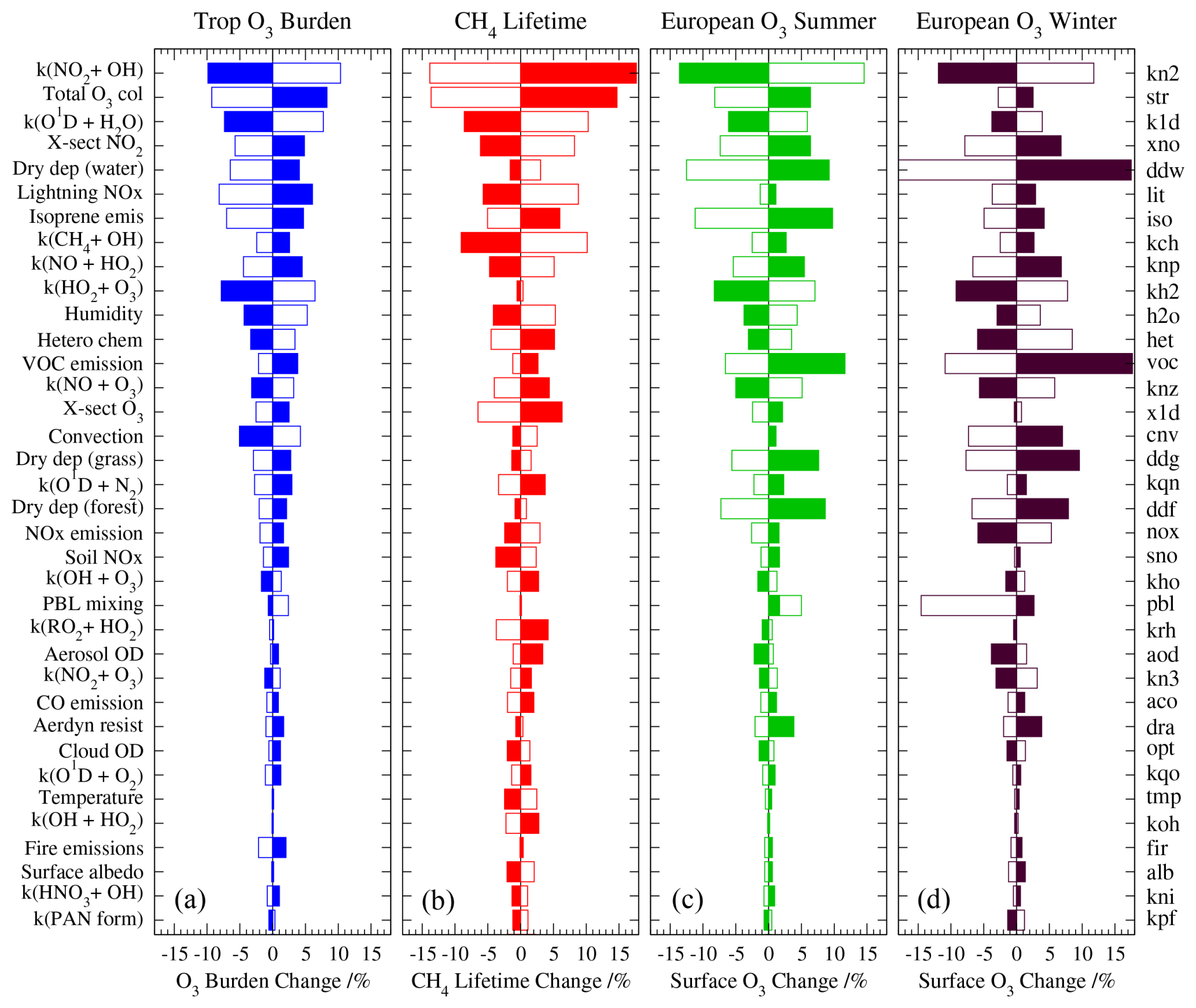
Figure 1 Sensitivity of global tropospheric ozone burden (a), tropospheric methane lifetime (b), and European surface ozone in summer (c) and winter (d) to individual parameters from one-at-a-time studies. Parameters are set to the top and bottom of the uncertainty ranges defined in Table 1; responses at the top of the range at shown in strong colours and at the bottom of the range are shown in outline.

3.2 Sensitivity to key processes

We first investigate the sensitivity of tropospheric ozone and oxidant budgets to each parameter independently by performing one-at-a-time simulations with the model at the top and bottom of the 2σ uncertainty range for each parameter using the ranges given in Table 1. We show the impact of each parameter on the annual mean tropospheric ozone burden and methane lifetime in Fig. 1, along with the impact on seasonal mean surface ozone over Europe in summer and winter. We choose the European region (10° W–30° E, 35–65° N) as broadly representative of polluted mid-latitude conditions, and show summer and winter to highlight the contrasting seasonal influences of physical and chemical processes. The model control run has a tropospheric ozone burden of 318 Tg, a methane chemical lifetime of 9.3 years, and European regional mean ozone mixing ratios of 50 and 30 ppb in summer and winter respectively, but we show relative changes in Fig. 1 to permit comparison across these different variables. The absolute impacts of all parameters considered here on these metrics and on a wider range of ozone chemical production, destruction and deposition terms are given in Table S1 in the Supplement.

The parameter with the largest impact on tropospheric ozone and OH is the rate constant for the reaction of NO₂ with OH (labelled kn2). A 2σ uncertainty in this rate constant contributes  ± 10 % uncertainty in the tropospheric ozone burden and  ± 15 % uncertainty in methane lifetime, as well as strongly influencing surface ozone. Previous studies have noted the importance of this reaction; Newsome and Evans (2017) found a 6 % uncertainty in the ozone burden and 10 % uncertainty in OH from a 1σ uncertainty in the rate constant. This highlights the continuing need for high quality lab measurements of reaction kinetics. The effects of the total O₃ column on photolysis rates, which initiate and maintain tropospheric oxidation processes, is also important, as is the rate constant for the reaction of O(¹D) with water vapour, which acts as an important sink of ozone and the major primary source of OH. It is notable that these two parameters have opposing influences on O₃ and OH, while the reaction between NO₂ and OH affects O₃ and OH in the same sense, highlighting the different roles these reactions play in tropospheric oxidation.

The importance of the parameters differs substantially across the metrics considered here. The reaction between HO₂ and O₃, for example, has a strong impact on ozone, but relatively little impact on methane lifetime, despite being a source of OH. Lightning NO emissions strongly affect the tropospheric ozone burden and methane lifetime, but have relatively little effect on surface ozone in Europe. In contrast, dry deposition parameters have a strong impact on surface ozone, as expected, but a moderate impact on the tropospheric ozone burden and relatively little effect on methane lifetime. The contrasting magnitude and sign of the impacts over different metrics highlights the possibility of applying observational constraints over a range of different metrics to provide insight into the specific parameters responsible for the discrepancy between model simulations and observations, informing model development and reducing model uncertainty.

Most parameters considered here show broadly linear behaviour in their effects, with impacts from increased or decreased values at similar magnitudes and with opposite sign (although we note that some asymmetry may be expected where we have assumed a logarithmic uncertainty range). However, this is not the case for all parameters, and some show distinctly non-linear behaviour. The boundary layer mixing rate (pbl) is a good example, and has a much larger effect on surface ozone in wintertime when mixing is reduced than when it is increased. This reflects the deposition and chemical titration of ozone by NO in polluted environments when air is trapped close to the surface. Interestingly, surface ozone in summertime increases under both reduced and enhanced mixing, reflecting the competition between photochemistry, deposition and vertical mixing processes in governing surface mixing ratios. Most parameters affect surface ozone in summer and winter in a broadly similar manner. However, dry deposition to water, ice and bare ground (ddw) has a substantially larger impact in winter, and becomes the dominant parameter in this season. The sensitivity to anthropogenic VOC emissions (voc) also increases, partly reflecting the reduced availability of isoprene from biogenic sources in winter. The effect of anthropogenic NO_x emissions (nox) changes sign; increased emissions in summertime lead to enhanced ozone production, while increases in winter, when photochemistry is much slower, lead to enhanced titration and to a lower ozone abundance.

To make a full global sensitivity analysis feasible, we reduce the number of parameters considered by discarding those that have little impact on the tropospheric ozone burden, methane lifetime or surface ozone. The 60 parameters are ranked based on a weighted mean of their relative contributions to uncertainty across these three metrics, and the ranking is reflected in the ordering shown in Fig. 1. Using this approach we identify 36 parameters that make a root mean square contribution to the total uncertainty across the metrics of at least 1 %, and these parameters contribute 99 % of the combined uncertainty over all 60 parameters considered.

4 Global sensitivity analysis

One-at-a-time sensitivity studies provide a good indication of the importance of individual parameters in influencing metrics such as global ozone burden or methane lifetime, but cover only a small fraction of the input parameter space defining the uncertainty across all parameters. Investigating this uncertainty in detail requires a very large number of model runs spanning the full parameter space, and this is not computationally tractable with a complex CTM. We therefore use Gaussian process emulation to emulate the output of the CTM, following standard methods described in previous studies (Lee et al., 2011; Ryan et al., 2018), and apply the emulator to explore the full parameter space. We focus on the 36 parameters with the greatest influence as indicated in Table 1 and use a maximin Latin Hypercube design to select 250 combinations of parameter values sampled uniformly from the 2σ uncertainty ranges that optimally cover the parameter space. We assume a uniform distribution of parameter uncertainty rather than normal/log-normal distribution to obtain a broad estimate of model uncertainty and avoid heavy emphasis on prior values. We include a further 30 combinations of parameters to serve as an independent test of the emulators generated. For each combination of parameters, the CTM is run for the full year of 2001, following an 8-month spin-up period, and emulators are built from the monthly output of the 250 model simulations. We focus initially on emulators for the global ozone burden and methane lifetime, but then expand this to look at monthly mean distributions of ozone at the surface and in the mid-troposphere. Each point in space and time from the model output is emulated independently, and we therefore build 1538 emulators (64 locations × 12 months × 2 altitudes +2 global metrics) to cover the measurements considered here.

The skill of the emulators in representing the full model is evaluated by quantifying how well they reproduce the results of the 30 additional runs on which they were not trained. Overall the emulator performance is good for the ozone burden (r²=0.98, RMSE=5.2 Tg), methane lifetime (r²=0.97, RMSE=0.3 years) and global annual mean ozone at the surface (r²=0.98, RMSE=0.7 ppb) and at 500 hPa (r²=0.99, RMSE=0.8 ppb), see Fig. S1 in the Supplement. About 30 % of the residual error across these metrics arises from just three points that lie close to the edge of the uncertainty range for important parameters. We note that the least well represented of the metrics considered here is the methane lifetime, which is underestimated with the emulator at the longest and shortest lifetimes. However, if emulation is performed in reciprocal space, on methane loss rate, then these points lie much closer to the simulated values and within the 95 % confidence intervals of the emulator, suggesting that this would be a better approach. Overall, our evaluation gives confidence in use of the emulators, while also providing a quantitative indication of the uncertainty involved.

We first use the emulators to perform a global uncertainty analysis for the model tropospheric ozone burden and methane lifetime by using a Monte Carlo approach to sample the full parameter space, drawing one million sets of values sampled uniformly from across the uncertainty range in each parameter. We find a mean ozone burden of 316.8 ± 39.9 Tg and a methane lifetime of 9.66 years ± 1.77 years. The ozone burden is close to that from the control run, and similar to that from our earlier study, 316 ± 23 Tg (Wild et al., 2020), although the 1σ uncertainty is larger, reflecting the much wider range of parameters considered here. The uncertainty, about 13 %, is slightly larger than the 10 % estimated from chemical parameters alone by Newsome and Evans (2017), reflecting the broader range of processes included, and it encompasses the 10 % intermodel spread seen in recent model intercomparison studies (Young et al., 2018). The mean methane lifetime is slightly longer than in the model control run, but we note again that lifetime is a reciprocal measure, inversely proportional to loss rate, and we find a harmonic mean CH₄ lifetime of 9.32 years, very close to that in the control run. The 1σ uncertainty of 18 % is again slightly larger than the 16 % estimated by Newsome and Evans (2017), and encompasses the intermodel spread of 10 % found in the ACCMIP intercomparison studies (Voulgarakis et al., 2013), although we note that all models used the same anthropogenic emissions in the latter studies.

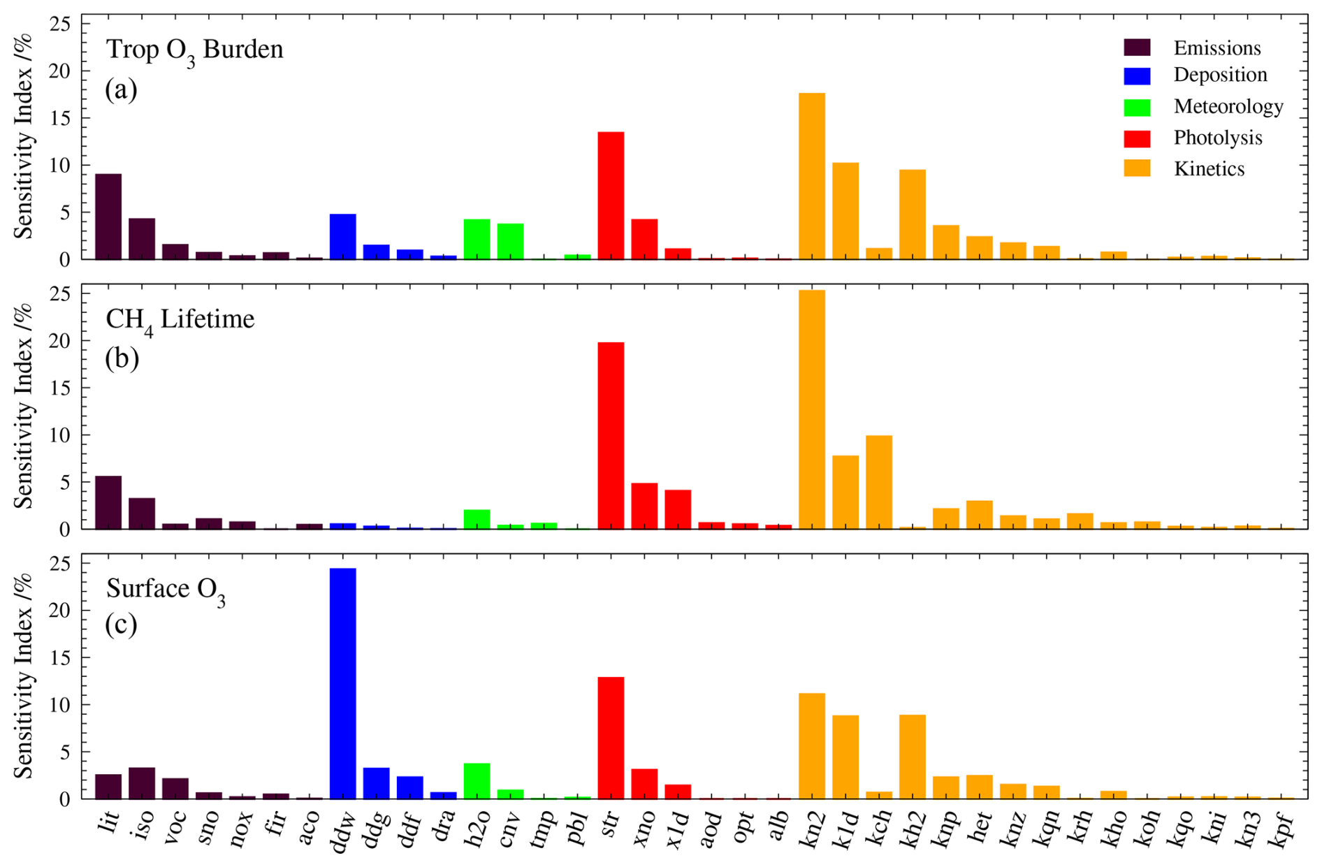
Figure 2 Sensitivity indices for each parameter for annual mean (a) tropospheric ozone burden, (b) tropospheric methane lifetime and (c) global mean surface ozone. The sensitivity index quantifies the contribution of uncertainty in a parameter to the overall uncertainty in a specific metric. Parameters are grouped and ranked by type of process (different colours) to aid comparison, and full definitions are given in Table 1.

The contribution of the uncertainty in each parameter to the overall uncertainty in each metric can be derived using variance-based decomposition. We calculate first-order sensitivity indices using the extended FAST approach developed by Saltelli et al. (1999) as described in Ryan et al. (2018), apportioning the variance in the model outputs to the different sources of variation in the model inputs. Both linear and logarithmic parameter scalings are accommodated by transforming the input ranges to a linear 0 to 1 scale for each parameter. The interaction between parameters can also be quantified through this approach, but these are relatively small for the metrics we consider here and we choose to neglect them for simplicity. The sensitivity indices for each parameter for the tropospheric ozone burden, methane lifetime, and global mean surface ozone are shown in Fig. 2. Uncertainty in the rate constant for NO₂ + OH makes the largest contribution to uncertainty in both the tropospheric ozone burden (18 %) and methane lifetime (25 %), and uncertainty in the rate constant for O(¹D) + H₂O and in stratospheric ozone column also make important contributions. The relative contributions from different parameters are broadly consistent with those derived from the one-at-a-time studies shown in Fig. 1, as expected. On a global average basis, surface ozone is most strongly impacted by deposition to water, bare ground and ice (24 %), reflecting the global dominance of these surface types and the longer lifetime of ozone in more remote environments. However, uncertainties in chemical kinetic parameters also play a substantial role, together accounting for 38 % of the uncertainty in surface ozone, 49 % in ozone burden, and more than 54 % in methane lifetime. Uncertainty in emissions makes a relatively modest contribution overall, ranging from 9 % for surface ozone to 17 % for the tropospheric ozone burden.

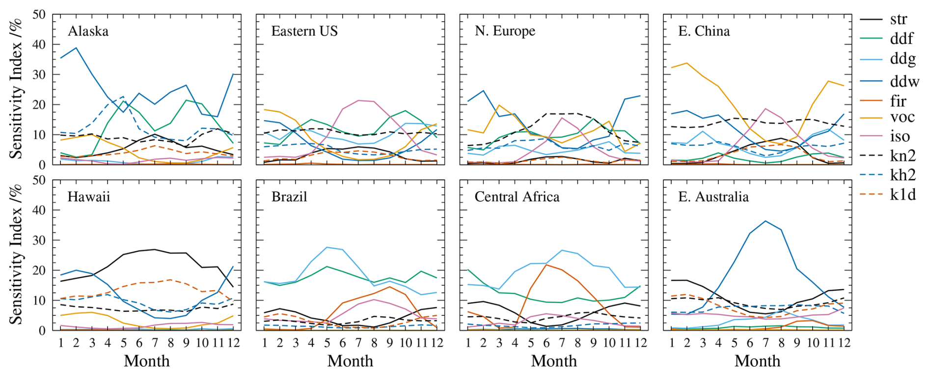
Figure 3 Sensitivity indices (%) for the dominant parameters affecting surface ozone at selected locations around the world. A high value of the sensitivity index for a given month indicates that surface ozone is particularly sensitive to uncertainty in the corresponding process at that time. Parameters shown include the stratospheric O₃ column (str), dry deposition to forest, grassland and water/bare ground (ddf, ddg, ddw), emissions from fires (fir) and anthropogenic and biogenic sources of VOC (voc, iso) and chemical rate constants for NO₂ + OH (kn2), HO₂ + O₃ (kh2) and O(¹D) + H₂O (k1d).

Sensitivity indices for the parameters dominating the uncertainty in surface ozone are shown for a range of different locations in Fig. 3. This highlights how the processes governing surface ozone in the model vary substantially with location and season. At mid and high latitudes in wintertime surface ozone is most sensitive to dry deposition to water, bare ground or ice (ddw), and while this process is dominant in remote and marine regions, it remains important over mid-latitude continental regions. In clean tropical regions, sensitivity to the stratospheric ozone column is important, highlighting the key role that photochemical processes play in governing ozone mixing ratios in these locations. Polluted northern mid-latitude continental regions show a substantial sensitivity to anthropogenic VOC emissions in wintertime, as this governs ozone production in NOx-rich environments, and this is particularly evident over Eastern China, and to a lesser extent over the US and Europe. During the summertime, isoprene emissions play a larger role, notably in the southeastern US. Over Brazil, deposition to the Amazon rainforest and Cerrado play the dominant role, but there are substantial seasonal contributions from isoprene emissions and biomass burning. The influences over central Africa are similar, with a particularly strong seasonal role for fire emissions. Over Australia, dry deposition to bare ground and ocean dominates in Austral winter, and photochemical parameters dominate in summertime. There is sensitivity to the most important photochemical reaction rates, NO₂ + OH, HO₂ + O₃ and O(¹D) + H₂O (kn2, kh2, and k1d respectively) at all locations globally, particularly in summertime, and while these parameters rarely dominate, together they contribute about 28 % of the total sensitivity, highlighting their importance on a global scale. It is notable from the examples shown in Fig. 3 that O(¹D) + H₂O dominates in humid tropical regions where sunlight is strong, NO₂ + OH dominates in NOx-rich continental mid-latitudes, and HO₂ + O₃ dominates under clean conditions at high latitudes. In the free troposphere, the difference between locations is smaller and the seasonality is substantially less (see Fig. S2). The contribution of surface processes such as emissions and deposition is less, as expected, and photochemical processes play a larger role. At 500 hPa, the reaction rate for NO₂ + OH dominates throughout the year at most locations, typically contributing 15 %–20 % of the total uncertainty.

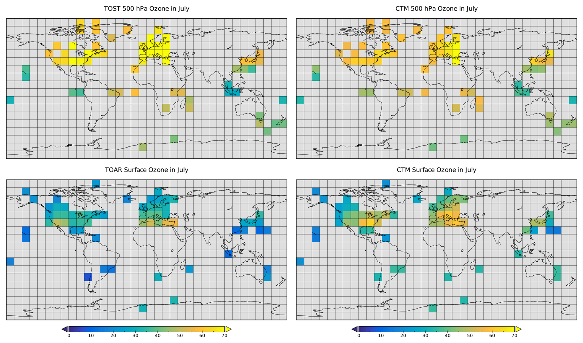
Figure 4 Locations of observations used to constrain the model for mid-tropospheric ozone at 500 hPa (upper panels) and surface ozone (lower panels). Ozone mixing ratios (in ppb) in July at 10° × 10° resolution are shown from the TOST and TOAR observed climatologies (left panels) and the model control run (right panels).

5 Model constraint

The differing magnitude and seasonality of the process contributions at different locations highlights the potential to use observations to constrain overall model uncertainty, as each location has a unique fingerprint of contributions and can provide independent information about the governing processes. Constraining model parameters is a first step towards calibrating the model against observations, and we explore here the feasibility of doing this for ozone. We apply globally-distributed measurements of ozone at the surface from the TOAR dataset and in the mid-troposphere at 500 hPa from the TOST ozonesonde product, see Fig. 4. Both datasets have a bias towards continental locations in the Northern Hemisphere, but we attempt to balance this through site selection to maximise the diversity of environments sampled and their geographical spread.

We calibrate the model by first substituting it with Gaussian process emulators that predict monthly mean ozone at each observation point (12 months at 64 locations at each altitude) and then finding values for each parameter within the defined uncertainty range that minimise the overall difference between the modelled and observed ozone across these points. The calibration algorithm used in this study is described in detail in previous work (Ryan and Wild, 2021), but we provide a brief overview here. We use Gibbs sampling, a Markov Chain Monte Carlo algorithm well suited to Bayesian inference. The algorithm operates by moving around the multi-dimensional parameter space in a series of steps. An initial parameter state vector is selected randomly, and the emulator is evaluated with this parameter set. A new step is made by perturbing the parameters by a small amount, ensuring that the new parameter set is consistent with the prior probability distribution, for which we assume a uniform distribution across the uncertainty ranges defined in Table 1, and then evaluating this new set using the emulator. The new step is accepted if the mismatch between the proposed values and the observations is less than the mismatch from the previous step. The mismatch is specified using a likelihood function, details of which are given in Ryan and Wild (2021). A new perturbed parameter set is then generated and the process is repeated for at least 6000 iterations, when convergence to the posterior distribution is achieved. The first 1000 iterations are discarded as burn-in, and the accepted parameter sets from the remaining iterations are then sampled every fifth iteration to minimize autocorrelation. This process is repeated three times to generate three independent chains, and the resulting 3000 samples are combined to produce the posterior distribution.

We calibrate the model against all four sets of metrics (monthly mean observed surface ozone at 64 locations, monthly mean observed 500 hPa ozone at 64 locations, the global ozone burden and the methane lifetime), weighting these equally. We also explore the effect of calibrating against different combinations of metrics. The global metrics provide insufficient information alone to provide a reliable constraint on the parameters, as agreement with these two values can be achieved through a broad range of different parameter combinations. The global ozone burden provides little additional information to the 500 hPa ozone, as these metrics are closely related. However, constraining with surface ozone alone gives substantially different results from use of all four metrics, and we discuss this further below.

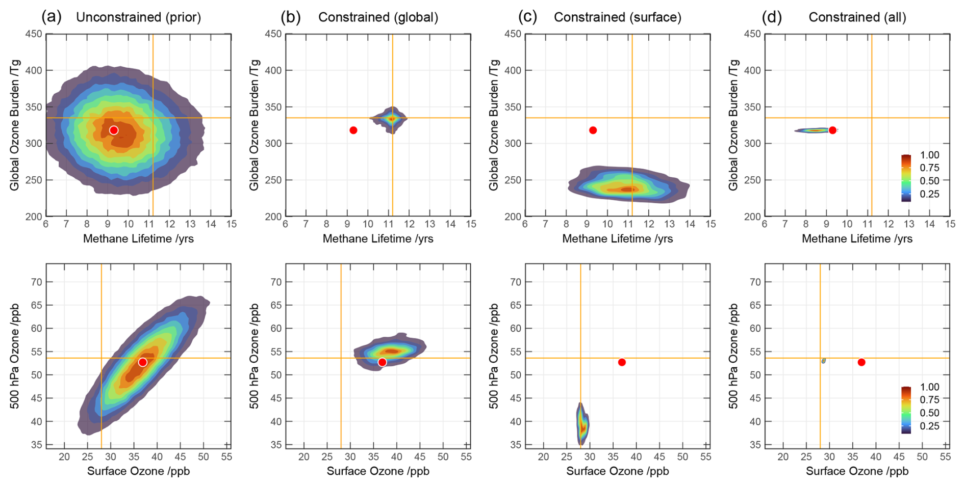
Figure 5 Two-dimensional normalised probability distributions for the global metrics (ozone burden and methane lifetime, upper row) and ozone metrics (500 hPa and surface mixing ratios, lower row) showing the effects of calibration on the emulated quantities. Panels show the unconstrained prior distributions (a), along with distributions following constraint with global metrics only (b), with surface ozone only (c) and with all metrics (d). Mean observation-based values are shown with orange lines, and the model control run is shown with a red circle.

The effects of calibration on the four metrics are shown as two-dimensional probability distributions in Fig. 5. The unconstrained (prior) probability distributions of the global metrics are large and uncorrelated, encompassing the observation-based estimates, and the peak in the distribution lies close to the results from the standard model control run, which underestimates ozone burden and methane lifetime. For the surface and 500 hPa ozone metrics, the distributions are correlated reflecting the interdependence of ozone at the two altitudes. The prior distributions independently span the observation-based estimates, but the joint distribution is not broad enough to encompass the combined estimates. This suggests a structural weakness or missing process in the model, as it is unable to match the large observed difference in mean ozone between the surface and 500 hPa of 25.6 ppb, reaching only 15.8 ± 3.6 ppb even across the full range of process uncertainty considered here. Given that this vertical gradient in O₃ cannot be reproduced even with the large uncertainty range adopted here for dry deposition processes, it is likely that the discrepancy arises from the relatively coarse resolution of the model. The model is unable to represent the range of clean and polluted environments that may lie within a grid box. In addition, the lowest model layer is nearly 100 m deep, and this precludes representation of sub-grid near-surface ozone, particularly when turbulent mixing is weak. This constitutes a structural uncertainty in the model that we are not able to address here directly. Our finding highlights the value of uncertainty analysis in revealing model weaknesses and missing processes, as other studies have noted (Regayre et al., 2023).

Calibration with the two global metrics alone generates a posterior distribution with a strong peak centred on the observed estimates, see Fig. 5, demonstrating the effectiveness of this approach to constraint. The ozone mixing ratios at the surface and at 500 hPa remain relatively poorly constrained, although the probability distributions of both variables are narrowed substantially. The mean ozone at 500 hPa lies close to but slightly higher than that observed, reflecting the small increase in the tropospheric ozone burden, but mean surface ozone remains substantially overestimated by more than 10 ppb on average. A summary of the performance for each metric is given in Table 2.

Table 2 Impact of constraints on representation of observation-based metrics, presented as mean bias (all metrics) and root mean squared error (ozone metrics: monthly mean mixing ratios over 64 locations)

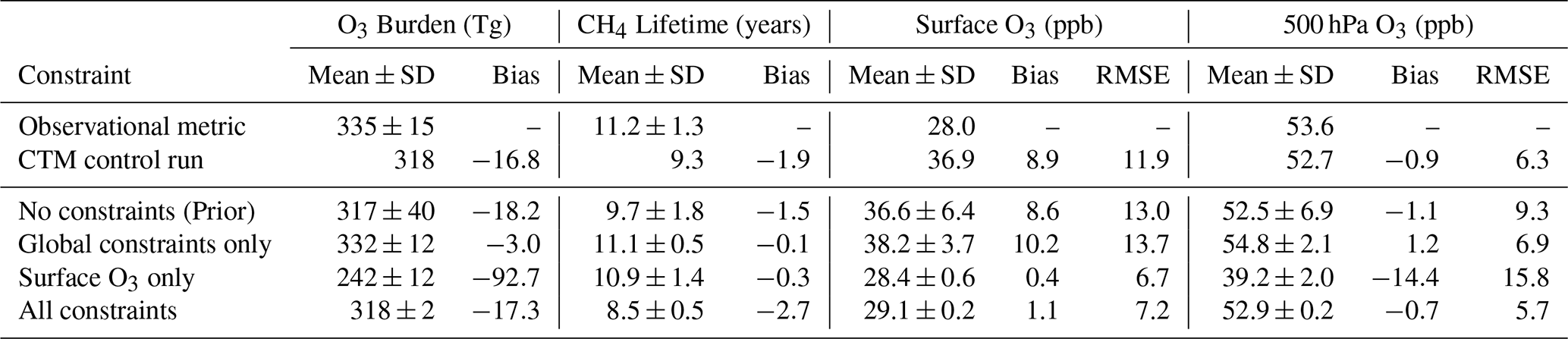
Calibration with observed monthly surface ozone across the 64 locations brings surface ozone into close agreement with the observations, as expected. However, these constraints greatly reduce ozone throughout the troposphere, and the mean predicted ozone at 500 hPa is 39 ppb, about 14 ppb less than observed values. The global mean burden is reduced to an unrealistic value of 242 Tg, about 90 Tg lower than the observation-based estimate. Interestingly, while the methane lifetime is not well constrained, spanning 8–14 years, the mean lifetime is 10.9 years, relatively close to the observation-based estimate. Failure to match the tropospheric ozone burden highlights the importance of applying constraints across a range of different metrics at the same time to reduce the likelihood of matching selected observations for the wrong reasons. We note that the discrepancy between the methane lifetime and ozone burden suggests a second structural error associated with excess OH for a given ozone abundance. This may be accounted for by missing chemical sinks for OH, such as higher VOCs or halogen chemistry that are not represented in the current model configuration.

Calibration using both global metrics and the observed monthly ozone at the surface and 500 hPa provides tighter constraints and brings both surface and 500 hPa ozone into close agreement with the observations, within 1.0 ppb. However, this is only achieved with an underestimate in ozone burden of 17 Tg and a methane lifetime of 8.5 years, somewhat shorter than in the control run. The inability to constrain all metrics simultaneously is a consequence of the prior probability distribution not fully encompassing the observations, and again highlights the structural errors we have identified.

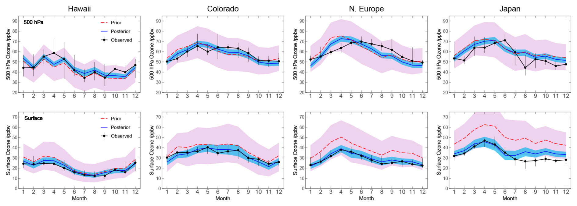
Figure 6 Seasonal cycles of monthly mean ozone (in ppb) at 500 hPa (upper row) and the surface (lower row) at selected locations across the globe. Uncalibrated (prior) simulations and their associated uncertainty (shading represents 95 % confidence intervals, including emulator uncertainty) are shown along with calibrated (posterior) simulations; observations are representative of 2001, and bars show interannual variability over a ±3 year period around this.

While the combined calibration does not improve the model simulation of the global metrics, we show the effect on ozone and its seasonality at selected locations in Fig. 6. Mid-tropospheric ozone and its variations are represented relatively well in the uncalibrated model, but surface ozone is substantially overestimated in more polluted environments, and by as much as 15 ppb in parts of East Asia. The prior probability distribution accommodating all uncertainties considered here encompasses the observed monthly mean mixing ratios at all but one of the locations shown here. The posterior constrained distribution is much narrower and matches the observations more closely, particularly at the surface, but does not fully encompass the observed changes from month to month. This reflects our focus on annual, global parameter uncertainties in this study, which do not account for regional or temporal variations, and are thus not able to fully match month-to-month variations. Despite this, there are improvements in seasonality at many locations that reflect differing changes in the most influential driving processes. For example, while the spring peak in mid-tropospheric ozone over Europe remains overestimated, mixing ratios are reduced in spring and increased in summer, bringing the modelled seasonality into closer agreement with observations. This is also seen in the reduction in root mean squared error across monthly ozone shown in Table 2. Further improvement in capturing ozone seasonality would require consideration of the temporal and spatial uncertainties associated with key processes such as deposition, emissions and transport, and this would be a valuable goal for additional parameter uncertainty studies.

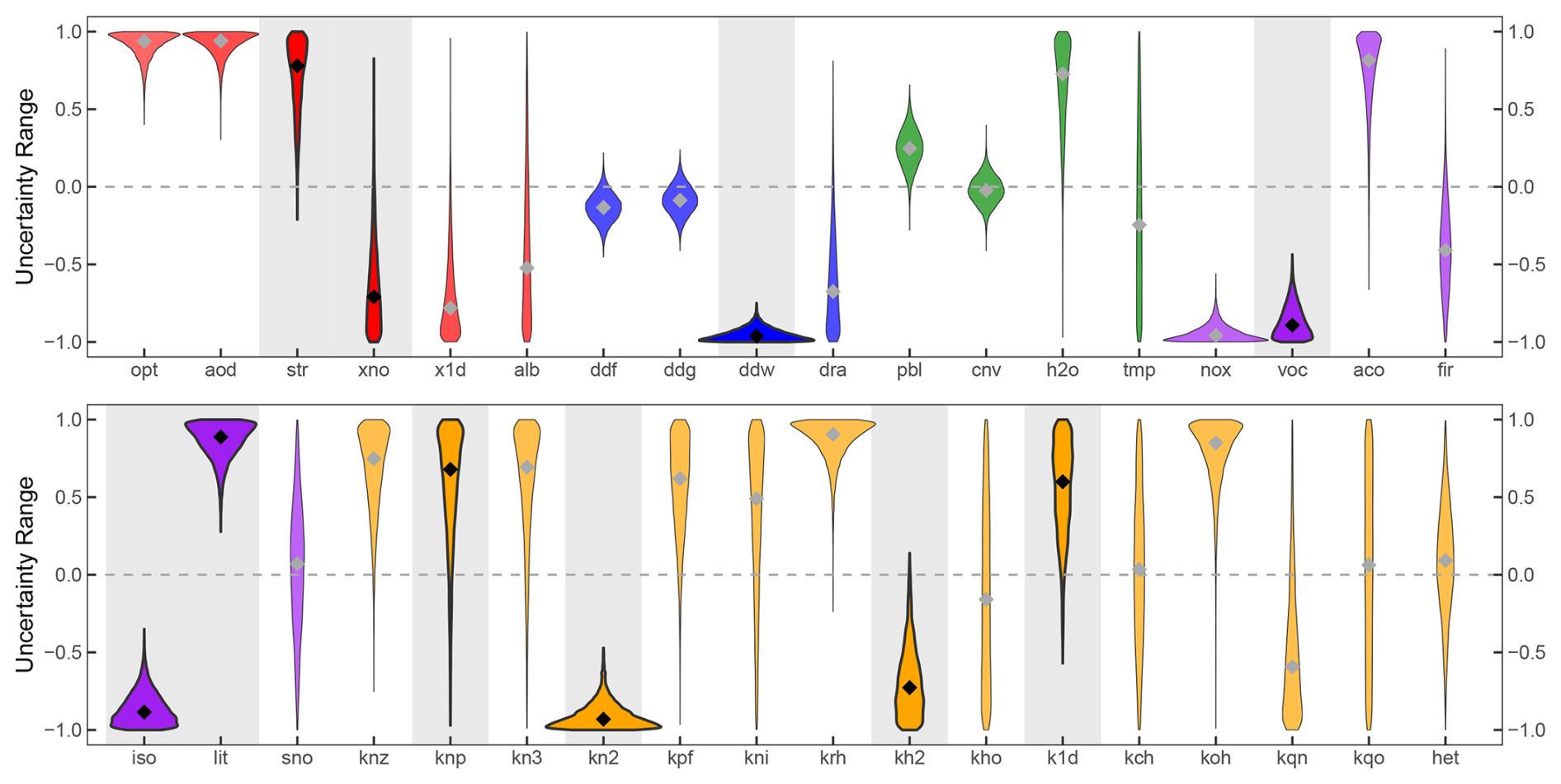
Figure 7 Probability distributions for each parameter following calibration; mean values are shown as points. The full uncertainty range for each parameter is normalised to ±1.0, where 0.0 represents the standard unperturbed parameter value used in the control run, and positive values indicate posterior parameter values that are larger than in the control run. The prior distribution of uncertainty in each parameter is assumed uniform, and where the parameter has little influence or is unconstrained the posterior distribution remains relatively uniform. Parameters are coloured by process type following the same scheme as Fig. 2, and the 10 parameters with the greatest influence are highlighted in stronger colours on a shaded background.

6 Process constraint

The calibration process reveals the parameter values required to meet the observational constraints. Figure 7 shows the posterior parameter distributions following constraint with all metrics. We consider all sets of parameter values meeting these constraints, not simply the optimal set, as there may be a range of equally plausible sets between which we are not able to distinguish within the observational uncertainty. Nevertheless, we find consistent constraints on the most important parameters that provide valuable information on specific processes and guide model improvement. The 10 parameters with the greatest influence are shown in stronger colours; these each contribute more than 4 % of the total uncertainty, and together account for 78 %. Parameters with little influence are typically poorly constrained, as expected. In light of the known biases in the standard control run, the constrained parameter distributions are generally intuitive, with values that act to reduce surface ozone, maintain mid-tropospheric ozone, and reduce chemical reactivity through limiting OH. The most important effect is reduction in the surface resistance for deposition to water and bare ground, which enhances deposition to unvegetated surfaces and reduces surface ozone across the globe. This is reinforced by reductions in emissions of isoprene and VOC, which reduce continental surface O₃ production. Interestingly, the constraints suggest that lightning NO emissions should be larger, increasing tropospheric OH; however, coupled with the reduction in surface NO and VOC emissions, this provides an effective means of enhancing the gradient between surface and mid-tropospheric O₃, which is underestimated in the model. Photochemical parameters are also important and reduced formation of O₃ and OH is supported through larger O₃ columns and smaller NO₂ cross-sections. Higher cloud and aerosol optical depths reduce chemical activity close to the surface and enhance it in the mid troposphere, supporting a stronger vertical gradient in O₃. The reaction rate for O(¹D) + H₂O is enhanced, which reduces ozone but increases OH. However, the reaction rate for NO₂ + OH is reduced, and for NO + HO₂ is enhanced, and these both increase ozone and OH. These changes lead to changes in the distribution of O₃ and OH as well as in their magnitude, reflecting the complex interaction between chemical and meteorological processes across the uncertainty space explored here.

To test the effectiveness of these process constraints for model calibration, we select the 12 parameter sets with the lowest overall bias and run the CTM with these combinations. The results from these 12 independent runs lie close together, despite differing sets of parameter values, and they match surface O₃ well, with the mean model bias reduced to 0.1 ppb (see Figs. S3 and S4). However, while the methane lifetime is improved (9.8 years vs. 9.3 years in the control run), the tropospheric O₃ burden is degraded (298 Tg vs. 318 Tg). It is notable that the bias in the ozone burden is larger than predicted by the emulator, and that the methane lifetime is improved rather than degraded. These differences highlight the increased uncertainty in the emulators at the boundaries of the parameter space explored here. This could be addressed by performing a second perturbed parameter ensemble that targeted this part of the parameter space to refine the emulators in this region of interest.

While the constraints on key parameters are generally intuitive and readily explainable, it is important not to over-interpret their significance given that the joint constraint imposed by the surface and 500 hPa ozone metrics lies outside the uncertainty space considered in these studies. The posterior distributions for some of the key parameters lie at the extremes of the specified uncertainty ranges, far from the prior values, as a consequence of attempting to fit observations outside the uncertainty space, compensating for structural errors. The cause of these structural errors needs to be addressed before this approach can be used to generate meaningful constraints on parameter distributions that would allow reliable calibration.

7 Addressing structural errors

An inability to match all observation-based metrics at the same time indicates the presence of additional uncertainties not fully considered in this study. The uncertainty ranges applied here are intentionally relatively large, and it is unlikely that parameters fall outside these ranges. However, uncertainties in meteorological processes such as advection cannot be addressed easily in an offline framework, and uncertainties in the spatial and temporal variation of emission and deposition processes could not be fully explored. The model may be missing key chemical or physical processes, and may misrepresent processes occurring on physical scales much smaller than the model grid scale. These model structural errors present a substantial challenge to address, and further studies are needed implementing alternative process representations and exploring the impact of chemical or physical processes currently neglected. However, our exploration of observation-based constraints highlights two clear issues for the model: a tendency to overestimate surface ozone, reflecting an inability to resolve near-surface processes, and an imbalance between ozone and OH that suggests weaknesses in model photochemistry. We investigate here how addressing these errors might affect the results of calibration and the diagnosed constraints on the governing processes.

Overestimation of near-surface ozone is a common characteristic of global-scale chemistry-transport models, typically attributed to coarse resolution or to biases in emissions, and has been noted in many previous studies (e.g. Wild and Prather, 2006; Young et al., 2018; Lacima et al., 2023). We take two different approaches to address this bias in the current study. Firstly, we make use of the sub-gridscale information carried as a component of the second-order moment advection scheme used in the model (Prather, 1986), and diagnose the ozone in the lowest third of the surface grid-box, representing a layer about 30 m thick near the surface. The ozone in this layer is about 2 % less than that over the full depth of the lowest model level on a global annual basis, with the largest differences (20 %) over tropical forests and small differences (<1 %) over the ocean. Secondly, we consider how surface abundances are diagnosed in the model. Diagnostics are typically generated at the end of a model time step following a sequence of time-split processes that include emissions, deposition, chemistry and transport. Surface ozone diagnosed following deposition averages 4 % less than that diagnosed following chemistry and transport, with the largest differences (30 %) over continental regions in the tropics and the smallest impacts over the ocean (2 %). For convenience here we combine these two different aspects and take the average of the sub-grid surface ozone before and after dry deposition. This allows diagnosis of near-surface ozone without biasing the values too heavily to deposition processes, and gives an annual mean reduction in surface ozone across the sites considered here of about 11 %. This reduces the mean bias in the control run from 8.9 to 5.5 ppb.

To investigate the influence of missing chemistry, we explore the effects of including halogen chemistry using recent simulations incorporating iodine chemistry. Iodine is believed to account for a large proportion of halogen-related ozone loss, and we find that the tropospheric ozone burden is reduced by about 7.5 %, comparable to reductions of 6 %–10 % found in other studies (Pound et al., 2023; Sherwen et al., 2016), and the methane lifetime is increased by about 1 %. Global surface ozone is reduced by 11 %, with largest reductions over the tropical oceans (25 %), close to iodine sources, and small reductions (5 %) over the continents. As a separate adjustment, we add the recently-identified effects of including water vapour absorption in the calculation of photolysis rates (Prather and Zhu, 2024), which increases the methane lifetime by 4 % and the ozone burden by 2 % in this model.

While it would be valuable to rerun the full perturbed parameter ensemble including these processes, this would be computationally prohibitive, so we estimate the impact by scaling results from the existing ensemble of runs by spatially and temporally-dependent factors derived from the above results. The sub-gridscale treatment affects only the surface mixing ratios, with the largest effects over the continents, while the inclusion of the chemical changes affects all of the metrics, with the largest effects over the surface ocean. Inclusion of these factors increases the CH₄ lifetime from 9.3 to 9.8 years, but reduces the global burden from 318 to 301 Tg; annual mean ozone over the 64 surface locations drops from 36.9 to 30.3 ppb, and annual mean ozone at 500 hPa drops from 52.7 to 49.4 ppb. The modelled prior joint probability distribution of mean surface and 500 hPa ozone now incorporates the observation-based estimates (see Fig. S5) indicating that structural errors hindering calibration have been at least partly addressed. We then repeat the calibration procedure to investigate the constraints this provides on key governing processes.

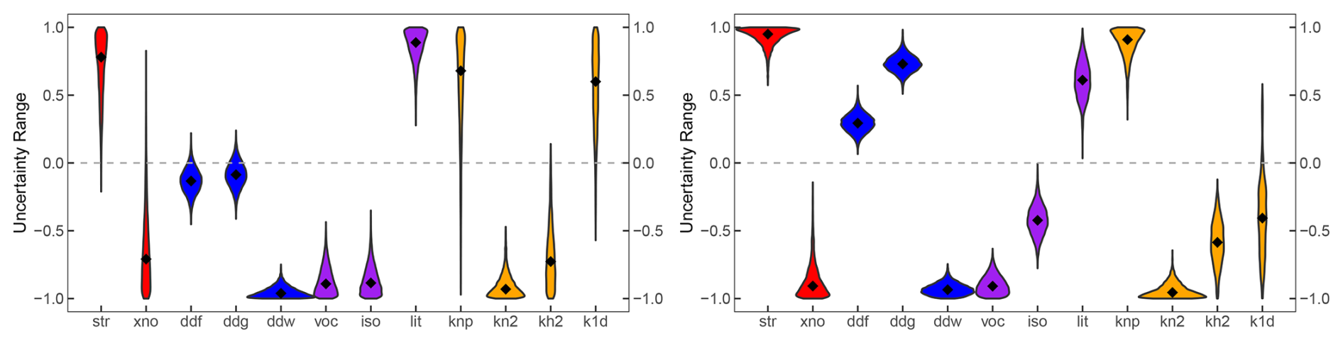
Figure 8 Probability distributions for the most influential parameters following calibration of the standard model (left, taken from Fig. 7) and from the model corrected for structural errors (right). Parameters shown include the stratospheric O₃ column (str), absorption cross-section of NO₂ (xno), dry deposition to forest, grassland and water/bare ground (ddf, ddg, ddw), emissions of anthropogenic VOC, biogenic isoprene and lightning NO (voc, iso, lit) and chemical rate constants for NO + HO₂ (hnp), NO₂ + OH (kn2), HO₂ + O₃ (kh2) and O(¹D) + H₂O (k1d).

Calibration brings the corrected model results into better agreement with the observations than was possible with the uncorrected model, with an ozone burden of 324 Tg, a methane lifetime of 11.2 years, a mean surface ozone mixing ratio of 29.2 ppb and 500 hPa mixing ratio of 53.2 ppb. While the methane lifetime now matches the observation-based estimate well, the ozone burden remains about 3 % low, which may reflect the continuing challenge in reconciling the large observed difference between ozone at 500 hPa and at the surface, where ozone is still 1.2 ppb (4 %) too high. The posterior probability distributions for the constrained parameters remain similar to those for the uncorrected model, with some parameters still far from prior estimates, although the ranges are somewhat smaller and fewer parameters lie towards the extremes of their uncertainty ranges, see Fig. 8 (probability distributions for all 36 parameters are shown in Fig. S6). Constraints on photolytic parameters remain consistent with overactive photochemistry, suggesting that the ozone column should be larger and the NO cross-section smaller. Dry deposition to the ocean and bare ground may still be too low, reflecting overestimated ozone abundance over oceanic regions, but deposition may now be too high over continental regions, where ozone mixing ratios have been reduced. This is also reflected in the constraint on isoprene emissions, where the overestimate may be substantially less than suggested in the initial calibration. Interestingly, the constraint on OH formation through the O(¹D) + H₂O reaction changes sign, as OH is no longer overestimated following the adjustments to model chemistry.

The broad similarity in the probability distributions for the most important of the constrained parameters suggests that the outcomes of calibration are reasonably robust, and are not highly sensitive to differences in model configuration. This makes the information provided valuable in guiding model development. Identification of the parameters with most influence has provided a clear focus on the processes that need improvement in the CTM, and these can be addressed through a review of the key emissions and kinetic data used along with refinement of dry deposition processes. The structural errors identified can be addressed through use of higher model resolution, diagnosis of near-surface mixing ratios in place of lowest layer mixing ratios, and extension of the chemistry scheme, particularly inclusion of wider halogen chemistry (currently underway). Following model refinement, the perturbed parameter ensemble should then be repeated with an updated set of parameters and revised uncertainty estimates. Subsequent calibration would benefit from inclusion of a much wider range of observational metrics covering different species from a variety of surface, airborne and satellite platforms. These would provide substantial additional process constraints beyond the limited set explored in this study. However, use of a much larger set of observational constraints would impose a very heavy computational burden on the calibration process, and exploration of more efficient new approaches to calibration is needed to make this computationally tractable. Finally, it would be valuable to repeat these studies with other global models to explore how the results differ. We encourage others in the modelling community to move beyond using observations for model evaluation alone towards applying them for model calibration. Independent calibration provides an important strategy to reduce model biases and address the wide spread of results seen in model intercomparison studies. Consistent constraint of specific processes across a range of models would also provide strong evidence that our scientific understanding of these processes can be improved.

8 Conclusions

In this study we have applied global sensitivity analysis to an atmospheric chemistry-transport model to determine the importance of key processes in governing tropospheric ozone on a global scale, and to quantify how uncertainties in these processes contribute to uncertainty in modelled ozone and OH. This approach has permitted the first direct comparison of uncertainties across a broad range of very different processes in a uniform manner. We find that the largest contributions to uncertainty in both tropospheric ozone and OH arise from photochemical parameters, in particular from the rate constant for the reaction of NO₂ with OH that governs the tropospheric lifetime of NO_x, and from factors controlling photolysis, which initiates tropospheric photochemistry. The strong sensitivity of ozone and tropospheric oxidation to these processes highlights the fundamental importance of laboratory studies of photochemical kinetics and the need for more confident quantification of key reaction rates to reduce uncertainty in tropospheric oxidation. However, we also highlight other major processes of similar importance for the tropospheric ozone burden, including the influence of total ozone column on photolysis rates, the source of NO from lightning, convective lifting of ozone and its precursors, and deposition to the surface. While we expect broadly similar sensitivity to uncertainty in these processes in different models, differences in process treatment are likely to explain much of the diversity in current global model results.

For surface ozone, we find a large sensitivity to deposition processes, as expected, but note that the greatest uncertainty arises from deposition over water and unvegetated surfaces, driven by the global dominance of these surface types and the greater role of deposition in governing surface ozone in remote regions. Uncertainties in emissions of ozone precursors make an important contribution to uncertainty in ozone in polluted continental regions, but on a global scale they are generally less important than photochemical parameters. We highlight the strong seasonal and spatial variation in the contributions of different processes to surface ozone, and note that while this presents a substantial challenge to representing ozone correctly in models, the distinct fingerprint of uncertainty at each location provides a valuable opportunity to improve process representation through observational constraints.

We show how, through the use of emulation, we can calibrate a global model through identification of parameter values that allow improved representation of tropospheric and surface ozone. This calibration allows us to reduce uncertainty in the governing processes through constraining the range of values needed to match observations, informing model development. However, it also allows identification of structural errors and model weaknesses that are not otherwise evident. We show that the vertical gradient between surface and free-tropospheric ozone abundances is substantially underestimated with the CTM, highlighting the need to better resolve near-surface removal and mixing processes in the model. We also show a tendency to overestimate OH abundance and hence tropospheric oxidation which may reflect missing photochemistry in the model associated with radical sinks, higher VOC chemistry or halogen chemistry. Repeating the calibration process after addressing these weaknesses would permit more reliable constraint on other governing processes.

While we have demonstrated the value of Gaussian process emulation in calibrating a chemistry transport model and identifying model weaknesses, further studies are required to provide more robust constraint on key processes. To make calibration computationally tractable we have used pseudo-parameters to scale the effects of major processes, and have neglected the temporal and spatial variability of emissions and deposition processes, for example, that would permit better representation of the seasonality seen in observations. We have also been unable to explore the impact of uncertainty in meteorological transport processes, which are external to our offline model, or in interactions with aerosol, which are not currently represented. However, the results of this study allow prioritization of the processes to target to reduce model uncertainty. Despite the large number of processes contributing to uncertainty in modelled ozone and OH, most of this uncertainty is driven by a limited number of processes in any particular environment, often less than 10. A more tractable approach to model calibration might therefore involve targeting specific processes in key environments, e.g., emissions and rapid photochemistry in urban conditions, or transport and deposition in clean/remote regions, before coupling these components to constrain processes throughout the troposphere.

Our study also highlights the limitations of applying a single suite of observations, such as of surface ozone, to constrain models. Application of a much wider set of observations of ozone and its precursors such as NO_x, NO_y, CO, HCHO and VOCs, from surface, airborne and satellite platforms, would provide distinct and independent information to permit a more robust constraint of process uncertainty. This is likely to uncover further structural errors in the model that will need to be addressed. However, tackling these issues step by step provides an important observation-driven strategy to improve model performance and process understanding and provides a fresh approach to tackling the diversity in model representation of ozone and tropospheric oxidation that has remained stubbornly large over the past two decades.