The sensitivity of smoke aerosol dispersion to smoke injection height and source-strength: a multi-model AeroCom study

The near-source and downwind impacts of smoke aerosols depend on both emitted mass and injection height. This study examines aerosol dispersion sensitivity to these factors using four global models from the AeroCom Phase III Biomass Burning Emission and Injection Height (BBEIH) experiment. Each model performed four simulations: BASE, using burned-area-based BB emissions GFED4.1s with default injection heights; BBIH, using monthly MISR plume injection heights; BBEM, using fire- radiative-power-based BB emission FEERv1.0; and NOBB, excluding BB emissions. The focus is the April 2008 Siberian wildfire event. Aerosol optical depth (AOD) varies across models. In BASE, all models show a steeper AOD decline from the source to downwind regions than satellite data, indicating inadequate long-range transport or excessive aerosol removal in all models. Moreover, near-source, most models overestimate aerosol extinction below 2 km, suggesting injection heights are too low. In BBIH, MISR plume injection heights slightly improve vertical aerosol distribution, but the magnitude is too small. In BBEM, AOD increases significantly near the source due to enhanced BB emissions; however, the downwind AOD remains largely underestimated in both BBIH and BBEM. Notably, CALIOP lidar reveals aerosol layers above 6 km from source to downwind regions – features absent in all model simulations, although a high bias in the gridded CALIOP data makes the evaluation inconclusive. These results suggest that monthly MISR plume injection heights and enhanced BB emissions alone are insufficient to resolve the model–observation discrepancies. Injecting smoke at higher altitudes in Siberia and reducing aerosol wet removal warrant further investigation.

1 Introduction

Smoke aerosols from wildfires can adversely affect air quality and visibility not only near source locations (Konovalov et al., 2011; McCarty et al., 2017) but also in downwind regions hundreds or even thousands of kilometers away during transport. For example, smoke from the Siberian wildfires in Spring 2008 was found as far away as over Japan (e.g., Ikeda and Tanimoto, 2015), the Arctic (Warneke et al., 2009), and Canada (Cottle et al., 2014). Transported smoke can affect the near-source environment, e.g., the concentration of suspended sediment in a lake (Scordo et al., 2021) and can create air quality issues over extended areas (Liu et al., 2015, Xie et al., 2020; Lin et al., 2024). Wildfires can also impact surface albedo, air temperature, the atmospheric radiation field, cloud properties and precipitation (Lu and Sokolik, 2013; Péré et al., 2014; Lee et al., 2022), and even stratospheric temperature and radiative forcing (Stocker et al., 2021; Das et al., 2021).

The impact of smoke aerosols on environments near the source and downwind depends not only on the emitted mass amount (or source strength), but also on factors such as injection height, chemical transformation, removal processes, and transport after emission (Kahn et al., 2008; Paugam et al., 2016; Wilmot et al., 2022). This is especially true for large boreal forest fires that often emit smoke above the planetary boundary layer (PBL) into the free troposphere, and sometimes even into the lower stratosphere, where long-distance transport is more efficient (e.g., Val Martin et al., 2010, 2018; Peterson et al., 2018). Previous studies have demonstrated that biomass burning (BB) emission injection height has a substantial influence on surface-level air quality and on the agreement between model simulations and observations, particularly during intense wildfire events. Numerous modeling studies have shown that adjusting injection heights can significantly alter simulated surface aerosol and trace gas concentrations, thereby affecting air quality assessments, model accuracy, and radiative forcing estimates (e.g., Li et al., 2023; Feng et al., 2024; June et al., 2025). When smoke remains within or near the planetary boundary layer (PBL), it contributes primarily to elevated regional pollution, including increased surface-level particulate matter and ozone concentrations (Kahn et al., 2008; Val Martin et al., 2010; Petrenko et al., 2012). By contrast, smoke injected into the free troposphere is generally transported more efficiently, with reduced surface deposition near-source, enabling long-range and even intercontinental impacts on air quality and visibility (e.g., Sessions et al., 2011; Sofiev et al., 2012). Intercomparison efforts, such as those produced by the AeroCom community, have consistently identified plume-rise representation as a key factor driving variability in simulated aerosol burdens and transport efficiency (Rémy et al., 2017; Zhu et al., 2018). Uncertainty in modeling the vertical smoke aerosol distribution in models has been reported in many studies, and the issue persists (e.g., Koch et al., 2009; Chen et al., 2009; Koffi et al., 2012; Paugam et al., 2016; Vernon et al., 2018; Zhu et al., 2018; Tang et al., 2022; Li et al., 2023).

Current atmospheric models employ a range of approaches for parameterizing smoke injection height, from simple assumptions to physically based schemes. Common approaches include: (1) Prescribed injection heights that vary with altitude and latitude (e.g., Dentener et al., 2006; Matsui, 2017; Matsui and Mahowald, 2017; Horowitz et al., 2020; Xie et al., 2020). (2) Emission placement within the PBL or at a fixed altitude (e.g., Chin et al., 2002; Colarco et al., 2010; Takemura et al., 2005, 2009). (3) Climatological or seasonally averaged satellite-derived heights, e.g., from the Multi-angle Imaging SpectroRadiometer (MISR) and/or Cloud-Aerosol Lidar with Orthogonal Polarization (CALIOP). (4) Daily satellite plume height retrievals, that constrain model emissions using observed vertical profiles (e.g., Val Martin et al., 2010; Rémy et al., 2017; Vernon et al., 2018; Zhu et al., 2018). (5) Dynamic plume-rise models, that simulate plume rise in real time based on fire radiative power, estimated heat flux, burned area, boundary-layer depth, buoyancy, and/or meteorological conditions (e.g., Freitas et al., 2007; Sofiev et al., 2012; Veira et al., 2015a, b; Paugam et al., 2016; Lu et al., 2023). Each of these approaches has advantages and limitations; for example, the climatological schemes (i.e. scheme 1–3) may present statistical conditions and are easier to implement in models, but they will not capture the highly variable nature of fire emission on daily and sub-daily bases, whereas the more dynamic schemes capture event-to-event variability but may be limited by either satellite coverage (scheme 4) or the accuracy of the input data, and they are sensitive to the parameterizations of atmospheric stability structure, entrainment, and turbulence (scheme 5). These different fire injection representations, along with various fire emission estimates, can lead to a wide range in simulated trace gases and aerosol amounts in the atmosphere, their vertical distributions, long-range transport, surface concentrations, and other environmental impact (e.g., Petrenko et al., 2017; Pan et al., 2020; Parrington et al., 2025).

Our project, named Biomass Burning Emission Injection Height (BBEIH), is a part of the international initiative AeroCom Phase-III study (https://aerocom.met.no/experiments/BBEIH/, last access: 16 December 2025). It is designed primarily to assess the impact of the smoke emission vertical profile, while also examining the impact of emission source strength. We address two key questions in this study: (1) How sensitive are simulated near-source and downwind plume characteristics – including vertical aerosol distribution, near-surface concentration, and Aerosol optical depth (AOD) – to the injection height of biomass burning emissions? and (2) To what degree does the choice of biomass burning emission inventory affect smoke dispersion? Unlike previous studies that typically rely on a single model, the novelty of the current work lies in its multi-model comparative analysis of BB plume representations. Specifically, this project consists of two components: (1) BBIH (BB Injection Height), in which we compare the default vertical distribution schemes implemented in each participating model (corresponding to Schemes 1 and 2 described above) with a uniform application of monthly MISR-derived plume heights (Scheme 3) across all models. (2) BBEM (BB Emission Magnitude), in which we compare the model simulations using two emission datasets obtained with different methods: the Global Fire Emissions Database (GFED) that estimates fire emissions using burned area, fuel load, and combustion completeness (Giglio et al., 2013; van der Werf et al., 2017; Randerson et al., 2018), and the Fire Energetics and Emissions Research (FEER) dataset that derives emissions empirically from satellite-observed fire radiative power (FRP) (Ichoku and Ellison, 2014). Our case study focuses on the boreal fire case over Siberia and Kazakhstan in April 2008, which was the largest fire event in Russia during 2000–2008 estimated from MODIS satellite observations in terms of total burned area (Vivchar, 2011). Long-range transport of this Siberia/Kazakhstan smoke was detected over Alaska during the NASA ARCTAS (Arctic Research of the Composition of the Troposphere from Aircraft and Satellites) and NOAA ARCPAC (Aerosol, Radiation, and Cloud Processes affecting Arctic Climate) field campaigns in April 2008, with CO and aerosol concentrations enhanced above background levels by 100 %–300 % (Warneke et al., 2009, 2010).

In the following sections, we describe the AeroCom Phase III BBEIH model experiment in Sect. 2, then present the results in Sect. 3, discuss the results in Sect. 4, and finally, present the conclusions from this study in Sect. 5.

2 Overview of the AeroCom Phase III BBEIH experiment and analysis approach

In this section, we describe the AeroCom BBEIH model experiment, present the two biomass burning emission inventories we used, and describe the satellite products used for model evaluation.

2.1 BBEIH model experiment

Table 1 presents the model framework and the default BB emission vertical distribution schemes in the four models participating in the BBEIH project, i.e., the schemes used in their BASE experiments. The CAM5-ATRAS (or CAM5 in short) and the GFDL-AM4 (or GFDL) models followed the vertical distribution scheme from Dentener et al. (2006), in which the wildfire emissions are distributed over six altitude bins ranging from 0 to 6 km, according to wildland fire location and type. For example, in regions of 50–60° N, where the April 2008 Siberian wildfire event occurred, BB emissions are distributed vertically as follows: 20 % in 0–0.1 km, 20 % from in 0.1–0.5 km, 20 % in 0.5–1 km, 40 % in 1–2 km, and zero for the remaining layers. Note that the vertical fractional distribution is different for latitudes lower than 30° N and higher than 60° N. In the MIROC-SPRINTARS model (or SPRI), the BB emissions are injected between the surface and the altitude having a sigma level equal to 0.74, assuming a homogeneous mixing ratio (∼ the first 13 levels, approximately 3 km in our study region). In the GEOS-i33p2 model (or GEOS), BB emissions are distributed uniformly up to the top of the Planetary Boundary Layer (PBL).

Table 1 List of models and their default BB emission altitudes in Boreal Eurasia (50–60° N).

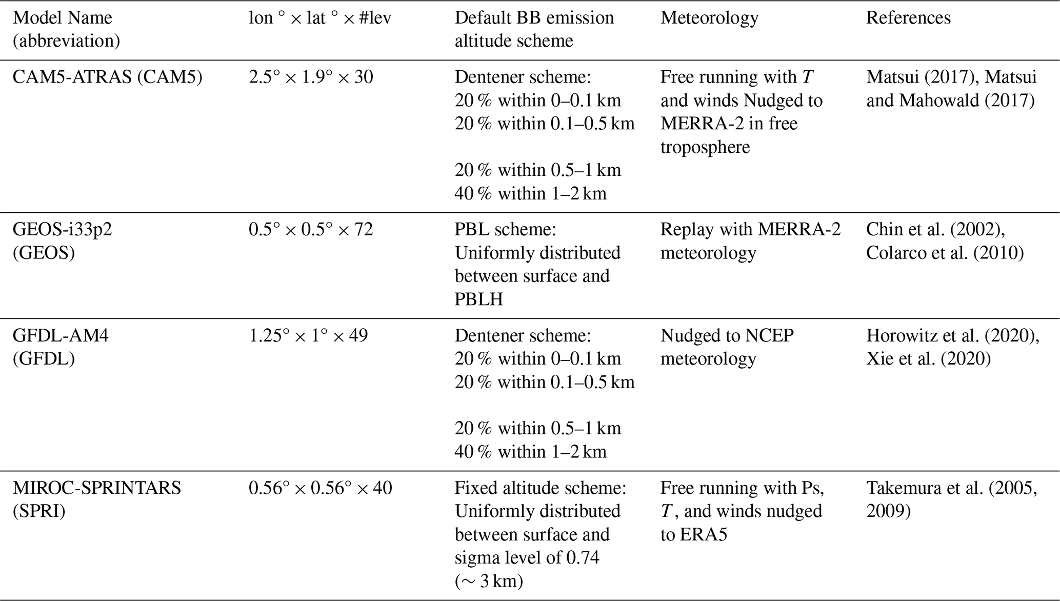
Table 2 List of experiments in the BBEIH project.

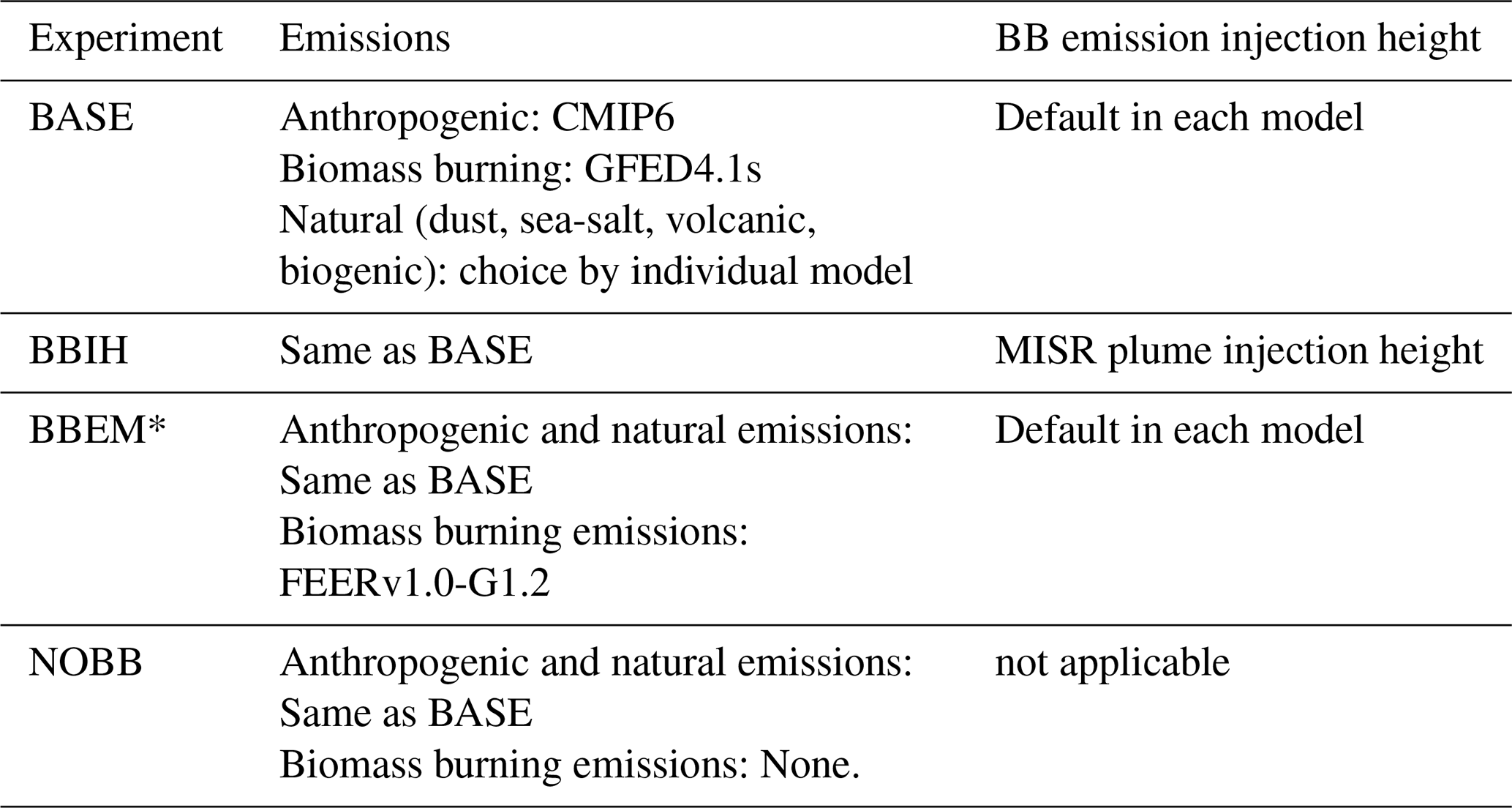
* GFDL does not have this experiment.

The model configurations differ across models. The CAM5-ATRAS model simulates meteorological and chemical fields interactively, including precipitation and wet deposition processes. To better represent realistic meteorological conditions during the simulation period, temperature and wind fields in the free troposphere (pressure <800 hPa) were nudged toward the Modern-Era Retrospective analysis for Research and Applications, Version 2 (MERRA-2) reanalysis. The GEOS model was run in “replay” mode, in which winds, pressure, moisture, and temperature are constrained by the MERRA-2 reanalysis meteorological data (Gelaro et al., 2017). This configuration enables model simulations of actual events, like a traditional offline chemistry transport model (CTM), while also incorporating full model physics, including radiation and moist processes. The GFDL AM4 model is driven by observed sea surface temperatures and sea ice distributions, with horizontal winds nudged toward those from the National Centers for Environmental Prediction (NCEP) reanalysis using a pressure-dependent nudging technique (Lin et al., 2012). Precipitation and temperature are simulated interactively within the model. In MIROC-SPRINTARS, horizontal wind, temperature, and surface pressure are nudged toward the European Centre for Medium-Range Weather Forecasts (ECMWF) Reanalysis v5 (ERA5) data, whereas precipitation is diagnosed using large-scale condensation and cumulus convection schemes, following Watanabe et al. (2011).

Table 2 summarizes the four experiments conducted by each of the four models for the BBEIH project. (1) BASE, i.e., the control run, in which all models used the burned-area-based daily BB emission from the GFED version 4.1s emission inventory (van der Werf et al., 2017), with the model-default biomass burning injection height (Table 1). Other emissions from anthropogenic and natural sources are also included. (2) BBIH is the same as BASE, but the BB emission vertical distribution is constrained by the monthly MISR plume injection height weighting functions (Val Martin et al., 2010, 2018), so the effects of different emission height between BASE and BBIH on aerosol dispersion and vertical distribution can be examined. (3) BBEM, is the same as BASE, but using daily BB emissions from FEER version v1.0-G1.2 (Ichoku and Ellison, 2014), allows us to test model sensitivity to the choice of BB emission inventory. (4) NOBB, is the same as BASE, but with BB emissions turned off, to allow us to isolate the aerosol from biomass burning sources. Accordingly, we derive the BB contribution in each experiment as the difference between the runs from individual experiment (BASE, BBIH, and BBEM) and the NOBB runs.

2.2 BB emissions and injection height

2.2.1 The target regions

Figure 1 highlights the six regions targeted in this study using red boxes. KAZA (over Kazakhstan) and RUS1 (over northeastern Russia) represent the two primary BB source regions. The remaining four regions – RUS2 (over northeastern Russia), RUS3 (further east over northeastern Russia), PAC (over the North Pacific Ocean), and ALA (over Alaska) – are located progressively downwind to the east.

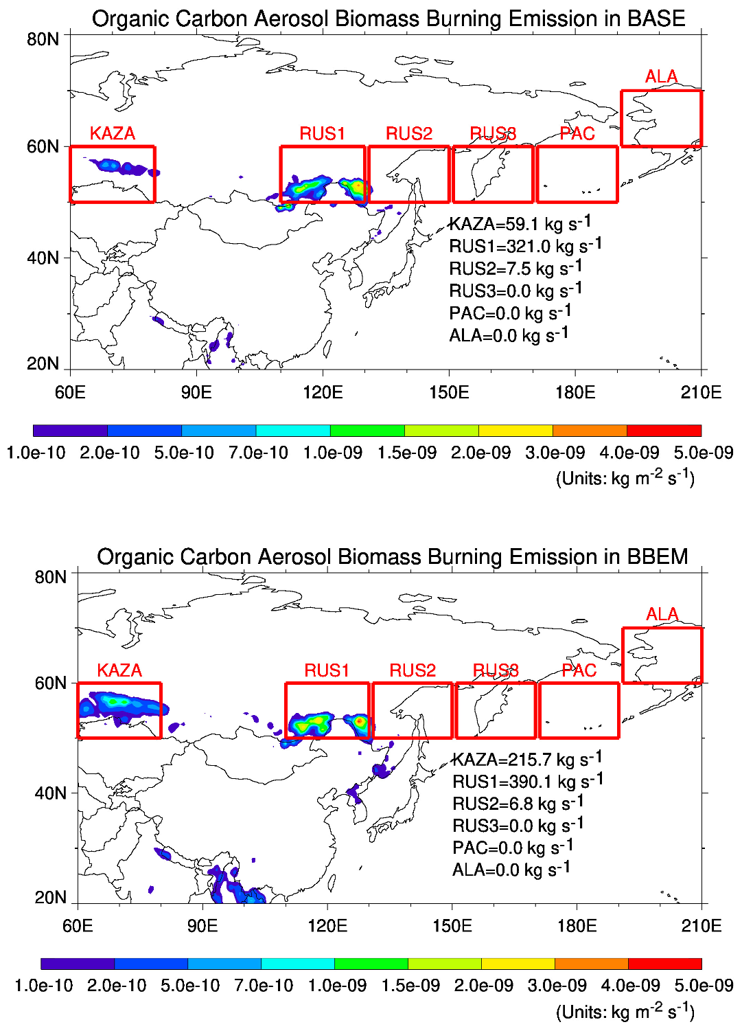
Figure 1 Biomass burning emissions from two inventories. Top: Monthly mean spatial distribution of organic carbon (OC) emissions from biomass burning in April 2008, based on the GFED4.1s inventory (used in the BASE and BBIH runs), in units of $\mathrm{kg}{\mathrm{m}}^{-\mathrm{2}}{\mathrm{s}}^{-\mathrm{1}}$. Bottom: Same as top, but from the FEERv1.0-G1.2 inventory (used in the BBEM run). The six focus regions – KAZA, RUS1, RUS2, RUS3, PAC, and ALA – are outlined and labelled with total emissions.

2.2.2 BB emission inventories: GFED4.1s and FEER1.0

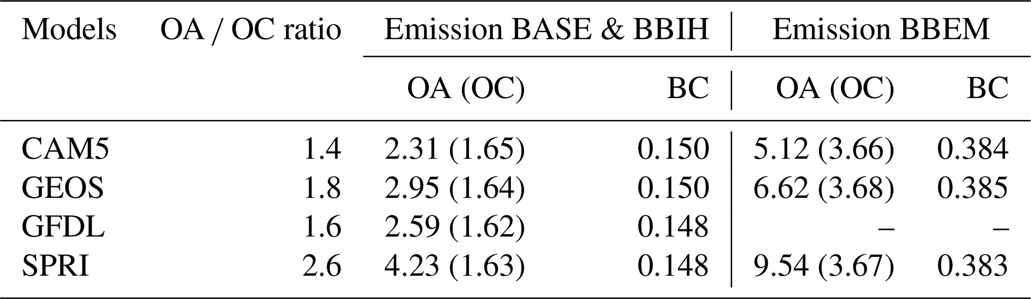
This study employs two BB emission inventories – GFED4.1s (used in the BASE and BBIH run) and FEERv1.0-G1.2 (or FEER1.0, used in the BBEM run) – to assess the sensitivity of aerosol distributions to differences in source strength and spatial allocation. Both GFED4.1s and FEER1.0 provide biomass burning emissions of primary aerosols and aerosol precursor gases such as organic carbon (OC), black carbon (BC), sulfur dioxide (SO₂), nitrogen oxides (NO_x), and ammonia (NH₃), and non-methane volatile organic carbon (NMVOC) gases (van der Werf et al., 2017; Ichoku and Ellison, 2014). The predominant species determining the biomass burning aerosol extinction and AOD is organic aerosol (OA), equal to OC multiplied by an OA $/$ OC ratio. All models participating in the BBEIH include aerosol-related emissions of OC, BC, and SO₂, although the CAM5 and GFDL models include additional NMVOCs, NO_x, and NH₃ aerosol precursor gases. In all cases, OA is the predominant species for BB aerosol mass and AOD.

Figure 1 compares their OC BB emissions for April 2008 from GFED4.1s (top panel) and FEER1.0 (bottom panel). Regional total emissions for each of the six focus regions are also provided in Fig. 1. Emission from FEER1.0 is higher than GFED4.1s by factors of 3.7 and 1.2 in the two major source regions, KAZA and RUS1, respectively. Across both inventories, BB emissions in RUS1, largely driven by forest fires, are substantially higher than in KAZA, where agricultural waste burning dominates. Notably, biomass burning activity in the Siberia–Lake Baikal region peaked in April 2008, exceeding levels observed in other months of the year (see Fig. A1).

GFED4.1s estimates total dry matter consumed by biomass burning by multiplying the MODIS burned area product at 500 m spatial resolution (Giglio et al., 2010) with fuel consumption per unit burned area (van der Werf et al., 2017). The latter is the product of the fuel load per unit area and the combustion completeness. Then, species-specific emissions are derived using an emission factor (EF, in grams of species per kilogram of dry matter burned) from Akagi et al. (2011), supplemented by Andreae and Merlet (2001). GFED4.1s also includes emissions from small fires that were not included in previous versions of GFED (Giglio et al., 2013; Randerson et al., 2012).

In comparison, the FEER1.0 calculates BB emissions based on the satellite-detected FRP from MODIS. More specifically, the BB aerosol emission rate is derived by multiplying ecosystem-specific emission coefficients (Ce) and MODIS FRP data that have been preprocessed and gridded in the GFAS1.2 analysis system (Kaiser et al., 2012). To derive the emission coefficients at pixel level within each grid cell, Ichoku and Ellison (2014) correlate the FRP for multiple cases with the plume AOD and area divided by the advection time (which is estimated from the apparent length of the plume in the MODIS imagery and a wind speed obtained from a reanalysis product). Ce corresponds to the slope of the linear regression fit. Then, the biomass burning emission of a given species is calculated by multiplying the ratio of that species with total particulate matter (TPM), based on the EF (Andreae and Merlet, 2001; updated by Andreae, 2014).

In a previous study (Pan et al., 2020), both GFED and FEER were used, along with four other fire emission inventories, to simulated global AOD with a single model (GEOS). One of the findings relevant to the current study is that FEER estimated higher emissions and produced larger positive AOD biases in April 2008 over the boreal region than GFED. The present study extends this comparison by evaluating GFED and FEER within a consistent multi-model framework. This approach offers a valuable opportunity to identify the drivers of model divergence and to quantify uncertainties in fire emissions and their downstream atmospheric effects. More information on the intercomparison of these two BB inventories can be found at Pan et al. (2020).

Although all models use the same BB emission datasets in the same experiment, the actual emission amount of OA is different among models because different OA $/$ OC ratios are assumed in each model. Table 3 lists the global BB emissions of OA (OC) and BC for April 2008 used in the BASE, BBIH, and BBEM experiments. Although the total emission of OC and BC are the same as in the prescribed emission datasets (small differences due to implementation into the model grid cell), the OA emissions in the models differ by a factor of 1.8, due to the different OA $/$ OC ratios adopted.

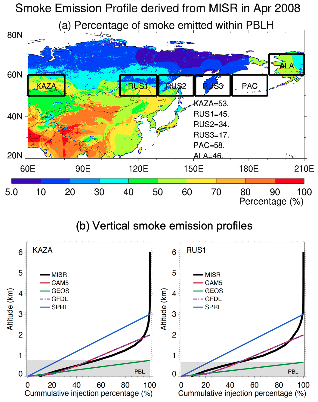
Figure 2 (a) Spatial distribution of the percentage of smoke emitted within the planetary boundary layer (PBL) in April 2008, derived from the MISR- based plume height (units: %), with regional mean values of the six focus regions listed below (over land only). (b) Cumulative vertical smoke emission profiles over KAZA and RUS1, with the black thick curve representing the MISR-based plume height used in the BBIH run and the colored curves representing the model default vertical profiles from the models' BASE runs. The PBL layer is shaded in grey.

Table 3 Global biomass burning emissions of OA and BC for April 2008. Unit: Tg per month.

2.2.3 MISR plume heights for 2008

The MISR-retrieved plume injection height dataset used in BBIH is based on the work of Val Martin et al. (2018; Table S4). This dataset provides regional, monthly AOD-weighted statistical summaries of plume heights, derived using the MISR INteractive eXplorer (MINX) tool (Nelson et al., 2013). The MINX software derives plume heights by assessing the parallax of contrast elements in multi-angle imagery from MISR's nine cameras, which acquire view angles of Earth ranging from 70 forward to 70 aft along the satellite orbit. The product has 1.1 km horizontal resolution and between 250 and 500 m vertical resolution (Nelson et al., 2013). As it takes about 7 min for all nine MISR cameras to image a given location on Earth, the proper motion of plume contrast elements is also obtained and is used to derive plume-level motion vectors, from which wind corrections are made to the geometrically retrieved heights.

Thousands of MISR-observed individual smoke plumes in 2008 were analyzed with the MINX tool, and the resulting vertical profiles were gridded according to six land cover types across seven geographic regions. Although fire detections occurred only at specific locations, the derived profiles were applied across grids sharing the same land cover classification. It is assumed that, within each land cover region, the sampled plume profiles are representative of those in the entire region. This assumption is supported in part by statistical consistency across multiple cases within most land cover types (Val Martin et al., 2018; Junghenn Noyes and Kahn, 2025). The final product is a monthly gridded dataset (longitude, latitude, altitude) with a horizontal resolution of 0.25° and a vertical resolution of 250 m, spanning from the surface up to 6 km in 25 altitude bins. This dataset provides the vertical distribution of near-source biomass burning emissions. For the BBIH simulation, modelers interpolated or re-gridded this dataset to match their model's specific spatial and vertical resolution. The MISR-derived vertical fractions were then multiplied by the corresponding GFED4.1s BB emission amount to place the same fractions of BB emissions at those levels.

Figure 2a reveals the spatial distribution of the percentage of smoke emitted within the PBL in April 2008 (units: %), derived from the MISR-retrieved plume injection height (Val Martin et al., 2018). The numerical values in Fig. 2a represent the area mean percentage of smoke column-abundance concentrated within the PBL in each of the six targeted regions, for April 2008. Figure 2b presents the vertical distribution of smoke emissions for April 2008 over the BB emission source region of KAZA and RUS1. The PBL depth from MERRA-2 is shown in gray shading, with average PBL-top altitudes of approximately 0.77 km in KAZA and 0.68 km in RUS1. MISR-based plume height estimates indicate that only 53 % of smoke in KAZA and 45 % in RUS1 was injected within the PBL, as shown by the black cumulative profiles in Fig. 2b. For comparison, the default vertically cumulative fire emission profiles from the model BASE runs are also shown, with values summarized in Table 1. Among the models, only GEOS places 100 % of fire emissions within the PBL. Both CAM5 and GFDL adopt the vertical distribution scheme from Dentener et al. (2006), resulting in identical vertical injection profiles in their BASE runs; below the PBL top, this scheme allocates a similar fraction of smoke as the MISR-based plume height estimates in KAZA and RUS1. However, this scheme puts no emissions above 2 km, where the MISR-based approach still releases 5 %–10 % of the material. By contrast, SPRI, using the fixed altitude scheme (∼3 km), diverges significantly from the other three models, allocating more smoke above the PBL than any of the other models and the MISR-based results. Overall, nearly all the smoke – close to 100 % – is injected below 3 km in both KAZA and RUS1 across all distribution schemes. This discrepancy is further discussed in Sect. 3.4.

It should be kept in mind that MISR is in a sun-locked, near-polar orbit with a swath-width of about 380 km, so near-global coverage is obtained about once per week – about every 8 d near the equator, and up to every 2 d near the poles (e.g., Diner et al., 1998). Equator crossing occurs at about 10:30 local time, so the typical late-afternoon peak in fire activity is not captured in the MISR observations. Although the MISR-based monthly and regionally averaged plume-height used in the BBIH runs offers a valuable constraint on vertical smoke injection, it does not capture short-term variability in fire intensity or meteorological conditions. Recent work by Junghenn Noyes and Kahn (2025), which analyzed MISR-derived plume heights over Siberia from 2017 to 2021, provides a statistical assessment of plume-height variability in Siberia, stratified by month, ecosystem, and whether plumes were confined to the PBL or entered the free troposphere (FT). They found that approximately 80 % of 117 April fire plumes remained within the PBL. For these PBL-confined plumes, the median height was about 1±0.2 km above sea level, whereas FT plumes reached a median height of about 2±0.5 km. Although these results support the use of monthly mean profiles as a first-order approximation, such monthly and regional averages smooth over high plume events and diurnal variability. For example, although the Val Martin et al. (2018) plume-height included monthly plumes from 2008, the plume injection heights during intense events, such as the strong April 2008 Siberian wildfires examined in this study, may be underestimated.

2.3 Model Evaluation Datasets MODIS, MISR, and CALIOP

We evaluated the simulated monthly AOD at 550 nm wavelength against three satellite datasets: MODIS, MISR, and CALIOP. They each provide spatial and temporal coverage, but with different sampling, across the source and downwind regions, which aligns with the AeroCom Phase III BBEIH experiment design. We computed monthly mean values for each observational dataset and each model within the focus regions, using only the valid data available from each source. Due to the logistical challenges of aligning model output with multiple satellites, each with distinct overpass timing and data gaps, we did not strictly synchronize model sampling with satellite observations. Although this approach introduces some temporal mismatch, it is commonly adopted in multi-model and multi-satellite intercomparison studies to reduce complexity and ensure broader spatial and temporal coverage; it is usually unavoidable in statistically based analyses of this type (e.g., Kim et al., 2019).

MODIS. We used the AOD retrieved from the level 3 monthly MODIS collection 6.1 combined Dark Target (DT) (Remer et al., 2005; Levy et al., 2013) and Deep Blue (DB) (Hsu et al., 2013; Sayer et al., 2014) aerosol algorithm products at one-degree spatial resolution and 550 nm wavelength from both the Terra and Aqua satellites. The DT aerosol algorithm was designed for aerosol retrievals over land (mostly vegetated) and ocean surfaces that are dark from the visible (VIS) to the shortwave infrared (SWIR) parts of the spectrum. The DB algorithm was designed for aerosol retrieval over brighter surfaces such as deserts, using shorter blue wavelengths.

MISR. We used the version 23 monthly level 3 total AOD data at half-degree resolution and 558 nm wavelength from the MISR instrument on board the EOS Terra satellite (Kahn et al., 2010; Witek et al., 2019; Garay et al., 2020; MISR v23, with filename tagged as F15_0032), downloaded from the NASA Langley Atmospheric Sciences Data Center (ASDC) website https://asdc.larc.nasa.gov/project/MISR (last access: 16 December 2025). The MISR product takes advantage of the nine view-angles acquired, ranging from 70° aft, through nadir, to 70° forward along the satellite orbit, at each of four wavelengths centered at 446, 558, 672, and 867 nm (Diner et al., 1998), to derive constraints on particle size, shape, and light-absorption along with AOD (Martonchik et al., 2009; Kahn and Gaitley, 2015).

CALIOP. CALIOP is a two-wavelength backscatter lidar on board the Cloud-Aerosol Lidar and Infrared Pathfinder Satellite Observation (CALIPSO) satellite that has daily equator crossing times of about 13:30 and 01:30 and a 16 d repeating cycle. CALIOP measures directly the aerosol backscatter vertical profiles that are converted to aerosol extinction profiles using assumed, aerosol-type-dependent lidar ratios (i.e., extinction-to-backscatter ratios) (Omar et al., 2009; Kim et al., 2018). The mean extinction profiles of total aerosol are obtained from version 4.10 CALIOP Level 2 aerosol profile data with a nominal along-track resolution of 5 km and vertical resolution of 30 m. We used the cloud-free, quality-assured, nighttime aerosol extinction profiles from CALIOP at 532 nm, developed by Kim et al. (2019). These cover Asia and the North Pacific regions with stricter cloud-aerosol-discrimination (CAD) scores of −100 to −70 (Yu et al., 2019) than the operational CAD score (−100 to −20, Winker et al., 2013; Tackett et al., 2018) to better ensure aerosol data quality. These data were then averaged over a month and gridded into 5° × 2° (longitude × latitude).

The CALIOP AOD is obtained by integrating the vertical extinction profiles in the atmospheric column. There are two ways to generate gridded monthly composites of the CALIOP data: assigning zero values to the level 2 data that are below the CALIOP detection limit (0.012 km⁻¹ at night, Toth et al., 2018), and then (1) including those zero values in calculating the level 3 grid mean, or (2) excluding the data below the detection limit in calculating the grid mean. These two approaches represent the lower- and upper-bounds of the gridded CALIOP data, respectively (Kim et al., 2019). In this study, upper-bound gridded aerosol profiles and the resulting AOD are used, such that the CALIOP aerosol data should be considered as biased high, especially in the free troposphere when more data are below the CALIOP detection limit (more details in Kim et al., 2019).

3 Results

In this section, we evaluate the model simulations of total-column AOD (Sect. 3.1) and the sensitivity of total column-AOD, surface aerosol concentration, and aerosol vertical extinction profile to BBIH and BBEM (Sect. 3.2, 3.3, and 3.4, respectively).

3.1 Total-column AOD from satellite products and model simulations

Figures 3 and 4 present the total-column AOD for April 2008 from the satellite products (MODIS-Terra, MODIS-Aqua, MISR, and CALIOP). These are compared with AOD from the BASE simulations. The BB AOD from the models (the difference between the BASE and NOBB simulations) is also presented. Spatial distributions of AOD are shown in Fig. 3, whereas Fig. 4 displays regional mean AOD values, calculated over non-missing data points. Aerosol measurements from MODIS and MISR cover only below 60° N latitude, due primarily to low sun angle and polar night. In contrast, CALIOP, with its active lidar sensor, can provide aerosol observations under low-sun or no-sun conditions and observes plumes up to 70° N, albeit with sparse spatial sampling. Note that sampling differences account for much of the diversity among the satellite AOD products. For instance, differences between MISR and MODIS AOD are largely due to much broader MODIS spatial and temporal coverage. Optically thick smoke plumes tend to be geographically small targets, and are more frequently captured in the MODIS record, especially near source regions. MISR provides about a quarter the coverage of each MODIS instrument, whereas CALIOP offers orders-of-magnitude less coverage than MISR (except at high latitudes and during polar night). Despite the narrowest swarth of CALIOP, the apparent more complete spatial coverage is due to the L3 gridding process that fills the 5° × 2° grid space with data available within the coarse grid.

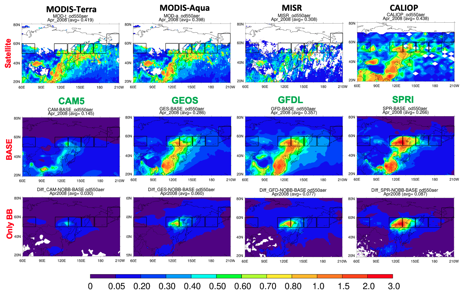
Figure 3 Spatial distribution of AOD at 550 nm in April 2008, from four satellite instruments (MODIS-Terra, MODIS-Aqua, MISR, and CALIOP) (Row 1); from four model BASE simulations (CAM5, SPRI, GEOS, and GFDL) (Row 2), and from biomass burning only AOD (BASE minus NOBB) (Row 3). Black boxes indicate the six focus regions.

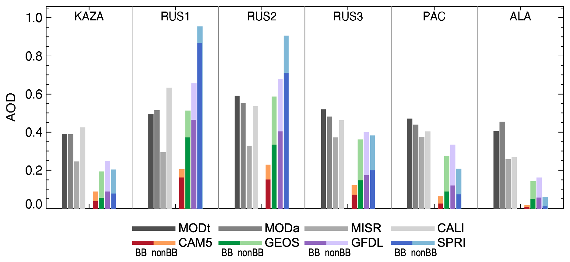
Figure 4 Regional mean AOD at 550 nm in April 2008 over the six focus regions (KAZA, RUS1, RUS2, RUS3, PAC, and ALA), derived from four satellite datasets where valid (MODIS-Terra, MODIS-Aqua, MISR, and CALIOP), and from four BASE model simulations (CAM5, SPRI, GEOS, and GFDL). Model AOD values are separated into contributions from biomass burning (BB; darker color) and non-biomass burning (nonBB, from NOBB runs; lighter color).

In Fig. 3 (first row), despite the limited availability of satellite aerosol retrievals at high latitudes, MODIS-Terra, MODIS-Aqua, MISR, and CALIOP all show high aerosol loading near Siberia-Lake Baikal (RUS1) and in the downwind regions (RUS2, RUS3, and PAC). Additionally, pronounced aerosol loadings are observed in East Asia and South Asia. Enhanced AOD in Kazakhstan (KAZA) is evident across all four satellite datasets. As shown in Fig. 4, the regionally averaged satellite AOD over KAZA ranges from 0.2 to 0.4, with MISR values about 40 % lower than MODIS. Over RUS1, regionally averaged AODs range from 0.3 to 0.6 across the four satellite products. Strong aerosol outflows from RUS1 toward RUS3 and PAC are also clearly visible in MODIS, MISR, and CALIOP data, with area-averaged AODs between 0.4 and 0.5. The area-averaged AOD from CALIOP is 0.3 over ALA (Alaska). Measurements from the ARCPAC and ARCTAS field campaigns (Warneke et al., 2009; Matsui et al., 2011) observed transported smoke aerosol and high trace gas concentrations in ALA during April 2008.

The second row of Fig. 3 displays the total AOD simulated by the models in their BASE runs (CAM5, SPRI, GEOS, and GFDL), all using the GFED4.1s biomass burning emission inventory and the model default smoke injection height settings. The corresponding BB AOD (BASE minus NOBB) is shown in Fig. 3 (third row). Over the BB source regions, all BASE runs (second row of Fig. 3) capture the high aerosol loading in RUS1, attributed to forest fires, and the slightly elevated AOD in KAZA due to agricultural fires (Warneke et al., 2009). However, the average model-simulated AODs differ significantly – by a factor of 2.8 over KAZA and 4.6 over RUS1, with CAM5 showing the lowest values (Fig. 4). The model-simulated AOD is lower than the MODIS AOD over KAZA, with varying degrees of agreement over RUS1: CAM5 largely underestimates, GEOS and GFDL align better with MODIS observations, and SPRI largely overestimates. Over RUS2, the models simulate slightly higher AODs than RUS1, consistent with MODIS observations. The higher AOD in RUS2 than RUS1 is attributed to the increase of the “background” (i.e., non-BB) AOD in RUS2 despite the decrease in BB AOD by all models (Fig. 4). In the RUS3 and PAC regions, all models underestimate AOD relative to MODIS observations, with an even larger underestimation in ALA.

In RUS1, BB dominates the total AOD in the BASE runs, contributing nearly 80 % (Fig. 4). Transported smoke from the RUS1 source region toward surrounding areas, for example, RUS2, RUS3, and PAC, is also significant in all models. However, the fraction of BB AOD is reduced as smoke plumes transport from the source to downwind regions; the longer the distance from the source, the smaller the BB AOD fraction becomes. More specifically, in RUS1, BB accounts for nearly 70 % to 92 % of the aerosol extinction across all models. In RUS3, the contribution of BB is reduced, as might be expected, ranging from nearly 58 % (CAM5) to 41 % (GEOS), and is further reduced in PAC, ranging from 38 % (CAM5) to 32 % (GEOS).

3.2 Sensitivity of total-column AOD to BB emission injection height and source-strength

The spatial distribution and regional mean AOD differences between the model sensitivity experiments and BASE runs are shown in Figs. 5 and 6, respectively. These results demonstrate the impact of constraining the fire plume injection height based on MISR retrievals (BBIH) and increasing the source-strength (BBEM).

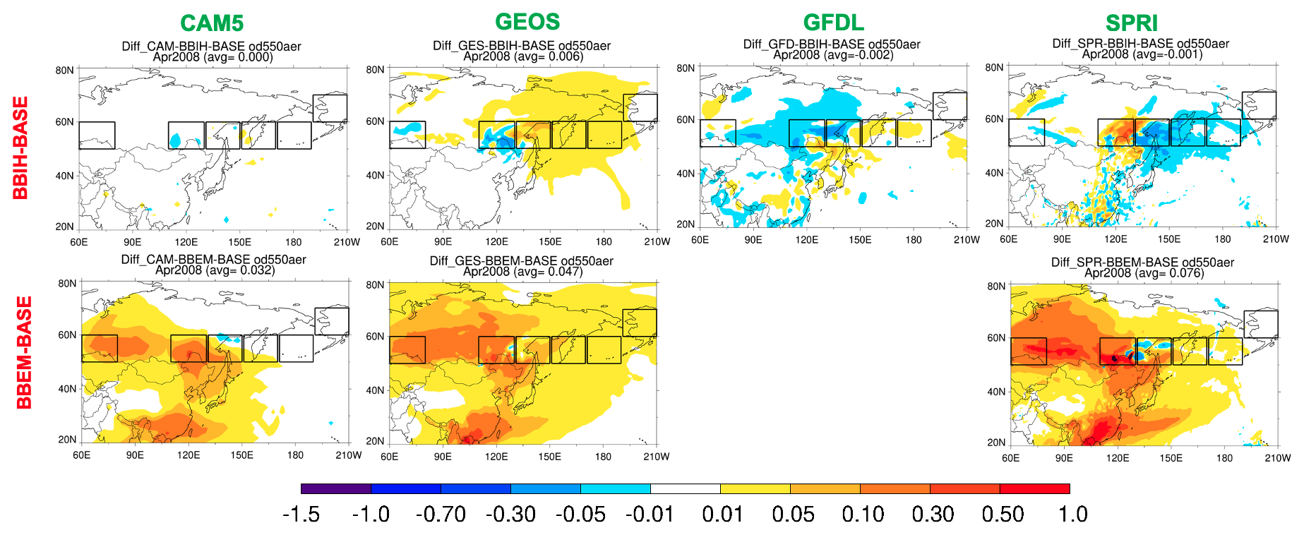
Figure 5 Spatial differences in AOD at 550 nm between BBIH and BASE (Row 1) and between BBEM and BASE (Row 2), simulated by the four models for April 2008. Only three models – CAM5, GEOS, and SPRI – submitted BBEM simulations. Focus regions are outlined in black.

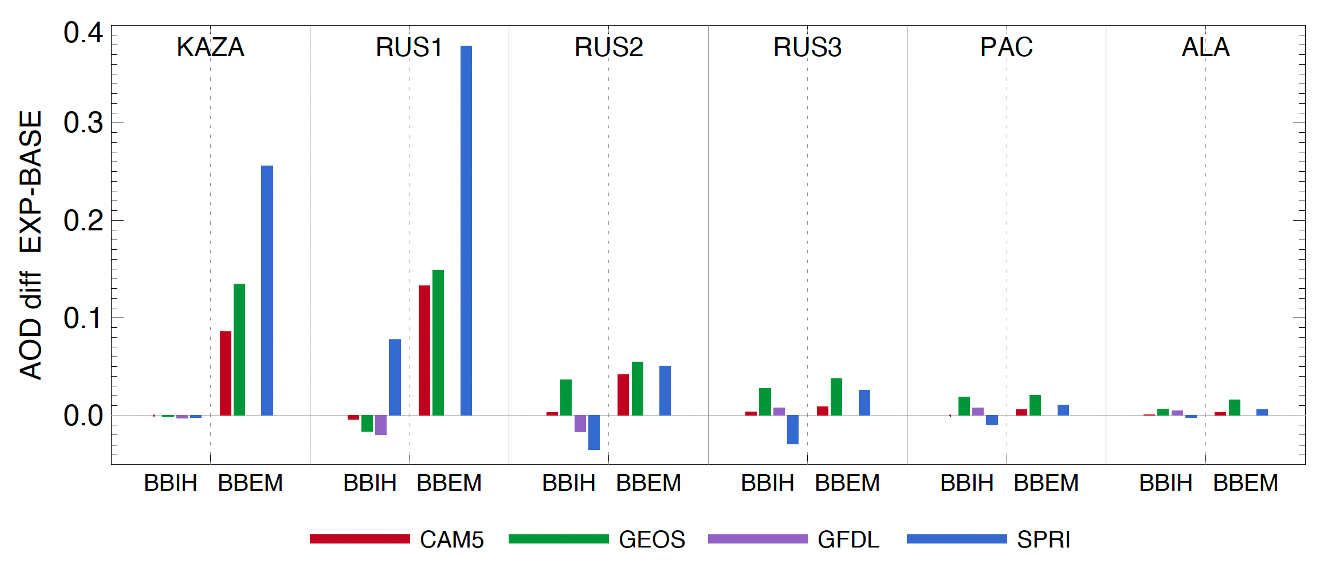
Figure 6 Regional mean differences in AOD at 550 nm for April 2008 across the six focus regions (KAZA, RUS1, RUS2, RUS3, PAC, and ALA), as simulated by four models (CAM5, SPRI, GEOS, and GFDL). Left in each panel: BBIH minus BASE; Right in each panel: BBEM minus BASE. Only three models, CAM5, GEOS, and SPRI, submitted BBEM simulations.

The AOD differences between BBIH and BASE (Fig. 5 top row and Fig. 6) remain relatively small – within ±0.05 for most models and less than 0.01 in CAM5. These results indicate that model responses to changes in biomass burning injection height vary. All models except SPRI show reduced AOD in RUS1 and increased AOD in the outflow regions (RUS2, RUS3, and PAC) in the BBIH run compared to BASE, consistent with the differences in vertical profiles among the models' default profiles and the MISR-based profile (Fig. 2b). For example, GEOS exhibits the expected pattern: lower AOD in RUS1 and higher AOD downwind, consistent with 55 % of emissions being injected above the PBL (0.68 km), facilitating greater long-range transport. CAM5 and GFDL emit 10 % less biomass burning smoke below 2 km in the BBIH run (90 %) compared to the BASE run (100 %). By contrast, SPRI shows the opposite behavior, with higher AOD in RUS1 and lower AOD downwind in BBIH relative to BASE. This pattern aligns with the SPRI vertical profile in BBIH, where nearly 90 % of the BB emissions were confined within the first 2 km, compared to 70 % in BASE (Fig. 2b), thereby limiting transport in BBIH.

Figure 5 (bottom row) shows the spatial distribution of AOD differences between the BASE and BBEM runs, with the corresponding regional mean differences summarized in Fig. 6. Only three models-CAM5, GEOS, and SPRI-submitted BBEM simulations, which used FEER1.0 BB emissions, whereas BASE runs used GFED4.1s. As shown in Fig. 1, GFED4.1s reports significantly lower BB emissions than FEER1.0, which is only 27 % of the FEER1.0 value in KAZA and 80 % in RUS1. Consistent with the higher emissions, BBEM simulations produce significantly larger AODs than BASE, especially near the source (e.g., AOD increased by 0.09 to 0.26 over KAZA and 0.13 to 0.38 over RUS1). However, the increase diminishes quickly in downwind regions (e.g., only 0.006 to 0.03 over PAC).

The discrepancies among satellite observations and models from source to downwind regions are further illustrated in Fig. 7. Figure 7a presents the satellite and model BASE simulations of regional mean AOD for RUS1, RUS2, RUS3, and PAC normalized to the source region RUS1. Figure 7b shows the model median AOD values from the BASE, BBIH, and BBEM experiments along with the satellite median values. Additionally, Table 4 summarizes these median values in all region and the percentages of model median to satellite median.

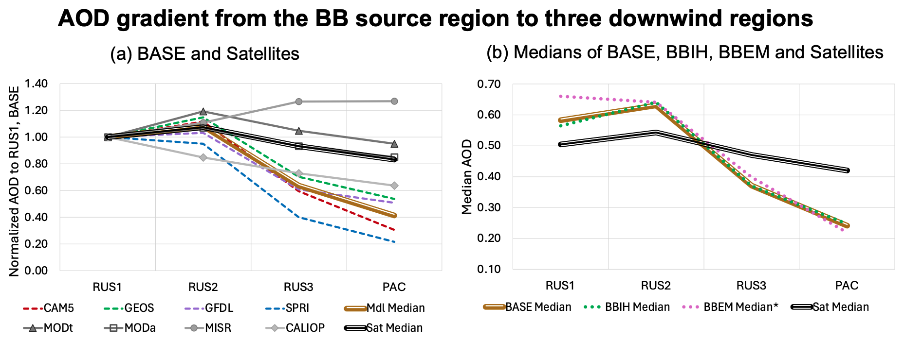
Figure 7 (a) The normalized 550 nm AOD gradient (relative to RUS1) from the BB source region RU1 to three downwind regions, based on satellite observations and the BASE simulations. (b) Comparison of the model median AOD values for four regions from the BASE, BBIH, and BBEM experiments, along with the satellite median values.

In Fig. 7a, BASE simulations from the individual models (dashed colored lines) as well as the model median (thick brown line) exhibit steeper AOD declines from RUS1 toward PAC compared to all the satellite products (solid grey lines) and the multi-satellite median (thick black line). Among the models, the source-to-downwind decrease of AOD is steepest in SPRI (blue dashed line), with a 78 % reduction from RUS1 to PAC, compared to GEOS (green dashed line), with 46 % reduction. Meanwhile, the differences among the satellite products in source-to-downwind gradient reflect the differences in sampling and data averaging approaches (see Sect. 2.3). Overall, although the BASE model median is 15 % higher than the satellite median over RUS1, it captures only 57 % of it over PAC (Table 4). This pattern suggests that the models may underestimate long-range aerosol transport or overestimate aerosol removal processes during transport. We discuss this further in Sect. 4.

To assess how model behavior of source-to-downwind gradient changes with the BBIH and BBEM experiments, Fig. 7b presents the model-median AOD values over RUS1, RUS2, RUS3, and PAC from the BASE, BBIH, and BBEM simulations, along with the satellite medians for comparison. The results clearly show that constraining biomass burning injection heights using monthly MISR plume data (BBIH) or increasing emission strength (BBEM) leads to only modest changes near the source region (RUS1) and does not significantly improve aerosol persistence during downwind transport. Quantitatively, the BBIH experiment produces an AOD that is 3 % lower than BASE in RUS1 and 2 % higher in PAC, directionally consistent with expectation, but much too small (or even negligible) to significantly reduce the discrepancy. The limited impact likely arises from differences in default injection heights among models: GFDL and CAM5 already use injection heights similar to MISR, whereas SPRI injects higher and GEOS injects lower than MISR. Consequently, the overall change in the multi-model median is minimal. Meanwhile, the median model AOD in the BBEM experiment (but lacking the GFDL model) exacerbated the high AOD bias by almost 20 % in RUS1 from the bias in the BASE simulation, but the enhancement diminishes rapidly along the transport pathway, resulting in only a few percentage difference from BASE downwind. Notably, the higher BB emission from FEER1.0 does help increase the AOD in KAZA, another source region, making it much closer to the satellite data (Table 4).

Table 4 The medians of regional mean AOD from satellites and model simulations.

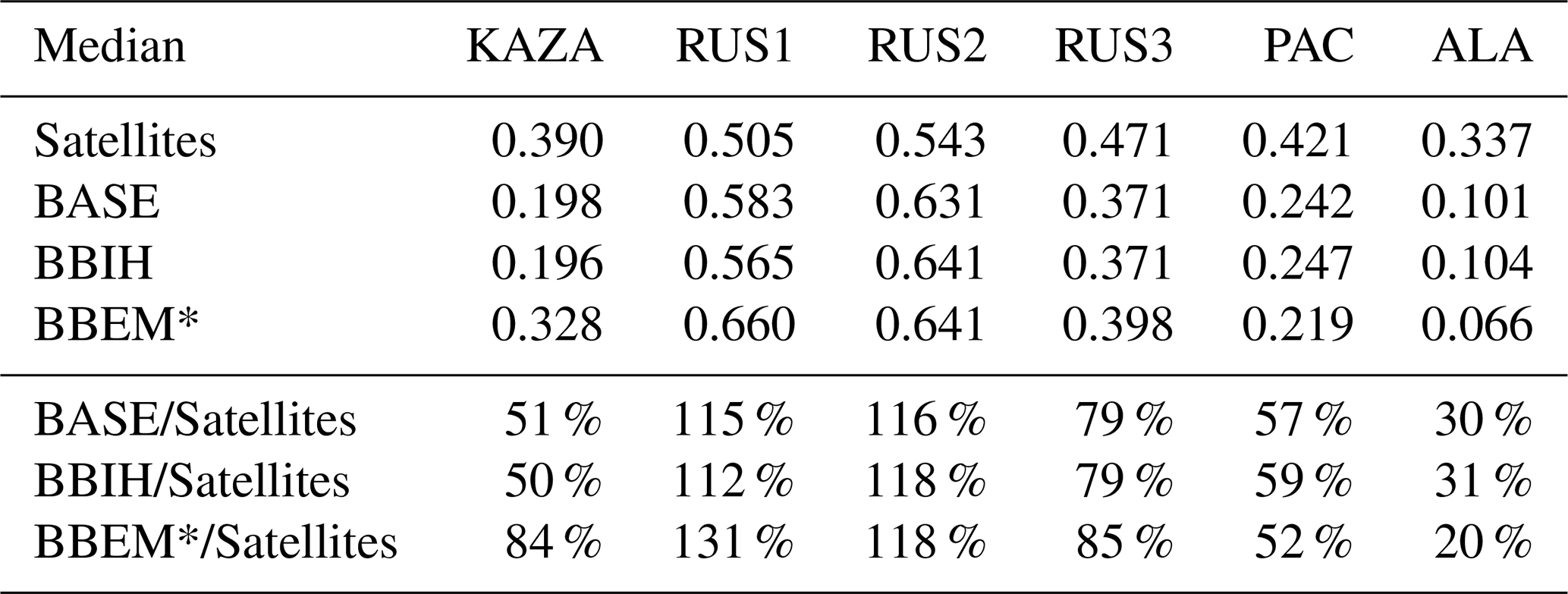
* GFDL did not provide results for this experiment.

As AOD represents only the integrated vertical column aerosol loading, Sect. 3.3 and 3.4 further examine the effects of biomass burning injection height and emission amount on surface aerosol concentration and vertical profiles, respectively.

3.3 Sensitivity of surface mass concentration to BB emission injection height and source-strength

The surface mass concentrations of BB OA (BASE minus NOBB) across all four models are shown in the first row of Fig. 8. We find that biomass burning emissions contribute to surface OA mass concentrations by up to 50 µg m⁻³ in KAZA and more than 100 µg m⁻³ in RUS1, especially in the GEOS model. The difference in surface OA mass concentration between the BBIH and BASE is shown in the second row in Fig. 8. Both CAM5 and GEOS simulate reduced surface mass concentrations in BBIH over the source regions of KAZA and RUS1, up to ∼50 µg m⁻³, but the changes are small toward the downwind regions. By contrast, SPRI shows the opposite response, as BBIH for this model leads to increased surface aerosol mass near the source region. This behavior is consistent results shown in Sect. 3.2, where we found that SPRI also produced more AOD near the source region in the BBIH run due to the higher default BB injection height in the BASE simulation than the MISR injection height in the BBIH simulation. Interestingly, CAM5 and GFDL use the same default BB injection scheme in BASE, but CAM5 shows lower OA concentrations in BBIH than BASE in both the KAZA and RUS1 BB source regions, but GFDL shows higher OA concentrations in KAZA and lower concentrations in RUS1.

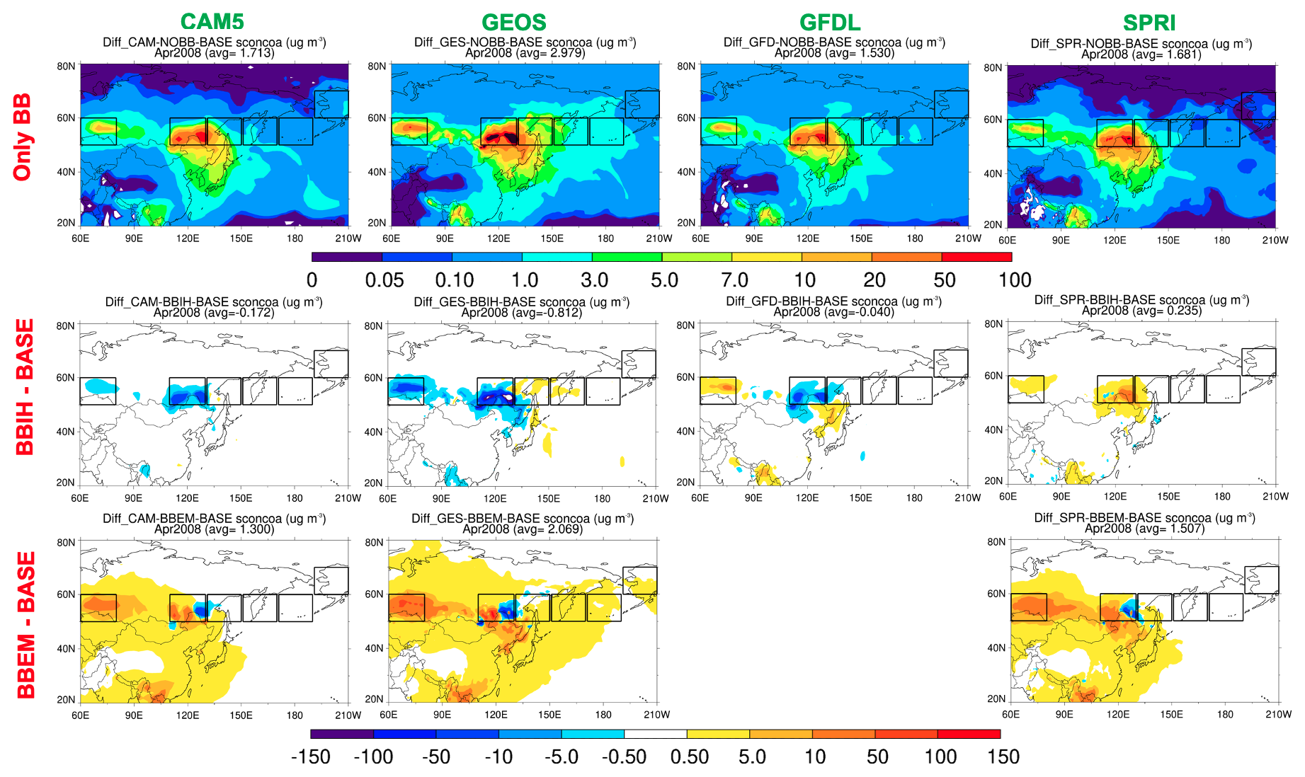
Figure 8 Spatial distribution of differences in surface OA concentrations for April 2008 across four models: CAM5, SPRI, GEOS, and GFDL. Row 1: Only BB (BASE minus NOBB). Row 2: BBIH minus BASE. Row 3: BBEM minus BASE. Note that only CAM5, GEOS, and SPRI provided BBEM simulations.

The third row in Fig. 8 presents the difference between BBEM and BASE. As expected, higher emission leads to higher surface concentration; all three models show widespread surface OA concentration increases in the BBEM run compared to BASE, both near the source and the outflow regions. The reduction of OA in the eastern part and the southwestern corner of RUS1 is due to the shift in BB emission locations between GFED4.1s and FEER1.0.

3.4 Sensitivity of vertical aerosol extinction profile to BB emission injection height and source-strength

Figure 9 presents the CALIOP aerosol extinction vertical profiles in April 2008 along with the aerosol extinction vertical profiles from the four participating models in six regions (KAZA, RUS1, RUS2, RUS3, PAC and ALA). Relevant statistics are listed within each panel.

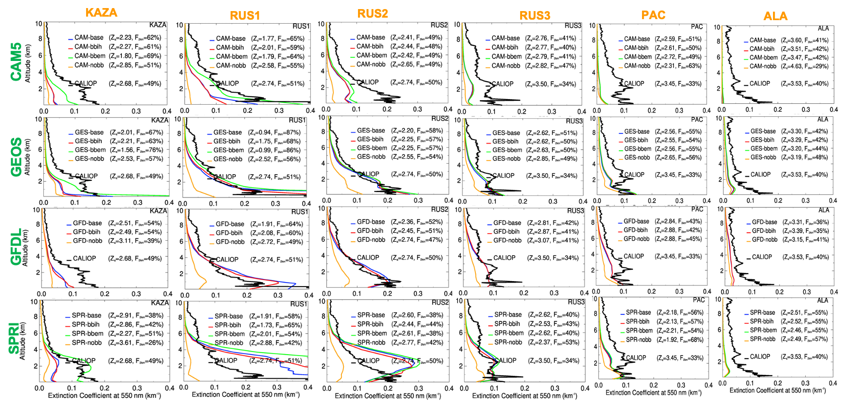
Figure 9 Vertical profiles of aerosol extinction in source and downwind regions. Aerosol extinction profiles for April 2008 from four models (CAM5, GEOS, GFDL, and SPRI), averaged over six regions. Column 1-2: KAZA and RUS1 (source regions); Columns 3–6: RUS2, RUS3, PAC, and ALA (downwind regions). Each panel includes CALIOP observations (thick black curves) and model outputs from four experiments – BASE, BBIH, BBEM, and NOBB – shown as colored curves. Summary statistics are listed beside the legend: Z_a (mean aerosol layer height) and F_2 km (fraction of AOD within the lowest 2 km).

To evaluate the vertical profiles, we used two vertical profile metrics, the average aerosol layer height, Z_a, and the fraction of total-column AOD in the lowest 2 km, F_2 km. Following Koffi et al. (2012), Z_a is calculated as:

$$\begin{array}{}\text{(1)}& Z_{\mathrm{a}}={\displaystyle \frac{\sum _{i=\mathrm{1}}^k(b_{\mathrm{ext},i}\cdot Z_i)}{\sum _{i=\mathrm{1}}^k{b}_{\mathrm{ext},i}}}\end{array}$$

Here k is the total number of layers in each column, b_ext,i is the aerosol extinction for layer i within the column, and Z_i is the layer thickness for layer i. F_2 km is obtained by integrating the aerosol extinction from the surface to 2 m and dividing by the CALIOP AOD, obtained by integrating the reported aerosol extinction throughout the atmospheric column. Note that because the upper-bound CALIOP data are used, which exclude data below the CALIOP detection limit in producing the level 3 mean aerosol extinction (Sect. 2.4), the absolute values of CALIOP aerosol extinction shown in Fig. 9 could be biased high, especially at higher altitudes, where CALIOP tends to encounter the detection limit more often than in the PBL. As such, the calculated CLAIOP Z_a could be skewed toward higher altitudes, thus reducing the F_2 km.

The comparisons in Fig. 9 show that over the source region KAZA (1st column), the aerosol extinction profiles from the model BASE simulations (blue lines) are ∼40 %–80 % lower than the “upper-bound” CALIOP throughout all altitudes, with non-BB aerosol exceeding BB aerosol extinction, consistent with the BASE simulations of AOD (Fig. 4). This suggests that the GFED4.1s emissions used in the BASE runs is likely too low over KAZA. By contrast, over the source region RUS1 (2nd column), aerosol extinction below 2 km altitude from the BASE simulation is higher than the “upper-bound” CALIOP data (see Sect. 2.3) for GEOS, GFDL, and especially SPRI, but is lower than CALIOP for CAM5. The simulations also show that BB aerosol is the main contributor to total aerosol extinction in RUS1. The wide range of model-simulated aerosol extinction in the lower atmosphere can be partly attributed to differences in mass extinction efficiency (MEE) that converts aerosol mass to aerosol extinction (discussed in Sect. 4.1 below) and partly to the OA $/$ OC ratio used in models (see Table 3). Both parameters are highest in SPRI and lowest in CAM5. Above 5 km, all model-simulated aerosol extinction values are lower than CALIOP. Consistent with the AOD comparisons (Sect. 3.1), the model-simulated aerosol extinction decreases in downwind/remote regions (RUS2 to ALA, 3rd to 6th columns) much faster than the CALIOP data.

Figure 9 also indicates that the differences produced in the BBIH (red lines) and BBEM (green lines) simulations are seen primarily over the source regions (KAZA and RUS1), especially below 3 km, in the direction consistent with the differences between BBIH and BASE for injection height or between BBEM and BASE for emission amount. For example, the GEOS overestimation of aerosol extinction below 2 km from the BASE runs is reduced in the BBIH runs, because the default BB emission in BASE is confined entirely within the PBL but MISR-based injection height in BBIH releases 55 % of emission above the PBL (Fig. 2). This leads to improved agreement with the CALIOP data in the source region. On the other hand, the BBIH run makes the overestimation by SPRI in RUS1 even more than in the BASE run, because the MISR-based injection places a greater fraction of smoke below 2 km than the default SPRI BB injection height (Fig. 2). Meanwhile, higher BB emission in BBEM significantly improves the agreement of aerosol extinction profiles between model and CALIOP in KAZA, especially below 3 km. In all cases, the differences among BASE, BBIH, and BBEM simulations become much smaller, even negligible in downwind regions.

We further use the parameters Z_a and F_2 km to compare the aerosol vertical placement between models and CALIOP. As shown in Fig. 9, the Z_a from CALIOP is 2.7 km over the source regions KAZA and RUS1 as well as in the immediate downwind region RUS2, with about half of the AOD situated below 2 km (F_2 km=50 %–51 %). The Z_a increases to 3.5 km further downwind over RUS3 and PAC, where about $\mathrm{1}/\mathrm{3}$ of AOD is located below 2 km (F_2 km=33 %–34 %). In the more distant ALA region, where the BB influence is expected to be reduced, the Z_a is maintained at 3.5 km, with 40 % of AOD below 2 km.

In comparison, the model-calculated Z_a values from the BASE runs are lower than CALIOP and the F_2 km values are higher than CALIOP in all regions, except SPRI in KAZA, which goes in the opposite direction. Over the source region RUS1, the Z_a is lower by less than 1 km in CAM5, GFDL, and SPRI but by 1.8 km in GEOS. Correspondingly, the F_2 km values from all models is higher than CALIOP, from 7 %–14 % in CAM5, GFDL, and SPRI to 36 % in GEOS. These values are consistent with the differences in the default BB injection heights among models. The differences between all models and CALIOP in the downwind regions converge to less than 1 km for Z_a and to less than 17 % for F_2 km. These values in the BBEM runs are very similar to those in the BASE runs in all regions except KAZA, as expected, as both experiments use the same BB injection heights, and the small differences between these two experiments can be attributed to the changes of BB contributions to total aerosol extinction. On the other hand, the Z_a values in the BBEM runs are 0.4–0.7 km lower and F_2 km are 7 %-13 % higher than those in the corresponding BASE runs, because the higher BB emissions in BBEM significantly increase the BB aerosol fractions near the surface. That is, this tends to produce lower Z_a and higher F_2 km than non-BB aerosols (Fig. 9), making discernable differences in Z_a and F_2 km in the total aerosol extinction.

The BBIH simulations make the most noticeable differences in Z_a and F_2 km in the source regions. In RUS1, for example, Z_a increases by ∼0.2 km from the BASE in CAM5 and GFDL to be a little closer to the CALIOP Z_a value; meanwhile Z_a decreases by 0.2 km in SPRI from the BASE run, creating a greater departure from CALIOP. Correspondingly, F_2 km decreases by a few percent in CAM5 and GFDL but increases in SPRI. The largest magnitude changes in RUS1 are seen in the GEOS model: Z_a from the BBIH run increases by 0.8 km and F_2 km decreases by ∼20 % compared to the BASE run. Similar trends are also seen in KAZA, although the magnitudes are much smaller. Again, all these changes in BBIH from BASE are attributable to the difference in BB injection height in these two experiments. However, as we have shown in the comparison of AOD and extinction profiles, the differences between BASE and BBIH quickly become trivial in downwind regions.

However, there are uncertainties and bias in the data as well. The upper-bound CALIOP data likely have a larger positive bias at higher altitudes (see discussion Sect. 4.2), leading to Z_a values about 1 km higher than the lower-bound CALIOP data (Kim et al., 2019). Therefore, it is difficult to draw definitive conclusions about the vertical displacement of model-simulated extinction based on the CALIOP data showing here.

4 Discussion

4.1 Sources of aerosol discrepancies among models

A key contribution of the current study is the ability to intercompare model performance in simulating smoke-transport. To this end, we investigated the sources of discrepancies among models by examining the model-simulated OA, the major BB aerosol component, averaged over four source-to-downwind areas, RUS1, RUS2, RUS3, and PAC, for April 2008. This analysis includes five key variables from the BASE runs by the four models: (1) total emission from biomass burning and anthropogenic sources, (2) loss frequency due to wet and dry deposition, (3) column mass load, (4) MEE, and (5) AOD. Here, the loss frequency is calculated as the ratio of column mass load to total (wet + dry) deposition rate, and MEE is the ratio of AOD to column mass load. Results are summarized in Table 5 for the individual models, along with the multi-model median, inter-quartile range (IQR) normalized by the median (expressed as a percentage to indicate inter-model spread), and the ratio of maximum to minimum values among the models. Figure 10 further illustrates the model diversity, expressed as the percentage deviation of each model from the multi-model median for each variable. For clarity, the deposition residence time in Fig. 10 is calculated as the reciprocal of the loss frequency, to highlight whether shorter residence time leads to lower mass load, as expected).

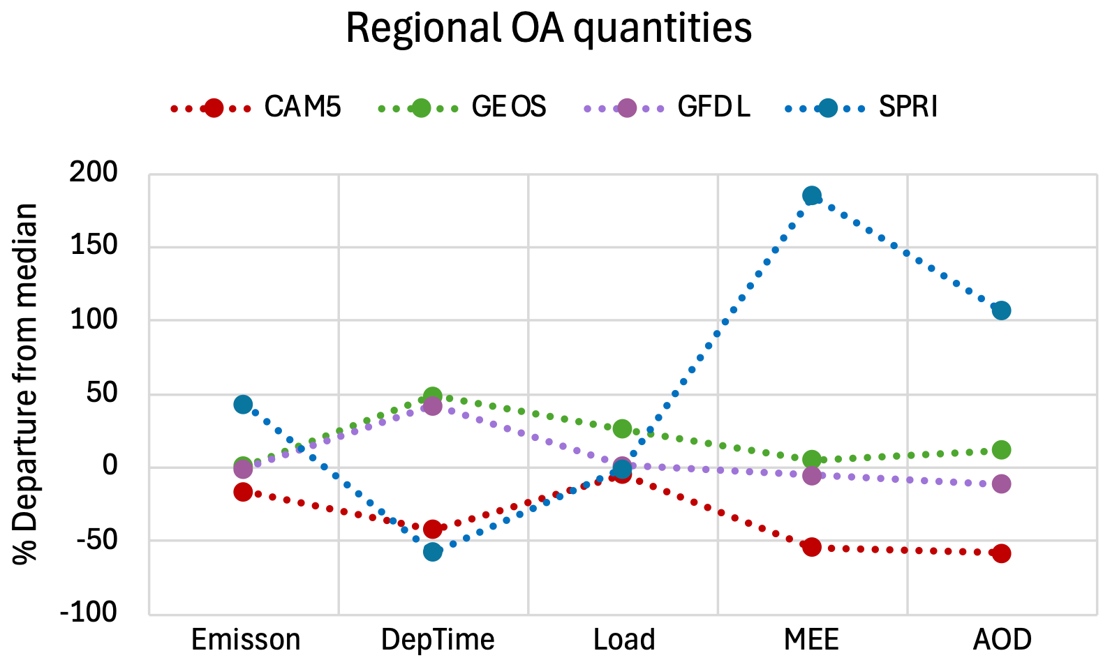
Figure 10 Comparison of key model-simulated variables determining OA AOD in each model for April 2008, averaged over four regions from RUS1 to PAC. Colored symbols represent the percentage deviation of each model from the multi-model median. The actual values from individual models, along with the multi-model statistics (median, IQR $/$ median, and max $/$ min), are listed in Table 5.

Table 5 Total emission, area-mean deposition loss frequency, column mass load, MEE, and AOD for OA averaged over RUS1, RUS2, RUS3, and PAC for April 2008 from model BASE simulation, along with associated statistical values.

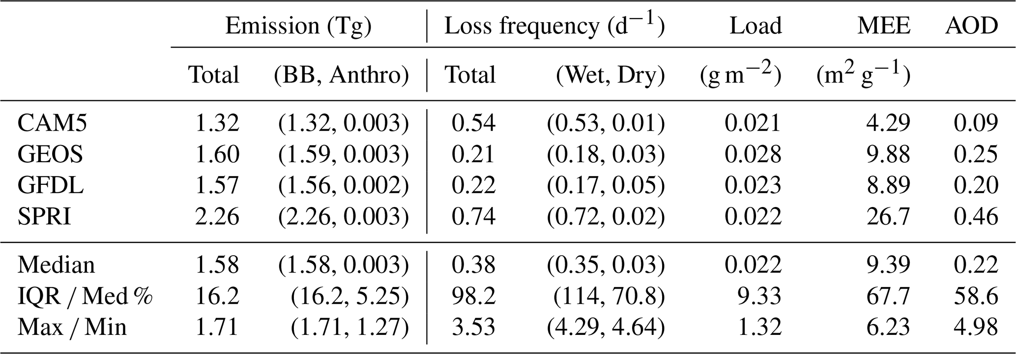
Fundamentally, sources and removal rates determine the mass load, and the mass load and MEE together determine the AOD. In this study region and period, BB emission is the predominant source of OA, accounting for more than 99 % of the total OA emission. For the OA loss due to deposition, all models agree that wet deposition is the major removal process, with the loss frequency 3 to 50 times higher than that of dry deposition (Table 5). Interestingly, despite significant differences in OA emissions and deposition rates among the models, the disparity of the resulting OA loads is surprisingly small. The inter-model spread in OA mass load, indicated by the IQR divided by the median, is only 9.3 %, compared to 16 % for emissions and 98 % for loss frequency. This small spread in OA mass load is mainly due to the compensating effects of emission and removal frequency. For example, SPRI has the highest OA emission (because of its assumed highest OA $/$ OC ratio among models at 2.6; Table 3) but also the fastest removal rate (i.e. the shortest deposition residence time), whereas GFDL has much lower emission but a significantly slower removal rate (i.e., longer deposition residence time). As a result, they end up with very similar OA mass load despite contrasting parameter choices. Note that this analysis does not account for OA inflow and outflow due to transport, nor for any secondary OA formation from volatile organic compound oxidation in the regional source/sink budget. Therefore, mass is not strictly conserved within the study region. Nevertheless, we are considering by far the dominant controls on OA in this case, so the key findings regarding the inter-model diversity remain robust.

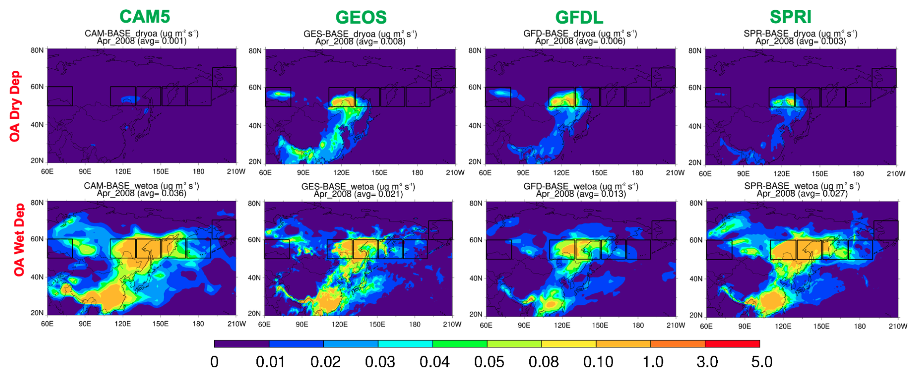
Figure 11 Spatial distribution of OA dry deposition (units: $\mathrm{\mu }\mathrm{g}{\mathrm{m}}^{-\mathrm{2}}{\mathrm{s}}^{-\mathrm{1}}$) and wet deposition for April 2008, as simulated by four models (CAM5, GEOS, GFDL, and SPRI) in their BASE runs.

Although OA mass loads are relatively consistent across models (max $/$ min = 1.3 and IQR $/$ median = 9.3 %), the differences in OA AOD are very large (max $/$ min = 5 and IQR $/$ Median = 59 %). This large spread in AOD is primarily attributable to substantial differences in MEE (max $/$ min = 6.2 and IQR $/$ median = 68 %). For instance, SPRI exhibits an extremely high MEE at 26.7 m² g⁻¹, whereas CAM5 has the lowest value of 4.3 m² g⁻¹ (Fig. 10 and Table 5). This large contrast in MEE results in the large difference in OA AOD. Theoretically, MEE depends on aerosol optical and microphysical properties, including particle refractive indices, size distribution, dry density, and hygroscopic growth under ambient humidity (e.g., Hess et al., 1998; Chin et al., 2002). The results in Fig. 10 indicate that SPRI assumes remarkably strong hygroscopic growth for OA particles, making MEE about three times the multi-model median value, whereas CAM5 assume much lower water vapor uptake ability, producing a MEE value roughly half the multi-model median. The global spatial distribution of OA mass load, OA AOD, and OA MEE are shown in Fig. A2.

Clearly, using the remotely sensed AOD as a constraint is necessary to produce realistic model simulations, but by itself, it is insufficient for evaluating the underlying factors that contribute to model AOD diversity. To improve future aerosol modeling and AeroCom intercomparisons, this study – along with Petrenko et al. (2025) – strongly recommend constraining MEE values (ranging from 4.3 to 26.7 in this study) and OA $/$ OC ratios (ranging from 1.4 to 2.6 in this study). Unfortunately, there are no statistically robust observational constraints for MEE, emission, deposition, and mass load covering the major aerosol types, key variables that each play a critical role in determining AOD (e.g., Kahn et al., 2023). Further, the OA $/$ OC ratio does exhibit a wide range in nature that depends on many factors, including the burned vegetation type, chemical structure of OA compounds, formation of OA from different precursors, aging of the airmass, and meteorological conditions in the environment. Although the range of OA $/$ OC ratio in this study is within the observed values (e.g., Malm et al., 1994; Aiken et al., 2008; Hodzic et al., 2020), more systematic measurements of this ratio are highly desirable to obtain robust statistics for the most probable values under various conditions.

4.2 Discrepancies between model and satellite observations

As presented in Sect. 3, the models show a stronger meridional decline in AOD from the source regions to the downwind regions, compared to satellite data (e.g., Figs. 4, 7, and Table 4). The models also significantly underestimate the aerosol extinction in the middle to upper troposphere compared to CALIOP lidar data (Fig. 9). These discrepancies persist across all experiments and models. Possible explanations include (a) excessively rapid aerosol wet removal along the transport pathways, (b) underestimated BB injection height (with both model default assumptions and monthly MISR values lower than actual plume height in our study area), and (c) insufficient vertical mixing in the models. Below, we evaluate each explanation in turn.

Excessive wet removal. Our model budget analysis indicates that wet deposition is the dominant removal process for OA across all models (Table 5). This is expected, given the submicron size and hygroscopic nature of OA smoke particles. Among the models, Fig. 11 and Table 5 show that CAM5 and SPRI exhibit significantly higher wet depositional loss rates than GEOS and GFDL, and their average deposition residence times over the four regions from RUS1 to PAC are ∼50 % lower than the multi-model median, whereas the GEOS and GFDL values are 50 % higher. This behavior is consistent with the steeper meridional reduction of AOD from RUS1 to PAC in CAM5 and SPRI than in the other two models (Fig. 7a). The inter-model differences likely stem from differences in model representations of precipitation amount and wet scavenging parameterization, among other factors. A recent paper by Zhong et al. (2022) analyzing biomass burning aerosol lifetimes in the AeroCom global models found that the BB aerosol lifetime is strongly correlated with precipitation, indicating that wet deposition is a key driver for BB aerosol burden. Notably, however, even with much smaller loss frequency in the GEOS and GFDL models, their AOD decrease from RUS1 to PAC remains far more rapid than indicated by the satellite-retrieved AOD.

Although the dominance of wet deposition is not surprising, the degree to which it varies among models-and its potential role in the underestimation of downwind AOD and vertical aerosol extent warrants further investigation. Future AeroCom experiments might consider performing additional sensitivity studies that involve changing the removal rates and/or implementing standardized diagnostics and tracer experiments to better quantify and compare aerosol removal pathways across models. In addition, improved wet removal metrics should be considered. Recent work (Hilario et al., 2024) suggests that precipitation intensity and relative humidity are more robust indicators of wet-scavenging efficiency, implying that models may benefit from incorporating these meteorological controls into wet-deposition parameterizations.

Underestimated BB injection height. As shown in Sect. 3 (Figs. 5 and 6), the change of model simulated AOD in BBIH from BASE depends on BB injection profile differences between the default used in BASE and the MISR scheme in BBIH. Figure 2b shows that the GEOS default injection height (PBL scheme) is much lower than MISR, SPRI (fixed altitude scheme) is much higher than MISR, whereas GFDL and SPRI (Dentener scheme) are similar to MISR. As a result, GEOS gains the most notable improvement in BBIH. For example, in RUS1, the fraction of AOD below 2 km (F_2 km) improved significantly in BBIH, decreasing from 87 % in BASE to 68 % in BBIH, closer to the CALIOP-observed value of 51 %. This improvement reflects a shift from all BB emissions being confined within the PBL in the BASE run to 55 % of BB emissions being injected above the PBL in BBIH. In comparison, the default biomass burning injection heights in CAM5 and GFDL are relatively close to those retrieved by MISR, such that the differences between the BASE and BBIH simulations are minimal for these two models. In SPRI, however, which used a fixed altitude scheme in BASE that distributed emissions uniformly up to 3 km, the BBIH scheme degrades agreement with observed AOD distribution. This is because its default BB injection height is higher than MISR; using the MISR injection height puts more emission in the PBL (45 %–55 %) than the default (22-25 %), while increasing the fraction below 1 km from 30 % to 70 %. Although the changes in BBIH are still too small to substantially improve the agreement between models and satellites, these results demonstrate that the model simulations do respond to changes in injection height, and shifting the injection profile to place more smoke above 3 km would help.

We did not conduct a simulation combining both MISR-based injection heights and the FEERv1.0-G1.2 emissions (i.e., a BBIH + BBEM experiment), as our main goal in the current study is to disentangle the individual impact of a combined biomass burning injection height and emission strength. The impact of combined BBIH + BBEM experiment could be estimated from the BASE, BBIH, and BBEM experiments, with the assumption that the effects of injection height and emission strength are approximately multiplicative and independent, such that BBAOD${}_{\mathrm{BBIH}+\mathrm{BBEM}}={\text{BBAOD}}_{\mathrm{BBEM}}$ ($\mathrm{1}+{\text{BBAOD}}_{\mathrm{BBIH}}/{\text{BBAOD}}_{\mathrm{BASE}}$). However, given the small differences between the BASE and either the BBIH or BBEM results downwind and in the free troposphere, we do not expect that the BBIH + BBEM experiment would produce substantially better agreement between model and satellite data.

Regarding the injection height, the monthly and regional-mean MISR plume height is broadly representative of typical plume injection behavior (Val Martin et al., 2018; Junghenn Noyes and Kahn, 2025), but this approach might underrepresent extreme events or diurnal variability in plume rise, such as the strong April 2008 Siberian wildfires we focus on the current study. In addition, MISR observations (Val Martin et al., 2018), taken in the late morning (∼10:30 a.m. local time), tend to underestimate typical peak daytime plume heights, as only about 20 % of plumes rise above the boundary layer at that time, compared to ∼55 % by late afternoon (Ke et al., 2021). Future modeling should consider how injection profiles might be adjusted to address this limitation and better represent plume rise above 3 km. Providing observations to adequately constrain aerosol transport models in this respect might require applying the combination of near-source injection height from multi-angle imaging (e.g. MISR and follow-on multi-angle satellite imagers), and downwind aerosol-plume vertical distribution (e.g., CALIOP and subsequent space-based aerosol lidars) (Kahn et al., 2008).

Insufficient vertical mixing. Underestimation of aerosol extinction at higher altitudes by the models may also indicate insufficient convective or turbulent vertical mixing. It is difficult to attribute the difference between CALIOP and the models, as well as among different models, to the transport and/or removal processes without having adequate diagnostic tools. In that regard, implementing common tracers for transport and removal would be highly desirable to more precisely diagnose and attribute the causes responsible for these discrepancies. The models use different advection schemes, vertical diffusion parameterizations, and convective transport treatments, all of which can affect the vertical distribution of aerosols. However, a comprehensive evaluation of these processes is beyond the scope of the current study.

Lastly, our evaluation of the model-simulated aerosol fields in our case study mostly uses the remote sensing AOD and aerosol extinction profile optical products. As we show in previous sections, the MODIS and MISR AOD data have spatial gaps over high latitudes and in cloudy or partially cloudy situations, whereas the CALIOP data suffer from poor observability in low aerosol environments such as in the free troposphere, where the aerosol extinction is often below the CALIOP instrument detection limit. The differences between the mean CALIOP data with or without the assumed zero values under “clean” conditions can be 0.05 km⁻¹ in the lower troposphere and 0.02 km⁻¹ in the upper troposphere over the northwestern Pacific in spring (Kim et al., 2019), a range that could bound the range of model-simulated aerosol extinction vertical profile values, making quantitative assessment uncertain. Future model evaluation matrices should also involve aircraft data that provide more direct measurements of aerosol mass concentration, chemical composition, size distribution, optical properties, and vertical profiles, offering more reliable constraints on model processes. Understandably, the aircraft measurements are limited in space and time, and coordination with remove-sensing observations requires careful, strategic planning.

5 Conclusions

This BBEIH study addresses two key questions: (1) How sensitive are simulated near-source and downwind plume characteristics – including vertical aerosol distribution, near-surface concentration, and AOD – to the injection height of biomass burning emissions? and (2) To what degree does the choice of biomass burning emission inventory or source-strength affect smoke dispersion?

We evaluated the sensitivity of smoke aerosol dispersion to smoke injection height and source-strength in four global models for the year 2008 under the umbrella of the AeroCom Phase-III experiment, with a focus on the Siberian wildfires near the Lake Baikal region in eastern Russia during April. Each model performed four simulations: (1) BASE, all models used the GFEDv4.1s emission inventory and applied the model-specific BB injection height; (2) BBIH, same as BASE, but the vertical distribution of BB emissions was constrained by the statistically based monthly MISR plume injection heights in the study region; (3) BBEM, same as BASE, but with GFED4.1s replaced by the FRP-based biomass burning emission inventory FEER; (4) NOBB, BB emissions were excluded entirely. Unlike previous studies using a single model, this work compares BB emission injection height representations across multiple models. We assess each model's default vertical distribution approaches (e.g., Dentener scheme, PBL scheme, and fixed height scheme) and then apply MISR-constrained injection height uniformly to evaluate its impact.

In the BASE simulations, all models captured the AOD maximum associated with the Siberian wildfires near the Lake Baikal region. In the RUS1 source region, biomass burning dominates the total AOD, contributing nearly 80 %. However, AOD levels varied notably among models: CAM5 significantly underestimates AOD, SPRI substantially overestimates it, whereas GEOS and GFDL show better agreement with MODIS observations. Despite these differences, a common feature across all models is the much more rapid AOD decrease from RUS1 to PAC than the satellite retrievals. Specifically, all models consistently underestimate the strong aerosol outflow observed over the western North Pacific, where the satellite-derived median AOD is 0.42, but the model ensemble median in this region is only 0.24, representing a 43 % underestimation. This pattern suggests that all models either have insufficient long-range aerosol transport or overestimate aerosol removal processes during transport. Furthermore, compared to the upper-bound CALIOP data, all models overestimate the fraction of AOD below 2 km by 3 %–36 % in RUS1, 6 %–17 % in RUS3, 9 % to 24 % in PAC, and 1 %–15 % in ALA, but are more similar in RUS2. Notably, CALIOP detects aerosol layers extending above 6 km, from the source to downwind regions – these features are not reproduced by any of the simulations. The discrepancy indicates excessive smoke concentration near the surface across all models and partly explains the overly rapid AOD decrease during downwind transport. However, some of the discrepancies between CALIOP and models can also be attributed to the overestimation of aerosol extinction at high altitudes in the upper-bound CALIOP data.

In the BBIH run, all models applied a consistent, MISR-based monthly vertical distribution of fire injection: 45 % of the smoke was emitted within the planetary boundary layer in the source region (RUS1) and 55 % in KAZA, with the remainder above, following the MISR-derived weighting function. This led to a redistribution of AOD, surface OA mass concentration, and vertical profiles in most models; the degree of improvement depended on the difference between the model default injection height in BASE and the MISR injection height in BBIH. In general, the direction of AOD change was in the right direction to improve the model agreement with satellite AOD, but the magnitude of AOD change was much too small to make a significant impact on vertical smoke redistribution in the downwind regions or to reduce the persistent AOD underestimation there. This result suggests that a greater portion of BB emissions should be emitted to altitudes higher than those observed by the monthly MISR plume height used in BBIH runs in this case study, which is not entirely surprising given the intensity of the fires associated with the event considered in here. Furthermore, the MISR observations in the late morning (Terra satellite overpass time) would underestimate the typical peak plume heights in the afternoon. In comparison, the BBEM experiment, which employed higher BB emission in the two major source regions, KAZA and RUS1, by factors of 3.7 and 1.2 than the BASE experiment, resulted in significant increases in AOD near the source regions. Although this increase helped improve model-simulated AOD in the KAZA region, it led to more overestimation of AOD in RUS1 and RUS2. Moreover, the models were unable to sustain the increase in downwind regions, as would be needed to improve the agreement with satellites there, nor did it increase the aerosol extinction at higher altitudes near-source or downwind.

Overall, our results indicate that increasing biomass burning emission strength and simple modifications to the injection height alone are insufficient to reproduce observed aerosol distributions. This study suggests several possible issues: (a) aerosols may be removed too quickly during transport, (b) the BB injection height profile derived from monthly MISR over the boreal region may still be biased toward the lower atmosphere, at least in this case study, and (c) vertical mixing is insufficient in the models.

We also investigated the sources of discrepancies among models. As discussed in Sect. 4, we found that different choices of MEE and OA $/$ OC ratio, along with differences in aerosol loss rate, play a major role in creating diversity among modeled AOD and in the discrepancies between model and satellite AOD. Similar findings are reported in Petrenko et al. (2025), which used 10 models, including the CAM5, GEOS, and SPRI models applied in the current study as well. Equally critical is quantitatively assessing transport efficiencies in both the vertical and horizontal dimensions, and of aerosol removal, which would require implementation of common diagnostic tracers in the models. These considerations are important for better understanding model-simulated smoke near-source as well as downwind and determining how to make model improvements. The proposed diagnostics should help in designing the upcoming AeroCom Phase IV experiments. Further, there is a lack of critical measurements for constraining particle microphysical properties such as MEE, and aerosol properties and processes such as OA $/$ OC ratio, loss rates, and aerosol vertical distributions. These would be required to make the implied model adjustments consistently and appropriately (e.g., Kahn et al., 2023). Although the present study is unable to address these issues, it highlights the directions in which further advances are needed.

Some of our results align with those of previous studies, which lends confidence to our conclusions and suggests greater applicability than just for the cases included here. We suggest that future experiments (e.g., AeroCom Phase IV) expand the analysis to include different fire regimes. We emphasize that this is the first coordinated multi-model intercomparison that systematically isolates the effects of injection height and emission strength using a harmonized experimental design and satellite-based constraints. The novelty of this work lies in the cross-model comparisons, the quantification of inter-model variability, particularly in vertical aerosol distribution and long-range transport, and the identification of relative differences in underlying model attributes.

Appendix A

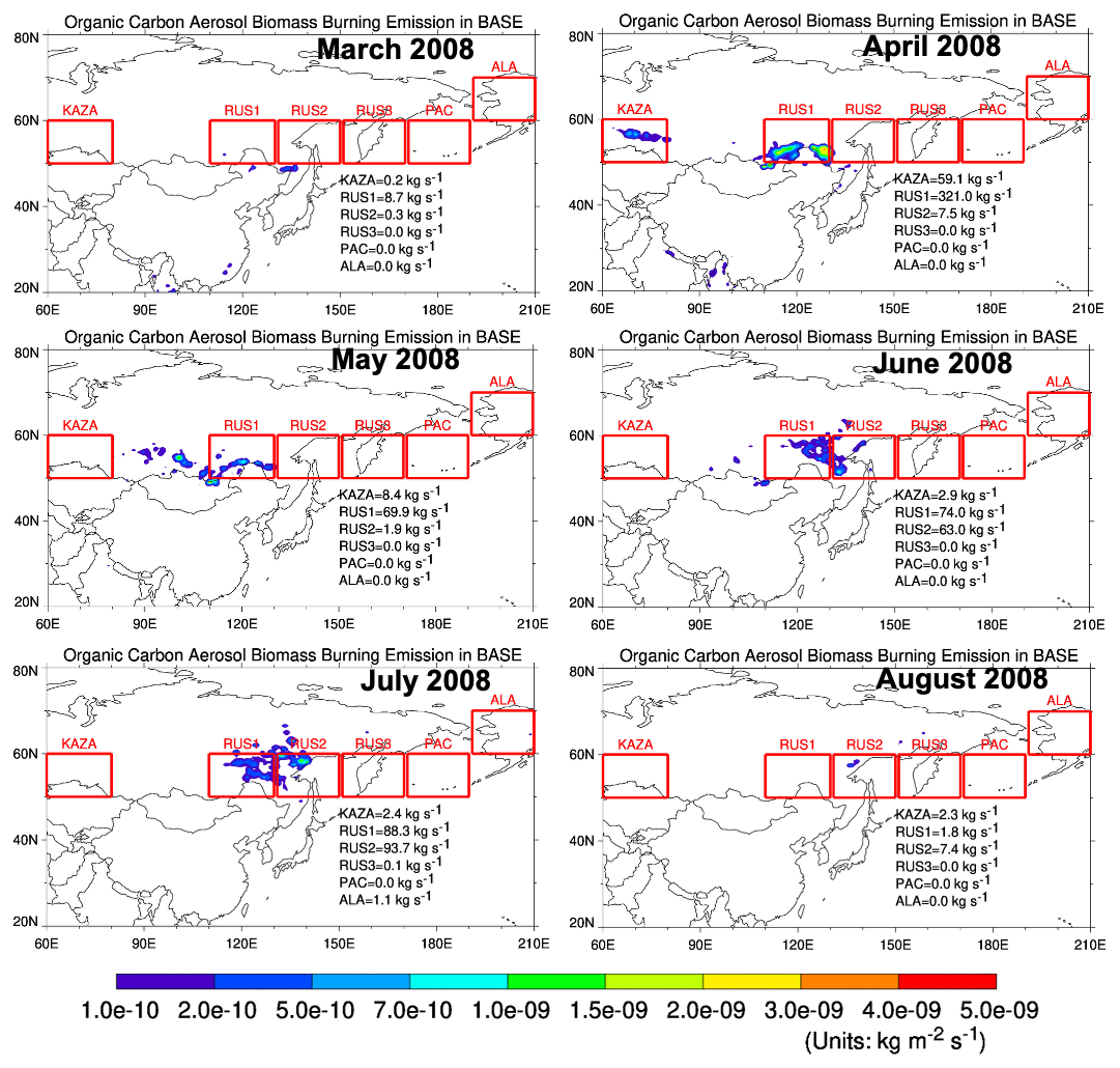
Figure A1 Spatial distribution of monthly mean organic carbon aerosol emissions from biomass burning from March to August 2008, based on the GFED4.1s inventory (from the BASE run), in units of $\mathrm{kg}{\mathrm{m}}^{-\mathrm{2}}{\mathrm{s}}^{-\mathrm{1}}$. The six focus regions are highlighted, with total emissions indicated for each region.

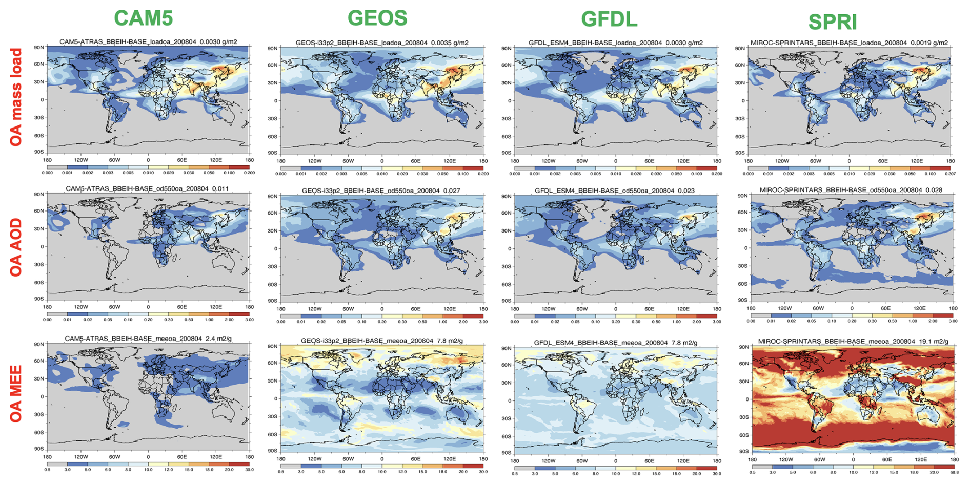
Figure A2 Spatial distribution of OA mass load (units: g m⁻²), OA AOD, OA mass extinction efficiency (MEE) (units: m² g⁻¹) for April 2008, as simulated by four models (CAM5, GEOS, GFDL, and SPRI) in their BASE runs.