Airborne observations of cloud properties during their evolution from organized streets to isotropic cloud structures along an Arctic cold-air outbreak

This case study explores the evolution of clouds during an Arctic cold-air outbreak in the Fram Strait region observed during the HALO–(𝒜𝒞)³ aircraft campaign. Our research provides information about the formation, structure, microphysical and macrophysical properties, and radiative effects and investigates the role of vertical wind shear and buoyancy forces in the transition from regular cloud streets to rather isotropic cloud patterns. Our findings show that lower horizontal boundary layer wind speeds (<12 m s⁻¹) disrupt the formation of cloud streets, leading to more isotropic cloud patterns, characterized by increasing cloud fraction (from 0.73 to 0.84) and cloud top height (from 330 to 390 m), and quantify the increase in liquid water path as well. In addition, we observe an increase in the number concentration of ice crystals in a size range between 100–1000 µm and notable riming processes within organized cloud streets. Concurrent radiation measurements in our case study reveal that isotropic cloud patterns can exhibit either low or high albedo as well as low or high F_net,TIR, suggesting that these patterns represent different developing stages.

1 Introduction

Cold-air outbreaks (CAOs)¹ in the Arctic, which defined by cold air masses moving from the cold sea ice to the warmer ocean, contribute to the increased formation of atmospheric boundary layer (ABL) clouds over the Arctic ocean surfaces. These low-level clouds significantly impact the surface radiative energy budget and can enforce Arctic amplification in winter seasons depending on their macrophysical and microphysical properties such as cloud fraction (Brümmer, 1996; Wendisch et al., 2023; Murray-Watson et al., 2023). However, Brümmer and Pohlmann (2000) have shown that almost any cloud in CAOs over the Greenland Sea and the Barents Sea is strongly inhomogeneous and associated with organized convective patterns in the cloud field. In the initial state of the CAO close to the sea ice, clouds appear in the cloud streets form and often transform into mesoscale cellular cloud patterns some 100 kilometers downstream. These cloud structures change their microphysical, macrophysical, and radiative properties during their evolution (Kirbus et al., 2024; Seppala et al., 2025).

Previous studies have investigated the dynamic characteristics of CAOs, focusing on how ABL processes such as wind shear, buoyancy forces, and turbulence contribute to the formation and evolution of cloud streets (Fletcher et al., 2016). In an early numerical study with a 2D model that does not explicitly resolve turbulence, Etling and Raasch (1987) investigated the development of cloud streets by boundary layer rolls in CAOs. They showed that the inflection point instability, often discussed as a reason for boundary layer rolls in theoretical studies, does not explain the typical cloud structure. Rather, a combination of dynamic and thermal instability was found to cause the formation of rolls. This criterion can be expressed by the ratio of production of turbulent kinetic energy (TKE) by buoyancy (caused by surface heat flux) and vertical wind shear. This simplified view was extended by Gryschka and Raasch (2005) using advanced (3D) large eddy simulation (LES) with a stationary model domain large enough to capture the evolution of the large-scale organized structures, while at the same time the small-scale unorganized turbulence was explicitly resolved. They could confirm that the formation of cloud streets works efficiently for a stability parameter $-H/L<\mathrm{10}$, also called the free roll convection. Herein, H is the top of the ABL, and L is the Monin–Obukhov stability length, which characterizes the relative influence of buoyancy and shear on turbulence generation. The smaller the value, the more TKE production in the ABL is dominated by shear rather than by buoyancy. In fact, $-H/L$ is widely used as a predictor of ABL rolls for various situations, as several observational and numerical studies found clear signals of rolls only for $-H/L<\mathrm{15}$ (e.g. Etling and Brown, 1993). However, in CAO situations, extremely large values of $-H/L$ up to 250 have frequently been observed in cloud street environments (e.g. Brümmer and Pohlmann, 2000). Gryschka et al. (2008, 2014) concluded that this discrepancy is triggered by strong heterogeneities of surface temperatures in the marginal ice zone, also called forced roll convections. In reality, both free and forced roll convection can lead to the formation of cloud streets and cause a high variability in cloud street structure in CAOs, the structure of sea ice, and the magnitude of surface heat flux. To summarize, reasons for roll convection are controversially discussed in the literature, and classical theoretical mechanisms for roll generation do not explain rolls in several CAO situations.

This paper aims at providing an observational proof for the roll convection formation criteria by analyzing airborne observations collected during the HALO–(𝒜𝒞)³ aircraft campaign, which was conducted in March and April 2022 within the framework of the Transregional Collaborative Research Center called “Arctic Amplification: Climate Relevant Atmospheric and Surface Processes, and Feedback Mechanisms” ((𝒜𝒞)³). The flight strategy during HALO–(𝒜𝒞)³ provides repeated observations of CAOs at different times during a flight. Thus, the collected data allow us to analyze the temporal evolution of clouds forming in CAOs.

In Sect. 2, we introduce the instruments and measurement techniques used during the HALO–(𝒜𝒞)³ campaign and present a case study where a transition from clouds with distinct rolls into a more isotropic cloud structure was observed on 4 April 2022. Section 3 outlines the method to quantify the presence of cloud streets and cloud organization and estimates cloud fraction. In Sect. 4, we analyze changes in cloud transitions and link them to cloud macrophysical and microphysical properties, as well as the radiation energy budget. Section 5 explores the dynamic causes of these transitions by analyzing the $-H/L$ stability parameter. Finally, Sect. 6 summarizes the results and provides some conclusions.

2 Measurements and instruments

2.1 HALO–(𝒜𝒞)³ aircraft campaign

During the HALO–(𝒜𝒞)³ campaign, remote sensing and in situ measurements were obtained using instrumentation mounted on three research aircraft: High Altitude and LOng Range Research Aircraft (HALO; Stevens et al., 2019), Polar 5, and Polar 6 (Wesche et al., 2016). Here, we briefly describe those instruments that measure the parameters crucial for this study.

All applied instruments were introduced by Ehrlich et al. (2024). HALO and Polar 5 were equipped with remote sensing instruments and dropsonde launch facilities, while Polar 6 performed in situ measurements (Wendisch et al., 2024). We focus on observations from the Polar 5 aircraft, which mainly operated remote sensing instruments such as a radar, lidar, microwave radiometer, and imaging spectrometer.

Polar 5 was equipped with a digital RGB camera (Nikon D5) with a 180° fish-eye lens for measuring the directional distribution of upward radiance over the lower hemisphere. The images are used for characterizing the horizontal structure of cloud tops and surface conditions every 10 s (Carlsen et al., 2020; Mech et al., 2022). For flight altitudes at 1000 m above cloud top, the pixel size in cloud altitude is about 3.30 m in the image center. The swath, covering 80° of the field of view (FOV), amounts to 1680 m.

Polar 5 and HALO launched dropsondes during flights to measure vertical profiles of air temperature, humidity, pressure, and the horizontal wind vector (George et al., 2021, 2023). HALO released the dropsondes from an altitude of approximately 10 km, while Polar 5 typically deployed them from around 3 km, effectively covering the ABL from both altitudes. The dropsonde measurements have a vertical resolution of 5 m within the altitude range below 1000 m and are of the Vaisala RD41 type, which have an uncertainty of 0.2 K for temperature measurements and 3 % for relative air humidity. The horizontal wind speed accuracy is approximately 0.5 m s⁻¹, with a resolution of 0.01 m s⁻¹. This accuracy is consistent across wind speeds ranging from 0 to 200 m s⁻¹, leveraging Global Positioning System (GPS) technology for wind component measurements (Earth Observing Laboratory, 2023; Vaisala, 2020). It is shown by Ehrlich et al. (2024) that the dropsondes released from HALO and Polar 5 complement each other. While dropsondes launched from HALO provide a broader coverage, the Polar 5 dropsondes improve the spatial resolution, particularly in the Marginal sea Ice Zone (MIZ).

Broadband irradiances, both upward and downward, are measured on Polar 5 using pairs of CMP22 pyranometers and CGR4 pyrgeometers (Becker et al., 2023a). The pyranometers are sensitive for wavelengths ranging from 0.2 to 3.6 µm, while the pyrgeometers cover the thermal-infrared wavelengths between 4.5–42 µm. These measurements are taken at a frequency of 20 Hz, with a sensor uncertainty below 3 % (Gröbner et al., 2014). To correct for the misalignment of the irradiance sensor with respect to a horizontal reference plane during flight concerning downward direct solar irradiance, correction methods from Bannehr and Schwiesow (1993) and Boers et al. (1998) are utilized.

Broadband solar (F_net,sol) and thermal-infrared (F_net,TIR) net irradiances are calculated from the upward and downward irradiances:

$$\begin{array}{}\text{(1)}& {\displaystyle }& {\displaystyle }{F}_{\text{net,sol}}=F_{\text{sol}}^{\downarrow }-F_{\text{sol}}^{\uparrow },\text{(2)}& {\displaystyle }& {\displaystyle }{F}_{\text{net,TIR}}=F_{\text{TIR}}^{\downarrow }-F_{\text{TIR}}^{\uparrow }.\end{array}$$

To mitigate the dependence of F_net,sol on solar zenith angle, which dominates the variation of F_net,sol, a normalization is applied by calculating the cloud albedo:

$$\begin{array}{}\text{(3)}& {\displaystyle }{\displaystyle }\mathit{\alpha }=\mathrm{1}-{\displaystyle \frac{F_{\text{net,sol}}}{F_{\text{sol}}^{\downarrow }}},\end{array}$$

where α denotes the albedo, representing the fraction of incident solar radiation that is reflected.

On Polar 5, thermal-infrared radiance in the nadir direction (field of view 2.3°) is measured using a KT19 infrared pyrometer (model KT19.85 II). The KT19 measurements, with a sampling frequency of 20 Hz, are part of the broadband radiometer dataset (Becker et al., 2023a). Data are provided as brightness temperatures corresponding to the spectral range of the radiometer, covering a narrow wavelength band between 9.6–11.5 µm. These measurements are also used to estimate the sea surface temperature, leveraging the high temporal resolution and spectral sensitivity of the KT19.

The Airborne Mobile Aerosol Lidar (AMALi) on Polar 5 provides profiles of backscatter ratio at two wavelengths (532 and 1064 nm). The data are used to determine the vertical structure of cloud layers, with cloud top altitude as a key measured parameter, having an accuracy of roughly 7 m (Mech et al., 2022; Schirmacher et al., 2023).

The Humidity And Temperature PROfiler (HATPRO; Rose et al., 2005) is part of the instrumentation aboard Polar 5. HATPRO provides brightness temperatures across 14 channels, with half of these channels vertically polarized at the water vapor absorption line at 22.24 GHz (K-band), and the other half are horizontally polarized around the oxygen absorption complex at 60 GHz (V-band; Ehrlich et al., 2024). The processing method for the data obtained from HATPRO is described in detail by Mech et al. (2022). To retrieve the liquid water path (LWP) over the ocean, differences in brightness temperatures between cloud-free and cloudy conditions are utilized following a regression method outlined by Ruiz-Donoso et al. (2020). This method ensures an absolute accuracy of below 30 g m⁻² with a sensitivity below 5 g m⁻² (Ruiz-Donoso et al., 2020; Schirmacher et al., 2024).

The Polar 6 aircraft was equipped with a range of in situ instruments measuring aerosol and cloud particle properties, as well as trace gas and aerosol particle chemical composition. For this study, we focus exclusively on measurements from the Cloud Imaging Probe (CIP) and the Precipitation Imaging Probe (PIP; Wendisch and Brenguier, 2013). These instruments, when used in combination, provide cloud particle size distributions for diameters ranging from 15 µm to 6.4 mm, with resolutions of 15 and 100 µm, respectively. Additionally, both the CIP and PIP capture two-dimensional shadow images of the sampled particles to identify particle phase and shape (Klingebiel et al., 2015, 2023; Moser et al., 2023; Ehrlich et al., 2024).

2.2 Case study: temporal evolution of cloud streets observed during a cold-air outbreak on 4 April 2022

During the HALO–(𝒜𝒞)³ campaign, on 4 April 2022, a distinct CAO was sampled with Polar 5 by a series of overpasses, which were aligned perpendicular to the main wind direction. During this research flight, the dropsonde (DS) location (79.1218° N, 3.0574° E) in the center of the CAO (marked with DS in Fig. 1) was passed four times at approximately 40 min intervals. Each time Polar 5 passed this DS location, a dropsonde was launched to capture vertical profiles of air temperature, humidity, and wind. In addition, HALO launched a dropsonde at the DS location 2 min after the final dropsonde from Polar 5. This repeated observation allows for a detailed analysis of the temporal evolution of the cloud streets into isotropic cloud structures over an extended period. Waypoint 1 (WP1) and Waypoint 2 (WP2) in Fig. 1 were selected based on the flight track to define the section where Polar 5 and Polar 6 repeatedly flew back and forth to observe the temporal evolution of cloud properties. While some dropsondes were deployed near WP1 and WP2 (as marked in Fig. 1), these were not included in our analysis. Instead, we focus on the dropsondes released at the DS location, where the cloud transitions were most clearly observed.

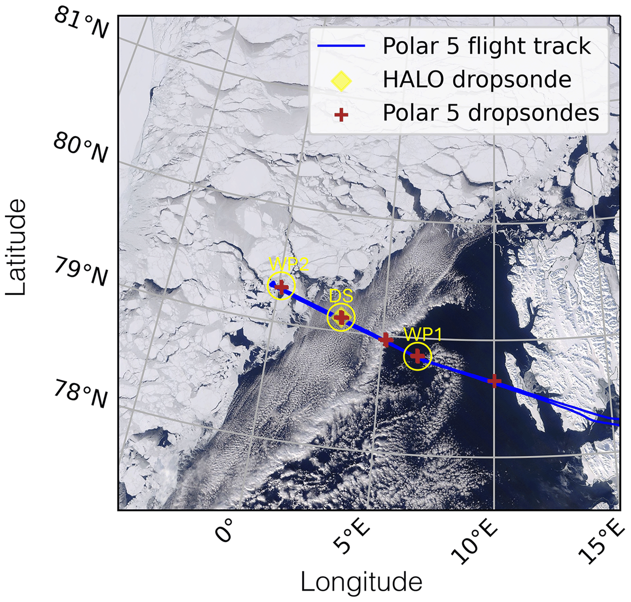
Figure 1 Flight track of Polar 5 on 4 April 2022. The red crosses and the yellow diamond mark the locations of the dropsondes from Polar 5 and HALO, respectively. The satellite picture is a composite snapshot from NASA Worldview (MODIS) of that day (https://worldview.earthdata.nasa.gov, last access: 18 October 2023). The yellow circles indicate waypoint 1 (WP1) and WP2, as well as the dropsonde (DS) location (79.1218° N, 3.0574° E).

On 4 April 2022, the weather conditions in the Fram Strait were part of a broader cold period following a significant shift from warm conditions in late March. This period, characterized by CAOs, began on 21 March 2022 and lasted until 12 April 2022 (Walbröl et al., 2024). To illustrate the flight operations on that day, Fig. 1 shows the flight track of Polar 5 along with the locations where dropsondes were deployed.

3 Methods to derive cloud street index and cloud fraction

To quantify the intensity of the cloud street structure along the flight leg, we develop in this section an index, which describes that. In addition, we explain how we derive the cloud fraction, based on the fish-eye camera images.

Figure 2a and d show two examples of RGB images from the fish-eye camera that illustrate two different cloud regimes. The image in Fig. 2a shows an organized cloud street, while the later image, in Fig. 2d, represents clouds with a more random pattern. These two types of cloud structures will be referred as cloud streets and as isotropic cloud patterns in the following. To quantify cloud organization during CAOs and analyze its impact on radiative properties, cloud dynamics, and transitions to isotropic cloud patterns, the color images were first converted to grayscale units. Figure 2b and c show grayscale values in along-track and across-track directions (gray lines) with Polar 5 flying perpendicular to the cloud rolls. To identify cloud rolls, the moving average, with a windows size of 20 pixels, of each line was calculated. Local maxima of the along-track, n_lt, and across-track, n_ct, directions were identified (dots), and the numbers of local maxima were counted for both directions. The ratio of the number of maxima in both directions, which we introduce as the cloud street index, I_CS, is calculated by the following formula:

$$\begin{array}{}\text{(4)}& {\displaystyle }{\displaystyle }{I}_{\text{CS}}=\mathrm{1}-{\displaystyle \frac{n_{\text{lt}}}{n_{\text{ct}}}}.\end{array}$$

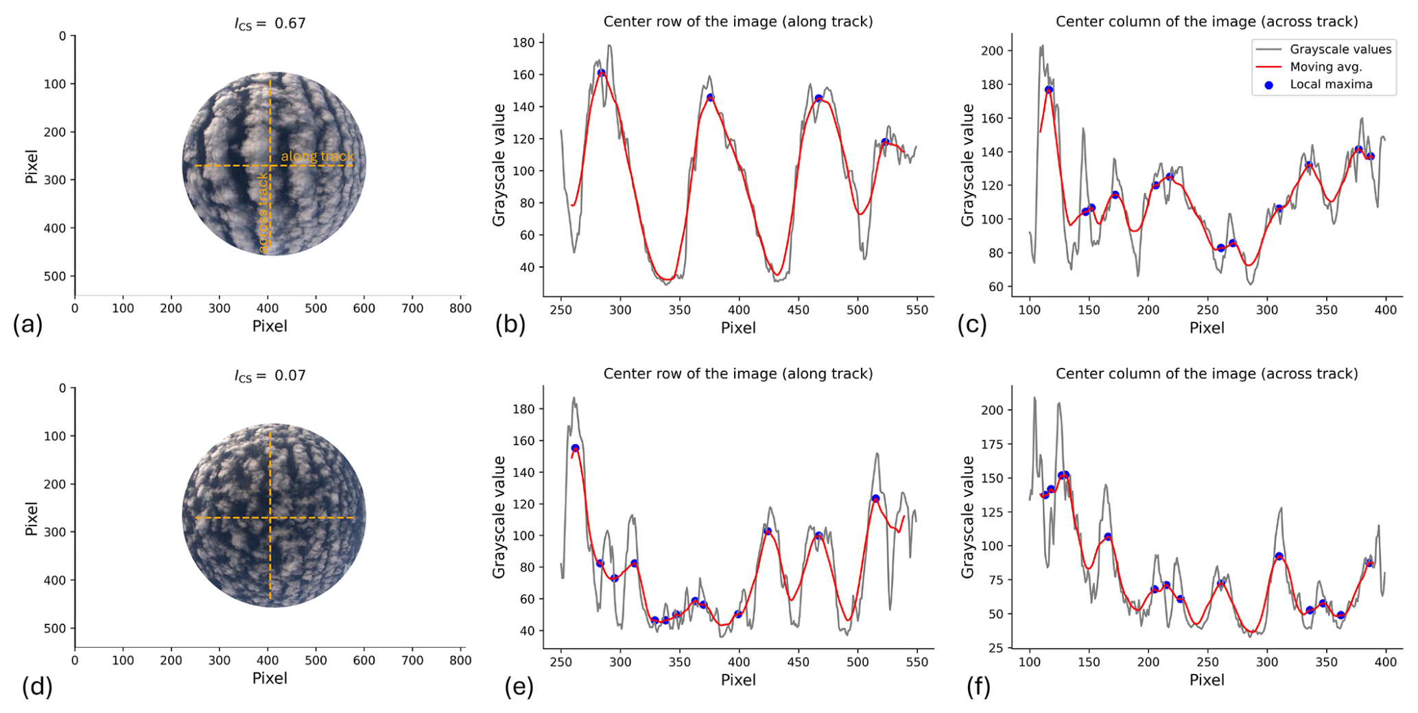
Figure 2 Estimation of the cloud street index, I_CS, in different cloud situations: panels (a) to (c) illustrate the method applied to a cloud street case, while panels (d) to (f) show its application to isotropic cloud patterns. In the fish-eye camera images in (a) and (d), the orange dashed lines represent the cross sections where the identification method was applied. Panels (b), (c), (e), and (f) display the grayscale pixel values along the horizontal (b and e) and vertical (c and f) cross sections. The gray lines indicate these grayscale values, and the red lines represent their moving averages, with the local maxima marked by blue dots.

High values of I_CS indicate a more pronounced organization of the clouds into cloud streets, while low values of I_CS characterize isotropic cloud patterns.

For the cloud street case depicted in Fig. 2a, 4 maxima (n_lt=4) were identified in the along-track direction (Fig. 2b), and 12 maxima (n_ct=12) are present in the across-track direction (Fig. 2c), resulting in I_CS=0.67 for an organized cloud street structure. For the isotropic cloud pattern, I_CS is 0.07 (13 maxima in the horizontal direction and 14 in the vertical direction).

This method was developed for the specific case study and may require modification for larger datasets, particularly if the flight pattern was not perpendicular to the direction of the cloud streets or the clouds streets change in their dimension.

The cloud fraction is estimated using images captured by the fish-eye camera at 10 s intervals. In a first step, these images are dewarped, as presented in Fig. 3a. Cloud pixels were identified based on the ratio of the red and blue channels, as clouds generally exhibit higher reflectance in the red spectrum compared to the blue. A threshold of 0.8 was chosen based on visual inspection of multiple images to ensure accurate cloud detection. The resulting image, showing the identified clouds, is displayed in Fig. 3b. Figure 3c illustrates the distribution of the ratio of the red and blue channels, indicating the applied threshold (dashed line). For our following case study, this simple approach is sufficient. However, applying this method to a dataset with a lower solar zenith angle would require a more sophisticated approach to avoid phenomena such as sun glint and sea ice patches, which affect the performance of this cloud fraction retrieval. It should be noted, since the fish-eye camera images are taken at an oblique angle, that the derived cloud fraction may be slightly overestimated compared to a nadir view, especially for thicker clouds. In addition, because the images are taken every 10 s, they partially overlap, meaning that some cloud structures may appear in multiple images. However, since the aircraft is continuously moving forward, each image still captures a new portion of the cloud field, and the overlap does not significantly impact the cloud fraction determination. These effects should be considered when interpreting the cloud fraction results.

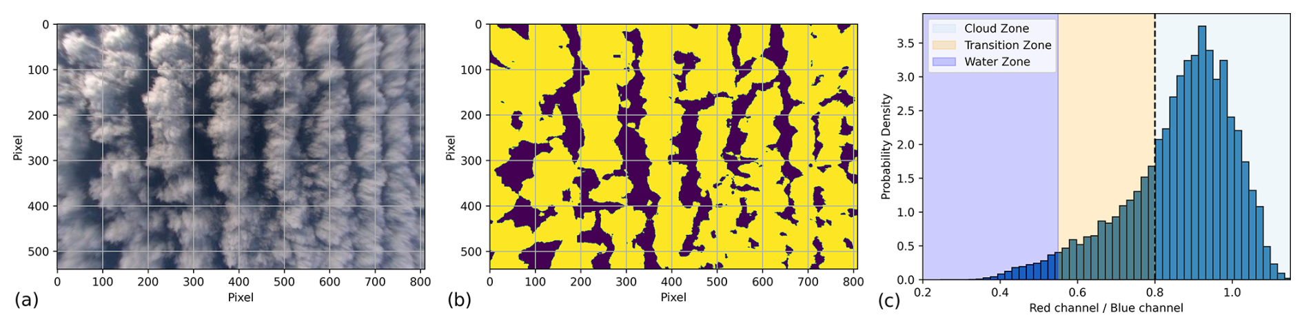
Figure 3 Estimation of the cloud fraction based on fish-eye camera images. Panel (a) shows the dewarped image of cloud streets captured by the fish-eye camera mounted at the fuselage of Polar 5. Panel (b) presents the applied cloud mask to the image. The cloud fraction based on this mask is here 0.73. Panel (c) displays the ratio of the red and blue channel, indicating the distribution of pixels from clouds and the water surface inside the image. The dashed line indicates the threshold of 0.8, which was used to separate between cloud and cloud-free areas.

4 Changes of cloud and radiation properties during transition

To identify how the cloud and radiation properties are changing during the transition from cloud streets to isotropic cloud patterns, we focus in this section on the flight leg between WP1 and WP2 (see Fig. 1). For the analysis of cloud properties and organization, only data west of 5.0° E were considered to exclude unrelated cloud structures (e.g. the cloud band, which is visible in Fig. 1) outside the main region of interest.

4.1 Macrophysical cloud property changes

The cloud fraction decreases from 0.84 to 0.73 with an increasing I_CS (Fig. 4a), which is expected since a high I_CS indicates more-intense roll clouds with more-pronounced cloud-free areas. This trend is likely due to the cloud organization in linear structures, which creates cloud-free zones between the cloud streets. This reduces the overall cloud fraction, which is particular important because cloud fraction plays an important role in the radiation budget (Feingold et al., 2017). Larger cloud-free regions allow for more solar radiation to reach the surface, while a higher cloud fraction reflects more solar radiation and therefore leads to a cooling of the surface during polar day.

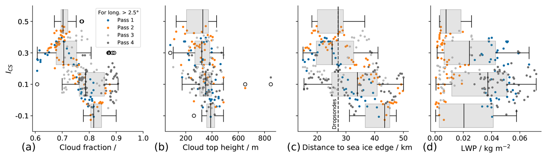
Figure 4 The panels show cloud fraction (a), cloud top height (b), distance to sea ice edge (c) with the location of the dropsondes indicated as dashed line, and the LWP (d) as a function of I_CS. The distribution of the data is presented as box-and-whisker plots.

Cloud top height slightly increases from 330 to 390 m with a decreasing I_CS (Fig. 4b). This trend is likely due to less shear and stronger buoyancy associated with a lower I_CS, which potentially allows clouds to develop vertically and reach higher altitudes. Wind shear in organized cloud street structures inhibits vertical motion and tends to CAO cloud growth, while more isotropic clouds can experience greater convective activity, which results in higher cloud tops.

I_CS decreases with increasing distance to the sea ice edge (Fig. 4c), because the air masses sampled further from the sea ice had more time to evolve over the ocean (Schirmacher et al., 2024). This means that isotropic cloud patterns occur in our study more frequently with increasing distance to the sea ice edge. The spatial distribution of these cloud patterns affects the Arctic radiative energy budget. This spatial variation shows that their radiative impacts are not uniform across different regions, which highlights the importance of accurately modeling cloud structures in CAOs.

The LWP does not show a clear trend with I_CS across all passes, although passes 1 and 4 show higher LWP with lower I_CS (Fig. 4d). However, focusing on pass 1 and 4, it shows that the highest LWP values are reached for small I_CS. This is plausible, because the lower I_CS indicates thicker clouds, which contain more liquid water. These observations suggest that the changes in cloud structure not only affect the cloud macrophysical properties, like cloud top height and cloud fraction, but also influence the microphysical characteristics of the clouds, such as the droplet size distribution (see also Sect. 4.2) and LWP.

All in all, the changes in cloud street structure and the associated consequences on cloud fraction and cloud top height reveal the influence of cloud organization on the Arctic radiation budget close to the surface. As cloud street structures transition to more isotropic cloud patterns, changing cloud macrophysical and microphysical properties affect the energy exchange between the atmosphere and the surface.

4.2 Microphysical changes of large ice particles and riming dynamics

In situ cloud measurements of microphysical properties from Polar 6 are available for passes 2 and 4 of the case study, providing detailed observations of cloud particle distributions at low altitudes. Polar 5 and Polar 6 were well colocated during the flight. Polar 5 flew slightly behind Polar 6 to enable dropsonde deployments without affecting the in situ measurements from Polar 6. As a result, the measurements from both aircraft are directly comparable. The in situ data were sampled at an altitude of approximately 200 m (see Fig. 5a), well below cloud top, which was about 400 m.

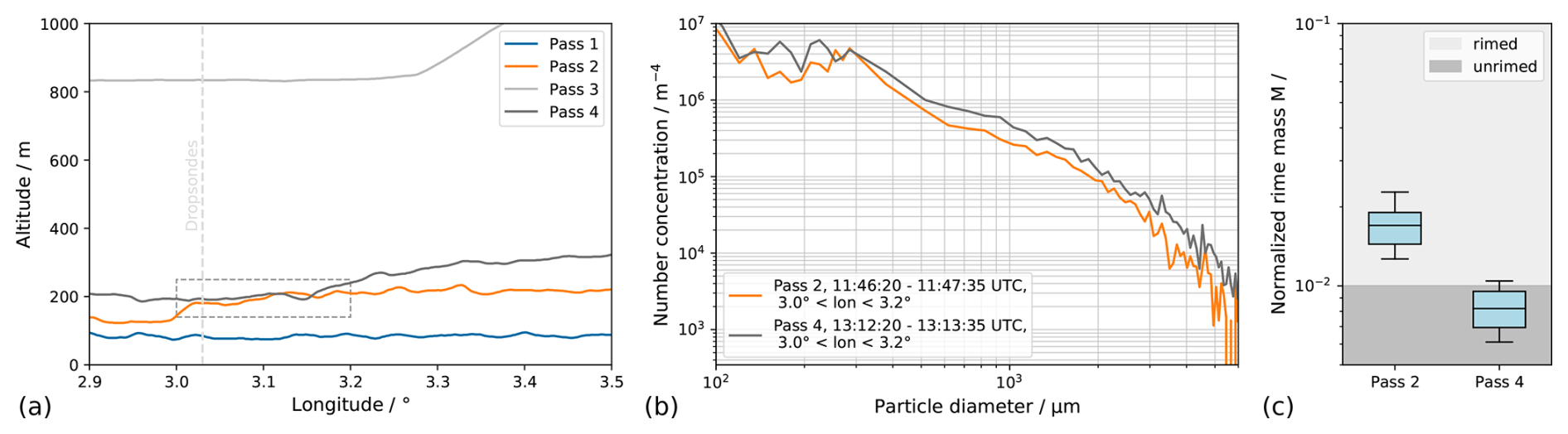
Figure 5 Microphysical cloud particle measurements obtained from the Polar 6 research aircraft. Panel (a) illustrates the flight paths of Polar 6, highlighting the overlapping sampling region during passes 2 and 4, as indicated by the box, and the DS location (location of the dropsondes), as indicated by the dashed line. The corresponding size distributions for this area are presented in (b). Panel (c) shows boxplots of the normalized rime mass for both passes along the flight leg, indicating the threshold between rimed and unrimed particles.

Figure 5b presents the number size distributions of cloud particles in the range from 100 to 6000 µm averaged for passes 2 and 4. It is evident that during pass 4 the particle concentration was higher across almost the entire size range. The higher particle concentration of pass 4 along the flight leg is the result of the higher ABL and higher cloud top heights, which supports the growth of cloud particles. These characteristics suggest deeper clouds, where larger ice particles can form and precipitate. In addition, the presence of more large particles during pass 4 might also indicate aggregation processes, where smaller ice crystals collide and stick together, forming larger ice particles, which might precipitate. This is a typical process for the development of Arctic precipitation (Morrison et al., 2012), especially in cold-air outbreak conditions where ice-phase processes dominate (Schirmacher et al., 2024).

In addition, we investigated the occurrence of riming for pass 2 and pass 4, which describes the accretion of supercooled liquid water onto ice particles. We calculated the normalized rime mass M of ice particles, which is defined as the rime mass divided by the mass of a spherical graupel particle with equal particle size (Seifert et al., 2019). To derive M, we used the in situ method from Maherndl et al. (2024), which is based on in situ observations of particle shape. Only a subset of particles can be used to derive M (particle diameters must be larger than 210 µm for CIP and larger than 1400 µm for PIP), because small particles have round shapes due to imager resolution. For a detailed description of the method and its limitations, we refer the reader to Maherndl et al. (2024). We consider particles with M<0.01 to be unrimed due to their nearly identical scattering properties to particles with M=0 (Maherndl et al., 2023).

We identified a distinction in the riming characteristics between both passes along the flight leg (see Fig. 5c). During pass 2, where the cloud streets are visible, we see that riming is present with a higher median normalized rime mass value of M=0.017. Compared with that, we see during pass 4 (isotropic cloud pattern) a negligible M (0.008), which confirms the absence of riming. Regarding Maherndl et al. (2024), the lack of riming in pass 4 indicates conditions with less favorable dynamics for riming to occur. We assume that the differences in the riming characteristics correlate with the appearance of cloud streets and isotropic cloud patterns. Cloud streets are typically associated with stronger vertical shear at cloud top, while the transition to isotropic cloud patterns coincides with a reduction in wind shear, suggesting a shift toward buoyancy-driven convection. These isotropic cloud patterns contain lower turbulence (lower TKE), which likely reduces riming processes and therefore leads to a lower M.

4.3 Radiation energy budget changes

Figure 4a reveals a strong correlation between I_CS and cloud fraction. It is known that α increases monotonically with cloud fraction (Feingold et al., 2017). Therefore, a relationship between I_CS and α is expected. This correlation is evident in Fig. 6a, where α increases linearly with cloud fraction. Consistent with this, F_net,TIR and cloud fraction show a similar trend, although with higher uncertainty (Fig. 6b).

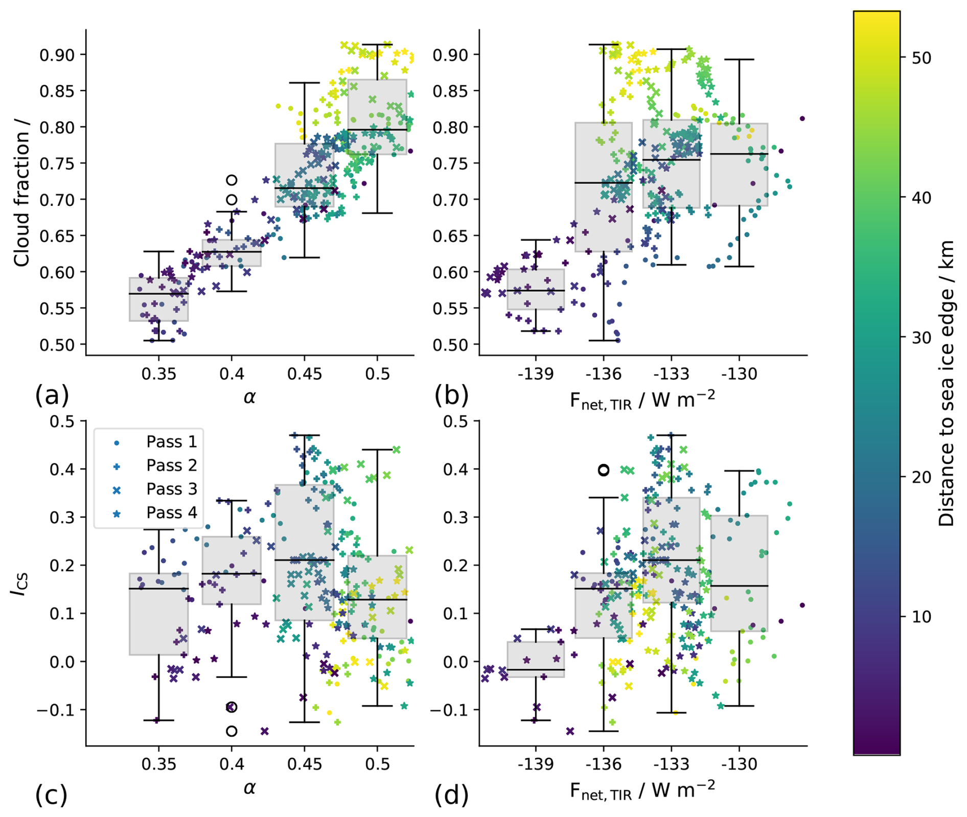
Figure 6 Albedo (α) and F_net,TIR as a function of cloud fraction (a, b). And α and F_net,TIR as a function of I_CS (c, d). The different symbols mark the data sampled at the different passes along the flight leg. The colors indicate the distance to the sea ice edge of the measurements.

Interestingly, a linear trend between α and I_CS is not visible in Fig. 6c. Here, an increase in α with increasing I_CS is noticeable between α=0.35 and α=0.45. For higher α values, I_CS tends to lower values. The colors in Fig. 6c indicate the distance to sea ice, which suggests the presence of two different isotropic cloud regimes: one with a higher α (over the open water) and one with a lower α (near the ice). This shows that the albedo of the isotropic clouds does not depend directly on I_CS. It seems that, depending on the development state, the isotropic cloud patterns (with a low I_CS) can have either low or high α. This theory is also applicable to F_net,TIR in Fig. 6d. The absence of a clear linear trend between α and I_CS in Fig. 6c highlights the complexity of the radiative energy budget during the cloud transition process. The observed nonlinear relationship suggests that other factors might play a role in shaping the cloud patterns and their corresponding radiative properties. It shows that despite having similar I_CS values, isotropic clouds can exhibit a wide range of albedo values, driven by other factors like their varying microphysical properties and developmental states (Bony et al., 2006).

5 Dynamic causes of cloud transition

5.1 The role of the ABL wind speed and $-H/L$

To estimate whether the reduction in ABL wind speed is the primary driver of changes in the cloud street structure, we analyzed the stability parameter and roll predictor $-H/L$ mentioned in the Introduction (Sect. 1). Herein, L is the Obukhov length describing the effect of buoyancy and vertical wind shear on turbulence in the surface layer of the ABL:

$$\begin{array}{}\text{(5)}& {\displaystyle }{\displaystyle }L=-{\displaystyle \frac{{\mathit{\theta }}_{\mathrm{0}}}{\mathit{\kappa }g}}{\displaystyle \frac{(\stackrel{\mathrm{‾}}{w^{\prime }{u}^{\prime }}{)}_{\mathrm{0}}^{\mathrm{3}/\mathrm{2}}}{(\stackrel{\mathrm{‾}}{w^{\prime }{\mathit{\theta }}^{\prime }}{)}_{\mathrm{0}}}},\end{array}$$

with θ₀ a reference potential temperature in the surface layer, g the gravitational acceleration, κ=0.4 the von Kármán constant, and $(\stackrel{\mathrm{‾}}{w^{\prime }{u}^{\prime }}{)}_{\mathrm{0}}$ and $(\stackrel{\mathrm{‾}}{w^{\prime }{\mathit{\theta }}^{\prime }}{)}_{\mathrm{0}}$ the mean near surface turbulent fluxes of momentum and temperature, respectively. To estimate this length scale with the dropsonde measurements, we followed the approach in Brümmer (1999) and calculated the fluxes with the bulk aerodynamic formulas:

$$\begin{array}{}\text{(6)}& {\displaystyle }& {\displaystyle }(\stackrel{\mathrm{‾}}{w^{\prime }{u}^{\prime }}{)}_{\mathrm{0}}=C_{\mathrm{D}}{U}_{\mathrm{90}}^{\mathrm{2}},\text{(7)}& {\displaystyle }& {\displaystyle }(\stackrel{\mathrm{‾}}{w^{\prime }{\mathit{\theta }}^{\prime }}{)}_{\mathrm{0}}=C_{\mathrm{H}}\mathrm{\Delta }{\mathit{\theta }}_{\text{as}}{U}_{\mathrm{90}}.\end{array}$$

Herein, U₉₀ is the 90 m wind speed, Δθ_as the potential temperature difference between the air at 90 m height and the water surface, and C_D and C_H the dimensionless drag and heat transfer coefficients. Dropsonde data for U₉₀ and air temperature were taken from the 90 m level to ensure reliability, given the 5 m vertical resolution of the measurements (as detailed in Sect. 2) and to minimize uncertainties associated with the lowest few meters above the surface. Thus, the stability parameter $-H/L$ can be written in the form

$$\begin{array}{}\text{(8)}& {\displaystyle }{\displaystyle }-H/L=H{\displaystyle \frac{\mathit{\kappa }g}{{\mathit{\theta }}_{\mathrm{0}}}}{\displaystyle \frac{C_{\mathrm{H}}\mathrm{\Delta }{\mathit{\theta }}_{\text{as}}{U}_{\mathrm{90}}}{{\left(C_{\mathrm{D}}{U}_{\mathrm{90}}^{\mathrm{2}}\right)}^{\mathrm{3}/\mathrm{2}}}}.\end{array}$$

Similarly to Brümmer (1999), we assumed the drag and transfer coefficients to be equal as $C_{\mathrm{D}}=C_{\mathrm{H}}=\mathrm{1},\mathrm{3}\times {\mathrm{10}}^{-\mathrm{3}}$.

Table 1 Cloud street index I_cs and stability parameter $-H/L$ calculated with Eq. (8) and corresponding values for U₉₀ as well as further values mentioned in the text during the research flight on 4 April 2022.

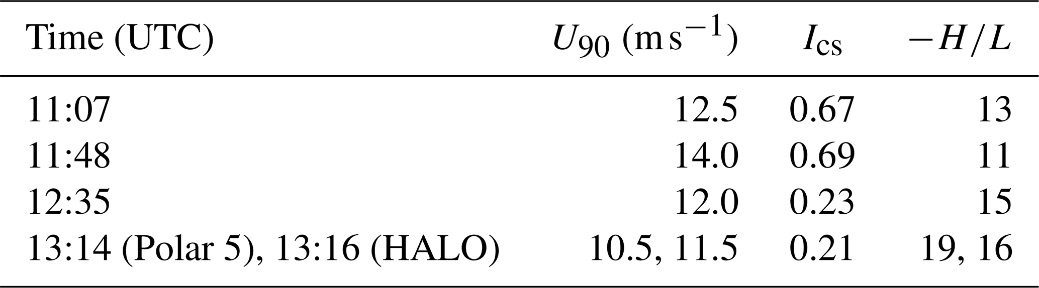
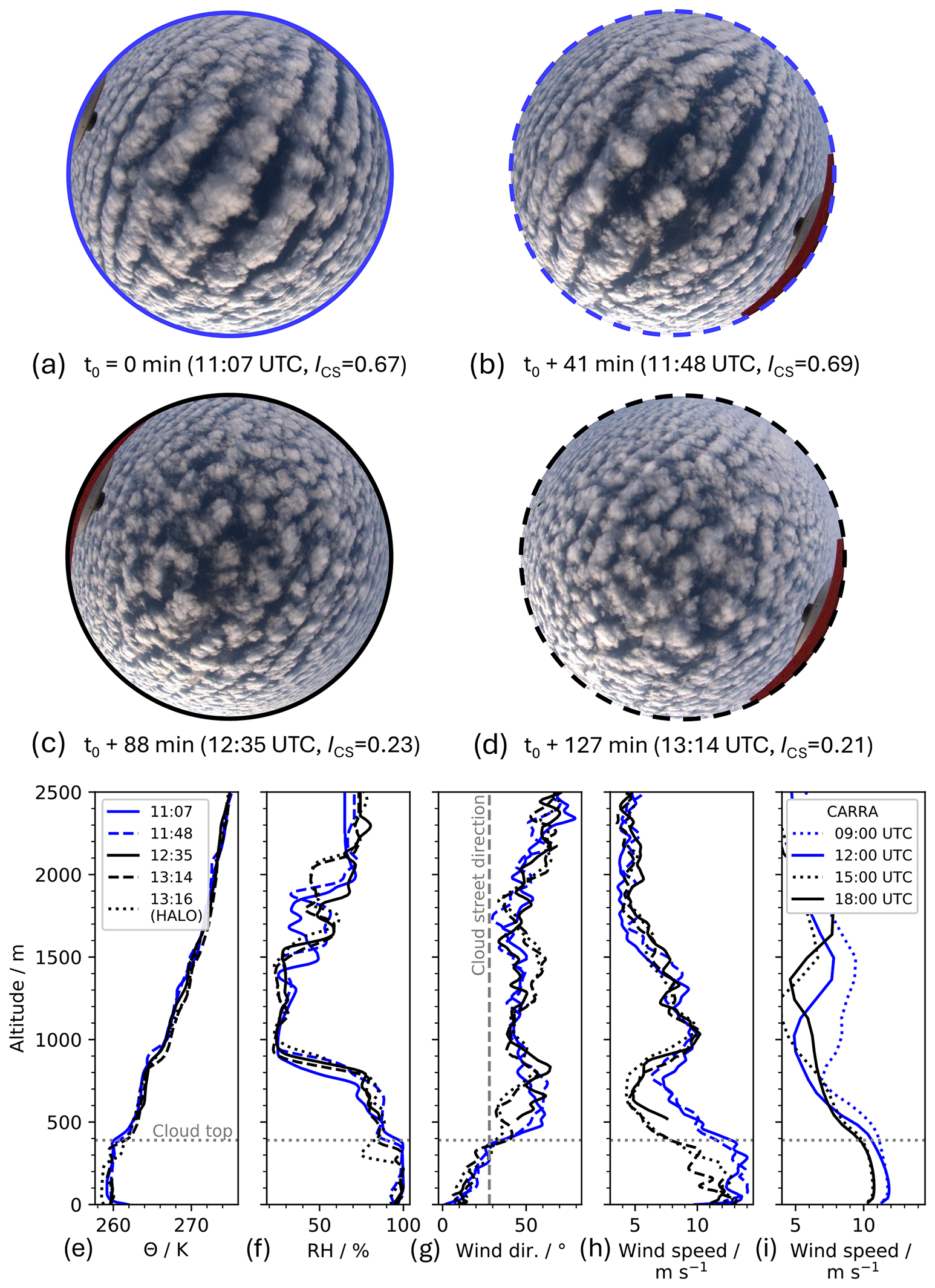
Figure 7 (a–d) Fish-eye camera images taken at the DS location (marked with DS in Fig. 1) during the Polar 5 flight on 4 April 2022. The top of each image is aligned towards north, and the cloud street index, I_CS, is indicated. (e–h) Vertical profiles from HALO (dotted) and Polar 5 dropsondes (dashed and solid) of potential temperature, relative humidity, wind direction, and wind speed at the DS location where the fish-eye camera images were taken. The dotted horizontal line indicates the cloud top height, and the vertical dashed line in (g) represents the direction of the cloud streets. Note that the dropsonde launched at 12:35 UTC lacks data below an altitude of 500 m. (i) Vertical profiles of Copernicus Arctic Regional Reanalysis (CARRA) data at the previously mentioned DS location for different times.

Table 1 compares the cloud street index I_cs and $-H/L$ during the Polar 5 flight on 4 April 2022 at different times at the DS location marked in Fig. 1. $-H/L$ was calculated with Eq. (8) using Polar 5 dropsondes (see Fig. 7), and the sea surface temperature was estimated with KT19 measurements. We used the values H=400 m, θ₀=260 K (which also equal the temperature of the mixed layer as the 90 m temperature), and Δθ_as=12.5 K for a sea surface temperature of 272.5 K. Although these values are almost constant during the period studied, the values for U₉₀ vary in time and therefore are given in Table 1 for different times. Clear signals of cloud streets appeared in the cloud street index I_cs from 11:07 UTC to 11:48 UTC with values for $-H/L$ less than 15. From 12:35 UTC, a breakup in cloud streets can be identified by a significant decrease in I_cs from values around 0.7 to values around 0.2, accompanied by an increasing stability parameter ($-H/L\ge \mathrm{15}$). The breakup can also be seen by eye in the camera images in Fig. 7a–d. This behavior fits to the discussion on the critical value of around 15 for $-H/L$ in Etling and Brown (1993), mentioned in Sect. 1. According to Gryschka et al. (2008, 2014) and the discussion in Sect. 1, the cloud streets observed at position DS between 11:07–11:48 UTC can be attributed to free rolls, which appear due to a pure self organization of the flow. In other words, upstream of position DS surface heterogeneities in the sea ice distribution are not sufficient to force roll convection; otherwise, cloud streets should also be observed for larger values of $-H/L$ as in Brümmer (1999), where cloud streets for values even larger than 200 were reported. We would like to mention that the critical value of 15 for $-H/L$ should not be understood as a switch for free rolls or no free rolls. With increasing values from about 15, the pattern of free rolls can be expected to become more and more unclear.

Beside $-H/L$, the Richardson number Ri is often discussed in the context of boundary layer rolls in observations. It goes back to an early theoretical work of Brown (1972), where with a perturbation analysis of a stratified Ekman boundary layer it was found that boundary layer rolls are most likely when there exists in the vertical wind profile of the cross-roll component an inflection point in the upper part of the ABL, and the local Richardson number (Ri) near the inflection point is below a critical value of 0.25. This so-called inflection point instability could not be confirmed under moderate convective conditions by several numerical studies (e.g. Etling and Raasch, 1987; Gryschka and Raasch, 2005). Regardless, in several experimental studies Ri was linked with different bulk approaches to roll development. Some of these approaches are summarized in Brooks and Rogers (1997). In contrast to Brown (1972), all of these approaches calculate Ri with values of temperature and wind speed over the entire ABL rather than locally at the inflection point. Therefore, it cannot be expected that the theoretical critical value of 0.25 from Brown (1972) can be used for the bulk approach in general. Brooks and Rogers (1997) pointed out that critical values of Ri for roll appearance might need to be adapted to the bulk approach. We also tested some approaches on Ri mentioned in Brooks and Rogers (1997) and found that the values of Ri were very sensitive to the approach. The parameter $-H/L$, originally suggested as roll predictor in one of the first LES studies by Deardorff (1972), seems to be more robust here. It should be borne in mind that all these parameters are defined for idealized profiles of wind and temperature.

We conclude that, in the present case, most likely the reduction in wind speed is responsible for breakup of cloud streets, because other parameters appear to vary less than wind speed. We are aware that the wind speed measured by the dropsondes has a large scattering. Nevertheless, the reduction in wind speed during the breakup can be seen in the entire ABL and not only at 90 m height. Although based on a small sample size, these airborne observations provide the first direct in situ confirmation, to our knowledge, of the theoretical link between decreasing wind speed and the transition from cloud streets to isotropic cloud patterns, as previously suggested by modeling studies (e.g. Gryschka and Raasch, 2005).

5.2 Vertical profiles

Figure 7a–d show images captured by the fish-eye camera, which enables a comprehensive view of the temporal changes in the cloud streets. Alongside these images, Fig. 7e–h present the vertical profiles of potential temperature, θ; relative humidity, RH; wind direction; and wind speed from the dropsonde launches at the DS location.

The fish-eye camera images clearly show that the cloud structure at the DS location changes over time (Fig. 7a–d). Starting with a distinct cloud street formation (Fig. 7a), the structure gradually dissolves into a scattered, isotropic cloud pattern, visible in Fig. 7c and d. By applying the previously defined parameter, I_CS, higher values of 0.67 and 0.69 are obtained for Fig. 7a and b, respectively, and lower values of 0.23 and 0.21 are obtained for Fig. 7c and d.

To investigate the atmospheric changes causing these structural alterations, the vertical profiles from the dropsondes launched at the DS location are shown in Fig. 7e–h. These profiles indicate that θ, RH, and the wind direction remain rather constant over the 2 h period between the first and fourth pass along the flight leg. The cloud top height of 390 m matches the beginning of the inversion layer height. In comparison to other CAO events, which was discussed by Schirmacher et al. (2024) and Walbröl et al. (2024), these cloud tops seem low, which is typical for a weaker CAO. However, in Fig. 7h a noticeable decrease in wind speed is seen, with a wind speed at cloud top approximately 4 m s⁻¹ lower during the last overpass (13:14 UTC with Polar 5 and 13:16 UTC with HALO) compared to the first overpass (11:07 UTC).

This reduction in wind speed seems to be the reason for the transition of the cloud structure, changing from distinct cloud streets to an isotropic cloud pattern.

5.3 Spatial analysis using the CARRA data

The spatially highly resolved Copernicus Arctic Regional Reanalysis (CARRA) data result from the HARMONIE-AROME non-hydrostatic regional numerical weather prediction model (Bengtsson et al., 2017; Schyberg et al., 2020), which are available for two domains that overlap in the vicinity of Svalbard (Schyberg et al., 2020; Kirbus et al., 2024). CARRA-West covers Greenland, while CARRA-East covers Svalbard and northern Scandinavia. The temporal resolution of CARRA data is 3 h with a horizontal grid resolution of 2.5 km on 65 vertical model levels (from 15 m up to about 26 km) and 20 vertical model levels below 1000 m altitude.

In Sect. 5.1, we elaborated that a decrease in wind speed below 12 m s⁻¹ leads to a breakup of the cloud street structures. To identify how the wind speed changed spatially, we present in Fig. 8 the wind speed field for four different times, at an altitude of 90 m, in the vicinity of the flight track. It is visible that at the DS location (marked by DS) the wind speed decreases between 09:00 UTC (Fig. 8a) and 18:00 UTC (Fig. 8d). In addition, it is noticeable that the Lee region, southwest of Svalbard with wind speeds below 8 m s⁻¹, is shifting further west.

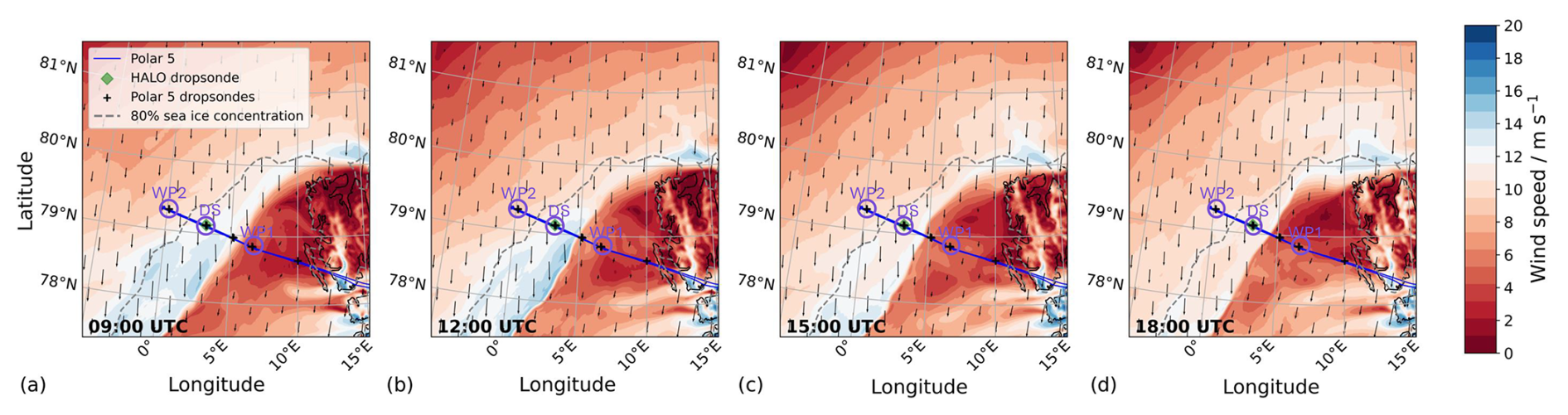
Figure 8 CARRA wind field on 4 April 2022 at an altitude of 90 m for different time steps (a–d). Each time step shows the flight track of Polar 5. The circles mark waypoints (WP) 1 and 2 and the dropsonde region of interest (DS). The location of the dropsonde launches from HALO and Polar 5 are indicated by the diamond and the crosses, respectively. AMSR2 data (Meier et al., 2018), which show the sea ice edge with a sea ice concentration of 80 %, are indicated by the dashed gray line. The arrows indicate the wind speed and wind direction at cloud top altitude.

To identify how the vertical wind speed in CARRA data compares to the measured dropsonde profiles, we show in Fig. 7i the altitude profiles of CARRA at the closest grid point to the DS location (approximately 360 m distance). It is visible that between 12:00–15:00 UTC the wind speed at cloud top decreases from about 11.5 to 10 m s⁻¹. Although this change is less compared to the dropsonde profiles (13–8 m s⁻¹) in Fig. 7h, the reanalysis data also show a decrease through the whole ABL.

6 Summary and conclusions

In the presented case study, we analyze the evolution of clouds during a CAO event observed on 4 April 2022, focusing on the transition from organized cloud streets to isotropic cloud patterns. While previous studies of Arctic CAOs have focused on their distinct roll cloud convection patterns, this study examines the temporal evolution of cloud street structures. The research aircraft Polar 5 flew a path perpendicular to the cloud street direction, repeatedly launching dropsondes at the same location. The clouds below the flight path were sampled four times as Polar 5 flew back and forth. Five dropsondes were launched in the center of the CAO, capturing the vertical atmospheric profile. Fish-eye lens images from a camera mounted at the bottom of the Polar 5 fuselage showed a transformation of clouds from a distinct cloud street pattern to a more isotropic cloud pattern over 127 min.

To estimate changes of the cloud street structure, we introduced the cloud street index. Combined with remote sensing observations from the aircraft, the index provides a quantitative measure to evaluate the cloud structure, macrophysical and microphysical cloud properties, and the radiation budget during the temporal evolution of clouds along CAOs.

A finding of this case study is that decreasing wind speed drives the transition from organized cloud streets to isotropic cloud patterns. The link between wind speed and the transition of cloud structure is quantified using the $-H/L$ stability parameter, which measures the relative importance of vertical wind shear (which promotes turbulence and organized convection) and buoyancy (which drives vertical mixing). For $-H/L<\mathrm{15}$, turbulence generated by wind shear dominates, favoring the formation of organized cloud streets. However, as $-H/L$ increases beyond this threshold, buoyancy becomes increasingly significant, and the organized cloud streets collapse into more isotropic cloud patterns. In our case study, the reduction in wind speed is the dominant factor increasing $-H/L$, disrupting the organized convection which is required to sustain cloud streets. While this finding is based on a single case study, it provides valuable observational support for theoretical and modeling studies that propose wind shear as a critical factor in maintaining cloud street organization and consequences for cloud microphysical and radiative properties.

Our analysis of the cloud microphysics revealed increased concentrations of larger cloud ice particles for the isotropic cloud patterns than for the organized cloud street structures. This transition also marked significant changes in the riming dynamics. For the cloud street structures, riming – a process where supercooled liquid water accretes onto ice particles – was present with a higher normalized rime mass (M=0.017). Conversely, riming was negligible (M=0.008) for the isotropic cloud patterns, which indicates reduced turbulence and weaker shear forces. Our findings suggest that cloud streets, characterized by higher turbulence and shear, promote riming, whereas isotropic cloud patterns are more buoyancy driven and exhibit lower riming activity. In terms of the surface radiation budget, isotropic cloud patterns (with low I_CS) exhibit either a low or high α and a low or high F_net,TIR. In our case study, this suggests the presence of two different isotropic cloud regimes, which seem to be at different developing stages. Therefore, a linear correlation between α and I_CS is not recognizable.

In conclusion, this case study shows that cloud streets initiated by Arctic CAOs can change their cloud structure due to minor environmental changes, which then can affect cloud microphysics and macrophysics and the radiation budget. Cloud-resolved numerical modeling, such as LES, is needed to parameterize such transitions of cloud structure as well as their dependencies.