Moisture budget estimates derived from airborne observations in an Arctic atmospheric river during its dissipation

Atmospheric rivers (ARs) are essential for the Arctic water cycle, but observations quantifying the moisture processes of individual Arctic ARs are sparse. This study quantified the evolution of the moisture budget components of an Arctic AR derived from airborne observations from two research flights on consecutive days. We investigated how poleward transport of warm and moist air masses by ARs generates precipitation near the sea ice edge and how advection and evaporation affect the local moisture amount during the dissipation of the AR. Using observations from the High-Altitude and LOng-Range Research Aircraft (HALO), we derived the atmospheric moisture budget components (local tendency of moisture, evaporation, moisture transport divergence, and precipitation) within an Arctic AR during the HALO-(𝒜𝒞)³ aircraft campaign. The budget components were quantified in sectors ahead of the AR-embedded cold front using airborne observations from dropsondes, radiometers, and a radar device and compared with values derived from reanalyses and numerical weather prediction simulations.

We found that the observed moisture budget components in the pre-cold frontal sectors contribute up to $\pm \mathrm{1}\mathrm{mm}{\mathrm{h}}^{-\mathrm{1}}$ to the local moisture amount. The moisture transport divergence primarily controls the local moisture amount within the AR, while surface interactions are of minor importance. Precipitation is heterogeneous but overall weak ($<\mathrm{0.1}\mathrm{mm}{\mathrm{h}}^{-\mathrm{1}}$), and evaporation is small. As the AR dissipated, the budget components changed from drying to moistening, mainly due to moisture advection. We demonstrated the feasibility of closing the moisture budget using single aircraft measurements, even though we found significant residuals that model-based comparisons attribute to subscale variability.

1 Introduction

The rapid increase in the near-surface temperature in the Arctic over recent decades is, alongside the strong decrease in Arctic sea ice cover and thickness, one of the most striking consequences of a multitude of intertwined processes and feedback mechanisms within the Arctic climate system (Rantanen et al., 2022; Wendisch et al., 2023), which are referred to collectively as Arctic amplification (Serreze and Francis, 2006). One of the coupled mechanisms contributing to Arctic amplification involves the large-scale meridional air mass transport, which exchanges Arctic air masses with mid-latitude and subtropical/tropical air masses (Pithan et al., 2018; Wendisch et al., 2021). Poleward air mass transport into the Arctic is associated with warm and moist air intrusions (Dufour et al., 2016; Woods and Caballero, 2016). Future climate projections indicate an increase in poleward moisture transport, which would intensify evaporation and precipitation (Bintanja et al., 2020; Ma et al., 2024a).

If moist air intrusions are confined within narrow and elongated water-vapour-rich filaments, they are called atmospheric rivers (ARs; Zhu and Newell, 1998). Arctic ARs are a key driver of the atmospheric water cycle in the Arctic. Nash et al. (2018) quantified the contribution of ARs to total poleward moisture transport to the Arctic at over 70 %. Arctic climate simulations by Kolbe et al. (2023) suggest that enhanced poleward moisture transport in a future warmer climate will likely be almost entirely driven by ARs. Zhang et al. (2023) report that the rising frequency of Arctic ARs intensifies the sea ice loss. However, the response of ARs to Arctic sea ice loss remains a topic of debate (Ma et al., 2021). These discussions highlight the need to elucidate the physical processes driving the development of Arctic ARs and their interaction with the surrounding cold and dry Arctic air masses and sea surface types.

On synoptic scales, the presence of ARs severely impacts the Arctic environmental conditions. Arctic ARs can trigger significant surface warming (Neff et al., 2014; Woods and Caballero, 2016; You et al., 2022), leading to heat extremes (Ma et al., 2024b), substantial sea ice loss (Woods and Caballero, 2016), and melting of the Greenland ice sheet (Mattingly et al., 2018; Neff, 2018). The North Atlantic serves as a major moisture uptake region for Arctic ARs (Vázquez et al., 2018). Poleward-moving extratropical cyclones and embedded warm conveyor belts support the meridional propagation of moist air masses ahead of the cold front towards the Arctic Ocean, thus facilitating the formation of ARs that reach the Arctic sea ice region (e.g. Dacre et al., 2019; Papritz et al., 2021). Moisture transport by ARs triggers cloud formation, affecting the radiative budget (Komatsu et al., 2018; Bresson et al., 2022; Li et al., 2024). Lauer et al. (2023) identified ARs as one of the main contributors to Arctic precipitation. Liquid precipitation related to ARs essentially promotes the melting (Mattingly et al., 2018; Viceto et al., 2022). You et al. (2022) found that the moist and warm air masses of ARs undergo substantial air mass transformations along their meridional transport, with these transformations tending to intensify as they cross the sea ice (Komatsu et al., 2018).

Despite the role of ARs in weather and climate dynamics and in moist air mass transformations in the Arctic, significant knowledge gaps remain in quantifying the specific physical mechanisms induced by the poleward moisture transport associated with ARs. This includes understanding the extent to which moist air mass transformations in ARs affect the Arctic atmospheric water cycle. To elucidate these transformation processes in Arctic ARs, we need to quantify the specific moisture budget components. Seager and Henderson (2013) highlight that the divergence of integrated water vapour transport (IVT) links the temporal evolution of local moisture amount to precipitation. Dorff et al. (2024b) identify horizontal moisture advection across the AR-embedded cold front as a major contributor to IVT divergence in Arctic ARs. Nygård et al. (2020) find that horizontal moisture transport and its advection dominate the regional moisture patterns in the Arctic. This dominance of advection must be considered in relation to the tendency of AR-related precipitation (Viceto et al., 2022; Lauer et al., 2023). Guan et al. (2020) diagnose that AR precipitation correlates with air mass convergence rather than advection. Therefore, all components of the moisture budget need to be discussed regarding the spatial variability within ARs.

Previous studies on moisture processes in Arctic ARs have primarily relied on simulations (e.g. Bresson et al., 2022) and reanalyses (e.g. Nash et al., 2018; Lauer et al., 2023; Dorff et al., 2024b) or are limited to individual measurement stations (Viceto et al., 2022) and coarse observational networks (Nygård et al., 2020). We lack studies that provide a direct observational reference to validate models and reanalyses regarding their capabilities and limitations in representing moist air mass transformations in Arctic ARs.

However, observing the moisture budget of Arctic ARs is challenging for multiple reasons: (i) quantifying total column moisture, moisture transport, and its divergence requires concurrent measurements of moisture and wind fields throughout the troposphere. Yet, there are no dense radiosonde networks over the Arctic Ocean. The network described in Nygård et al. (2020) is too coarse to adequately resolve the strong moisture transport gradients along AR cross-sections perpendicular to the transport direction (Guan and Waliser, 2015; Ralph et al., 2017), associated with cross-sectional differences in IVT divergence (Guan et al., 2020; Dorff et al., 2024b). (ii) Likewise, numerous spaceborne platforms enable estimation of the integrated water vapour (IWV) but mostly underestimate high IWV, especially in cloudy conditions and under large solar zenith angles, which are ubiquitous in Arctic ARs (Vaquero-Martínez et al., 2020). Crewell et al. (2021) confirm that spaceborne IWV is less reliable in Arctic ARs. (iii) Observations of precipitation and evaporation over the Arctic Ocean are often constrained to drifting buoys (Barrett et al., 2020). These limitations prevent reliable estimates of moisture budget components within individual Arctic ARs.

Long-range research aircraft provide new perspectives for analysing the moisture budget components in ARs. Dropsonde releases from aircraft offer comprehensive data on vertical moisture and wind profiles. Aircraft equipped with a remote sensing configuration, such as the High-Altitude and LOng-Range Research Aircraft (HALO; Stevens et al., 2019), enable precipitation measurements. Previous airborne measurements using the NOAA Gulfstream IV research aircraft have provided observations of AR moisture budget components (Neiman et al., 2014), resulting in the closure of the budget for a mid-latitude AR (Norris et al., 2020). For IVT divergence purposes, Norris et al. (2020) released dropsondes over extended horizontal areas across the AR to capture the differences along the AR transect expected by Cobb et al. (2021a). To close the budget, Norris et al. (2020) combined the airborne observations with spaceborne IWV. Airborne precipitation rates were estimated by applying radar reflectivity (Z) and rain rate (R) relationships derived from shipborne observations within the AR.

Therefore, the first research goal of this study is to derive all moisture budget components in Arctic ARs from a research aircraft (G1), addressing the existing gap in moisture observations in Arctic ARs. We focus on the HALO-(𝒜𝒞)³ aircraft campaign conducted in March and April 2022 (Wendisch et al., 2024), which observed air mass transformations in meridional atmospheric transports in both open ocean and marginal to closed sea ice regions of the North Atlantic and Arctic Ocean. The first campaign week was characterised by a series of ARs propagating across the North Atlantic towards the Arctic (Walbröl et al., 2024). Special flight patterns were designed to sample enclosed AR subregions.

When ARs reach the Arctic, they are typically in the dissipation phase of their life cycle (Guan and Waliser, 2019). To understand the moist air mass transformations in Arctic ARs, monitoring of moisture characteristics and processes throughout this dissipation is essential. However, the spatiotemporal tracking of AR characteristics has mainly relied on simulations (Guan and Waliser, 2019; Kirbus et al., 2023). We use the airborne AR moisture budget observations from HALO-(𝒜𝒞)³ to examine how the moisture budget components evolve during the dissipation phase of the AR, which comprises the second goal of our study (G2). We consider observations of an intense AR event sampled by HALO over 2 consecutive days (15 and 16 March 2022). Over this period, the AR showed a significant decrease in intensity (quantified by IVT) and dissipated considerably.

The observation-based budget components are tainted with uncertainties. Norris et al. (2020) showed that the uncertainties cannot be neglected; they must be quantified to interpret the budget components and the resulting residuals. Furthermore, the airborne moisture budget estimates refer to rather large areas sampled by a single curtain along the flight path. Norris et al. (2020) and Dorff et al. (2024b) conclude that the nonstationarity of ARs during a flight leads to significant deviations in the budget components. Still, they examined the spatial representativeness to a lesser extent. Therefore, our third research goal is to assess how accurate and representative the airborne budget components are for the entire AR flight corridor (G3). This assessment of the representativeness of the airborne values for entire AR sectors further enhances the uncertainty analysis of previous studies. To explain potential effects that deteriorate aircraft-based values of moisture budget components, we conduct a model-observation comparison, using model grid data to mimic airborne observations.

In pursuit of the three research goals (G1–G3), Sect. 2 introduces HALO and its observation of ARs during HALO-(𝒜𝒞)³, the instruments for deriving the moisture budget components, the model configuration, and synoptic conditions for the AR over the 2 flight days. Section 3 specifies the airborne derivation of the moisture budget components (G1). Section 4 examines the temporal evolution of the budget components (G2). Using a model-based representation, Sect. 5 assesses the plausibility and representativeness of airborne curtain measurements for AR corridors (G3). Our conclusions synopsise potential strategies to further elucidate moisture transformations in Arctic ARs through airborne observations.

2 Atmospheric river data from HALO-(𝒜𝒞)³

The airborne observations used in this study were gathered during the 6-week HALO-(𝒜𝒞)³ aircraft campaign (Wendisch et al., 2024), which was conducted in March and April 2022 using three research aircraft (Ehrlich et al., 2025). In addition to the low-flying research aircraft Polar 5 and Polar 6 (Wesche et al., 2016), HALO, a modified Gulfstream G550, was used for long-range observations, allowing flight durations of over 8 h, with a cruising speed of around 250 m s⁻¹. Flight altitudes above 12 km enable combined in situ and remote sensing measurements throughout the troposphere. The instrumentation was aligned with previous remote sensing configurations (Stevens et al., 2019; Konow et al., 2021). HALO was based in Kiruna (Sweden) and flew over the North Atlantic and Arctic Ocean to follow Arctic air masses within mesoscale meridional transport patterns.

2.1 Airborne measurements

We consider the cloud observatory configuration on board HALO (Konow et al., 2021; Ehrlich et al., 2025). From this, we use and introduce below two instrument packages providing remote sensing and in situ measurements to derive the moisture budget components. First, we use measurements of the HALO Microwave Package (HAMP, Mech et al., 2014), which consists of two nadir instruments: a Ka-band cloud radar measuring at 35 GHz and a suite of passive microwave radiometers with 26 frequencies from the K-band (22.24 to 31.4 GHz), the V-band (50.3 to 58 GHz), the W-band window (90 GHz), the F-band (118.75 ± 8.5 GHz), and the G-band (183.31 ± 7.5 GHz). The 195.81 GHz channel was not operated during HALO-(𝒜𝒞)³. Here, we utilise the unified HAMP dataset published by Dorff et al. (2024a), which is based on the unification by Konow et al. (2019). The data of the two instruments were synchronised to a collocated 1 s temporal resolution. The time series of brightness temperatures (T_Bs) from the radiometer channels were synchronised with the equivalent radar reflectivity factor and linear depolarisation ratio. The nadir radar range gates were interpolated onto a vertical grid of 30 m resolution. The radar reflectivities and the radiometer brightness temperatures were post-calibrated, quality checked, and supplemented with a corresponding surface mask that distinguishes between land, sea, and sea ice cover (Ehrlich et al., 2025).

Second, vertical profiles of moisture and wind were measured by dropsondes, from which we derived the moisture transport. The sondes deployed from HALO are of the Vaisala RD-41 type (Vaisala, 2020; George et al., 2021). During their descent, the sondes simultaneously measured relative humidity and wind speed with an accuracy of 1 % and 0.1 m s⁻¹, respectively (Konow et al., 2019). In our analysis, we include the sonde measurements in a processing state equivalent to the Level 2 data in George et al. (2021), which have undergone quality checks after processing with the Atmospheric Sounding Processing ENvironment (ASPEN, 2024). A large part of the sonde measurements were transferred to the Global Telecommunication System for inclusion in the model assimilation of operational numerical weather prediction (NWP).

2.2 Model data

We consider two model configurations to compare the airborne observations with model results. First, the global ECMWF Reanalysis v5 (ERA5; Hersbach et al., 2020) is used to investigate Arctic AR conditions. ERA5 data fields have a vertical resolution of 137 model levels and a horizontal grid spacing of 0.25° × 0.25°. For the Fram Strait and the Greenland Sea, the ERA5 latitude–longitude grid results in zonal and meridional spacings of about 30 km. Cobb et al. (2021b) find that ERA5 outperforms other global reanalyses regarding AR characteristics. Furthermore, recent studies emphasise the high performance of ERA5 for Arctic conditions (e.g. Graham et al., 2019; Wu et al., 2023). This justifies the extended use of ERA5 to study AR conditions, especially in the Arctic (Fearon et al., 2021; Zhang et al., 2022; Lauer et al., 2023). The dropsonde data could not be included in the assimilation phase of ERA5 during the AR event of this study (Ehrlich et al., 2025), and thus it is appropriate to compare ERA5 data with the independent dropsonde measurements.

Second, we include the AR representation by forecasts from the ICOsahedral Nonhydrostatic numerical weather prediction model (ICON; Zängl et al., 2014). The modelling system of ICON is suitable for global and limited-area applications (Dipankar et al., 2015). We consider a modified and non-operational ICON limited area mode with a nominal horizontal resolution of about 2.4 km, similar to Schemann and Ebell (2020), which we refer to as ICON-2km. The ICON-2km domain extends from 70 to 85° N and from −20 to 30° E. ICON-2km was initialised at 00:00 UTC of every day. The lateral boundary conditions in ICON-2km were obtained by one-way nesting using the output of the operational ICON global model at a horizontal resolution of 13 km (Zängl et al., 2014). ICON-2km was run for a forecast time of 48 h, with the atmospheric state saved every 30 min. The cloud microphysics were represented by five hydrometeor classes in a one-moment bulk scheme similar to Lin et al. (1983). Vertical data in ICON-2km were given for 150 terrain-following height levels. In a similar model configuration, Bresson et al. (2022) reported on the skilful ability of high-resolution ICON limited-area modes in the AR representation at decametre to kilometre scales against ERA5. The 30 min output of ICON-2km captured the displacement of AR filaments better than the hourly ERA5 output. Following Dorff et al. (2024b), we interpolated ERA5 and ICON-2km onto the flight track in space and time to compare their representation with the airborne values and among each other.

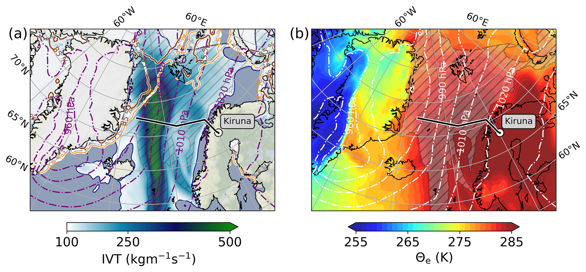
Figure 1 Synoptic ERA5-based overview of the AR event on 15 March 2022, 11:00 UTC, when HALO departed from Kiruna and crossed the AR for the first time (black-white bold line). Grey hatches show the AR boundaries according to the AR catalogue of Lauer et al. (2023). (a) shows contours of the magnitude of IVT, and (b) shows the pseudo-equivalent potential temperature (Θ_e) at the 850 hPa level. Surface isobars are given as purple (a) and white (b) contour lines. Sea ice fractions above 0.15 and 0.85 are shown as brownish lines in (a) and greyish lines in (b). Background map made with Natural Earth.

2.3 Arctic atmospheric river event

The meteorological conditions during the first week of HALO-(𝒜𝒞)³ (middle of March 2022) were characterised by a sequence of warm and moist air intrusions, some of which met the criteria for ARs in terms of the intensity of moisture transport and geometric extent. Walbröl et al. (2024) showed that these ARs were notably strong in terms of IVT for common Arctic ARs and entered the Arctic via typical paths along the North Atlantic, steering towards the Fram Strait and Barents Sea before partially reaching the Arctic Ocean.

In this case study, we focus on the strongest AR event of HALO-(𝒜𝒞)³, which entered our region of interest (Greenland Sea and Fram Strait) on 15 March 2022, sampled during research flight 05 (RF05, Fig. 1). Walbröl et al. (2024) classified this AR as a very strong event for Arctic conditions. Here, we describe the synoptic conditions causing the AR and its temporal evolution towards the following day, when the AR was observed by a subsequent research flight (RF06).

2.3.1 Synoptic conditions

A preceding rapid cyclogenesis led to a “bomb” cyclone (air pressure drop greater than 24 hPa d⁻¹, as defined in Sanders and Gyakum, 1980) in southern Greenland. Between the Norwegian Sea and Greenland Sea, the intense steering low and a Scandinavian ridge of high pressure created strong zonal pressure gradients, featuring a predominantly meridional circulation (Walbröl et al., 2024). On 15 March 2022 (RF05), the cyclone exhibited a core air pressure <960 hPa off the coast of the Denmark Strait, while high air pressure above 1020 hPa prevailed over Scandinavia (Fig. 1). The meridional circulation advected moist (Fig. 1a) and warm (Fig. 1b) air masses poleward over the Greenland Sea, leading to exceptional air mass conditions in this region (Walbröl et al., 2024), with IVT up to 500${\mathrm{kg}\mathrm{m}}^{-\mathrm{1}}{\mathrm{s}}^{-\mathrm{1}}$ over large areas along the AR in a northward orientation (Fig. 1a).

The AR crossed the marginal sea ice zone and sea ice edge from the Denmark Strait towards the northern tip of Svalbard. Horizontally compressed isobars indicate strong winds driving the intense horizontal transport. This moisture transport was associated with very warm air masses according to the 850 hPa pseudo-equivalent potential temperature Θ_e (Fig. 1b), causing record warming in the Arctic. Θ_e exceeded 285 K over a large area extending from the AR along the 0° meridian to Scandinavia. The meridional flow thus caused a strong advection of warm and moist air. Over Central Greenland, the latent warming was less pronounced, with Θ_e≤270 K and a cold western coast of Greenland with Θ_e≤260 K. While the majority of the AR was located in air masses with Θ_e≥280 K), the western AR flank behind the AR propagation showed strong gradients. They indicate the presence of a cold front favouring the intrusion of moderately colder and drier air masses to the west of the AR.

2.3.2 Evolution of the atmospheric river

HALO sampled the AR on 2 consecutive days (Fig. 2), during which the AR propagated north-eastward, with its eastern flank west of Svalbard during RF05 and east of it during RF06, before approaching the Norwegian coast with its southern end. While the AR reached its maximum intensity before both RFs (Walbröl et al., 2024), HALO observed the AR during its dissipation north of 70°, within the ICON-2km model domain. During RF05 (Fig. 2a), IVT values still reached up to $\mathrm{500}{\mathrm{kg}\mathrm{m}}^{-\mathrm{1}}{\mathrm{s}}^{-\mathrm{1}}$, while IVT dropped below $\mathrm{300}{\mathrm{kgm}}^{-\mathrm{1}}{\mathrm{s}}^{-\mathrm{1}}$ during RF06 (Fig. 2b). One reason for the decay of the AR is the reduction of the horizontal pressure gradients, which decelerates the winds. The IWV from dropsonde observations (Fig. 2) shows that the atmosphere became drier within the AR from RF05 to RF06. South of the RF06 flight path, an intensification of moisture transport was identified, which is attributed to orographic convergence. Based on the ERA5 AR catalogue of Lauer et al. (2023), the dissipation of the AR resulted in the moisture transport filaments no longer being classified as AR during RF06 (Fig. 2b). Still, the moisture transport remained high enough to be classified as AR for Arctic conditions but in a too-narrow and disturbed flow.

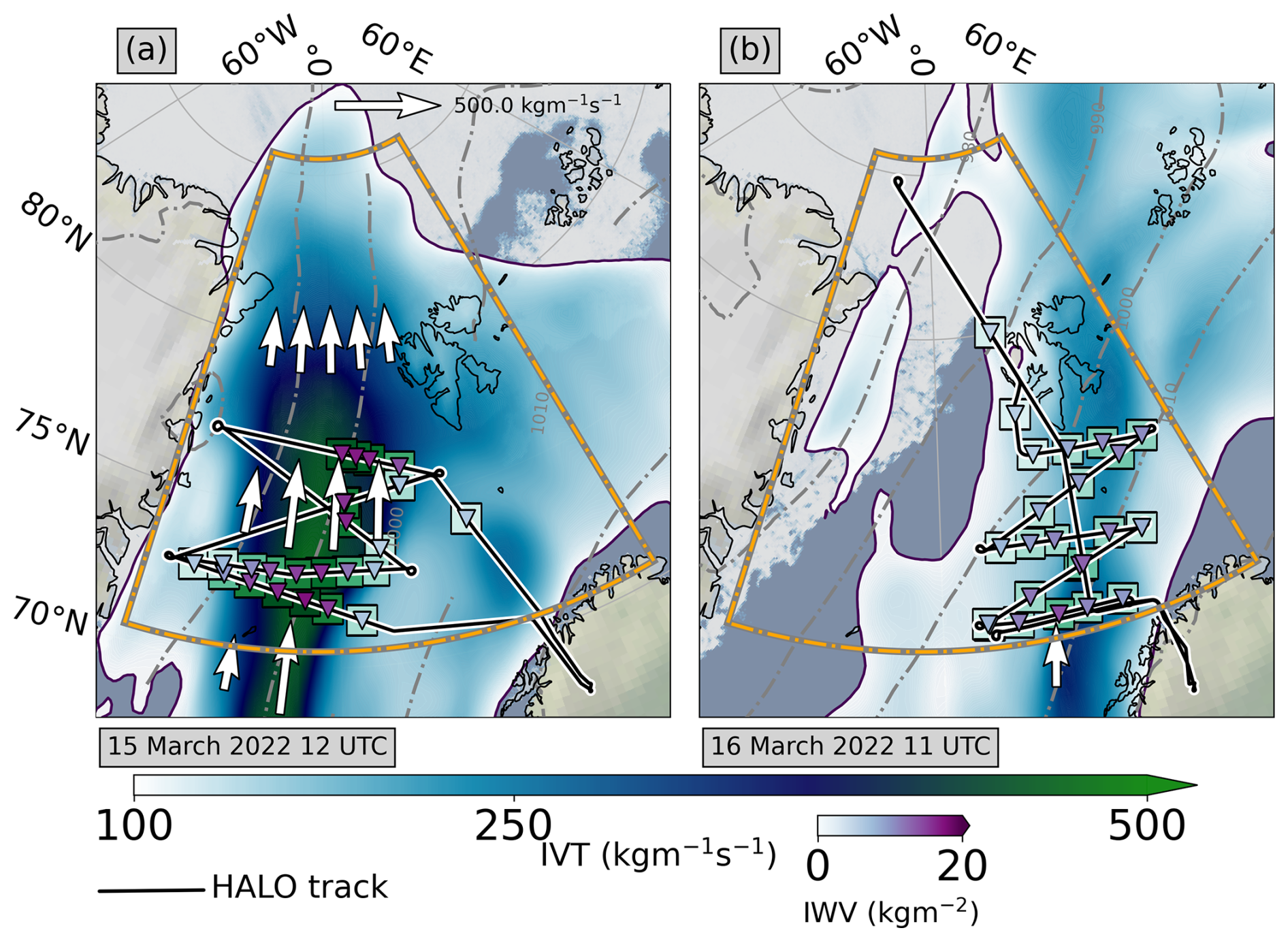
Figure 2 ERA5-IVT contours for (a) 15 and (b) 16 March 2022 of the AR, consecutively sampled by HALO. Coloured squares (triangles) indicate dropsonde values of IVT and IWV. Grey contour lines depict the surface pressure isobars. Sea ice maps are based on the AMSR-2 sea ice product provided by the University of Bremen (Spreen et al., 2008). The orange quadrangle represents the ICON-2km model domain. Background map made with Natural Earth.

RF05 and RF06 sampled different air masses of the AR. While RF05 captured the AR between its centre and the exit region, RF06 was located in the entrance region. The matching of the same air masses on consecutive days, one of the HALO-(𝒜𝒞)³ objectives (Wendisch et al., 2024), could not be achieved for both flights due to air traffic control (ATC) restrictions.

3 Estimation of moisture budget components using airborne observations

The atmospheric moisture budget is the major framework of this study to investigate the transformation of moisture in the Arctic AR. From a vertically integrated perspective, the moisture budget components are defined as:

$$\begin{array}{}\text{(1)}& \begin{array}{rl}& \underset{\mathrm{Local}\mathrm{change}\mathrm{in}\mathrm{integrated}\mathrm{water}\mathrm{vapour}}{\underbrace{{\displaystyle \frac{\mathit{\delta }\mathrm{IWV}}{\mathit{\delta }t}}}}=\underset{\mathrm{Evaporation}}{\underbrace{E}}-\underset{\mathrm{Precipitation}}{\underbrace{P}}\\ & -\underset{\mathrm{Horizontal}\mathrm{divergence}\mathrm{of}\mathrm{integrated}\mathrm{water}\mathrm{vapour}\mathrm{transport}}{\underbrace{\mathbf{\nabla }\cdot \mathit{I}\mathit{V}\mathit{T}}}\\ & +\underset{\mathrm{Residual}}{\underbrace{\mathit{ϵ}}},\end{array}\end{array}$$

with all components in kilograms per metre squared per second and in millimetres per hour when divided by the density of water. Precipitation and evaporation refer to surface values, while the integrated water vapour IWV and integrated water vapour transport IVT are vertical integrals defined as:

$$\begin{array}{}\text{(2)}& \mathrm{IWV}=-{\displaystyle \frac{\mathrm{1}}{g}}\underset{p_{\mathrm{sfc}}}{\overset{p_{\mathrm{top}}}{\int }}q\mathrm{d}p,\end{array}$$

$$\begin{array}{}\text{(3)}& \mathit{I}\mathit{V}\mathit{T}=-{\displaystyle \frac{\mathrm{1}}{g}}\underset{p_{\mathrm{sfc}}}{\overset{p_{\mathrm{top}}}{\int }}q\mathit{V}\mathrm{d}p,\end{array}$$

with the gravitational acceleration g. The specific humidity q and horizontal wind vector V are vertically integrated over the pressure (p) from the surface (p_sfc) to the top of the troposphere (p_top). When we provide IVT values, we refer to its magnitude.

Equation (1) is not necessarily closed from observations (the left-hand side is not equal to the physical processes on the right-hand side), as each component is derived independently. A residual ϵ may need to be added to achieve equality. Furthermore, ϵ can include secondary processes, such as the moisture flux through a tilted pressure surface, as described by Seager and Henderson (2013), which, however, is overall minor in ARs (Guan et al., 2020). Another process is the contribution of cloud condensate, but it is up to 2 orders of magnitude smaller than water vapour. The divergence of moisture transport affects the moisture budget in two ways, which we can attribute by splitting ∇ ⋅ IVT into:

$$\begin{array}{}\text{(4)}& \begin{array}{rl}& \mathrm{\nabla }\cdot \text{IVT}=-{\displaystyle \frac{\mathrm{1}}{g}}\underset{p_{\mathrm{sfc}}}{\overset{p_{\mathrm{top}}}{\int }}\mathbf{\nabla }\cdot \left(q\mathbf{\text{V}}\right)\mathrm{d}p=-{\displaystyle \frac{\mathrm{1}}{g}}\underset{p_{\mathrm{sfc}}}{\overset{p_{\mathrm{top}}}{\int }}\\ & \underset{\mathrm{Mass}\mathrm{divergence}\left({\mathrm{DIV}}_{\mathrm{mass}}\right)}{\underbrace{q\left(\mathbf{\nabla }\cdot \mathbf{\text{V}}\right)}}\mathrm{d}p+{\displaystyle \frac{\mathrm{1}}{g}}\cdot \underset{p_{\mathrm{sfc}}}{\overset{p_{\mathrm{top}}}{\int }}\\ & \underset{\text{Horizontal moisture advection}\left({\mathrm{ADV}}_q\right)}{\underbrace{\mathbf{\text{V}}\cdot \left(-\mathrm{\nabla }q\right)}}\mathrm{d}p.\end{array}\end{array}$$

The first term on the right side of Eq. (4) represents the dynamical mass divergence, which is the product of specific humidity and horizontal divergence. The mass divergence can be related to vertical velocity via the continuity equation and is closely linked to precipitation (Wong et al., 2016; Norris et al., 2020). The right side's second term of Eq. (4) represents the horizontal advection of moisture that Guan et al. (2020) show to be only slightly correlated to precipitation formation. Instead, it locally affects the amount of water vapour. We define the vertically integrated decompositions in Eq. (4) as IDIV_mass and IADV_q, respectively.

3.1 Flight patterns and categorisation of atmospheric river sectors

For the airborne derivation of all components of the moisture budget, i.e. our first research goal (G1, Sect. 1), flight patterns must sample areas of the AR in a specific way. Flight tracks that enclose areas, such as circles, are often used to calculate the mesoscale horizontal divergence (e.g. Bony and Stevens, 2019; Paulus et al., 2024). However, if a single circle as large as the lateral extent of the AR is used, the internal heterogeneity of moisture and wind fields within the AR, particularly across the embedded cold front, would be smoothed out in the divergence calculations (Cobb et al., 2021a; Dorff et al., 2024b). The high lateral variability in the moisture transport characteristics of ARs requires long flight legs across the AR. Therefore, Neiman et al. (2016) and Norris et al. (2020) focused their enclosing flight patterns more on the AR transect to capture this cross-sectional variability. However, their patterns were too small to cover the lateral variability of the budget components identified by Guan et al. (2020) from reanalyses.

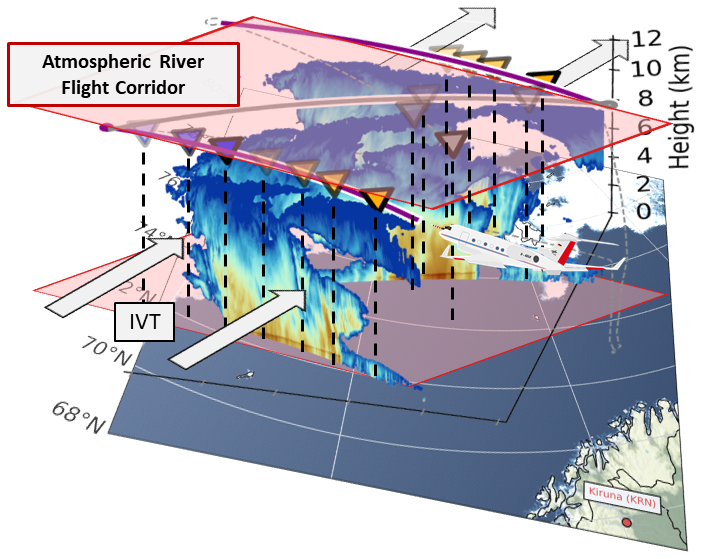
Figure 3 Realisation of a zigzag flight pattern during RF05 to derive the moisture budget components inside an Arctic AR flight corridor (the area enclosed by red rectangles). The surface map with the sea ice extent, as in Fig. 2, is superimposed with the vertical radar reflectivity curtain. Boundary flight legs (purple) quantify the ingoing and outgoing IVT via dropsondes (triangles), while the internal leg (grey) samples precipitation, evaporation, and IWV inside the AR flight corridor. Pre-frontal (post-frontal) dropsonde releases are indicated by orange (purple) triangles; internal ones are grey.

Dorff et al. (2024b) recommend full cross-sections of the AR. An internal flight leg shall connect two parallel cross-sections, resulting in a zigzag flight pattern. Figure 3 shows the realisation of the zigzag pattern for an AR flight corridor during RF05. The zigzag pattern samples the AR transverse to the IVT direction. The boundary cross-section legs perpendicular to the main flow (Fig. 3) quantify the inflow and outflow of the flight corridor, i.e. ingoing and outgoing IVT across the lateral AR extension. Dropsondes densely sample both cross-sections to derive ∇ ⋅ IVT. The internal legs explore the precipitation rate, evaporation, and water load within the AR flight corridor. The radar reflectivities in Fig. 3 show very deep clouds in the AR for Arctic conditions. The cloud top height is up to 12 km. Significant radar echoes down to the surface were recorded in the AR core (middle of the cross-sections). The high reflectivity band at about 1–2 km high (Fig. 3), a so-called bright band, indicates a melting layer. Bright bands result from snowflakes coated by liquid water, causing higher radar reflectivities (Gray et al., 2001). Below, liquid precipitation can be expected.

We divide sectors along the lateral AR cross-sections in Fig. 3, similar to the approach suggested by Guan et al. (2020). This distinction considers the presence of a cold front embedded in ARs (Ralph et al., 2004), whereby different thermodynamic conditions prevail on both sides of the front. Guan et al. (2020) calculate the moisture budget across the main AR axis and the embedded front and report on significant differences in the budget components across the AR (front). For our AR, the gradients of Θ_e (Fig. 1b) suggest remnants of a cold front. We thus divide the AR flight corridors into eastern and western parts. Concerning the approximate location of the cold front, we refer to the eastern (western) half as the pre-frontal (post-frontal) sector. This two-sector separation is shown in Fig. 3 by the orange sondes referring to the pre-frontal sector.

Recent studies (Guan et al., 2020; Cobb et al., 2021a; Dorff et al., 2024b) categorise ARs into three sectors, with the AR core as a separate one between the pre- and post-frontal sectors, containing IVT values ≥80 % of the maximum IVT. However, given the nature of the irregular sonde spacing and the purpose of including as many sondes as possible in the sector-based divergence calculations, we assign the sondes released in the eastern part of the AR core to our pre-frontal sector and those in the western part to the post-frontal sector. We restrict the extent of our sector to the actual positions of the outer sonde releases.

During RF05, ATC restrictions in Danish airspace extending over the western regions of the AR flight corridors did not allow sonde releases in the post-frontal sector for the northern cross-sections (Fig. 3). This lack of data prevents reliable sonde-based divergence estimates for post-frontal sectors. Hence, the subsequent analysis is confined to pre-frontal AR sectors. Upcoming sections refer to the pre-frontal sector defined by the connection of the orange sonde locations in Fig. 3, henceforth denoted as S1. We consider S1 to demonstrate the derivation of each moisture budget component included in Eq. (1) using HALO.

3.2 Local change in integrated water vapour ($\mathit{\delta }\mathrm{IWV}/\mathit{\delta }t$) from radiometer

The IWV is most accurately determined using dropsonde measurements of vertical moisture profiles. However, these dropsonde profiles have limited spatial coverage. The few internal profiles may thus lack spatial representativeness for estimating the local change in IWV within the pre-frontal AR sector. To address this issue, we use the quasi-continuous HAMP radiometer measurements of the channels from 22 to 190.81 GHz (Sect. 2.1). Their 1 s measured T_B values are very sensitive to the emitted radiation from water vapour across the microwave spectrum (Jacob et al., 2019). In particular, the K-band channels of HAMP show rising T_B with increasing IWV. Furthermore, continuum water vapour absorption influences the T_B at window frequencies near 30 and 90 GHz.

From the observed T_B values, the IWV can be estimated using appropriate retrieval methods. We build a linear regression model retrieval, as used in Jacob et al. (2019), which we describe in Appendix A. As specified in Sect. A1, the regression coefficients between the two quantities (IWV and T_B) are based on a training dataset containing meteorological fields from ECMWF Reanalysis v5 (ERA5), along with synthetic T_Bs generated from the forward simulator PAMTRA (Passive and Active Microwave TRAnsfer tool; Mech et al., 2020). Applying the emerging retrieval coefficients to the measured T_B, the retrieved IWV data show a good agreement with the dropsonde-based IWV over a wide range from 6 to 18 kg m⁻². Furthermore, the comparison of the airborne-retrieved IWV values with the collocated and continuous ERA5-based representation confirms that the continuous HAMP representation reasonably replicates the IWV values (Sect. A2; Fig. A1).

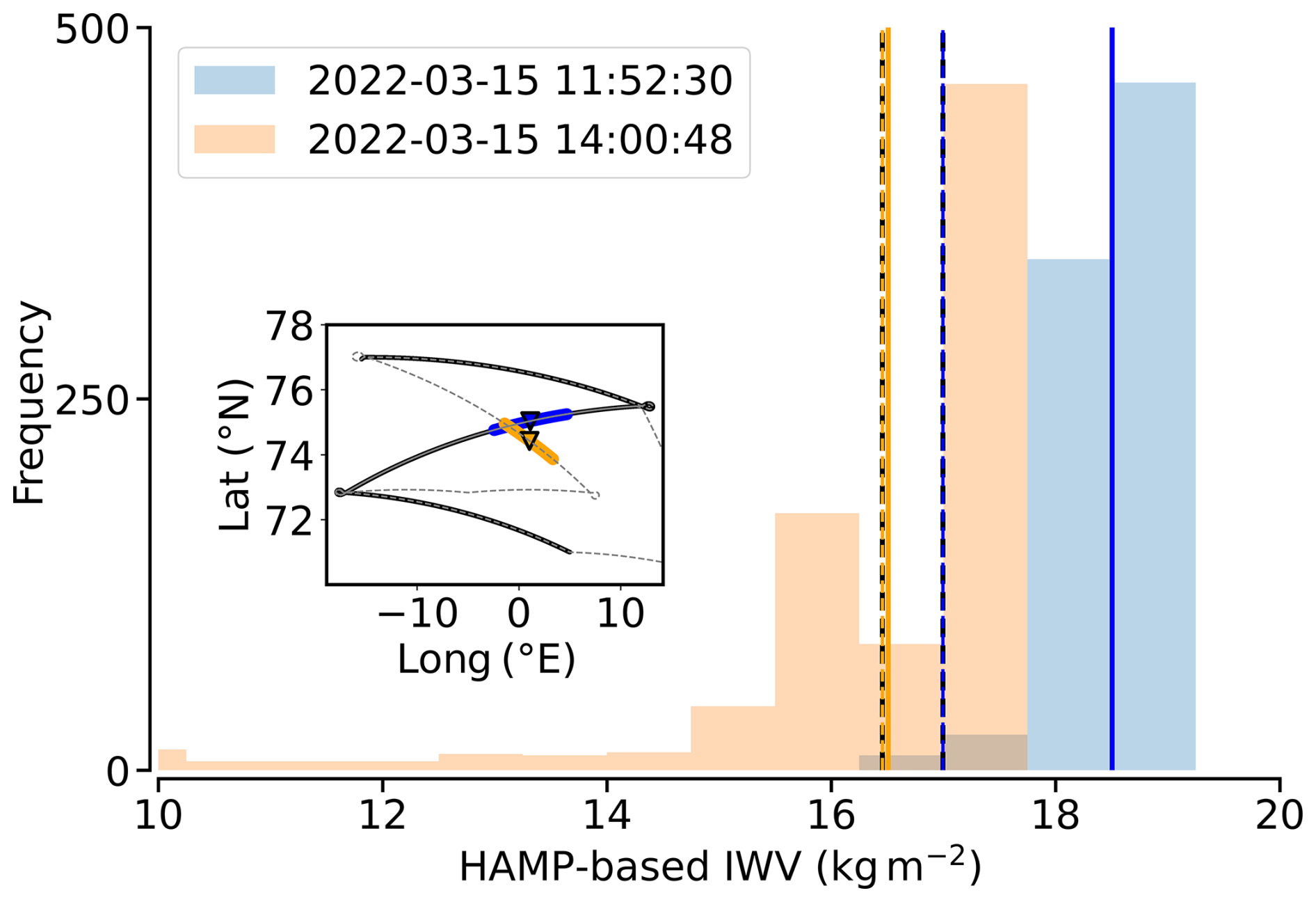
Figure 4 Determination of local change in IWV from the first sector S1 in the AR during RF05. The sub-panel demonstrates the internal flight leg segments used for estimating the change in IWV internal of S1 and two dropsonde releases (triangles) inside. Flight leg segments extend symmetrically around the sondes, whose release times are specified in the legend. For both legs, their HAMP-based IWV distribution is illustrated with their respective mean values (bold solid lines). The dashed vertical lines specify sonde-based values.

To derive the local temporal changes in HAMP-retrieved IWV within the AR flight corridors, we consider the internal flight legs of the zigzag pattern (Fig. 3). The derivation of $\mathit{\delta }\mathrm{IWV}/\mathit{\delta }t$ requires sampling a specific region at two distinct time steps. This requirement is met within the AR core at the crossing flight paths. However, the single intersection in Fig. 4 has limited representativeness for the entire sector, and the internal flight legs separate from each other in the pre-frontal sectors. Therefore, we opt to compare only segments of internal flight legs (of about 100 km) that lie close to each other, without considering single locations (Fig. 4). Symmetrically around two sonde releases, we assess the “local” change in IWV over approximately 2 h.

While the dropsonde-based IWV values in Fig. 4 differ by less than 1 kg m⁻², the HAMP-based mean values of each leg differ by more than 2 kg m⁻². The IWV distributions along the leg segments (Fig. 4) reveal a high spatial variability because we consider regions of strong IWV gradients. This variability leads to significant uncertainties in estimating local changes in IWV. To quantify these uncertainties, we subsequently extend the internal leg segments by a minute (starting from 1 and going up to 10 min) and calculate the standard deviation of the mean local IWV change across all segments. For the pre-frontal AR sector S1, we thus derive a value of local change in IWV of $\mathrm{-}\mathrm{0.79}\pm \mathrm{0.19}{\mathrm{mm}\mathrm{h}}^{-\mathrm{1}}$. Because the resulting uncertainties are much larger than those based on the regression retrieval, we neglect retrieval uncertainties in the uncertainty assessment of $\mathit{\delta }\mathrm{IWV}/\mathit{\delta }t$.

3.3 Evaporation (E) estimated from dropsonde data

The surface evaporation E can be estimated from bulk approaches, taking into account surface wind, temperature, and humidity. Our calculations are based on the aerodynamic bulk methods of Rao et al. (1981), who derive the surface evaporation as:

$$\begin{array}{}\text{(5)}& E=c_{\mathrm{d}}{\mathit{\rho }}_{\mathrm{a}}(q_{\mathrm{s}}-q_{\mathrm{a}})\cdot V,\end{array}$$

where q_a is the near-surface specific humidity and q_s is the saturation specific humidity for the current sea surface temperature (SST). ρ_a represents the air density near the sea surface. c_d is the evaporation drag coefficient, where we follow Howland and Sikdar (1983) and separate c_d for two wind regimes, with $c_{\mathrm{d}}=\mathrm{1.4}\times {\mathrm{10}}^{\mathrm{3}}$ for winds $\le \mathrm{14}{\mathrm{m}\mathrm{s}}^{-\mathrm{1}}$ and $c_{\mathrm{d}}=\mathrm{1.6}\times {\mathrm{10}}^{\mathrm{3}}$ for higher wind speeds V. We obtain the near-surface values from the lowest dropsonde profile levels before reaching the sea surface (below 50 m). We filter out values from heights below 0 m, as the sondes sometimes transmit data just after they enter the sea. In other cases, erroneous GPS altitude data may prevent near-surface classification, so the corresponding sondes are omitted. We calculate q_s for the SST extracted from the collocated ERA5 data. The air density is based on the near-surface sonde pressure, humidity, and temperature values. Uncertainties in the derived evaporation result from Gaussian error propagation of the sonde-based quantities given in Bony and Stevens (2019).

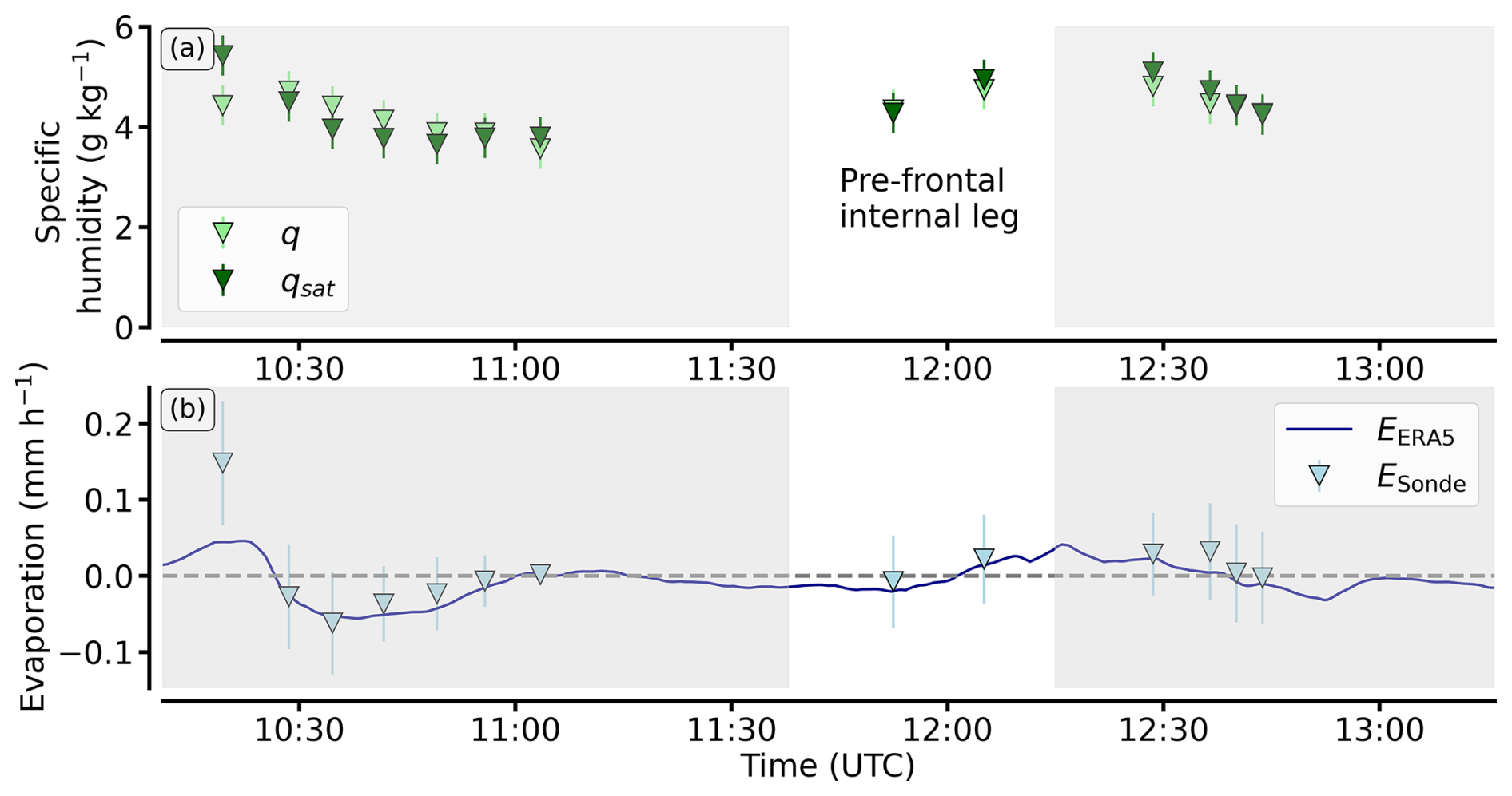
Figure 5 Dropsonde-based evaporation derivation for the first AR flight corridor of RF05. The sonde-based near-surface specific humidity and the saturation specific humidity for the given SST extracted from ERA5 are presented (a). Triangles in (b) represent the sonde-based ocean evaporation resulting from the values in (a). The pre-frontal segment of the internal leg relevant to S1 is highlighted (white). The continuous blue line depicts collocated ERA5-based evaporation.

Looking at the first complete zigzag pattern that contains S1, Fig. 5a shows that sonde-based deviations between q_s and q_a are quite small, except for the first sonde. This indicates near-saturated air, with some sondes even showing super-saturated air. Sondes in supersaturation reveal small negative values in evaporation (condensation). Overall, the evaporation is weak, with absolute values below 0.05 mm h⁻¹ most of the time (Fig. 5b). The uncertainties in q are much smaller than the actual values of q but non-negligible (Fig. 5a). Based on the two sondes within the pre-frontal internal flight segment, we calculate a mean evaporation of 0.01 ± 0.06 mm h⁻¹.

Comparison with collocated ERA5 (Fig. 5b) verifies that the sonde-based bulk values of E are in a realistic order of magnitude. ERA5 confirms the very small contribution of evaporation to the moisture budget within the AR flight corridor. Note that Fairall et al. (2003) suggest more detailed calculations of evaporation. However, given the overall agreement of our sonde-based results with model data (Fig. 5), the simplified approach in Eq. (5) appears to be appropriate for Arctic ARs with small E.

3.4 Precipitation based on radar

We obtain the precipitation rates by using the cloud and precipitation radar measurements from the unified dataset (Sect. 2.1; Dorff et al., 2024a). These radar reflectivities are offset-calibrated following Ewald et al. (2019). In addition, we correct the reflectivities for gaseous attenuation by water vapour, which we calculate from the model of Rosenkranz (1998) using water vapour profiles from the ECMWF Integrated Forecast System (IFS) model. The conversion of radar reflectivity into precipitation rates is conventionally achieved by the application of empirically derived radar reflectivity to rain rate (Z-R) relationships (e.g. Marshall and Palmer, 1948). The Z-R relationships are provided by power laws in the form of Z=aR^b; see Table 1. The parameters a and b account for variations in precipitation for a given reflectivity, arising from differences in the particle size distribution (PSD). However, the parameters vary greatly between radar frequencies, measurement viewing angles, and precipitation types (Ignaccolo and De Michele, 2020). Using shipborne disdrometer data, Neiman et al. (2017) mentioned the rapid spatiotemporal evolution of drop size distributions as an AR-specific caveat to using a single Z-R relationship.

This dilemma is exacerbated in Arctic ARs, where the coexistence of different precipitation phases (liquid and solid) is expected. The radar bright band shown in Fig. 3 provides evidence that melting of precipitation occurs in our AR event such that we observe rainfall and snowfall. The airborne estimation of precipitation rates along the internal legs for our moisture budget closure is thus 2-fold, based on Austen (2023). This estimation requires a precipitation type classification using a melting layer detection, followed by the application of a set of multiple Z-R and reflectivity-to-snow (Z-S) relationships (Table 1).

For the precipitation type classification, we use the linear depolarisation ratio (LDR) included in Dorff et al. (2024a). In the first internal flight leg, high reflectivity bands frequently occur (Fig. 6a), while the LDR represents a robust indicator for the melting layer (Fig. 6b). For the melting layer detection, Illingworth and Thompson (2011) propose an LDR threshold of −17 dB, which we apply to our radar data. The nearest-surface exceedance of the threshold marks the bright-band bottom BB_bottom.

Marshall and Palmer (1948)Norris et al. (2020)Chandra et al. (2015)Schoger et al. (2021)Matrosov (2007)Heymsfield et al. (2018)

Table 1 Overview of used Z-R and Z-S relationships, categorised by the radar bands applied, how they were derived, and their representativeness.

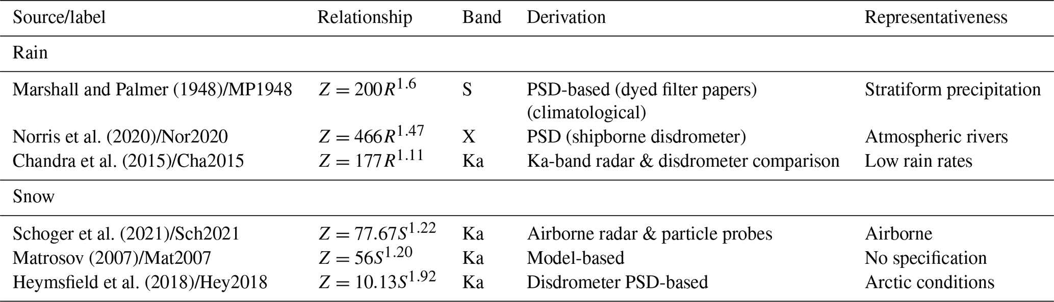
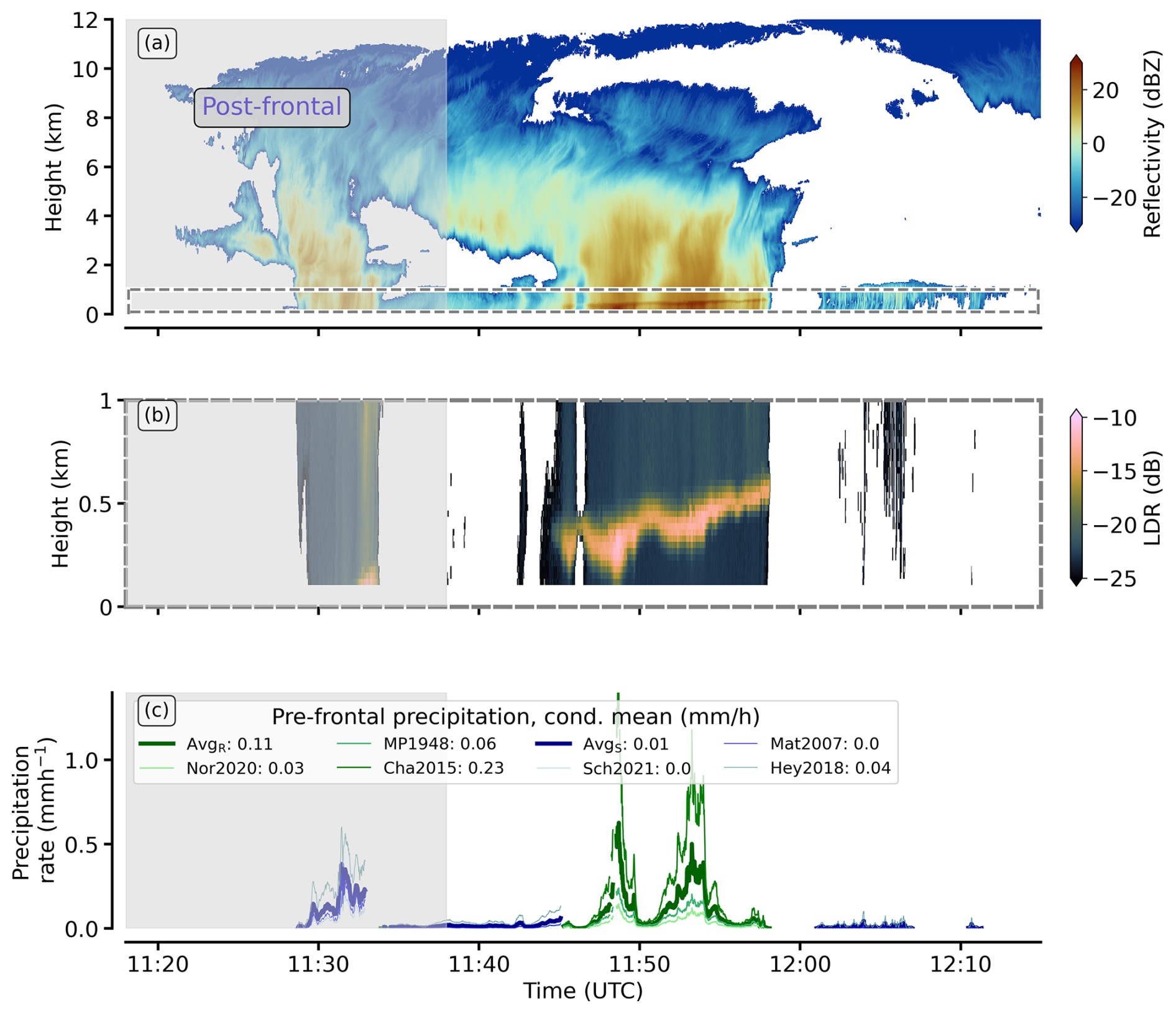
Figure 6 Radar reflectivity (a), LDR (b), and derived precipitation rate (c) for the internal leg in the first AR corridor. The post-frontal segment is sketched in grey. The dashed rectangle in (a) specifies the zoomed-in area of the plotted LDR in (b). Green (blue) precipitation rates in (c) refer to rain (snow) rates classified by the melting layer algorithm. The legend entries in (c) refer to the labels of the relationships defined in Table 1 and specify mean conditional precipitation rates for the pre-frontal segment of the internal flight leg and the respective relationship. Average values over all corresponding relationships are shown as bold lines for rain (Avg_R) and snow (Avg_S), respectively.

However, such a pure threshold-based melting layer detection is subject to many artefacts and outliers. Therefore, we apply additional criteria. First, the maximum BB_bottom height is set to 2000 m, and then its spatial gradient is restricted. We consider variations of BB_bottom of up to 60 m per 200 m horizontal distance as realistic. Both vertical thresholds are checked for a rolling mean window of 5 s, which is applied to the initially pure LDR-based BB_bottom. While the gradient threshold is very suitable for most RF legs, it is too restrictive near front regions such as those that occur across ARs, where air mass transitions can cause vertical changes in the melting layer of several hundred metres in 1 km (e.g. Fig. 6b; 11:48). For this reason, we add gap-filling by linear interpolation, allowing for maximum gap lengths of ≈2.5 km. These gap-filled periods are the ordinary BB_bottom. We declare precipitation below the presence of BB_bottom as rain and, if no bright band is found, as snowfall.

We account for a transition zone where mixed-phase precipitation is likely, as phase transitions do not occur immediately. We define periods of possible mixed-phase precipitation type by an additional interpolation over the remaining data gaps of BB_bottom up to ≈2 km and by extrapolation of BB_bottom of ≈2 km along the flight. Furthermore, mixed-phase precipitation becomes ubiquitous as the bright band descends to the surface. The near-surface BB reflectivities can then lead to an overestimation of precipitation rates. To prevent this, all corresponding precipitation periods with BB_bottom<300 m are treated as uncertain.

The precipitation phase classification allows the derivation of precipitation rates to distinguish between snow and rain periods. This is essential because the Z-R and Z-S relationships are quite different due to the different scattering properties of the hydrometeors. We consider six reflectivity-rate relationships (Table 1). Each of these relationships considers different aspects relevant for our Ka-band radar estimates of precipitation in Arctic ARs. In particular, the relationships weigh lower and higher reflectivity factor values differently. None of the relationships listed are optimal for our purposes. However, the variety of their different representativeness gives us a higher chance of reproducing the high PSD variability in AR conditions as found by Norris et al. (2020). Therefore, we apply all relationships to our precipitation-phase-classified reflectivities and consider their spread to estimate our uncertainties.

We find different precipitation modes for the first internal leg (Fig. 6). While the western post-frontal sector shows convective cells, there is very deep convection in the AR core and its eastern part belonging to S1, which contains two major precipitation fields (Fig. 6c). Further east in the pre-frontal sector (Fig. 6; right side), precipitation becomes weaker and more stratiform. While the cell in the post-frontal (cold) sector is snow, the melting layer in the heavy precipitation core rises towards the warm pre-frontal sector (Fig. 6b, c). Within the pre-frontal half of the core, precipitation contains rain with mean rates greater than 0.5 mm h⁻¹, while the rates based on the relationship of Chandra et al. (2015) exceed 1 mm h⁻¹. In particular, for more intense precipitation, the rates between the relationships increasingly diverge (Fig. 6c), leading to higher uncertainties in the precipitation estimate for the moisture budget closure. For the pre-frontal segment of the internal leg, we derive a mean precipitation rate of 0.05 mm h⁻¹, with an uncertainty range from 0.01 to 0.11 mm h⁻¹.

The Arctic precipitation rates we derive are much lower than the airborne precipitation rates in mid-latitude ARs by Norris et al. (2020). Yet, our approach may underestimate precipitation because we neglect hydrometeor attenuation, which becomes relevant for estimates near the surface when the radar signal has to penetrate deep rain clouds with melting layers. Obtaining estimates of the magnitude of melting layer attenuation is complex. Approaches such as the path-integrated attenuation correction by Meneghini et al. (2015) are not feasible for our radar, as the receivers' high pulse power and high sensitivity lead to overdriven ground return.

3.5 Moisture transport divergence (∇IVT) based on dropsondes

For the dropsonde-based determination of the IVT divergence, we follow the methods of Bony and Stevens (2019) and Dorff et al. (2024b). We derive both composites of the moisture transport divergence, namely, mass divergence (DIV_mass) and moisture advection (ADV_q) in Eq. (4), using a regression approach applied to the respective sonde-based wind and moisture fields. In the case of linear variations, a time-stationary meteorological quantity Φ (e.g. wind speed) can be inferred as:

$$\begin{array}{}\text{(6)}& \mathrm{\Phi }={\mathrm{\Phi }}_{\mathrm{o}}+{\displaystyle \frac{\mathit{\delta }\mathrm{\Phi }}{\mathit{\delta }x}}\cdot \mathrm{\Delta }x+{\displaystyle \frac{\mathit{\delta }\mathrm{\Phi }}{\mathit{\delta }y}}\cdot \mathrm{\Delta }y,\end{array}$$

where Φ_o is the area mean and Δx and Δy are zonal and meridional displacements from the area centre point. Using the values of Φ at sounding locations and minimising the least-squares errors in the linear regression fit of Eq. (6), linear estimates of the zonal (x) and meridional (y) gradients are obtained. We calculate the divergence by summing the two gradients. The uncertainty in derived divergence is estimated by Gaussian error propagation from the uncertainty of the fitted regression coefficients.

We determine both the divergence of the wind vector field and the gradients of the moisture field to calculate the two components DIV_mass and ADV_q and finally, as the sum of the vertical integral of both composites, ∇ ⋅ IVT (Eq. 4). Uncertainties of ∇ ⋅ IVT are non-trivial due to possible statistical dependence of the values along the vertical profile. While Norris et al. (2020) used a Monte Carlo approach to circumvent this limitation, we estimate the vertical decorrelation length by referring to a common low-level jet (LLJ) vertical extent of 400 m. We average the uncertainties for DIV_mass and ADV_q in vertical 400 m bins, with the bin size as our decorrelation length estimate. We assume that these values are statistically independent, so we can apply the Gaussian and central limit theorem. The uncertainty of the vertically integrated composites, IDIV_mass and IADV_q, is calculated from the standard deviation of the respective uncertainty values in the 400 m bins, multiplied by the vertical pressure range and the number of pressure levels.

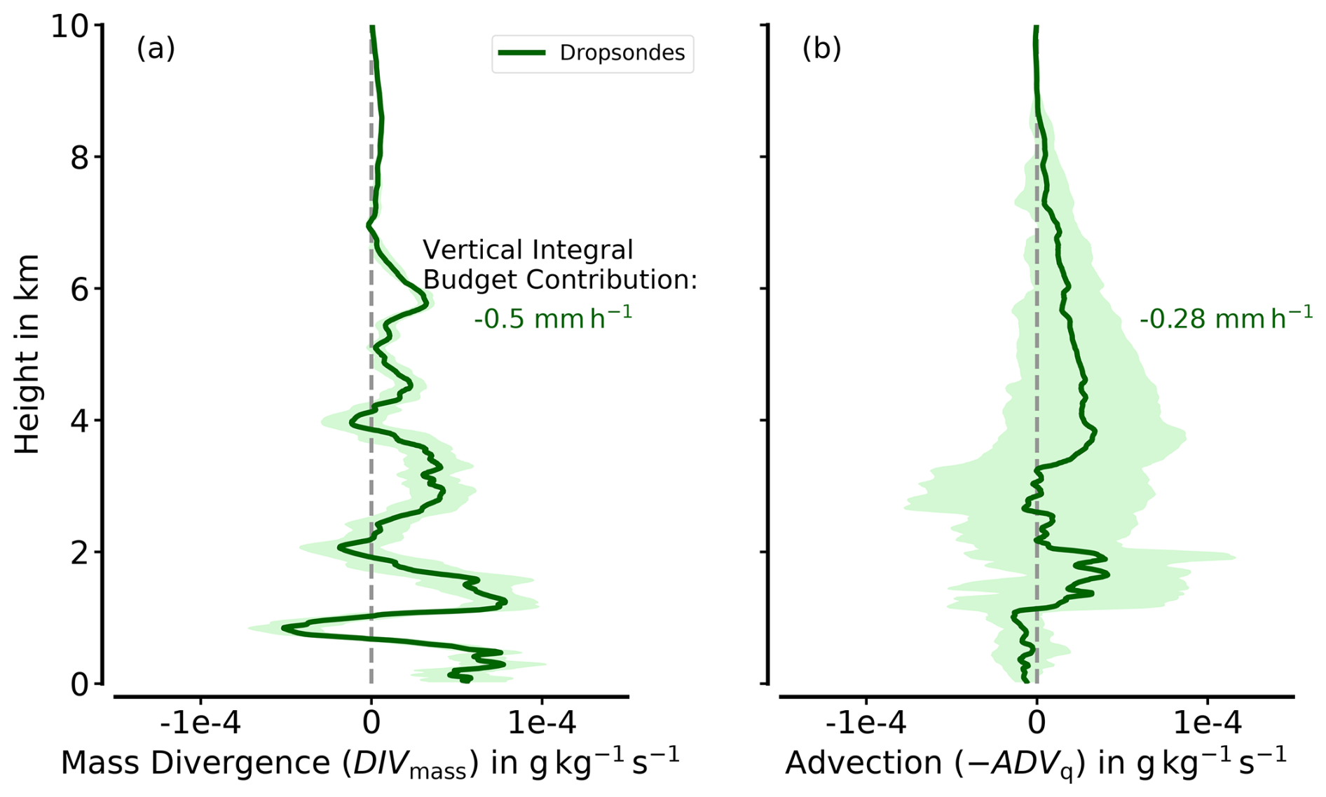
Figure 7 Sonde-based vertical profiles of mass divergence (a) and advection (b) for AR sector S1. Bold lines indicate the values based on the regression fits, while shaded areas mark the uncertainties resulting from the standard deviation in the regression fit components.

For S1, Fig. 7 shows the vertical profiles of DIV_mass and ADV_q, as derived from the sonde-based regression. For both composites, the values remain in the range of $\pm \mathrm{1}\times {\mathrm{10}}^{-\mathrm{4}}{\text{g\hspace{0.17em}kg}}^{-\mathrm{1}}{\mathrm{s}}^{-\mathrm{1}}$ and are rather low for Arctic AR conditions (Dorff et al., 2024b). Both composites contribute to the moisture budget through drying. Calculating the vertical integrals IDIV_mass and IADV_q, mass divergence causes a drying of 0.50 ± 0.06 mm h⁻¹ and dry advection of 0.28 ± 0.14 mm h⁻¹, respectively.

Both composites act differently at vertical levels. Mass divergence is most pronounced in the lower levels up to 4 km. Remarkably, the divergence is interrupted by a slight convergence at around 1 km (Fig. 7a). This is at the height of the LLJ (Ralph et al., 2005), where the sondes measure wind speeds above 30 m s⁻¹. Mass convergence near the LLJ is typical for ARs (Guan et al., 2020) and has also been identified in the Arctic ARs (Dorff et al., 2024b). At this height, mass convergence is associated with supergeostrophic winds, which enhance the moisture transport (Demirdjian et al., 2020). Except for the LLJ, divergent winds dominate the mass divergence (Fig. 7a). While wind speeds remain similar along the mid-troposphere (≈25 m s⁻¹ up to 6 km), horizontal wind divergence increases with height, mainly due to changes in wind direction. Still, the magnitude of moisture mass divergence (DIV_mass) decreases due to the superimposition of vertically decreasing moisture.

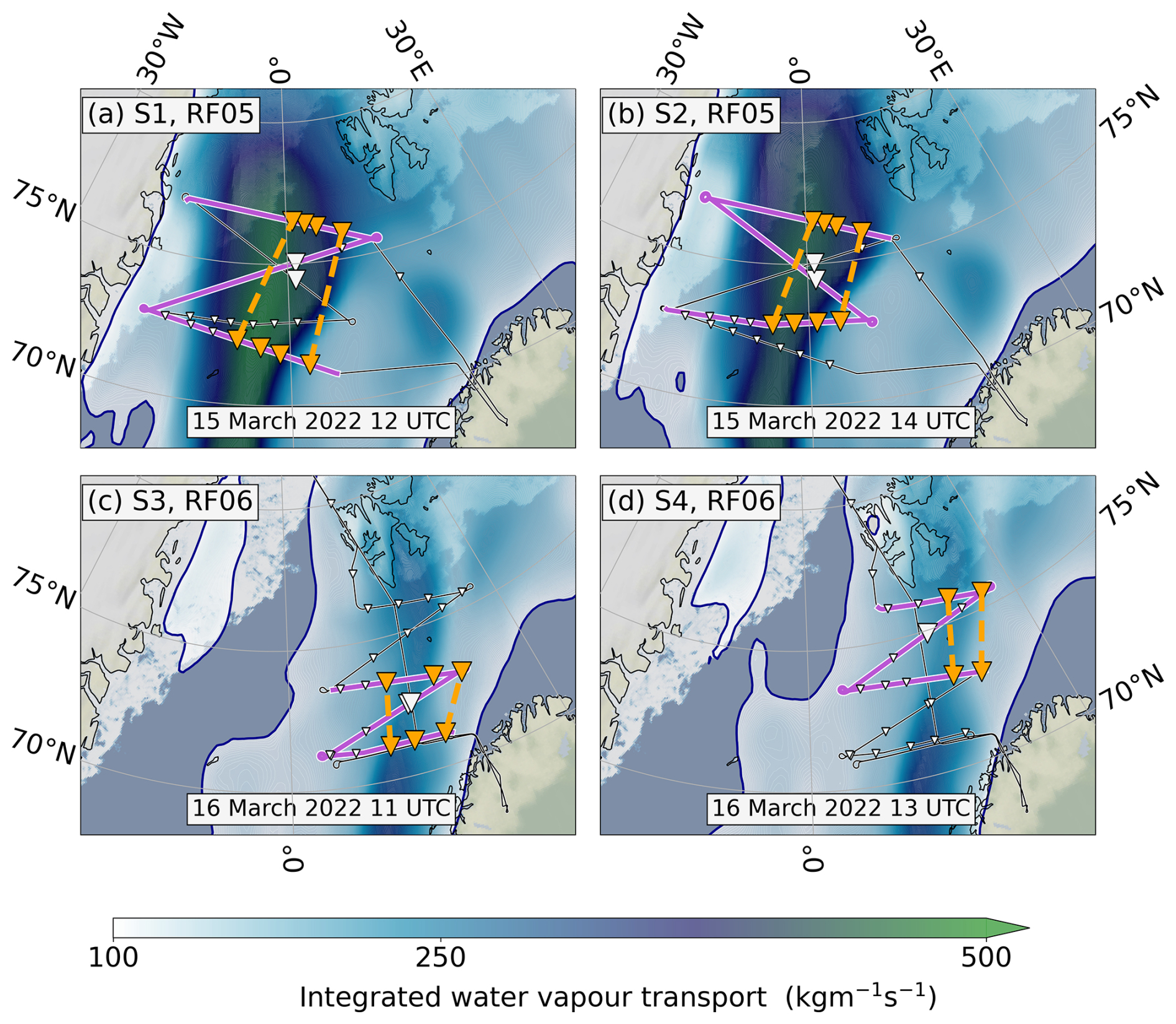
Figure 8 All four AR flight corridors sampled by the zigzag flight pattern (purple lines) in RF05 and RF06 (black/white lines). ERA5-IVT contours superimpose the sea ice map from AMSR2. Dropsondes are depicted by triangles, where orange triangles indicate the sondes spanning the pre-frontal sectors, S1–S4 (dashed orange lines). White triangles depict the sondes around which internal HAMP-based $\frac{\mathit{\delta }\mathrm{IWV}}{\mathit{\delta }t}$ was calculated. ERA5 time steps (bottom) refer to the centred hour of each zigzag pattern. Background map made with Natural Earth.

Moisture advection is low from the saturated boundary layer up to the LLJ (Fig. 7b). At these levels, all sondes indicate a very moist troposphere, with q around 4.5 g kg⁻¹. While moisture in Arctic ARs can occasionally also exceed 5 g kg⁻¹ in early summer (Viceto et al., 2022), such q values are exceptional for early spring conditions (Dorff et al., 2024b). Above the LLJ, dry advection is relevant from 1 to 2 km and above 4 km. Because the horizontal moisture gradients persist with height more than mean absolute moisture, advection decreases less with height than mass divergence. The sondes in the inflow legs partly show very dry mid-level conditions (not shown). The uncertainties increase significantly and are much higher than for mass divergence.

4 Temporal evolution of airborne AR moisture budget components

4.1 Series of pre-frontal AR sectors

To assess the temporal evolution of the AR moisture budget components (research goal G2, Sect. 1), we analyse a series of four AR flight corridors encompassed by the two flights RF05 and RF06. Figure 8 illustrates how the two zigzag patterns per RF sample the AR to derive its budget components over a period exceeding 24 h. During both RFs, the outflow leg of the first zigzag pattern simultaneously serves as a leg in the zigzag pattern for the consecutive AR flight corridor (outflow in S2, inflow in S4). Aiming to derive the full moisture budget during the AR evolution from airborne observations, our analysis focuses on the pre-frontal AR sectors (Fig. 8; orange areas) due to the ATC restrictions on western sonde releases during RF05.

The relevant sondes in the zigzag patterns cover four pre-frontal sectors (S1–S4, Fig. 8). During RF05, the sectors S1 and S2 are located in the AR exit region, over the ice-free ocean southwest of Svalbard, while in RF06, they are located south of Svalbard. The outflow leg of the last AR sector (S4) approaches the southern coast of Svalbard, crossing the marginal sea ice zone. The number of sondes used to determine ∇ ⋅ IVT in each pre-frontal sector differs in S1 and S2 compared to S3 and S4 during RF06 (Fig. 8). Eight sondes per sector are included in the divergence calculations for S1 and S2 (RF05). In turn, the pre-frontal flight legs in RF06 are shorter, resulting in only four to six sondes spanning the pre-frontal sectors. We account for the impact of the number of sondes on the accuracy of ∇ ⋅ IVT by quantifying the uncertainty in the regression coefficients.

4.2 Decay of the atmospheric river

The reanalysis IVT fields in Fig. 8 reveal a significant decay of the AR. The extended AR core, which maintained IVT ≥ 400 kg m⁻¹ s⁻¹ during RF05 (Fig. 8a, b), substantially decreased to below 300${\mathrm{kg}\mathrm{m}}^{-\mathrm{1}}{\mathrm{s}}^{-\mathrm{1}}$ (Fig. 8c, d) by the next day. For the airborne perspective, Fig. 9 illustrates the sonde-based distributions of IWV and IVT derived along each flight corridor corresponding to one of the AR pre-frontal sectors S1–S4 (Fig. 8). Comparing the sonde-based integrated quantities of the 2 flight days, the IVT values decrease by approximately 50 %, while IWV decreases by 40 %, indicating a stronger decay in the moisture transport than in the moisture fields. The box heights in Fig. 9 show that the spatial variability along the AR flight corridors decreases from those including S1 and S2 to those of S3 and S4. Similar to the median values, the decrease in variability is more pronounced for IVT than for IWV. Reducing moisture transport (IVT) is primarily driven by decreasing wind speeds with a decay of the LLJ due to decreasing pressure gradients (not shown). Note that the sonde-based decay of IWV is similarly reproduced by the continuous along-track representation of the HAMP-based IWV retrieval (not shown).

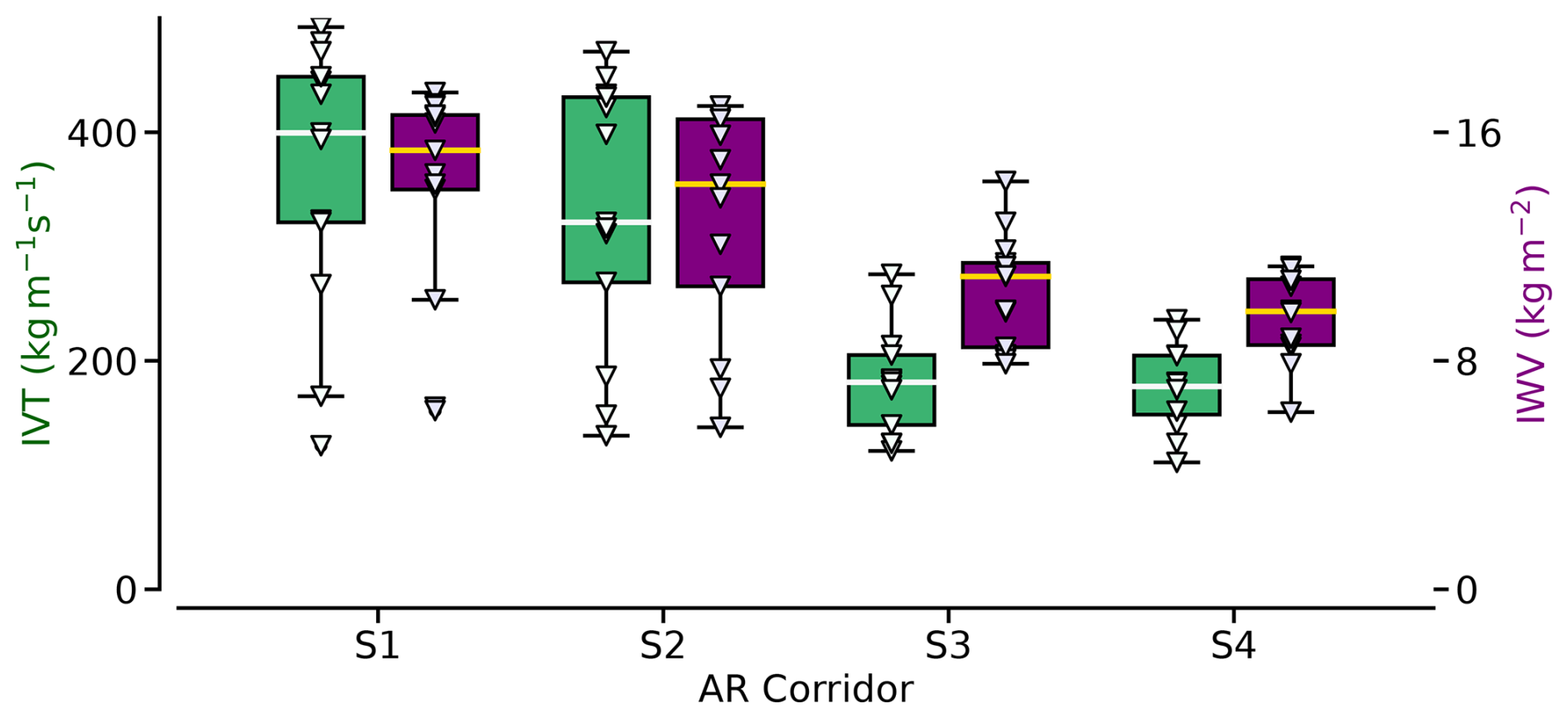
Figure 9 Box plots showing the statistics of sonde-based IVT (green) and IWV (purple) values within the four AR flight corridors, which are sampled from 2 consecutive days (S1, S2 belong to research flight RF05, while S3, S4 to RF06). The boxes show the quartiles of the datasets. The statistics refer to all sondes released inside the zigzag flight corridor, not only the pre-frontal sectors. Triangles depict the individual values of each sonde.

The distributions in Fig. 9 between two flight corridors on the same day are almost similar. Nonetheless, the medians still suggest a decaying trend of the AR on these shorter timescales. With this consistent decay of the AR, it is worth investigating how this trend can be linked to the evolution of the moisture budget components.

4.3 Comparing the moisture budget components

We compare all airborne moisture budget components, derived as described in Sect. 3, over the series of pre-frontal AR sectors and determine to what extent each component contributes to the vertically integrated moisture budget (Eq. 1). For all budget components and pre-frontal sectors, Fig. 10 shows that the individual components contribute to the moisture budget in a range of $\pm \mathrm{1}{\mathrm{mm}\mathrm{h}}^{-\mathrm{1}}$. The magnitude of these ranges is slightly lower than the reanalysis-based statistics of mid-latitude AR events in Guan et al. (2020) and nearly half the size of the airborne components derived in the mid-latitude case study conducted by Norris et al. (2020). However, our AR flight corridors and pre-frontal sectors are substantially larger than those in Norris et al. (2020). For Arctic conditions, the absolute magnitudes of IDIV_mass and IADV_q, which we derive in our AR, are comparable to distributions found in pre-frontal AR sectors in Dorff et al. (2024b).

Figure 10 shows that the AR experiences rather weak surface interaction, characterised by small mean contributions from evaporation (E) and precipitation (P). Specifically, evaporation remains notably weak, with the highest value of $E=\mathrm{0.15}{\mathrm{mm}\mathrm{h}}^{-\mathrm{1}}$ at the first sonde in Fig. 5 across both RFs. Moreover, the average pre-frontal precipitation based on the internal flight leg remains below 0.1 mm h⁻¹. Despite cloud systems' compact and deep nature within the AR core, the surface precipitation is very heterogeneous. While precipitation rates up to 1 mm h⁻¹ are derived for both rain and snow phases, they occur only for short periods. Rather, isolated moderate precipitation plumes often alternate with weak or no precipitation periods. Furthermore, stronger precipitation is partly found west of the pre-frontal budget regions.

The moisture transport divergence mainly controls the local change in water vapour for all sectors. Between advection and mass divergence, we identify mainly moisture (dry) advection aligned with the local water vapour change. This is consistent with mid-latitude ARs, where advection has been identified as being more correlated with local water vapour change (Guan et al., 2020). The convergence of mass governing the vertical motion that can trigger precipitation is very weak for this AR. Even more astonishing is the strong divergence of moisture mass during RF05, which is atypical for pre-frontal AR characteristics according to Guan et al. (2020).

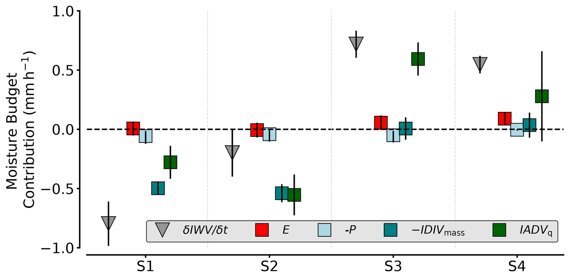
Figure 10 Hourly contribution in mm h⁻¹ of the vertically integrated moisture budget components (Eq. 1) for each of the pre-frontal sectors (S1–S4). Note that IVT convergence (−∇ ⋅ IVT) is split into both integrated summands, i.e. mass convergence (−IDIV_mass) and moisture advection (IADV_q). All components were derived from HALO. The error bars represent the uncertainties derived for each of the components.

The dominant components are those with the highest absolute uncertainties. Uncertainties in $\mathit{\delta }\mathrm{IWV}/\mathit{\delta }t$ can reach up to ± 0.25 mm h⁻¹ (e.g. S2; Fig. 10). A comparison of the two composites of ∇ ⋅ IVT shows that the uncertainties in advection are greater than those in mass divergence. This difference is due to higher spatial variability in the moisture field than in the wind field, which influences the uncertainty of the regression fits (Sect. 3.5) and thus affects the accuracy of the resulting budget components. Higher moisture variability has also been found in other Arctic ARs (Dorff et al., 2024b). In addition, the components show the dependence of the moisture transport representation on the sampling frequency (Ralph et al., 2017; Dorff et al., 2024b). The sampling of S1 and S2 involved eight sondes along both cross-sections, while only six (four) were used for S3 (S4), as shown in Fig. 8. The sectors S3 and S4 exhibit much larger uncertainties in sonde-based integrated moisture transport divergence. Particularly, the uncertainties in S4 highlight that coverage by four sondes in a frontal sector may be insufficient.

During the decaying evolution, the magnitudes of the moisture budget components remain rather constant. However, the values change in their sign. The pre-frontal AR sectors exhibit a drying of more than 0.5 mm h⁻¹ during RF05 (S1 and S2), in contrast to a surprising moistening of more than 0.5 mm h⁻¹ during RF06. Throughout this transition, the balance of local change in water vapour and moisture transport divergence and the weak precipitation and evaporation persist across all sectors. The moisture transport divergence primarily contributes to the drying of the air masses during RF05 and the moistening during RF06. Both composites of ∇ ⋅ IVT shift from divergence to convergence, while advection emerges as the predominant component over the mass divergence. Because the trends in local moisture are mainly determined by moisture transport divergence, we examine the vertical profiles of moisture advection ADV_q and mass divergence DIV_mass for all pre-frontal AR sectors in more detail. This analysis enables a specification of the evolution of the moist air masses within the AR by identifying the dominant heights of moisture transformation. We further examine how the cloud and precipitation fields respond.

4.4 Moisture transport divergence trends

Figure 11 offers insights into the evolution of moisture advection and mass divergence during the AR decay across the sectors S1–S4, illustrating the dominant terms at different heights. During S1 and S2, almost the entire profile of DIV_mass exhibits positive values, apart from the convergence peak at the LLJ at around 1.25 km (Fig. 11a). Compared to the first flight day during S1 and S2 (Fig. 11a), S3 and S4 show lower amplitudes of DIV_mass along the vertical profile (Fig. 11c). DIV_mass shifts towards more convergence, although with reduced amplitudes. The convergence peak at the LLJ widens, and another convergence zone appears at about 2.5 km. Although a broader low-level convergence zone arises, the sondes indicate that the LLJ dissipates from RF05 towards RF06 (not shown). Wind speeds at the previous LLJ altitude decrease from 30 m s⁻¹ in S1 to less than 20 m s⁻¹ in S4. This suggests that friction at the edges of the LLJ induces the entrainment of slower currents, widening the LLJ but slowing its overall speed. From the lower mid-levels upwards, RF06 generally shows a significant decrease in mass divergence (Fig. 11a, c), such that mass divergence almost ceases to contribute to the moisture budget above 2.5 km.

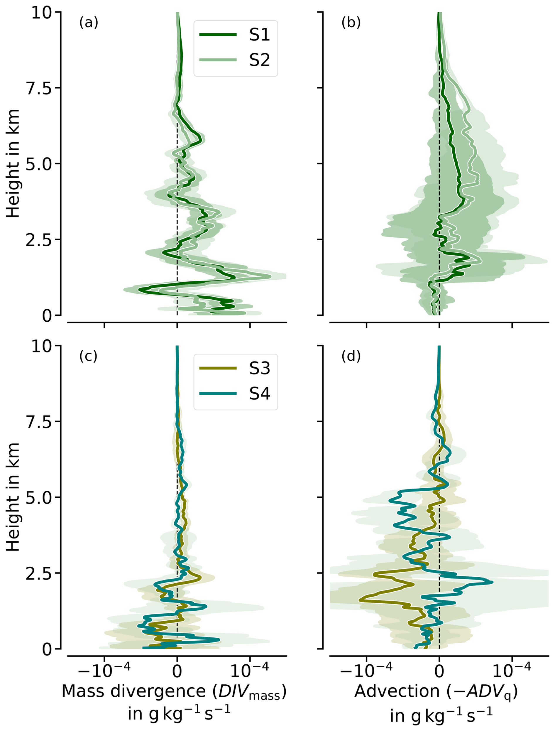
Figure 11 Vertical profiles of sonde-based moisture advection (negatively defined) and mass divergence for each of the pre-frontal AR corridors (S1–S4). The shadings indicate the uncertainties of the components based on the accuracy of the regression fits. For better visibility, values above 10 km are not considered due to their very minor contribution to ∇ ⋅ IVT.

For ADV_q, the dropsondes imply that the vertical characteristics undergo significant changes as well, though to a lesser extent within the marine boundary layer (<1 km). Despite the high moisture content, the marine boundary layer is well mixed, making advection a less dominant mechanism. During RF05 (Fig. 11b), dry advection prevails throughout the vertical profile on average, except for minor moisture advection around 2.5 km and in the marine boundary layer. Dry advection in mid-levels (3–7 km) intensifies notably from S1 to S2 but disappears during the second flight day (S3 and S4). In S3, moisture advection peaks in lower levels ($-\mathrm{1}\times {\mathrm{10}}^{-\mathrm{4}}{\mathrm{g}\mathrm{kg}}^{-\mathrm{1}}{\text{s}}^{-\mathrm{1}}$ at about 2 km), while being negligible in the mid- and upper levels (Fig. 11b, d). S4 shows significant moisture advection in the upper mid-levels (−0.5$\times {\mathrm{10}}^{-\mathrm{4}}{\mathrm{g}\mathrm{kg}}^{-\mathrm{1}}{\text{s}}^{-\mathrm{1}}$ at 5 km), above dry advection around 2.5 km. However, all derived ADV_q values are subject to larger uncertainties than those of DIV_mass due to spatial moisture variability, and they increase with larger sonde spacing during RF06. Particularly, in S4 just below 2.5 km, the limited number of sondes (four) leads to an uncertainty range of approximately $\pm \mathrm{1.5}\times {\mathrm{10}}^{-\mathrm{4}}{\mathrm{g}\mathrm{kg}}^{-\mathrm{1}}{\mathrm{s}}^{-\mathrm{1}}$ between dry and moisture advection. This variance contributes to the large uncertainty range in the integrated budget contribution of IADV_q (Fig. 10). Dropsondes from both flights indicate a very moist troposphere (not shown). Notably, the lower levels of the inflow cross-sections (up to 3 km) in S3 and S4 are much moister than S1 and S2. The highest q values are found in the marine boundary layer with 5 g kg⁻¹ for RF06, attributed to moisture accumulation from intensified IVT in the AR remnants west of the Norwegian coast (Fig. 8d). The trends in moisture transport divergence raise the question of how the cloud and precipitation fields respond.

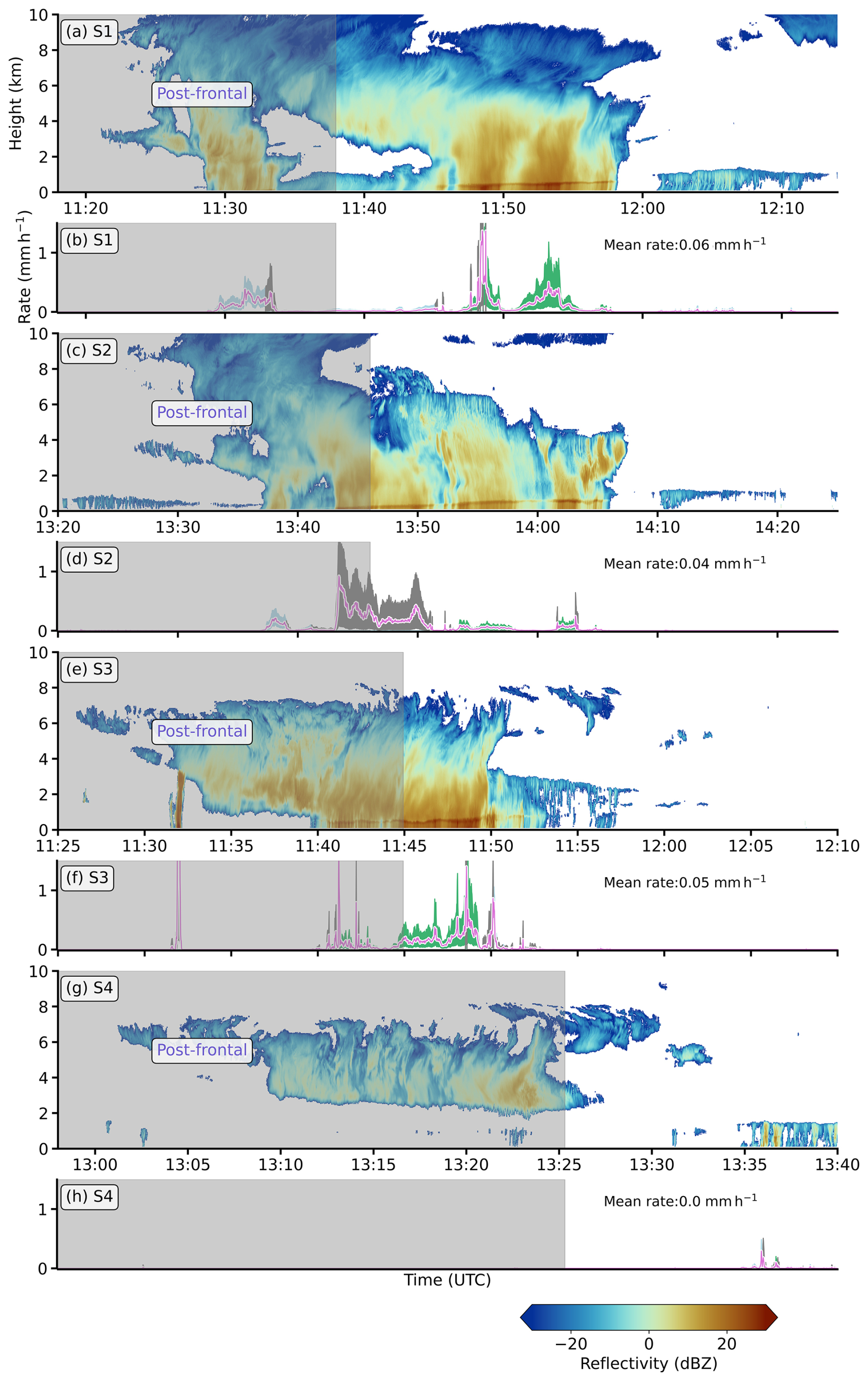
Figure 12 Radar-based cloud and precipitation fields of the four complete AR internal flight legs transecting the corresponding sectors S1–S4. Radar reflectivities (a, c, e, g) are shown with retrieved precipitation rates for snow (blue) and rain (green) resulting from our set of Z-R and Z-S relationships in (b, d, f, h), as well as the mean (pink). Uncertain phases (grey) consider both types of relationships. Coloured contours show the spread between the relationships. The grey-shaded areas on the left correspond to the post-frontal western part of the internal legs.

4.5 Trends in precipitation and cloud fields

Radar observations of the AR sectors indicate substantial changes in surface precipitation characteristics and cloud fields across the sectors (Fig. 12). Although precipitation overall contributes little to the moisture budget for all pre-frontal sectors in Fig. 10, it exhibits high spatial variability and differences between the sectors (Fig. 12). S1 shows moderate local precipitation rates of over 1 mm h⁻¹, mostly falling as rain with a melting layer at about 1 km. While the second pre-frontal sector (S2) has much weaker precipitation, S3 exhibits higher rates, again with a more heterogeneous convective structure. Convection triggering is consistent with the sonde-based mass convergence in S3 (Fig. 11c). Despite similar low-level mass convergence in S4, substantial advection of dry and unsaturated air at a height of 2 km (Fig. 11d) here appears to hinder cloud formation and precipitation. The full internal legs reveal that precipitation in the post-frontal (cold) sector is mainly snow.

For S1 and S2, the AR embedded precipitating deep clouds reach up to 12 km. While the internal leg belonging to S1 shows two major cloud filaments (Fig. 12a), these filaments have merged during S2. The high cloud tops during RF05 persist in a subsiding and drying environment, presumably causing the clouds to dissolve slightly towards RF06. For the second day, the deeper clouds do not reach above 8 km. The lowering of the clouds coincides with the decreasing depth of vertical mixing (Fig. 11d) when the higher troposphere (≥8 km) exhibits a dynamical equilibrium. For S4, the cloud systems decouple from the boundary layer, with a cloud base height between 2 and 4 km and a low cloud fraction underneath.

Summarising the trends of the budget components, we conclude that the IVT decay is not dominated by drying in lower levels but by a weakening of the winds. This weakening implies less spatial variability, resulting in lower mass divergence amplitudes and a reduced depth of vertical mixing and shallower cloud fields. The moisture transport divergence during RF05 is consistent with the directional dispersion of the IVT fields over the flight pattern (Fig. 8), leading to decreasing AR intensity and local drying. However, we neglected whether the components based on airborne observations robustly closed the moisture budget. If we aim to unravel air mass transformations within the AR by using the airborne budget components, we need to assess their plausibility by the magnitudes of emerging residuals in the budget closure of Eq. (1).

5 Plausibility of airborne perspective on budget components

5.1 Residuals in budget closure

We calculate the residuals from the difference between retrieved $\mathit{\delta }\mathrm{IWV}/\mathit{\delta }t$, based on HAMP measurements (Sect. 3.2), and the sum of all other airborne components contributing to $\mathit{\delta }\mathrm{IWV}/\mathit{\delta }t$ according to Eq. (1). Figure 13 shows that the mean residual for each sector is in the range of 0 to 1 mm h⁻¹, indicating that the residuals are within the range of the main moisture budget components. Except for S2, the mean residual concerning HAMP-based $\mathit{\delta }\mathrm{IWV}/\mathit{\delta }t$ results from a possible underestimation of sonde-based moisture transport divergence (IADV_q+IDIV_mass). S2 is notable for its high sonde-based moisture transport divergence, which, together with precipitation and condensation, overcompensates for the HAMP-based weak temporal water vapour change (drying). S2 is the only sector where the residual, together with its uncertainty range, is completely non-zero. For all other sectors, the moisture budget can be closed when the uncertainties of the budget components are included.

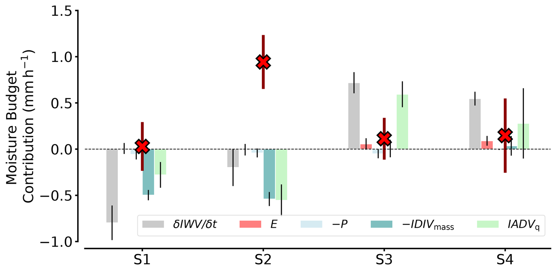
Figure 13 Residuals in airborne moisture budget closure for each pre-frontal AR sector (S1–S4). The residuals (red crosses) are shown with their uncertainties resulting from Gaussian error propagation of all budget component uncertainties. The bars repeat the values of all budget component contributions from Fig. 10 but are colour-coded paler.

Further investigation of the origins and causes of the residuals will improve the interpretation of the plausibility of the airborne budget components. The following analysis of the residuals compares our airborne budget components with those from the ICON-2km and ERA5 model grid data (Sect. 2.2). The models serve as a valuable tool to examine factors influencing the airborne representation. By leveraging the models, we can test the sensitivity of the airborne budget components concerning sonde-based sampling frequency and the nonstationarity of the AR, and we can investigate the airborne representativeness for the entire enclosed AR area. We use S1 as an example to assess the extent to which the airborne derivation and perspective of the budget components may differ from the actual prevailing components.

5.2 Sonde-based representativeness of IVT divergence

While sonde-based IVT provides high accuracy at individual points, the sporadic release of sondes leads to undersampling of moisture transport fields along the cross-sections, impacting the derivation of moisture transport divergence (Ralph et al., 2017; Dorff et al., 2024b). We compare sonde-based moisture transport divergence (Fig. 14; green) with the model-based values from ICON-2km, collocated along the flight path and analysed at the sonde locations (Fig. 14; grey). For the along-track perspective, the model-observation comparison shows good agreement. The profiles generated by ICON at the sonde locations show similarity in moisture transport divergence (ADV_q and DIV_mass) with the actual sonde-based profiles. The vertical variability is higher in the sonde-based profiles. In particular, the significant mass convergence within the LLJ evident from the sondes is not adequately reflected by the ICON-2km mimicked sondes (Fig. 14a). Nonetheless, the ICON-2km mimicked sondes and the real dropsondes show similar means of the integrated budget contributions, especially for IADV_q (Fig. 14).

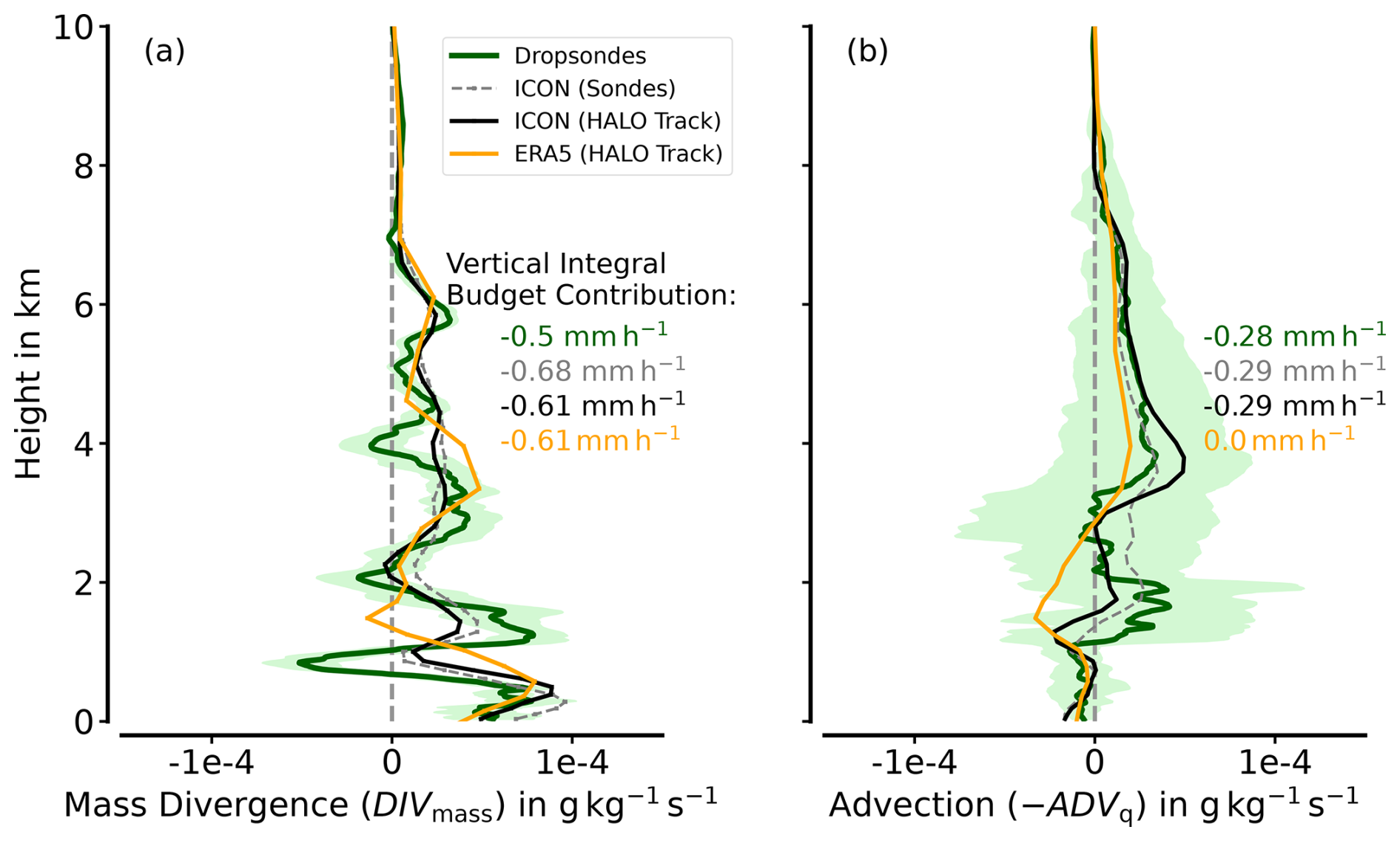
Figure 14 Along-track model-observation comparison of moisture transport divergence in S1. Sonde-based values are equivalent to those in Fig. 7. ICON values are interpolated onto the flight track and viewed in two resolutions: first, ICON-based moisture transport divergence is derived from wind and moisture data only at the sonde locations. Second, continuous sampling is mimicked along the AR cross-section legs. The latter represents the ideal sonde sampling for the flight pattern. For an easy view, ERA5 is only shown in the continuous representation.

Compared to the continuous along-track representation in ICON-2km (Fig. 14; black-bold), undersampling from discrete soundings has little effect on the divergence values for both composites, namely, ADV_q and DIV_mass. Differences in the moisture transport divergence between ICON values based on the sonde locations and those based on the continuous representation along the flight path are overall small, barely exceeding 0.1 mm h⁻¹ (Fig. 14). The largest discrepancies occur in ICON-based dry advection (below 3 km), which is overestimated when considering only the sonde locations (Fig. 14b). The uncertainties at each height are slightly lower for the continuous ICON-2km (not shown). We find that the continuously collocated ERA5 (Fig. 14; orange) has difficulties in representing the low-level moisture transport divergence below 3 km, as there are large deviations from ICON-2km and dropsondes. This confirms ICON-2km as a robust model-based IVT divergence along the flight track. The differences in ICON-based ∇ ⋅ IVT between the continuous and sporadic sonde release sampling strategies are too small to attribute the undersampling of moisture transport by sondes as the main cause for the residuals reaching up to 1 mm h⁻¹.

As a second effect, Dorff et al. (2024b) emphasise the temporal evolution of the AR, e.g. by AR displacement during flight, causing nonstationarity that represents a relevant source of error for sonde-based estimates of moisture transport divergence. In our AR case, both models reproduce stronger advection of moisture in the instantaneous view compared to the non-instantaneous observations (not shown). This stronger advection would, in turn, increase the residuals.

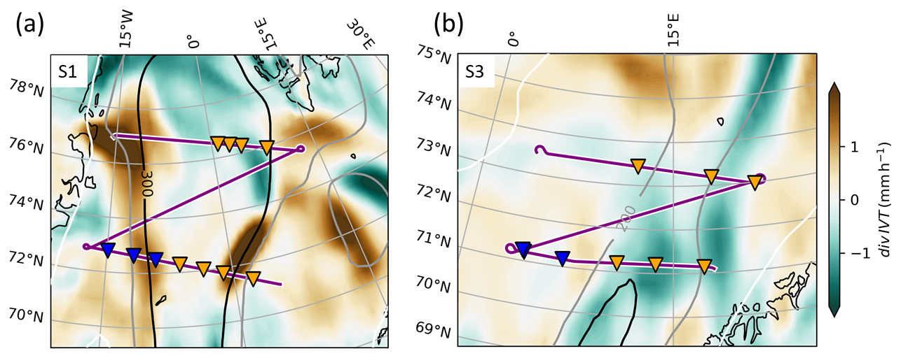
Figure 15 ERA5-based ∇ ⋅ IVT (colour-coded) for the centred hours of the zigzag patterns for S1 (a) and S3 (b). Flight tracks spanning the sectors and sondes (triangles) are superimposed (pre-frontal in orange; post-frontal in blue). Greyish contour lines show IVT in ${\mathrm{kg}\mathrm{m}}^{-\mathrm{1}}{\mathrm{s}}^{-\mathrm{1}}$.

Nonstationarity becomes most effective in deviating the airborne results when there is a high subscale spatial variability. Not only did the zigzag pattern take quite a long time, especially in RF05, but it also aimed to represent the divergence in a very large AR flight corridor. To further investigate the spatial variability of IVT divergence within the AR flight corridor, we examine the ERA5 moisture transport divergence field product, which is sufficient to capture the internal large-scale variability that may be missed by the airborne measurements. Figure 15a illustrates a pronounced dipole structure in the ERA5-based ∇ ⋅ IVT field within the pre-frontal sector of the AR flight corridor. While the southern region and the inflow leg exhibit divergence with budget contributions of ∇ ⋅ IVT ≤ −1 mm h⁻¹, the northern region is characterised by convergence and positive moisture rates of about 1 mm h⁻¹. This dipole is averaged out when the divergence calculations are based solely on the two cross-sections, resulting in lower airborne estimated budget contributions. An important factor for the divergence pattern in Fig. 15a is the widening of fields of strong IVT north of the inflow cross-section induced by changes in the transport (wind) direction (Fig. 2a). This change in wind direction within the flight corridor is reflected in the sonde-based predominance of DIV_mass against ADV_q. Furthermore, the dipole structure can clarify the along-track discrepancies between ICON-2km and ERA5. While the models are confident about the widening of strong IVT fields north of the ingoing leg, slight variations in the dipole pattern result in differing characteristics from the airborne perspective on ∇ ⋅ IVT. Thus, although the divergence calculations based on sonde data and the models align reasonably well along the flight path, their representativeness for the entire budget region is limited. In RF06, such dipole structures are absent (Fig. 15b). Instead, a more distinct zone of overall IVT convergence is identified. This indicates that the sampling in the AR flight corridors during RF06 is more representative despite fewer sondes.

5.3 Representativeness of airborne precipitation rates

The high precipitation rates due to this AR observed at Svalbard, with more than 30 mm d⁻¹ as reported by Walbröl et al. (2024), seem to contrast with the relatively low precipitation estimates along the AR flight corridor. However, the radar demonstrates the heterogeneity of precipitation within the AR, with local regions experiencing moderate precipitation (Fig. 6). This raises concerns regarding the representativeness of the airborne-radar-derived estimates. In particular, the curtain-based perspective of the radar may not capture the considerable variability in cloud conditions (Dorff et al., 2022). Additionally, the missing correction for hydrometeor radar attenuation is a limitation of the airborne estimates.

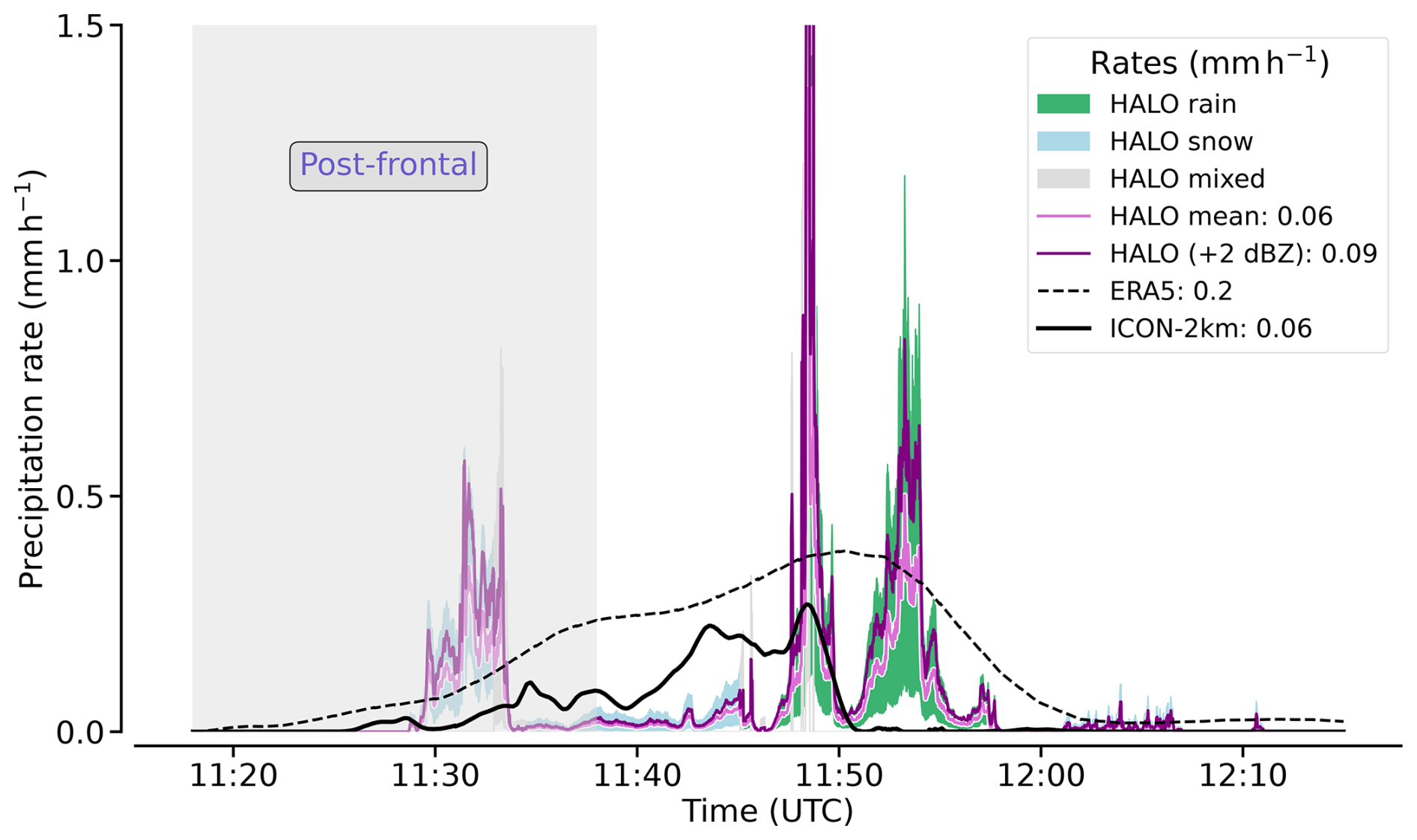
Figure 16 Precipitation rates along the internal flight leg of S1 (RF05). Shaded areas represent the uncertainty ranges arising from the minimum and maximum relationship values. Violet lines give mean radar precipitation. The darker line depicts precipitation rates based on simplified attenuation imitation (+2 dBZ). ICON and ERA5-based curves represent model precipitation along the flight track. Legend values yield the respective means of pre-frontal precipitation. The post-frontal part of the internal leg is presented but neglected in the mean.

Therefore, we revisit the comparison of the airborne data with the model data, focusing initially on precipitation from the along-track perspective. We compare the radar observations with the collocated ICON-2km and ERA5. Figure 16 shows the radar and the model data precipitation rates along the first internal leg belonging to S1. For the pre-frontal part of the internal leg, the mean precipitation of the along-track ICON-2km closely aligns with the radar-based precipitation estimates. At the same time, ERA5 shows significantly higher values in a few regions. ICON-2km shows greater fluctuations than ERA5 due to its finer horizontal resolution (Sect. 2.2), but it is much more homogeneous with lower spatial variability than the radar data. While ERA5 estimates a mean precipitation of 0.2 mm h⁻¹, its amplitude remains below 0.5 mm h⁻¹ and is even lower in ICON-2km. The two pre-frontal precipitation maxima seen in the radar data, with local rates exceeding 1 mm h⁻¹, are also found in ICON-2km, albeit with slight spatial shifts and smoothened with smaller local maxima.

The low radar-based precipitation mean could suggest an airborne underestimation, especially as the radar is uncorrected for hydrometeor attenuation. Specifically, the attenuation at the melting layer due to riming is mostly relevant. Li and Moisseev (2019) provide regression-based coefficients to quantify the attenuation by the melting layer and rain based on predetermined rain rates and reflectivities. We apply these coefficients to the rain rates in Fig. 16 and deduce a radar attenuation of up to 2 dBZ. To have a conservative estimate of the maximum underestimation of precipitation caused by attenuation, we thus increase all reflectivities by 2 dBZ. These elevated radar reflectivities increase the mean precipitation rate by 0.03 mm h⁻¹ (50 %) in Fig. 16. Radar-based precipitation estimates become more intense than that from ICON-2km, but ERA5 still indicates significantly stronger precipitation. Wang et al. (2019) also found that ERA5 tends to overestimate precipitation over the Arctic Ocean.

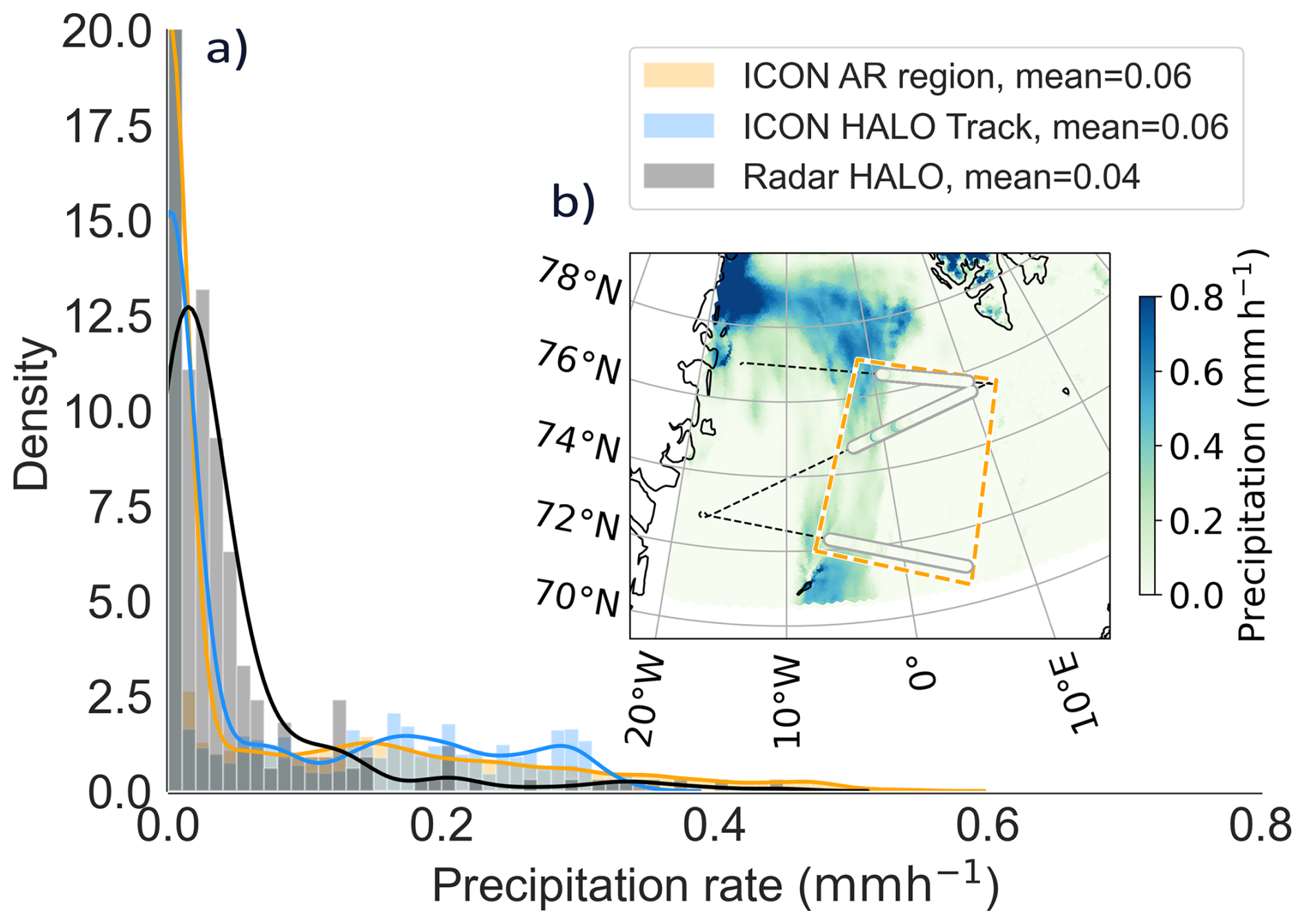
Figure 17 Kernel density estimate (KDE) of precipitation in the AR flight corridor of S1. Statistics refer to both the along-track precipitation rates and the rates for the entire AR flight corridor. (b) illustrates the spatial variability of ICON-based surface precipitation within the AR corridor for the ICON output at the centred flight hour. Airborne-radar-based precipitation rates are overlaid as colour-coded bold lines. The orange dashed rectangle (AR region) indicates the enclosed region of the pre-frontal AR sector S1 with which the aircraft collocated statistics are compared in (a). Background map made with Natural Earth.

Irrespective of attenuation effects, the high spatial variability of precipitation from the radar – and, to some extent, from ICON-2km – underscores the complexity of accurately representing precipitation conditions in an entire budget flight corridor using data from a single along-track curtain. Therefore, we compare the along-track distribution of precipitation rates with the horizontal distribution across the AR using the 2D surface field data from ICON-2km (Fig. 17). We average the radar reflectivities every 10 s to improve the comparability of the radar and ICON-2km data by achieving a similar horizontal resolution (≈2.5 km). Along the flight track, ICON reveals dominance of moderate precipitation rates ranging from 0.15 to 0.35 mm h⁻¹, while the radar locally shows higher rates. However, these higher rates are hardly relevant for the kernel density estimate (KDE) in Fig. 17a, which is why the radar still has a lower mean.

When incorporating the horizontal ICON precipitation field, both the KDE and the spatial precipitation pattern (Fig. 17a, b) show that the flight path misses several precipitation regions within the AR flight corridor. The northern area of the AR corridor has stronger precipitation that is underrepresented by the airborne radar. Over the flight corridor area, the precipitation rate KDE (Fig. 17a; orange) more greatly resembles a Weibull distribution, but higher precipitation rates contribute more than in the radar (Fig. 17a). Note that the spatial shift of the precipitation rates along the track in Fig. 17b is attributed to the temporal variations in AR dynamics during the zigzag manoeuvre, contrasting with the instantaneous model depiction.

Concluding the plausibility analysis of Sect. 5, we find a considerable subscale variability in the budget components within the AR flight corridors. Combined with the curtain-based sampling, this variability largely accounts for the residuals in the airborne budget closure. Our airborne analysis reveals that precipitation within Arctic ARs is hard to quantify. Even if precipitation is rather weak over the ocean, there is considerable small-scale precipitation variability. Future research efforts can expand upon the comparison between model-derived and observed precipitation using the remaining AR flight segments of HALO-(𝒜𝒞)³ (Walbröl et al., 2024; Wendisch et al., 2024).

6 Conclusions

This study provides comprehensive observational reference data that complement reanalyses and climate models to characterise the evolution of the moisture budget components in an Arctic atmospheric river (AR). The High-Altitude and LOng-Range Research Aircraft (HALO) sampled an intense Arctic AR, traversing the Greenland and Norwegian seas towards the Arctic sea ice. From the airborne measurements, we developed and applied methods to derive all major atmospheric moisture budget components in the Arctic AR and investigated four pre-frontal sectors (S1–S4) throughout the dissipation of the AR. We summarise the achievements of our research goals (G1–G3) as follows:

• To derive all moisture budget components in Arctic ARs from a research aircraft (G1). We show the feasibility of deriving the budget components using measurements from instruments on a single aircraft. Dropsondes released from zigzag flight patterns provide highly accurate profiling of moisture and wind at inflow and outflow cross-sections, with near-surface dropsonde data used for estimating evaporation. The dropsondes enable the calculation of moisture transport and thus IVT. Using training data from ERA5, a regression retrieval diagnoses IWV from brightness temperatures (TBs) measured by 25 microwave channels of an airborne radiometer. The results show good agreement with dropsonde data (RMSE < 0.5 kg m⁻²). The computationally efficient regression retrieval can be adapted to different training data from various regions; however, it is unsuitable for sea-ice-covered areas. Precipitation rates were estimated from nadir Ka-band radar reflectivities. Despite the high latitude and season, both rain and snow coexist in the AR. Omnipresent melting layers require attenuation estimates to correct the precipitation rates. To address uncertainties, we applied a set of Z-R/Z-S relationships.
  Although all airborne moisture budget components involve significant uncertainties, these remain smaller than the actual component magnitudes. This observational success, based on our zigzag flight strategy, facilitates future mission planning for airborne budget closure flights aimed at much-needed model-observation comparisons in the Arctic.

• To examine how the moisture budget components evolve during the dissipation phase of the AR (G2). Despite the AR dissipation due to IVT decay, the absolute magnitude of the moisture budget components remains relatively constant in the pre-frontal sectors. Within the Arctic AR, the components contribute to the moisture budget in a range of ±1 mm h⁻¹, slightly lower than what is found in mid-latitude ARs (Guan et al., 2020). The pre-frontal sectors (S1–S4) show a transition from local drying to moistening during AR dissipation. On the first day, a divergence due to the pressure field causes mass-divergent drying up to $-\mathrm{0.53}\pm \mathrm{0.07}{\mathrm{mm}\mathrm{h}}^{-\mathrm{1}}$ (S2), but heterogeneous precipitation and deep clouds resist the moisture transport divergence. On the second day, the convergence of moisture transport, primarily driven by moisture advection ($\mathrm{0.59}\pm \mathrm{0.14}{\mathrm{mm}\mathrm{h}}^{-\mathrm{1}}$, S3), leads to atmospheric moistening. For both days, the dropsondes indicate that the marine boundary layer maintains moisture with $q>\mathrm{4}{\mathrm{g}\mathrm{kg}}^{-\mathrm{1}}$, with mid-levels more influenced by advection.
  This case study highlights that local changes in IWV within the Arctic AR are primarily driven by moisture transport divergence via advection. This connection aligns with prior studies of pre-frontal moisture budget components in mid-latitude ARs (Cobb et al., 2021a; Guan et al., 2020) and emphasises the role of moisture transport in shaping regional Arctic moisture patterns (Nygård et al., 2020). Notably, the drying observed in the pre-frontal sectors (S1, S2) contrasts with patterns seen in mid-latitudes, where this sector is typically associated with moistening due to advection. The moist air masses within the Arctic AR exhibit weak surface interaction concerning precipitation and evaporation. However, the high spatial variability of precipitation complicates quantification in Arctic ARs. For the Arctic atmospheric water cycle, this study suggests that when AR moisture transport occurs over the Arctic Ocean, moisture is predominantly distributed in the atmosphere. Precipitation is marginal outside the AR core, particularly in the absence of strong moisture transport convergence or orographic forcing, causing reduced impacts on sea ice properties. The AR core is characterised more by a clustering of cellular plumes of precipitation than by a compact precipitation band.

• To assess how accurate and representative the airborne budget components are for the entire AR flight corridor (G3). The closure of the moisture budget using the mean airborne budget components results in significant residuals for all sectors, with magnitudes ranging from 0 to 1 mm h⁻¹, comparable to dominant budget components. Once uncertainties in the components are considered, the moisture budget can be closed for all sectors except S2. In comparison to model-based budget components mimicked along the flight, we find that the airborne values are realistic, consistently reflecting either drying or moistening throughout all sectors (not all shown) for both ICON-2km and ERA5. We note a sensitivity of ∇ ⋅ IVT values to the sonde spacing. However, in all sectors, sonde-based ∇ ⋅ IVT differs by less than 25 % from that of mimicked continuous sampling. The observed precipitation rates are in better agreement with ICON-2km than with ERA5, both in terms of mean values and variability across all sectors. While the airborne observations offer high spatial resolution for along-track precipitation and vertical variability of the moisture transport divergence, their spatial representativeness across the entire sector is limited. ICON-2km indicates that several precipitation fields tend to be located outside the internal flight legs. Additionally, even with an idealised continuous IVT sounding along the flight track, the subscale variability between the two cross-section legs remains significant (especially for ∇⋅ IVT in S1 and S2). This subscale variability underscores the limitations of the flight pattern, which hampers the closure of the airborne moisture budget when the meridional distance between cross-section legs is too great.

This study is limited to a single AR event. Nonetheless, our model-observation comparison already reveals both the limitations and strengths of each perspective. The observations provide insights into the AR moisture processes at an unprecedented spatial resolution. For example, the sonde-based moisture transport convergence at LLJ heights, which is poorly represented by the models, should be investigated across different AR events, as Dorff et al. (2024b) emphasise high case-to-case variability for Arctic ARs based on reanalyses. Such investigations will help substantiate the robustness of our findings regarding model-based misrepresentation of LLJ dynamics in Arctic ARs. This also applies to the significant precipitation variability observed by the radar, which is below the effective resolution of the model data for all sectors.

The closure of the moisture budget using HALO builds upon recent studies on airborne moisture budget components in mid-latitude ARs (e.g. Neiman et al., 2014; Norris et al., 2020). The uncertainty ranges of our residuals affirm the feasibility of the airborne moisture budget closure. Like Norris et al. (2020), we emphasise the importance of quantifying uncertainties for a robust observational moisture budget closure. From their values, we see a good agreement between our airborne budget components and the airborne-mimicked model representation, which underscores the reliability of our observational estimates. This feasibility provides significant potential for future airborne research on Arctic AR moisture budget components.

However, our airborne results are partially limited by reduced spatial representativeness, as significant subscale spatial variability is not captured by the flight curtain. Future flight patterns should retain the long cross-sections across the AR while reducing the distance between them. Shortening the meridional extent and flight duration may lessen the impact of nonstationarity, leading to improved divergence estimates. Dorff et al. (2024b) indicate that flight duration is more critical than sonde spacing for the misrepresentation of ∇ ⋅ IVT. This facilitates the verification of our observations in future airborne studies.

Furthermore, HALO-(𝒜𝒞)³ provides a wealth of data on Arctic ARs, particularly for characterising AR precipitation (e.g. Walbröl et al., 2024; Wendisch et al., 2024), analysed using the reanalyses in Lauer et al. (2023). The novel high-resolution C3S Arctic Regional Reanalysis (CARRA, Schyberg et al., 2021) can be evaluated with radar data. Another key research focus is the evolution and transformation of moist AR air masses during the ocean–sea ice transition. Our study lacks quasi-Lagrangian matches of air masses to compare the evolution of the budget components. Trajectory analyses for different AR events during HALO-(𝒜𝒞)³ indicate more frequent revisits of matching air masses (Ehrlich et al., 2025). However, these cases are complex for deriving the budget components due to limited sonde releases and the difficulty of retrieving IWV over sea ice. Such retrieval would facilitate comparisons of budget components across varying surface types, exploring whether AR air masses ascend over sea ice and examining the responses of moisture and clouds. Because our airborne study does not rely on additional observation platforms, we also recommend comparisons with spaceborne IWV fields in future studies. These perspectives for confronting airborne observations with additional data will provide greater clarity regarding the role of Arctic moist air intrusions by ARs, which are expected to increase in frequency and intensity in future climate scenarios (Kolbe et al., 2023).

Appendix A: Retrieval specifications

A1 Retrieval architecture and training data

The IWV is retrieved from the brightness temperatures (T_Bs) measured by the radiometer channels of the HAMP using a quadratic regression retrieval. For the frequency channels i, the regression relates measured T_Bi to IWV by:

$$\begin{array}{}\text{(A1)}& \mathrm{IWV}=\sum _i{a}_i\cdot T_{\mathrm{B},i}^{\mathrm{2}}+b_i\cdot T_{\mathrm{B},i}+c,\end{array}$$

with the regression coefficients a_i and b_i and the offset c. The Passive and Active Microwave TRAnsfer tool (PAMTRA; Mech et al., 2020) is used to create a synthetic training dataset to derive the regression coefficients for all HAMP channels at flight altitudes from 7 to 16 km with 200 m intervals. ERA5 fields of moisture, temperature, wind, hydrometeors, and surface properties for a domain over the North Atlantic (65 to 89° N, −30 to 50° E) and 100 random days from 1979 to 2020 are used as atmospheric input for PAMTRA. Nine AR events from Dorff et al. (2024b) containing IWV values up to 20 kg m⁻² were added to tune the training data for AR conditions. The entire training dataset focuses on atmospheric profiles over the open ocean only. The sea ice emissivity in the microwave spectrum is often unknown and very complex (Zabolotskikh and Azarov, 2022), with nonlinear masking effects on microwave T_Bs, making the retrieval of atmospheric properties over ice from microwave observations difficult. We conduct a least-squares fitting to the quadratic terms of the synthetic T_Bs and ERA5-IWV to obtain the retrieval coefficients in Eq. (A1).

A2 Retrieval performance

For the training data of ERA5-IWV and synthetic HAMP-TBs, the correlation coefficients range from 0.59 to 0.92 for the K-band channels, three V-band channels (51.76, 52.8, 53.75 GHz), and the F-band channels near the 118.75 GHz oxygen absorption line. Conversely, the G-band channels around 183 GHz exhibit a partially negative correlation because the warmer lower troposphere is concealed by mid- and upper tropospheric water vapour and due to cloud ice sensitivity. Thus, unlike the retrieval in Jacob et al. (2019), our retrieval incorporates all HAMP channels. This incorporation enables us to consider additional dependencies from the F-band channels and to address masking effects caused by hydrometeors at higher frequencies. To account for natural noise, all synthetic T_Bs have noise with a normal distribution and a standard deviation of 0.5 K for the K- and V-band and 1 K for the F-, W-, and G-band, following Mech et al. (2014). We conduct the least-squares fitting to the synthetic T_B values and ERA5-IWV to obtain the retrieval coefficients of Eq. (6), which we apply to the HAMP-TB measurements.

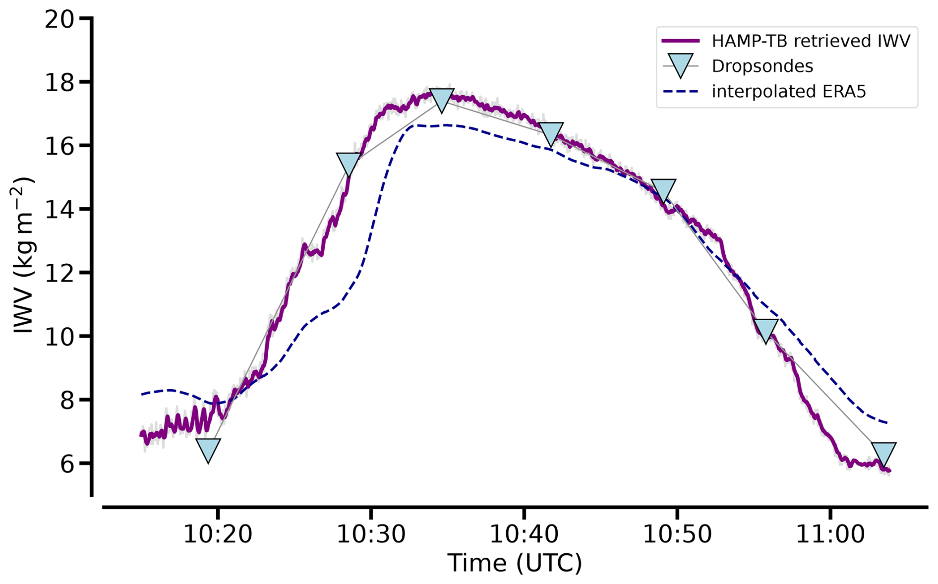
Figure A1 IWV along the first AR cross-section from RF05. Dropsonde-based IWV (triangles) are compared with the HAMP-based retrieved IWV (grey) that is smoothed using a 10 s running mean (purple). Aircraft collocated continuous ERA5-IWV is shown in blue.

To improve the comparability to dropsonde data, a 10 s running mean is applied to the HAMP retrieval output due to the noisy IWV retrieval values (Fig. A1). The retrieved IWV shows reasonable agreement with the dropsonde-based IWV over a wide range from 6 to 18 kg m⁻² (Fig. A1). Both airborne datasets show the bell-shaped curve of IWV commonly seen in AR cross-sections (Ralph et al., 2017). We derive a root-mean-square error (RMSE) of 0.42 kg m⁻² between retrieved IWV and sonde-based IWV, with the largest deviations at the highest IWV. For the sondes, George et al. (2021) report on a dry bias, but for HALO-(𝒜𝒞)³, a correction was not necessary because the sondes were reconditioned before flight (Ehrlich et al., 2025).

The comparison of the airborne-retrieved IWV values with the collocated and continuous ERA5-based representation (Sect. 2.2) confirms that the continuous HAMP representation reasonably replicates the IWV values. In particular, the cross-sectional IWV shape is very similar in ERA5 to the HAMP-retrieved IWV, with a steeper pre-frontal IWV increase against the post-frontal decline. In turn, the IWV amplitudes in ERA5 are lower and only reach up to 16 kg m⁻² (Fig. A1). Because ERA5 also shows lower values than the dropsondes, we conclude an underestimation of IWV in the reanalysis, where the sondes of these flights were not assimilated (Ehrlich et al., 2025). A slight shift is observed in the ERA5-based IWV representation, where the rapid increase in IWV occurs further east (3 min later than observed). However, we do not attribute this shift solely to a misrepresentation by the reanalysis but rather to the spatiotemporal interpolation between the hourly outputs of ERA5.