Influence of nitrogen oxides and volatile organic compounds emission changes on tropospheric ozone variability, trends and radiative effect

Ozone in the troposphere is a prominent pollutant whose production is sensitive to the emissions of nitrogen oxides (NO_x) and volatile organic compounds (VOCs). Here, we assess the variation of tropospheric ozone levels, trends, ozone photochemical regimes and radiative effects using the ECHAM6–HAMMOZ chemistry–climate model for the period 1998–2019 and satellite measurements. The global mean simulated trend in tropospheric column ozone (TRCO) for the study period (1998–2019) is 0.89 ppb decade⁻¹. During the overlapping period with Ozone Monitoring Instrument/Microwave Limb Sounder (OMI/MLS) observations (2005–2019), the simulated global mean TRCO trends (1.58 ppb decade⁻¹) show fair agreement with OMI/MLS estimates (1.4 ppb decade⁻¹). The simulations for doubling emissions of NO_x (DoubNO_x), VOCs (DoubVOC), and halving emissions of NO_x (HalfNO_x) and VOCs (HalfVOC) show nonlinear responses to ozone trends and tropospheric ozone photochemical regimes. The DoubNO_x simulations show VOC-limited regimes over the Indo-Gangetic Plain, eastern China, western Europe and the eastern US, while HalfNO_x simulations show NO_x-limited regimes over North America and Asia. Emissions changes in NO_x (DoubNO_x/HalfNO_x) influence the shift in tropospheric ozone photochemical regimes compared to VOCs (DoubVOC/HalfVOC).

The estimated global mean TO3RE during 1998–2019 from the control (CTL) simulations is 1.21 W m⁻². The global mean TO3RE shows enhancement by 0.36 W m⁻² in DoubNO_x simulations compared to CTL. While TO3RE shows a reduction in other simulations compared to CTL (DoubVOC: −0.005 W m⁻², HalfNO_x: −0.12 W m⁻² and HalfVOC: −0.03 W m⁻²). We show that emission changes in anthropogenic NO_x cause more significant changes in TO3RE than anthropogenic VOCs.

1 Introduction

Tropospheric ozone, a major air pollutant, has been a pressing issue in recent decades due to its detrimental effect on human health and ecosystem productivity and as a short-term climate forcer (Riese et al., 2012; Gulev et al., 2021; Wang et al., 2022). Considering these harmful impacts, the assessment of tropospheric ozone levels and trends is conducted frequently (Gaudel et al., 2018; Mills et al., 2018; Tarasick et al., 2019). Ozone trends are being assessed from surface observations, in situ and ground-based measurements, satellite retrievals, and model simulations (Cooper et al., 2014; Cohen et al., 2018; Young et al., 2018; Tarasick et al., 2019; Archibald et al., 2020). The latest Intergovernmental Panel on Climate Change Assessment Report (IPCC AR6) reported an enhancement in free tropospheric ozone by 2 %–7 % decade⁻¹ in the northern mid-latitudes, 2 %–12 % decade⁻¹ in the tropics and < 5 % decade⁻¹ in southern mid-latitudes (Gulev et al., 2021; Szopa et al., 2021). The Tropospheric Ozone Assessment Reports (TOARs) have documented global increases in tropospheric column ozone (TRCO) in the 20th century (Cooper et al., 2014; Lefohn et al., 2017; Schultz et al., 2017; Fleming et al., 2018; Gaudel et al., 2018; Mills et al., 2018; Young et al., 2018; Tarasick et al., 2019). Increasing tropospheric trends are explained by enhanced anthropogenic emissions (Cooper et al., 2014; Zhang et al., 2016) and modulation by climate variability (Lin et al., 2014; Lu et al., 2018). Several studies have documented increasing trends in TRCO across various regions and different time periods.

For instance, enhancement in TRCO trends globally using measurements from multiple sources such as In-service Aircraft for a Global Observing System database (IAGOS) and ozonesondes and GEOS–Chem model simulation revealed an increasing trend of 2.7 ± 1.7 and 1.9 ± 1.7 ppb decade⁻¹ between 1995 and 2017 (Wang et al., 2022). Additionally, Fiore et al. (2022) also found increasing trends ranging from 0.6 to 2.5 ppb decade⁻¹ from 1950 to 2014 globally based on the available limited surface ozone records and the Community Earth System, version-2, the Whole Atmosphere Community Climate Model, version-6 (CESM2–WACCM6), model study. Furthermore, trends in TRCO are stronger in the Northern Hemisphere (NH) than the Southern Hemisphere (SH) due to larger anthropogenic emissions (Monks et al., 2015). Ozone Monitoring Instrument (OMI) and Microwave Limb Sounder (MLS) observations from 2005 until 2010 show annual TRCO burden averaged over the NH exceeds the SH by 4 % at low latitudes (0–25°), by 12 % at mid-latitudes (25–50°) and by 18 % at high latitudes (50–60°) (Cooper et al., 2014). CMIP6 models also show that the tropospheric ozone burden increased by 44 % in 2005–2014 compared to 1850 (Griffiths et al., 2021). Recently, studies have reported a decrease in TRCO trends globally after the coronavirus disease 2019 (COVID-19) outbreak (e.g. Chang et al., 2022, 2023, and Steinbrecht et al., 2021). Also, Putero et al. (2023) show widespread ozone decreases at high-elevation sites due to the COVID-19 lockdown. However, our study period (1998–2019) excludes the COVID-19-associated emission changes.

Nitrogen oxides (NO_x; NO + NO₂) and volatile organic compounds (VOCs) are the major precursors that define ozone photochemical regimes (Duncan et al., 2010). Information on ozone photochemical regimes is of utmost importance to know ozone (O₃) levels. However, the nonlinearity in the O₃–NO_x–VOC chemistry has always posed a challenge in identifying photochemical regimes. The regime is called NO_x-limited if the ozone production is directly related to a change in NO_x rather than from VOC perturbations, whereas the region where ozone production is regulated by the ambient availability of VOCs is called VOC-limited (Sillman et al., 1990; Kleinman, 1994). The ratios such as of ozone to oxidised nitrogen species (O₃ / (NO_y – NO_x), where NO_y is the total reactive nitrogen), formaldehyde to total reactive nitrogen (HCHO $/$ NO_y), formaldehyde to nitrogen dioxide (HCHO $/$ NO₂) and hydrogen peroxide to nitric acid (H₂O₂ $/$ HNO₃) are adopted to diagnose the ozone photochemical regimes (e.g. Sillman, 1995; Martin et al., 2004; Duncan et al., 2010). Among these, the most widely used indicator to identify regimes is the formaldehyde-to-nitrogen dioxide (HCHO-to-NO₂) ratio (FNR) (Martin et al., 2004; Duncan et al., 2010). In our study, we adopt FNR to identify NO_x-limited or VOC-limited regimes. On par with the current effort to mitigate ozone pollution, it is important to understand how the changes in emissions of NO_x and VOCs affect the ozone photochemical regimes and trends (Jin et al., 2017, 2020).

Ozone is the third-strongest anthropogenic greenhouse gas, also called a short-term climate forcer, producing a global average radiative forcing of 0.47 [0.24 to 0.71] W m⁻² (5 % to 95 % uncertainty range) (Forster et al., 2021). Recent studies showed ozone effective radiative forcing (ERF) of 0.51 [0.25 to 0.76] W m⁻² during 1750–2023 (Forster et al., 2024). The knowledge of ozone radiative forcing due to changes in anthropogenic emissions of NO_x and VOCs will help to assess climate change. Therefore, we also show the impacts of enhanced or reduced emissions of NO_x and VOCs on ozone radiative effect in addition to ozone trends and photochemical regimes. To achieve this, we conducted sensitivity experiments by doubling and halving global NO_x and VOC emissions using the state-of-the-art chemistry–climate model ECHAM6–HAMMOZ for the period 1998–2019. This approach of increase/decrease in emissions is important to understand the nonlinear response of ozone to emission changes. These experiments are helpful for designing emission implementation strategies (e.g. Zhang et al., 2021; Wang et al., 2023). The paper is outlined as follows: satellite data and the model experimental setup are given in Sect. 2, and results are given in Sect. 3, which include a comparison of simulated tropospheric column ozone with satellite data and estimated ozone trends. Discussions on ozone photochemical regimes and their trends are made in Sects. 4 to 6. Estimates of ozone radiative effects are given in Sect. 7. Conclusions are made in Sect. 8.

2 Satellite data and model experiments

2.1 OMI satellite data

We include OMI/MLS tropospheric column ozone (TRCO) for October 2004–December 2019 and OMI NO₂ and HCHO data for the latitude range from 60° S–60° N (Ziemke et al., 2006; De Smedt et al., 2021; Lamsal et al., 2021). OMI/MLS TRCO is determined by subtracting MLS stratospheric column ozone (SCO) from OMI total column ozone each day at each grid point. Tropopause pressure used to determine the SCO invoked the World Meteorological Organization (WMO) 2 K km⁻¹ lapse-rate definition from the National Centers for Environmental Prediction (NCEP) reanalysis. The MLS data used to obtain SCO were derived from the MLS v4.2 ozone profiles. We estimate 1σ precision for the OMI/MLS monthly mean gridded TRCO product to be about 1.3 DU. Adjustments for drift calibration and other issues (e.g. OMI row anomaly) affecting OMI/MLS TRCO are discussed by Ziemke et al. (2019) and Gaudel et al. (2024).

We used OMI monthly mean Level-3 (L3) data for NO₂ and HCHO (https://doi.org/10.18758/h2v1uo6x, De Smedt et al., 2024a) that were produced in the context of the ESA CCI+ precursors for aerosols and ozone project (De Smedt et al., 2021; Anglou et al., 2024). The datasets consist of the monthly mean tropospheric column densities for NO₂ and HCHO (based on the QA4ECV NO₂ and HCHO dataset) as measured by OMI from October 2004 to March 2019 and include minimum spatial and temporal coverage thresholds (De Smedt et al., 2018). OMI has an overpass time of 13:30 local time, and the retrieved column densities concern clear-sky or partially cloudy conditions.

2.2 IASI-SOFRID

The Software for a Fast Retrieval of Infrared Atmospheric Sounding Interferometer (IASI) data (SOFRID) retrieves global ozone profiles from IASI radiances (Barret et al., 2011, 2021). It is based on the RTTOV (Radiative Transfer for TOVS) operational radiative transfer model jointly developed by ECMWF, Météo-France, UKMO and KNMI within the NWPSAF (Saunders et al., 1999; Matricardi et al., 2004). The RTTOV regression coefficients are based on line-by-line computations performed using the HITRAN2004 spectroscopic database (Rothman et al., 2005), and the land surface emissivity is computed with the RTTOV UW-IRemis module (Borbas and Ruston, 2010). The IASI-SOFRID ozone for the study period (2008 to 2019) is obtained from METOP–A (2008–2018) and METOP–B (2019).

We use the SOFRID version 3.5 data presented and validated in Barret et al. (2021), which use dynamical a priori profiles from an O₃ profile tropopause-based climatology according to tropopause height, month and latitude (Sofieva et al., 2014). The use of such an a priori has largely improved the retrievals, especially in the SH, where the previous version was biased. The retrievals are performed for clear-sky conditions (cloud cover fraction < 20 %). IASI-SOFRID ozone retrievals provide independent pieces of information in the troposphere, the UTLS (300–150 hPa) and the stratosphere (150–25 hPa) (Barret et al., 2021). SOFRID TRCO absolute biases relative to ozonesondes are lower than 8 % with root mean square error (RMSE) values lower than 18 % across the six 30° latitude bands (see Barret et al., 2021). Importantly, Barret et al. (2021) have shown that relative to ozonesondes, TRCO from IASI-SOFRID display no drifts (< 2.1 % decade⁻¹) for latitudes lower than 60° N and in the SH for latitudes larger than 30° (< 3.7 % decade⁻¹). But significant drifts are observed in the SH tropics (−5.2 % decade⁻¹) and in the NH at high latitudes (12.8 % decade⁻¹).

2.3 IASI + GOME2

IASI + GOME2 is a multispectral approach to retrieving the vertical profile of ozone and its abundance in several partial columns. It is based on the synergy of IASI and GOME2 spectral measurements in the thermal infrared and ultraviolet spectral regions, respectively, which are jointly used to improve the sensitivity of the retrieval for the lowest tropospheric ozone (below 3 km a.s.l.; see Cuesta et al., 2013). Studies over Europe and East Asia have shown particularly good capabilities for capturing near-surface ozone variability compared to surface in situ ozone measurements (Cuesta et al., 2018, 2022; Okamoto et al., 2023). TRCOs from IASI-GOME2 also show good agreement with several datasets of in situ measurements for a 4-year period in the tropics with almost negligible biases and high correlations (Gaudel et al., 2024). This ozone product provides global coverage for low-cloud-fraction conditions (below 30 %) for 12 km diameter pixels spaced 25 km apart (at nadir). The IASI-GOME2 global dataset is publicly available through the French AERIS data centre, with data from 2017 to the present, and covers the 90° S–90° N latitude band. For this study, we use the monthly TRCO data between the surface and the tropopause for 2017–2019 for different latitude bands.

2.4 TROPOMI

The TROPOspheric Monitoring Instrument (TROPOMI) is the sole payload on the Copernicus Sentinel-5 Precursor (Sentinel-5P or S5P) satellite, which provides measurements of multiple atmospheric trace species, including NO₂ and HCHO, at high spatial and temporal resolutions (Veefkind et al., 2012). TROPOMI has a daily global coverage with a spatial resolution of 5.5 × 3.5 km² at nadir since a long-track pixel size reduction on 6 August 2019. We have used the ESA CCI+ Level-3 gridded 1° × 1° monthly tropospheric column of NO₂ (based on L2 v2.3.1, which applies a retrieval consistent with the most recent TROPOMI L2 version) and HCHO (https://doi.org/10.18758/2imqez32, De Smedt et al., 2024b) (based on L2 v2.4.1, collection 3) data from May 2018 to December 2019 for our study (De Smedt et al., 2021; Glissenaar et al., 2024). This dataset was created using the same methods as the ESA CCI+ OMI Level-3 datasets.

2.5 The ECHAM6–HAMMOZ model experiments

The ECHAM6.3–HAM2.3–MOZ1.0 aerosol chemistry–climate model (Schultz et al., 2018) used in the present study comprises the general circulation model, ECHAM6 (Stevens et al., 2013); the tropospheric chemistry module, MOZ (Stevenson et al., 2006); and the aerosol module, Hamburg Aerosol Model (HAM) (Vignati et al., 2004). The gas-phase chemistry is represented by the Jülich Atmospheric Mechanism (JAM) v002b mechanism (Schultz et al., 2018). This scheme is an update and an extension of terpenes and aromatics oxidation based on the MOZART-4 model (Emmons et al., 2010) chemical scheme. Tropospheric heterogeneous chemistry relevant to ozone is also included (Stadtler et al., 2018). MOZ uses the same chemical preprocessor as CAM-Chem (Lamarque et al., 2012) and WACCM (Kinnison et al., 2007) to generate a FORTRAN code containing the chemical solver for a specific chemical mechanism. Land surface processes are modelled with JSBACH (Reick et al., 2013). Biogenic VOC emissions are modelled with the MEGAN algorithm (Guenther et al., 2012), which has been coupled with JSBACH (Henrot et al., 2017). The lightning NO_x emissions are parameterised in ECHAM6–HAMMOZ as described by Rast et al. (2014). The lightning parameterisation is the same in all the simulations. The model simulations were performed for the period 1998 to 2019 using the Atmospheric Chemistry and Climate Model Intercomparison Project (ACCMIP) (Lamarque et al., 2010; Van Vuuren et al., 2011) emission inventory. The ACCMIP emission inventory includes emissions from agriculture and waste burning, forest and grassland fires, aircraft, domestic fuel use, energy generation including fossil fuel extraction, industry, ship traffic, solvent use, transportation, and waste management.

The model was run at a T63 spectral resolution corresponding to about 1.8° × 1.8° in the horizontal dimension and 47 vertical hybrid σ p levels from the surface up to 0.001 hPa. The details of model parameterisations and validation are described by Fadnavis et al. (2019b, a, 2021b, a, 2022, 2023). We performed five experiments: (1) control (CTL) and four emission sensitivity experiments: (2) doubling anthropogenic emission of NO_x globally (DoubNO_x), (3) reducing anthropogenic emissions of NO_x by 50 % globally (HalfNO_x), (4) doubling anthropogenic emissions of all VOCs globally (DoubVOC), and (5) reducing anthropogenic emissions of all VOCs by 50 % globally (HalfVOC). We performed each experiment from 1998 to 2019 after a spin-up of 1 year. We used the Representative Concentration Pathway (RCP) 8.5 high-emission scenario (Van Vuuren et al., 2011) in all model simulations. In each experiment, the monthly varying AMIP-II sea surface temperature and sea ice representative of the period 1998–2019 were specified as a lower-boundary condition. Anthropogenic VOC emissions included in the model are listed in Table S1 in the Supplement.

TRCO is computed from the satellite data and model simulations by averaging O₃ amounts from the surface up to the tropopause. The partial tropospheric column is converted into a mixing ratio assuming a constant ozone mixing ratio in the troposphere. Tropopause considered is as described by the WMO thermal tropopause definition, the lowest level at which the temperature lapse rate decreases to 2 K km⁻¹ or less (WMO, 1957). The estimated tropopause in the satellite data will show differences since the tropopause is quite variable in space and time; its location will depend on the employed reanalysis (e.g. Hoffmann and Spang, 2022). The vertical resolution of the satellite and the ECHAM6–HAMMOZ also affect the estimated tropopause. For comparison of the model with satellite datasets (e.g. IASI-SOFRID and OMI/MLS), we use model and satellite data for the same period.

2.6 Tropospheric ozone radiative effects

The tropospheric ozone radiative effect (TO3RE) is calculated as in Pope et al. (2024). While the radiative effect calculated in ECHAM6–HAMMOZ also includes impacts of aerosols and dynamical effects, here we isolate TO3RE using the Rap et al. (2015) tropospheric ozone radiative kernel derived from the SOCRATES offline radiative transfer model (Edwards and Slingo, 1996), including stratospheric temperature adjustments. To calculate the TO3RE, the monthly averaged ECHAM6–HAMMOZ simulated ozone field is multiplied by the offline radiative kernel (at every grid box). It is then summed from surface to the tropopause. The simulated ozone data are mapped onto the spatial resolution of the radiative kernel and then interpolated vertically onto its pressure grid. The equation for each grid box is

$$\begin{array}{}\text{(1)}& \mathrm{TO}\mathrm{3}\mathrm{RE}=X{\mathrm{trop}}_i={\mathrm{surfRK}}_i\times {\mathrm{O}}_{\mathrm{3}i}\times \mathrm{d}{p}_i/\mathrm{100},\end{array}$$

where TO3RE is the tropospheric ozone radiative effect (W m⁻²), RK is the radiative kernel (W m⁻² ppbv⁻¹ 100 hPa⁻¹), O₃ is the simulated ozone grid box value (ppbv), dp is the pressure difference between vertical levels (hPa) and “i” is the grid box index between the surface pressure level and the tropopause pressure. The tropopause pressure is identified based on the WMO lapse-rate tropopause definition. Several past studies have used this approach of using the SOCRATES offline radiative kernel with output from model simulations to derive the TO3RE (Rap et al., 2015; Scott et al., 2018; Rowlinson et al., 2020; Pope et al., 2024).

3 Results

3.1 Comparison of the simulated seasonal cycle in TRCO, NO₂ and HCHO with satellites retrievals

In this section, we compare the estimated TRCO from the model (CTL) simulation with OMI/MLS (2005–2019), IASI-SOFRID (2008–2019) and IASI-GOME2 (2017–2019) satellite retrievals. We compared simulated TRCO for the same period as individual satellite retrievals. The comparison of monthly mean TRCO is made for 20° latitude bins in Fig. 1. In the northern tropics (0–20° N) (Fig. 1a), the OMI/MLS data exhibit an annual cycle with a peak in April, whereas the model indicates a peak in January. Both datasets show a minimum in August. The model underestimates TRCO by 1.8 to 3.9 ppb during March to October. In the 21–40 and 41–60° N latitude bands (Fig. 1b–c), the model shows a 1-month lead in the peak of the annual cycle compared to OMI/MLS. In the 21–40° N band, the model underestimates OMI/MLS TRCO by 2.8–6.1 ppb during the summer months (May–August), while it overestimates TRCO by 4.1–8.3 ppb from October to March. The 41–60° N latitude band exhibits an underestimation in the model by 1.1–6.3 ppb during June and July, while it overestimates (0.7–7.5 ppb) the rest of the year. In the Southern Hemisphere (SH), OMI/MLS and the model show a similar pattern in the seasonal cycle. The model shows a 1-to-2-month lead in the annual cycle. However, the model shows an underestimation of TRCO for all months. The model underestimates TRCO by 0.5 to 7.1 ppb in the 0–20 ° S, by 5.1–15.3 ppb in the 21–40° S and by 9.2–13.8 ppb in the 41–60° S latitude bands. The comparison of TRCO from IASI-SOFRID with the model shows features similar to those in the OMI/MLS. In the 0–20° N latitude band, the model underestimates the TRCO by about 3.8 to 7.7 ppb from April to October and in the 21–60° N latitude band by 1.9–11.3 ppb in summer (May–August). In the SH, the model shows better agreement with IASI-SOFRID than OMI/MLS. During the SH winter (June–August), the model overestimates TRCO by 2.8–6.5 ppb in the latitude range of 0–40° S. Conversely, it underestimates TRCO by 2.7–8.2 ppb in the 41–60° S throughout the year, which is less compared to other satellite datasets. IASI-SOFRID is known to suffer from negative drifts in the SH (Barret et al., 2021).

Interestingly, the model exhibits a fair agreement with IASI-GOME2 retrieved TRCO during the summer months (May–August) in the Northern Hemisphere (NH). During the winter months, the estimated TRCO shows a large overestimation of 8.3–11.7 ppb in the NH (0–40° N), while it is underestimated by 8.3–11.7 ppb in the 41–60° N. In the SH, a fairly good agreement is observed between the model and IASI-GOME2 TRCO, especially in the 0–40° S latitude band. The model overestimates the TRCO by 7.4–8.8 ppb in the 0–20° S during SH winter and underestimates it by 4.7–6.7 ppb in the 21–40° S belt during SH summer (December, January, February). An overall underestimation of about 7–11.2 ppb in TRCO is noted in the 41–60° S throughout the year. Figure 1 shows that a peak in the seasonal cycle in the model is earlier than the three satellite data between 40° N and 40° S. In general, the model underestimates TRCO in summer in the NH and overestimates it in winter relative to OMI/MLS and IASI-SOFRID. In the SH, the model underestimates TRCO throughout the year compared to OMI/MLS, IASI-SOFRID and IASI-GOME2, especially in the 41–60° N band. Although the model–satellite comparison is done for the same period, the differences in sampling between the model and satellite measurements may cause the observed differences. It should be noted that the spatial resolution, coverage and diurnal sampling time differ among the satellites, which also contribute to the observed differences among them.

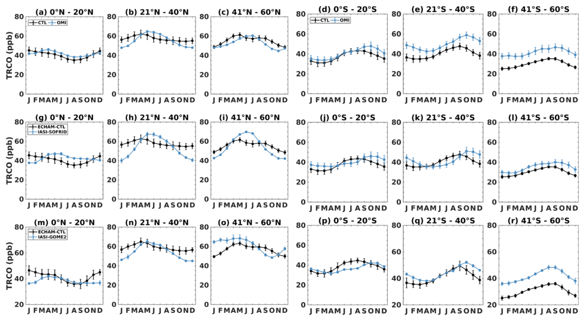
Figure 1 Time series of monthly mean TRCO (ppb) averaged for 20° wide latitude bins from (a–f) OMI/MLS (blue) and ECHAM6–HAMMOZ CTL simulations (black) for the time period from October 2004–December 2019. (g–l) Same as (a)–(f) but for IASI-SOFRID (blue) and ECHAM6–HAMMOZ CTL simulations (black) for the period January 2008–December 2019, and (m–r) the same as (a)–(f) but for IASI-GOME2 (blue) and ECHAM6–HAMMOZ CTL simulations (black) for the time period from January 2017–December 2019. The vertical bars in all the figures represent 2σ standard deviation.

To evaluate our model simulations of NO₂ and HCHO, we compare the simulated tropospheric column NO₂ and HCHO with the ESA CCI+ monthly averaged TROPOMI and OMI data (Fig. 2). The simulated NO₂ reproduces the seasonal cycle but shows overestimation in the entire latitude band except 41–60° S in the SH. In the NH, the magnitude of overestimation in the simulated NO₂ increases with latitude. Simulated NO₂ is overestimated by 0.15 to 0.35 × 10¹⁵ molec. cm⁻² in the 0–20° N, by 0.3 to 0.6 × 10¹⁵ molec. cm⁻² in the 21–40° N and by 0.25 to 0.9 × 10¹⁵ molec. cm⁻² in the 41–60° N latitude bands compared to TROPOMI. Similarly, simulated NO₂ is overestimated compared to OMI by 0.16 to 0.35 × 10¹⁵ molec. cm⁻² in the 0–20° N, by 0.16 to 0.48 × 10¹⁵ molec. cm⁻² in the 21–40° N and by 0.18 to 0.76 × 10¹⁵ molec. cm⁻² in the 41–60° N latitude belts (Fig. 2a–c and g–i). Although the model overestimates NO₂ in the SH, the magnitude of this overestimation is smaller compared to NH. Simulated NO₂ shows a fairly good agreement from 21 to 60° S latitudes in the SH (Fig. 2d–f and j–l).

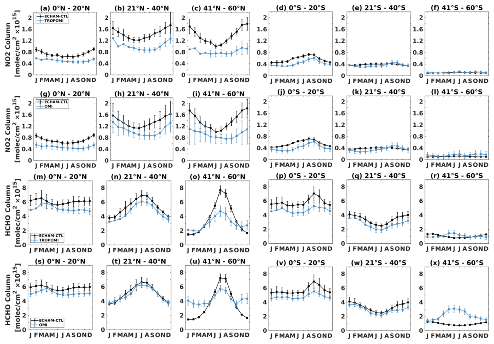
Figure 2 Time series of monthly mean tropospheric column NO₂ (molec. cm⁻²) averaged for 20° wide latitude bins from ECHAM6–HAMMOZ CTL simulations (black) for the same time period as (a–f) TROPOMI from May 2018 to December 2019 and (g–l) OMI from January 2005 to December 2019. Panels (m)–(x) are the same as (a)–(l) but for HCHO. The vertical bars in the figures represent 2σ standard deviation.

While the simulated HCHO successfully reproduces the seasonal cycle in both hemispheres, it shows a large overestimation, particularly in the tropical region (Fig. 2m–x). The overestimation is most pronounced when compared to TROPOMI, especially in the tropics, and to a lesser extent with OMI. The model HCHO aligns reasonably well with both TROPOMI and OMI in the northern and southern mid-latitudes (21–40° N and 21–40° S) with a modest overestimation of 0.4–1.2 × 10¹⁵ and 0.3–0.5 × 10¹⁵ molec. cm⁻², respectively, in the NH and 0.4–1 × 10¹⁵ and 0.5–1.4 × 10¹⁵ molec. cm⁻², respectively, in the SH. However, in the 41–60° N band, the model overestimates HCHO compared to TROPOMI (OMI) by 0.6–2.9 (0.5–1.7) × 10¹⁵ molec. cm⁻² during the NH from May to October and underestimates it by 0.08–1.1 (0.01–2.7) × 10¹⁵ molec. cm⁻² during other months. On the contrary, the model underestimates HCHO in the 41–60° S during SH winter. It should be noted that TROPOMI/OMI monthly means are valid for clear-sky situations, whereas the model simulations are all-day all-sky averages. In previous studies (Boersma et al. (2016) and references therein), it was shown that NO₂ is typically 15 %–20 % lower on clear-sky days than in cloudy situations due to higher photolysis rates and faster chemical loss of NO₂. Further, OMI and TROPOMI cannot sample for snowy scenes and nighttime. There is significantly lower coverage on the NH during winter and vice versa for SH. These all can likely cause model and satellite differences. For HCHO, the effect is smaller because HCHO is both produced and destroyed by OH (see Fig. 4 in Boersma et al., 2016). In addition, diurnal NO₂ observations from Geostationary Environment Monitoring Spectrometer (GEMS) (Edwards et al., 2024) showed that the tropospheric column diurnal NO₂ variations can be larger than 50 % of the column amount compared to once-a-day TROPOMI observations. Considering these differences, we proceed with the analysis of TRCO trends, ozone photochemical regimes and ozone radiative effects.

3.2 Impacts of emission changes on the spatial distribution of ozone

Figure 3 shows the spatial distribution of the simulated surface (Fig. 3a–e) and TRCO (Fig. 3f–j) concentration from ECHAM CTL simulations and the anomalies obtained from differences in DoubNO_x – CTL, DoubVOC – CTL, HalfNO_x – CTL and HalfVOC – CTL simulations for the period 1998–2019. The CTL simulation shows high surface ozone levels (19–61.1 ppb) between 10–40° N (Fig. 3a). Doubling of NO_x emission (DoubNO_x) causes a global mean enhancement of surface ozone anomalies by 4.1 [−3.8 to 13] ppb (5th to 95th percentile). Surface ozone anomalies show an increase of 5–20 ppb across most of the globe, excluding highly urbanised regions such as the Indo-Gangetic Plain (IGP), Southeast China, northeastern United States (US) and Europe. (Fig. 3b). Over these regions, a large reduction (8–20 ppb) in surface ozone anomalies is noticed, indicating ozone titration by NO_x. While surface ozone anomalies from DoubVOC – CTL simulations show global mean enhancement by 0.9 [0.1 to 2.3] ppb, its magnitude is less than that of the anomalies from DoubNO_x – CTL (Fig. 3c). The largest increase in surface ozone anomalies for DoubVOC is observed over the IGP, eastern China and eastern US (3–6 ppb). Interestingly, these are the same regions where a decrease in ozone anomalies is observed in the DoubNO_x case. The decrease (increase) in ozone anomalies with an increase in NO_x (VOC) emissions indicates that these regions could be NO_x-saturated or VOC-limited. Reduction in NO_x emissions (HalfNO_x – CTL) simulations show a reduction in surface ozone anomalies (global mean by −2.5 [−7.2 to −0.7] ppb) except over northeastern China (Fig. 3d). Earlier, Souri et al. (2017) also reported that eastern Asia has witnessed a rise in surface ozone levels despite NO_x control strategies, indicating the prevalence of VOC-limited photochemistry over this region (details in Sects. 4 to 6). However, the absence of such an increase over other VOC-limited regions point toward nonlinear ozone chemistry. While the HalfVOC – CTL stimulation causes a reduction in surface ozone anomalies (global mean by −0.4 [−1.4 to 0.05] ppb), an increase is observed in South America, some parts of the US, Australia and the former Indo-China Peninsula (Fig. 3e). This increase could be due to a reduction in the radical destruction of ozone caused by aromatic hydrocarbons in low NO_x conditions in these regions (Taraborrelli et al., 2021).

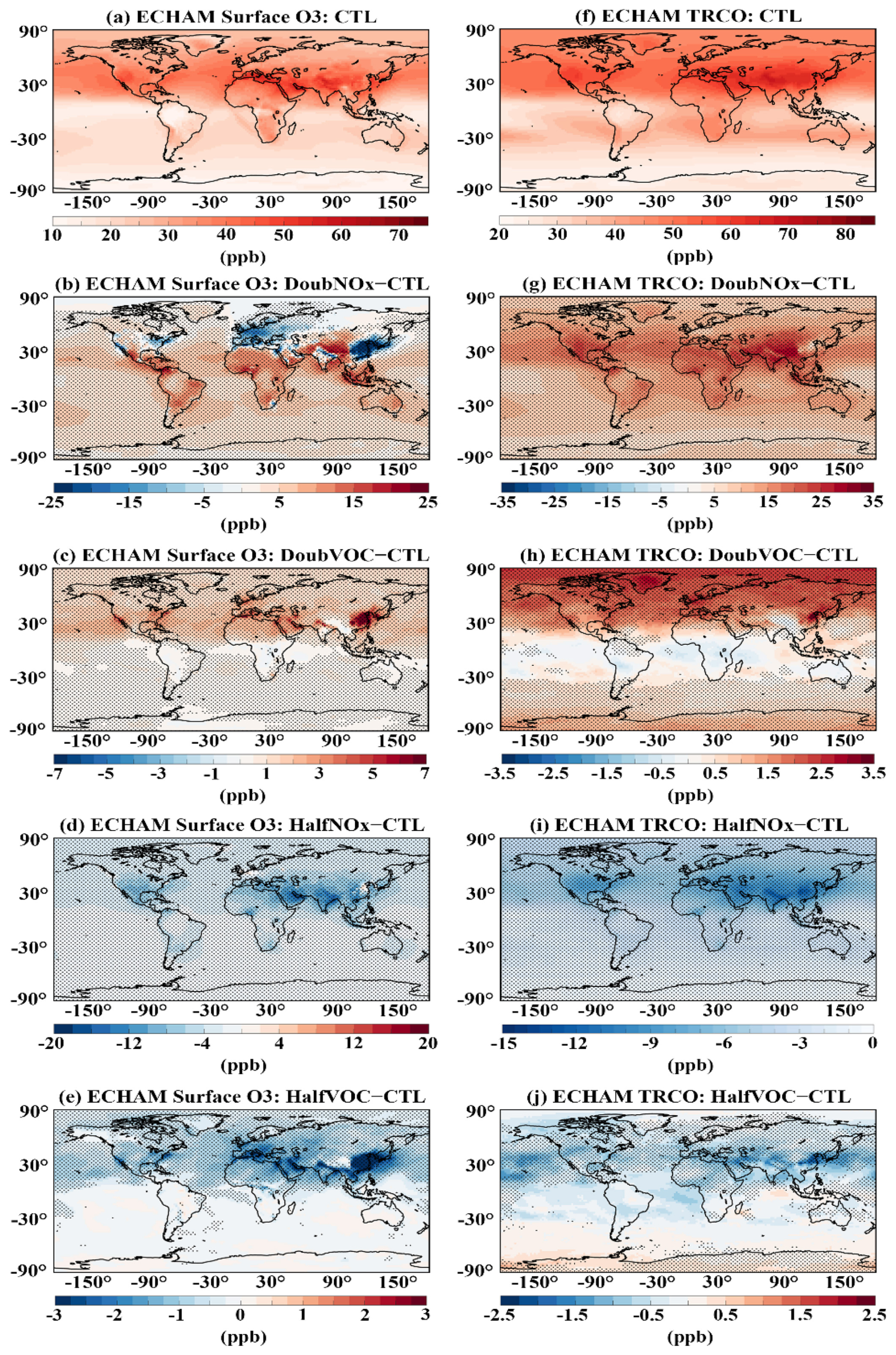
Figure 3 Spatial distribution of surface ozone (ppb) for (a) from CTL simulations. Anomalies from (b) DoubNO_x – CTL, (c) DoubVOC – CTL, (d) HalfNO_x – CTL and (e) HalfVOC – CTL simulations. Panels (f)–(j) are the same as (a)–(e) but for TRCO. The stippled regions in the figures indicate anomalies significant at 95 % confidence based on the t test.

Further, we show the impact of emission changes on the TRCO distribution (Fig. 3f–j). The estimated global mean TRCO from the CTL simulation from 1998 to 2019 is 39.4 [23.8 to 56.8] ppb (Fig. 3f). CTL simulations show higher amounts of TRCO (40.9 to 68.8 ppb) in the latitudinal band of 20 to 40° N. These concentrations are pronounced over South and East Asia, spanning from the Mediterranean region to eastern China (Fig. 3f). TRCO anomalies from DoubNO_x – CTL show enhancement by 11.7 [6.9 to 19.8] ppb (global mean) (Fig. 3g). In the 20–40° N belt, the TRCO anomalies increase by 6.1–29.3 ppb, particularly over South Asia. Interestingly, in highly urbanised areas such as the IGP, Southeast China, Northeast US and Europe, there is only a marginal increase in TRCO anomalies (∼ 5 ppb). This suggests the existence of a distinct ozone photochemical regime in these regions. Further exploration of this aspect is discussed in Sects. 4 to 6.

The impact of the doubling of VOC emissions (anomalies from DoubVOC – CTL simulations) on TRCO is depicted in Fig. 3h. An increase in global mean TRCO by 1 [−0.2 to 2.4] ppb is observed in this emission scenario. It should be noted that TRCO anomalies from DoubVOC – CTL are 10 times less than that from DoubNO_x – CTL (Fig. 3g and h). Large values of TRCO anomalies (1.5–2) are observed in the high latitudes (north of 60° N) and South and East Asia, with the largest values of more than 2.5 ppb over East China (e.g. Beijing). Interestingly, slight decreases in TRCO are seen in the tropical regions. This is consistent with the recent finding that aromatics, especially benzene, can lead to efficient ozone destruction in tropical UTLS (Rosanka et al., 2021). The TRCO anomalies in response to the reduction in NO_x emission by 50 % (HalfNO_x – CTL) show negative TRCO anomalies all over the globe (Fig. 3i). The global mean TRCO anomalies are reduced by −3.7 [−7.9 to −1.1] ppb. Large decreases in TRCO anomalies are seen over Arabia and South and East Asian regions (2.6–12.8 ppb). The TRCO anomalies from HalfVOC – CTL show an overall decrease in TRCO by −0.27 [−0.97 to −0.4] ppb (Fig. 3j). Further, a small enhancement is noted in the TRCO anomalies (by 0.5–1 ppb) in the southern tropics and south polar region, while a decrease of −2.3 to 0.3 ppb is observed in the NH. (Fig. 3j). Figure 3 clearly portrays that the TRCO response to NO_x emission change is larger than that of VOCs. There is a spatially distinct distribution in TRCO associated with the region-specific ozone photochemical regimes (more discussion on the ozone photochemical regimes is detailed in Sects. 4–6).

3.3 Spatial distribution of trends in ozone

We estimate trends in TRCO from ECHAM CTL simulations (1998–2019) and OMI/MLS satellite retrievals (2005–2019). The simulated trends are compared with satellite retrieves for the period 2005–2019. Since IASI-GOME2 has a short observation period (2017–2019) and IASI-SOFRID has negative drift in the SH, only TRCO from OMI/MLS is considered for trend estimation (Fig. 4). The spatial pattern of trends from OMI/MLS shows fair agreement with model simulations (Fig. 4a–b). Quantitatively, the global mean TRCO trend from OMI/MLS is slightly lower than the model (OMI/MLS: 1.43 [−0.5 to 3.2] ppb decade⁻¹; ECHAM CTL: 1.58 [0.3 to 3.3] ppb decade⁻¹). Both datasets reveal high trends, ranging from 3–4 ppb decade⁻¹ across regions such as South Asia, East Asia and the West Pacific. OMI/MLS show negative trends over parts of Africa; South America; Australia; and the southeastern Pacific (Fig. 4b), which is not simulated in ECHAM6–HAMMOZ. Although there is fair agreement in spatial patterns of TRCO trends between OMI/MLS and the model, the minor differences may be due to the model's tendency to underestimate ozone levels and differences in the seasonal cycle (see Fig. 1).

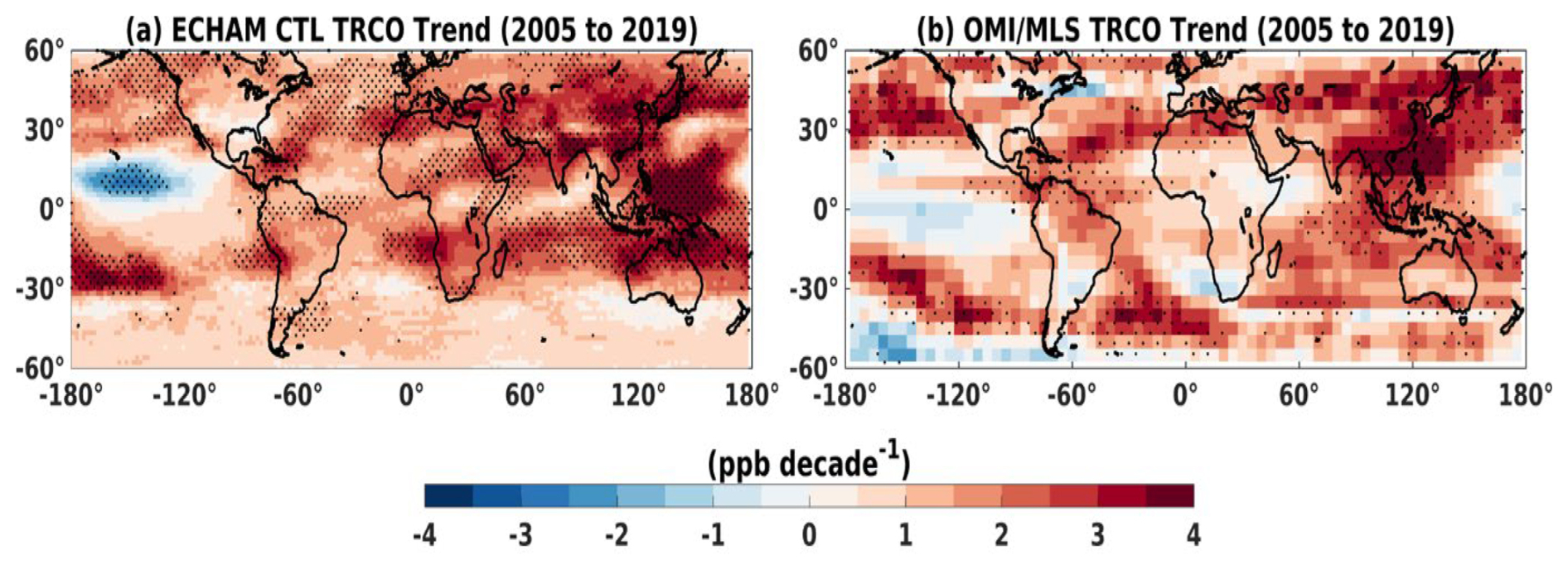
Figure 4 Trend of TRCO (ppb decade⁻¹) from (a) ECHAM CTL and (b) OMI/MLS satellites for the period from January 2005 to December 2020. Stippled regions in the figures indicate trends significant at the 95 % confidence level based on the t test.

TRCO trends analysed from the Total Ozone Mapping Spectrometer (TOMS) indicate a consistent absence of a trend over the tropical Pacific Ocean, with notable positive trends (4 %–5 % decade⁻¹) seen in the mid-latitude Pacific regions of both hemispheres (Ziemke et al., 2005). This pattern is consistent across the ECHAM6–HAMMOZ and OMI/MLS data, although their magnitude differs (Fig. 4a–b). TOMS data also showed trends of ∼ 2 %–5 % decade⁻¹ across broad regions of the tropical South Atlantic, India, Southeast Asia, Indonesia and the tropical/subtropical regions of China during 1979–2003 (Ziemke et al., 2005; Beig and Singh, 2007) which are also simulated in the model. Further, a large positive trend of ∼ 2.5 ppb decade⁻¹ observed near 50° S in OMI/MLS is not simulated by the model (Fig. 4a–b). The CESM2–WACCAM6 simulation from 1950 to 2014 also shows the largest trend estimate of 0.8 Tg decade⁻¹ over 20–30° N (Fiore et al., 2022). Large TRCO trends over 20–30° N are also seen in OMI/MLS and the model (Fig. 4). Wang et al. (2021) reported TRCO trends varying between 2.55 and 5.53 ppb decade⁻¹ during 1995–2017 over South and East Asia using IAGOS, ozonesonde observations and Goddard Earth Observing System – chemistry model (GEOS-Chem). Our model also shows similar increasing trends.

Figure 5 shows the spatial distribution of estimated trends in surface ozone and TRCO from CTL simulation for the period 1998–2019. Changes (doubling/halving) in the emission of NO_x and VOCs will change ozone trends. Hence, we also analysed anomalies in ozone from DoubNO_x – CTL, DoubVOC – CTL, HalfNO_x – CTL and HalfVOC – CTL. The surface ozone trend in the CTL simulation shows spatial variation with a pronounced increasing trend over South Asia and the Middle East (3–4 ppb decade⁻¹) (Fig. 5a). A similar pronounced increase is also seen in the TRCO trend (Fig. 5b). The estimated global mean TRCO trend from CTL is 0.89 [−0.07 to 2.1] ppb decade⁻¹. However, the negative trends in surface ozone over Mexico, certain parts of the US and East China are barely discernible in the TRCO data. This discrepancy may stem from the interplay of mixing and transport processes and stratospheric intrusions, which are crucial when assessing ozone levels across the tropospheric column. The stratospheric ozone intrusions lead to an enhancement in the tropospheric ozone (Prather and Zhu, 2024).

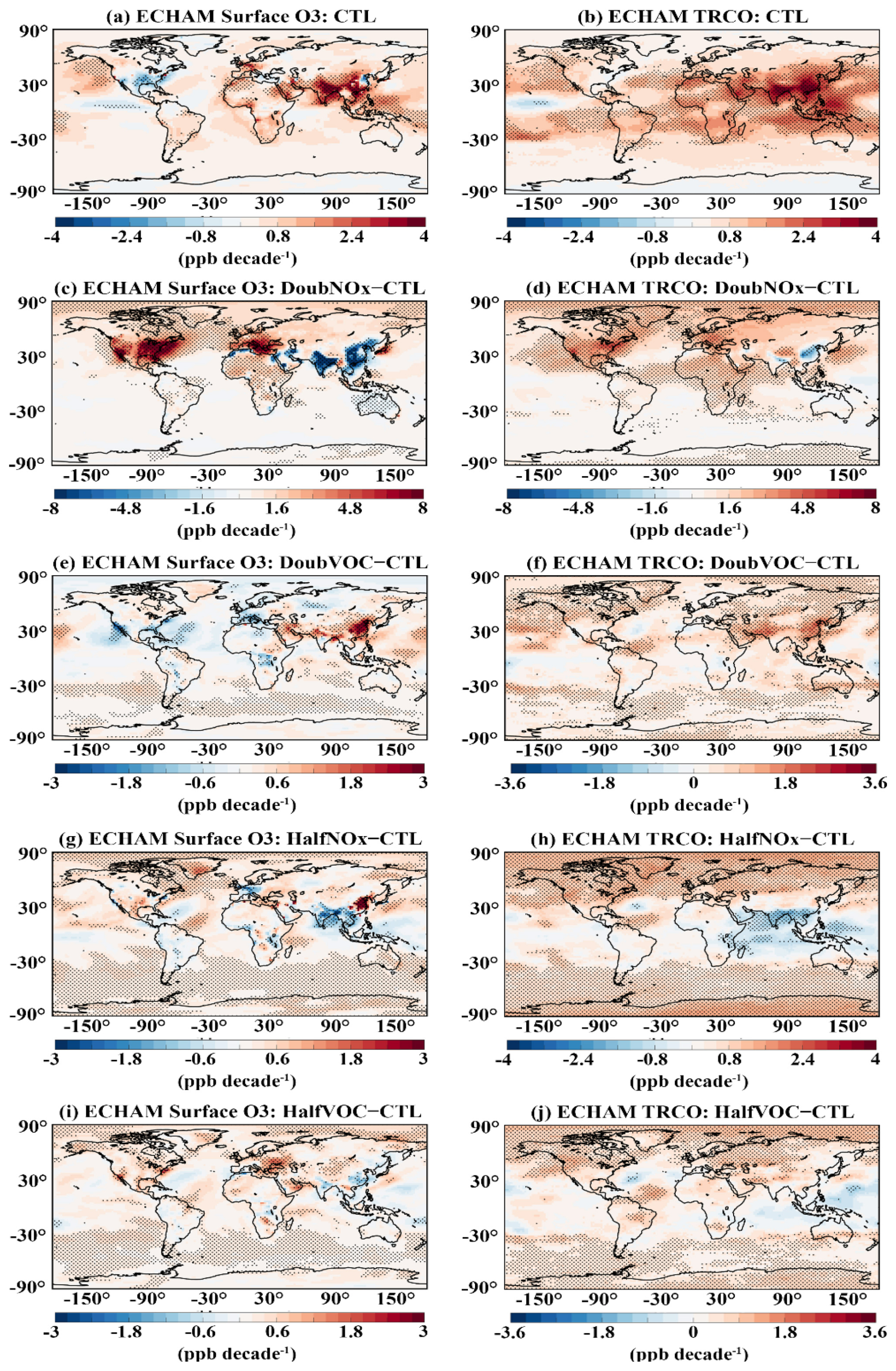
Figure 5 Trend in surface ozone (ppb decade⁻¹) for the period from 1998–2019 calculated from (a) CTL and ozone anomalies in (c) DoubNO_x – CTL, (e) DoubVOC – CTL, (g) HalfNO_x – CTL and (i) HalfVOC – CTL simulations. Panels (b), (d), (f), (h) and (i) represent the corresponding trend in TRCO. The stippled regions in the figures indicate significance at the 95 % confidence level based on the t test.

Figure 5c–d show the trend in surface ozone and TRCO estimated from anomalies obtained from DoubNO_x – CTL simulations. A striking feature is the large negative trend over India and China at the surface (−4.8 to −8 ppb decade⁻¹) and TRCO (−2 to −4 ppb decade⁻¹), whereas Europe, the US, some parts of Africa and South America show positive trends at the surface (1.8 to 8 ppb decade⁻¹) and TRCO (2 to 4 8 ppb decade⁻¹). The global mean TRCO trend is 1.2 [−0.1 to 2.7] ppb decade⁻¹.

When global emissions of VOCs are doubled, the trend in ozone estimated from anomalies (DoubVOC – CTL) shows a decrease (by −0.8 to −1.9 ppb decade⁻¹) in surface ozone over Europe, Africa and some parts of the US, while a strong positive trend (1.6 to 2 ppb decade⁻¹) is seen over India and China (Fig. 5e). TRCO trends show an enhancement over South Asia, Southwest Asia, China, parts of the Indian Ocean and the western Pacific (0.8 to 1.6 ppb decade⁻¹) (Fig. 5f). The global mean TRCO trend for the DoubVOC – CTL simulation is 0.5 [−0.03 to 1.04] ppb decade⁻¹. The estimated enhancement in global mean TRCO trend for DoubVOC is less than for DoubNO_x simulations. Figure 5c and e also give indications of the existence of distinct ozone photochemical regimes globally. The increasing (decreasing) trend in surface ozone with an increase in VOC (NO_x) over India and China indicates that these regions are in a VOC-limited regime, and vice versa, over the US and Europe indicates that these regions are in a NO_x-limited regime (more discussions in Sects. 4 to 6).

Figure 5g–h show the trend in surface and TRCO ozone estimated from anomalies from HalfNO_x – CTL. The surface ozone trend shows a large negative trend over Europe and South Asia, while there is a positive trend over the US, China and Australia (Fig. 5g). Trends in TRCO also show a large negative trend over South Asia (Fig. 5h). Although anthropogenic NO_x emissions are halved compared to CTL, ozone trends are positive over large regions globally. Our investigations reveal that the trend in VOC anomalies from the HalfNO_x – CTL simulations is positive over the US, India and Europe, while it is negative over China. Similarly, the trend in NO_x anomalies from the HalfNO_x – CTL simulations is positive over the US and Europe, while it is negative over India and China (Fig. S1a–b). It should be noted that over the US and Europe, the positive NO_x trend estimated from anomalies (HalfNO_x – CTL) suggests that NO_x levels in HalfNO_x are declining more slowly compared to CTL, leading to relatively higher NO_x concentrations over time. Meanwhile, over India and China, the NO_x level is weak in HalfNO_x compared to CTL, leading to a negative trend estimated from NO_x anomalies (HalfNO_x – CTL).

It is known that the ozone response is nonlinear to NO_x and VOC emission changes and depends on the local photochemical regime. In the US, estimated trends from anomalies are positive in VOC and NO_x (HalfNO_x – CTL). This indicates that relatively more ozone precursors in the HalfNO_x contribute to the observed positive ozone trend. Over Europe, the strong positive trend estimated from NO_x anomalies (compared to VOCs) enhances NO_x titration effects, contributing to the observed negative ozone trend. China, being a VOC-limited regime, experiences reduced NO_x titration under lower-NO_x conditions, resulting in positive ozone trends. Over India, the positive trend in VOC anomalies with a negative trend in NO_x anomalies may enhance the radical destruction of ozone caused by aromatic hydrocarbons in low-NO_x conditions (Taraborrelli et al., 2021), resulting in a negative ozone trend. For HalfNO_x – CTL, the global mean trend is positive at 0.47 [−0.76 to 1.3] ppb decade⁻¹.

The trend in surface and TRCO ozone estimated from anomalies from HalfVOC – CTL is shown in Fig. 5i–j. A large negative trend in surface ozone is noted over IGP and China, while an insignificant positive trend is noted over the US and Europe (Fig. 5i). The TRCO trend is positive over large regions in the world with pronounced high values over the mid-latitudes and high latitudes although emissions of all anthropogenic VOCs are halved (Fig. 5j). The global mean trend for HalfVOC – CTL is 0.37 [−0.35 to 1.02] ppb decade⁻¹. Our analysis shows that the trend in NO_x anomalies and VOC anomalies from HalfVOC – CTL is decreasing over both India and China (Fig. S1c–d). The negative trend in precursors might have resulted in a negative trend in ozone over these regions. The absence of strong trends in TRCO (Fig. 5b, d, f, h, j) similar to that at the surface (Fig. 5a, c, e, g, i) in all the simulations indicates the potential contribution of transport in the troposphere and stratospheric intrusions in TRCO. Ozone injection through stratosphere–troposphere exchange is an important source of tropospheric ozone (Prather and Zhu, 2024).

3.4 Trends in emission and tropospheric column of NO₂ and HCHO

We show mean emissions of NO_x (NO + NO₂) and HCHO over urban/semi-urban regions, US, Brazil, Europe, Africa, India, China and Australia, in Fig. 6. High emissions of VOCs and NO_x in India and China are evident in Fig. 6. Furthermore, VOC emissions are noted to be higher than NO_x over all the regions. They are higher by a factor of 3.3 in the US, 11.3 in Brazil, 4.8 in Europe, 10.5 in Africa, 10.8 in India, 6.1 in China and 6.7 in Australia.

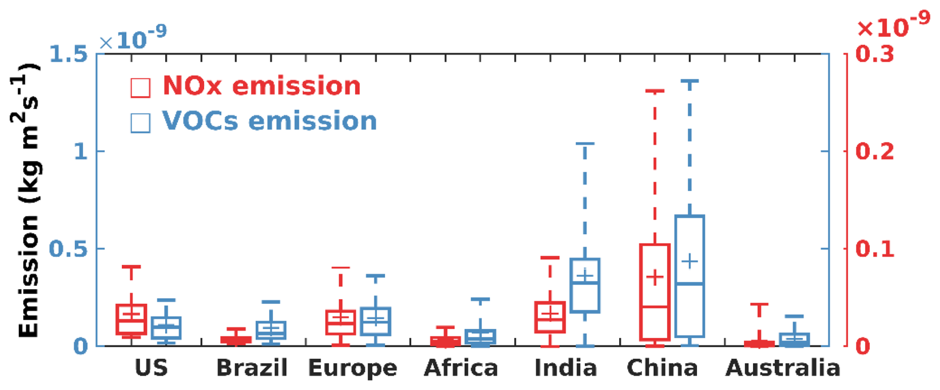
Figure 6 Box-and-whisker plot illustrating the NO_x (NO + NO₂) and VOCs emission over the regions US (85–110° W, 35–44° N), Brazil (34–49° W, 24–3° S), European Union (9° W–45° E, 35–55° N), central Africa (14° W–45° E, 0–14° N), India (75–90° E, 8–30° N), China (110–125° E, 30–42° N) and South Australia (134–154° E, 38–28° S) from the ECHAM model. The box represents the 25th and 75th percentiles, and the whisker represents the 5th and 95th percentiles. The plus marker represents the mean, and the horizontal bar represents the 1st and 99th percentiles.

The trends in ozone are partly modulated by the change in the emission of its precursors and partly by meteorology (e.g. Verstraeten et al., 2015). We show trends in emissions and tropospheric column amounts of ozone precursors NO₂ and HCHO from ECHAM CTL and OMI satellite retrievals in Fig. 7. NO₂ and HCHO are considered here because column densities of these is used to identify the ozone photochemical regimes discussed in Sects. 4–6. Emissions and tropospheric columns of HCHO and NO₂ from ECHAM CTL show large positive trends over the South and East Asian regions (Fig. 7a–d). These regions show large positive ozone trends in both model and OMI satellite data (see Figs. 4 and 5). Over Europe and the US, the emission trend in both HCHO and NO₂ from the model is negative (Fig. 7a, c). Though a similar negative trend in tropospheric column NO₂ is seen over these regions, a marginal positive trend is noted for HCHO (Fig. 7b, d). The positive trend in column HCHO could be due to secondary production pathways from biogenic emissions or methane oxidation and transport (e.g. Anderson et al., 2017; Alvarado et al., 2020). The positive trend in ozone (Figs. 4a, b and 5a, f) along with a negative trend in NO₂ and HCHO (Fig. 7a–d) over Europe indicates that ozone production over this region has been initially controlled by VOCs (i.e. VOC-limited regime; detailed discussed in Sect. 4). However, a large decreasing trend in NO₂ compared to that of HCHO over this region might have decreased the NO_x titration effect, resulting in an increase in ozone. On the contrary, a negative trend in surface ozone (Fig. 5a), along with negative trends in NO₂ and HCHO, is seen over the US (Fig. 7a–b). The decrease in both NO₂ and HCHO would have resulted in a decreasing trend in surface ozone over this region. This also indicates that the US might have been in a NO_x-sensitive regime before and the large negative trend in NO₂ might have resulted in the decreasing trend in ozone (discussed further in Sects. 4–6).

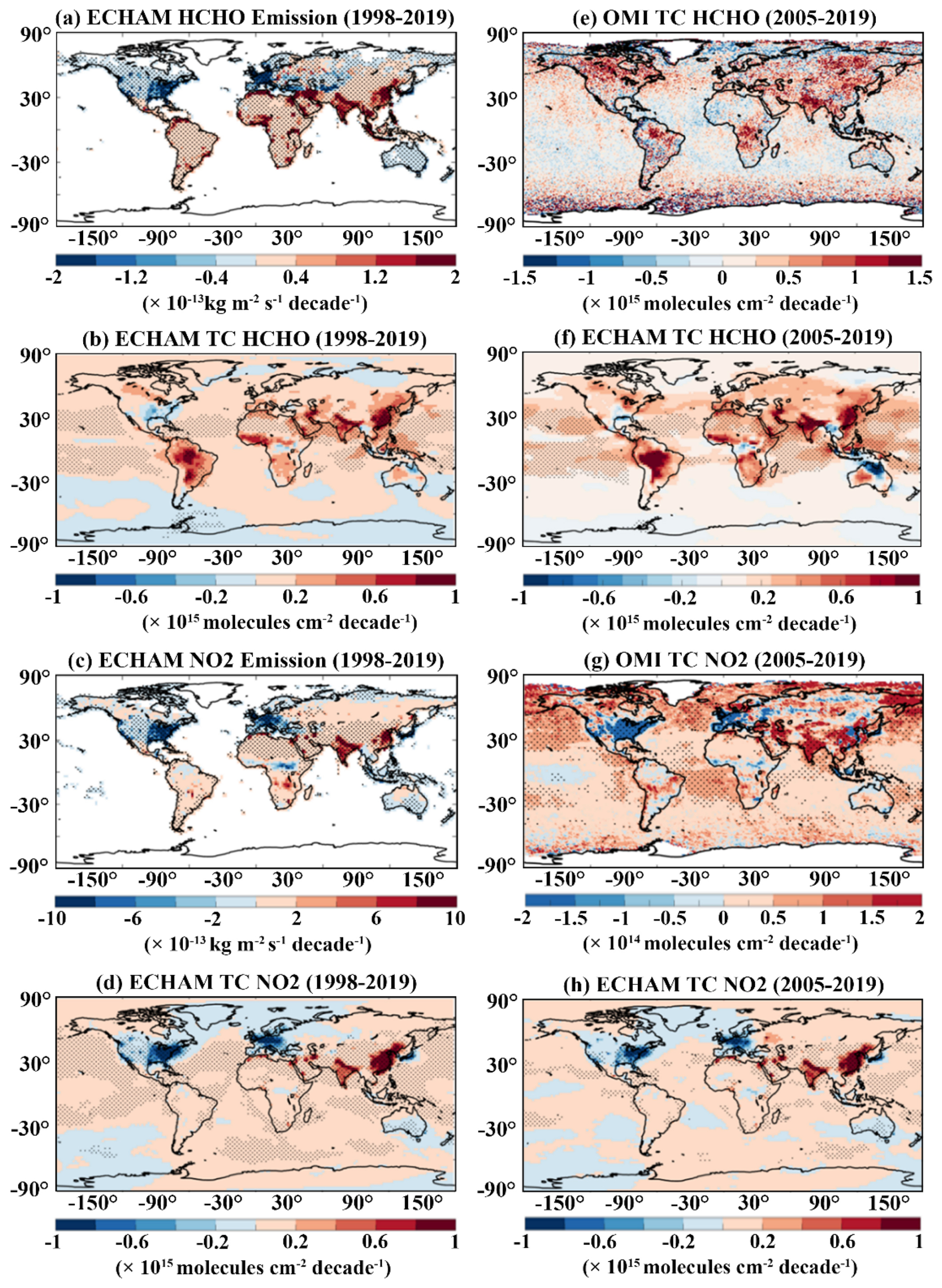
Figure 7 Trend in anthropogenic emission (kg m² s⁻¹ decade⁻¹) from ECHAM CTL simulation for the period 1998–2019 for (a–b) HCHO and NO₂, respectively. Trends in tropospheric column (TC) (molec. cm⁻² decade⁻¹) for (c–d) HCHO and NO₂, respectively. The trend in tropospheric column of HCHO from (e) OMI and (f) ECHAM CTL simulations for the period from 2005–2019. (g)–(h) are the same as that of (e)–(f) but for tropospheric column NO₂. The stippled regions in the figures indicate significance at the 95 % confidence level based on the t test.

Further, we compared the simulated trends in column HCHO and NO₂ with the OMI retrievals for the period 2005–2019 (Fig. 7e–h). OMI shows a positive trend in tropospheric column HCHO over South Asia (1–1.5 × 10¹⁵ molec. cm⁻² decade⁻¹), parts of western China (0.75–1.25 × 10¹⁵ molec. cm⁻² decade⁻¹), the Iranian Plateau (0.5–1 × 10¹⁵ molec. cm⁻² decade⁻¹), the Amazon (1–1.5 × 10¹⁵ molec. cm⁻² decade⁻¹), North America (0.5–1.5 × 10¹⁵ molec. cm⁻² decade⁻¹), Europe (0.5–1 × 10¹⁵ molec. cm⁻² decade⁻¹) and central Africa (1–1.5 × 10¹⁵ molec. cm⁻² decade⁻¹). The model simulated trends show reasonable agreement with OMI, except for western areas in central Africa, north Africa, southwest and southeast China, and some parts of Australia. Over these regions, OMI indicates a negative trend, while the model suggests a marginal positive trend. OMI and ECHAM CTL show a good agreement in the tropospheric column NO₂ trend. Both datasets show negative trends over the eastern US and Europe and positive trends over the Middle East and South Asia. However, differences are seen in eastern China and central Africa, where OMI indicates a negative trend, while the model shows a strong positive trend. The differences between simulated and OMI HCHO and NO₂ column trends may be due to sampling time and differences in seasonal cycle. Figures 4, 5 and 7 clearly indicate the impact of ozone precursors on the spatial distribution of ozone trends. This warrants a detailed discussion on the spatial distribution of ozone precursors and their impact on ozone-production-sensitive regimes, which are presented in the next section.

4 Influence of NO_x and VOCs emissions on formaldehyde-to-nitrogen dioxide ratio

In this section, we diagnose the spatial distribution of tropospheric ozone production sensitivity regimes (NO_x-limited/VOC-limited) associated with simulations of emission changes using formaldehyde-to-nitrogen dioxide ratio (FNR). We estimate the FNR thresholds from ECHAM6–HAMMOZ model simulations adhering to the methodology outlined by Jin et al. (2017). The procedure to obtain FNR threshold from monthly mean data involves two steps: (1) obtaining the ozone response from emission sensitivity simulations (here, HalfNO_x and HalfVOC simulations) by considering only the polluted cells over the study region and plotting it as a function of FNR (Fig. 8a) and (2) calculating cumulative probability from these data for the conditions d$\left[{\mathrm{O}}_{\mathrm{3}}\right]/\mathrm{d}{E}_{{\mathrm{NO}}_x}<$ 0) (VOC-limited) and (d$\left[{\mathrm{O}}_{\mathrm{3}}\right]/\mathrm{d}{E}_{{\mathrm{NO}}_x}>$ d$\left[{\mathrm{O}}_{\mathrm{3}}\right]/\mathrm{d}{E}_{\mathrm{VOC}}$ > 0) (NO_x-limited) (Fig. 8b), where d[O${}_{\mathrm{3}}]/\mathrm{d}E$ represents the change in ozone corresponding to a change in emission of either NO_x or VOCs. This approach is applied to estimate FNR thresholds to distinctly delineate the ozone photochemical regimes as NO_x- or VOC-limited over major urban and semi-urban regions. The regions considered for estimating the FNR are shown in Fig. 9.

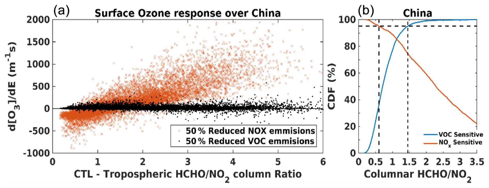
Figure 8 (a) Typical example of a normalised surface ozone sensitivity to a 50 % reduction in global NO_x (HalfNO_x) and VOC (HalfVOC) emissions versus the tropospheric column HCHO $/$ NO₂ ratio derived from ECHAM6–HAMMOZ model simulation over China for the period from 1998–2019. (b) Cumulative probability (CP) of VOC-sensitive (d$\left[{\mathrm{O}}_{\mathrm{3}}\right]/\mathrm{d}{E}_{{\mathrm{NO}}_x}<\mathrm{0}$) and NO_x-sensitive (d$\left[{\mathrm{O}}_{\mathrm{3}}\right]/\mathrm{d}{E}_{{\mathrm{NO}}_x}>$ d$\left[{\mathrm{O}}_{\mathrm{3}}\right]/\mathrm{d}{E}_{\mathrm{VOC}}>$ 0) conditions as a function of tropospheric column HCHO $/$ NO₂ and simulated by the ECHAM6–HAMMOZ model. The horizontal dashed line represents the 95 % CP, and the vertical dashed lines represent the HCHO $/$ NO₂ ratio corresponding to 95 % CP for both the VOC-sensitive and NO_x-sensitive curves demarcating the VOC-sensitive, NO_x-sensitive and transition regimes.

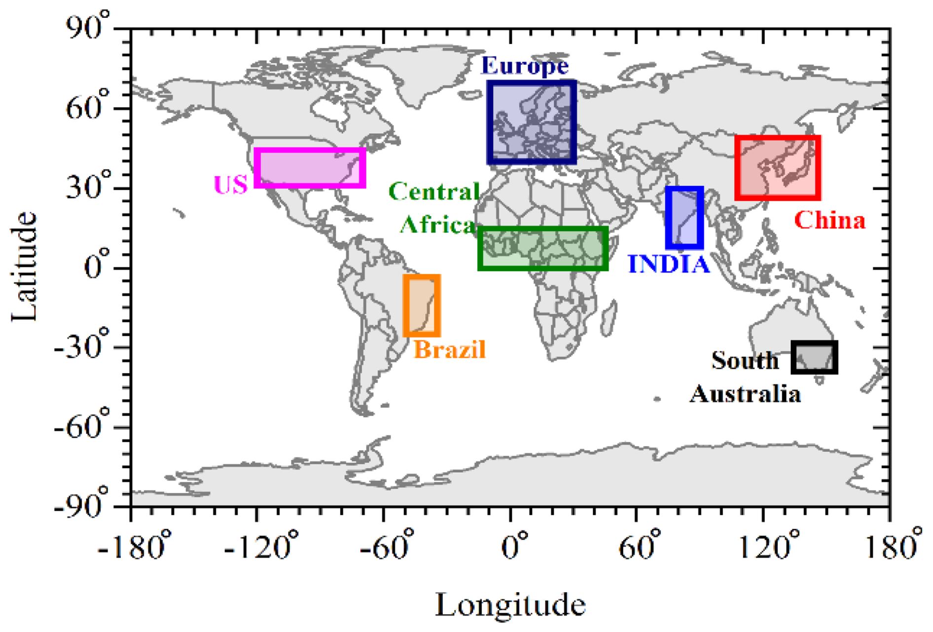
Figure 9 The rectangular box marks indicate the regions considered for estimating the HCHO $/$ NO₂ ratio (FNR).

Further, we compared the model-estimated FNR with the OMI-derived FNR for the period 2005–2019. Figure 10 illustrates the comparison of FNR estimated from ECHAM6–HAMMOZ CTL simulations with OMI. The spatial map of FNR shows fairly good agreement between OMI and the model. Over the urbanised regions (e.g. South Asia, Europe, the US and China), both the model and OMI show FNR < 4. In contrast, regions like North Canada, South America, central Africa, Australia and Siberia exhibit high FNR values > 9. There is good agreement between the model simulations and OMI; however, some minor differences are seen between the model and OMI FNR over the west coast of South America, South Africa, the Tibetan Plateau and western Australia.

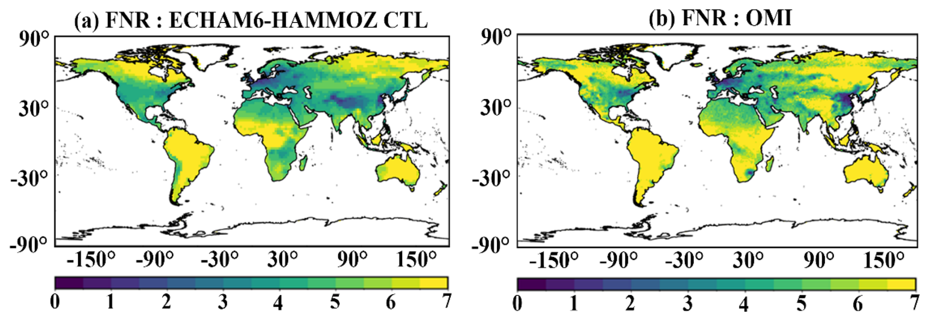
Figure 10 Spatial distribution of mean tropospheric column HCHO $/$ NO₂ (FNR) obtained from ECHAM6–HAMMOZ CTL simulations (2005–2019) and OMI (2005–2019).

These differences could be due to the underestimation of HCHO in the model over these regions. Considering the fair performance of the model in comparison with OMI, we further analysed the influence of changes in NO_x and VOC emissions on the FNR from the model simulations, which are discussed in the subsequent sections.

Since the emission of HCHO and NO₂ varies with the seasons across the globe (e.g. De Smedt et al., 2015; Wang et al., 2017; Surl et al., 2018; Kumar et al., 2020; Goldberg et al., 2021; Guan et al., 2021), understanding the seasonal changes in FNR is crucial for comprehending shifts in ozone photochemical regimes. In this regard, we extracted the seasonal changes in transition limits for the major urban and semi-urban regions shown in Fig. 9 and summarised in Table 1. Figure 11 illustrates the seasonal variation in estimated FNR from both OMI data and model simulations across these key urban regions. In general, all regions exhibit distinct seasonal variations in transition limits (Table 1). Previously reported transition limits over the US (2–5: Johnson et al., 2024; 1.1–4: Schroeder et al., 2017) and China (0.6–1.5/1.25–2.39; Chen et al., 2023) during the summer season are also compared with our model estimates. The estimated FNR values from the ECHAM6–HAMMOZ simulations show fair agreement over both locations (0.4–4.6 in the US and 0.58–2.56 in China) with some minor differences. These minor discrepancies in the estimated FNR could be due to differences in the chosen location, time period and dataset used. Chen et al. (2023) have also reported that the transition limits depend on the region considered for the analysis.

Based on the threshold values depicted in Table 1 and the mean FNR in Fig. 11, the seasonal change in ozone photochemical regimes over the key regions associated with the different emission scenarios are assessed. In the CTL simulation (Fig. 11e–h), the US, Europe and China are found to be in the transition regime, while all other regions are NO_x-limited during winter. In spring, every region except India remains NO_x-limited, with India transitioning into the transition regime. During summer and autumn, all regions shift to a NO_x-limited condition. We further compared the model-estimated regional FNR from the CTL simulation with the OMI-derived FNR shown in Fig. 11a–d. The ozone photochemical regimes inferred from both OMI and the model show consistent results except during winter. During winter, the US, Europe and China are NO_x-limited in OMI, while our model shows them in the transition regimes.

Doubling NO_x (DoubNO_x) leads to a shift to a VOC-limited regime in all regions except Africa and Australia during winter, spring and autumn (Fig. 11i–l). The relatively high VOC contributions in Africa and Australia likely keep these regions in the transition regime. During summer, the US, Europe, Africa and Australia transform to the transition regimes, while all other regions remain VOC-limited. In both the DoubVOC and HalfNO_x scenarios (Fig. 11m–t), ozone photochemical regimes show no seasonality. All regions consistently exhibit a NO_x-limited regime throughout all seasons. In the HalfVOC simulation (Fig. 11u–x), the US, Europe and China are in transition regimes, while all other regions become NO_x-limited during winter. India remains in a transition regime during all other seasons, whereas other regions consistently exhibit NO_x-limited conditions. Figure 11 also depicts that DoubNO_x and HalfNO_x simulations greatly impact the shift in ozone photochemical regimes compared with DoubVOC and HalfVOC simulations. This indicates that ozone photochemistry is highly sensitive to changes in NO_x emissions globally.

Table 1 Seasonal mean estimated values of the tropospheric HCHO $/$ NO₂ columns threshold ratios from ECHAM6–HAMMOZ model control simulation to identify the NO_x and VOC sensitive regimes across regions mentioned in Fig. 9. The FNR less than the lower limit indicates VOC-limited and that higher than the upper limit indicates NO_x-limited regimes.

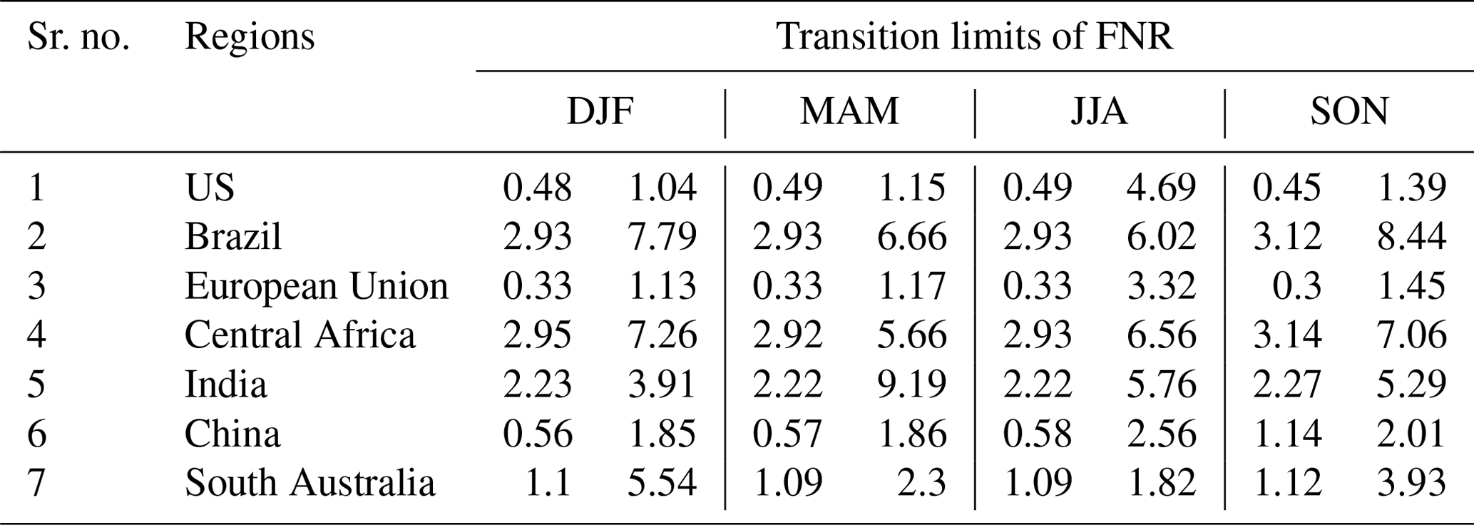
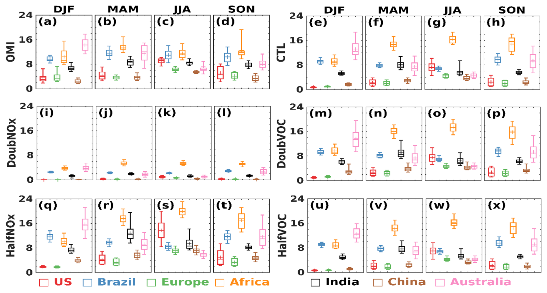
Figure 11 Box-and-whisker plot illustrating the long-term seasonal average FNR over the regions depicted in Fig. 7 from (a–d) OMI observations and model (e–h) CTL, (i–l) DoubNO_x, (m–p) DoubVOC, (q–t) HalfNO_x and (u–x) HalfVOC simulations. The box represents 25th and 75th percentiles and the whisker represents the 5th and 95th percentiles. The plus marker represents the mean, and the horizontal bar represents the 1st and 99th percentiles.

5 Influence of NO_x and VOCs emissions on trends of formaldehyde-to-nitrogen dioxide ratio

Trend analysis is carried out on FNR to understand the temporal evolution of ozone photochemical regimes associated with different emission scenarios. Figure 12 illustrates trends of FNR during the period 1998–2019 from CTL, DoubNO_x, DoubVOC, HalfNO_x and HalfVOC simulations. In the CTL simulation, decreasing (negative) trends in FNR are seen over the Asian region (−0.4 to −1.2 decade⁻¹) and Australia (−0.8 to −1.6 decade⁻¹), and an increasing (positive) trend is seen in Europe (0.2 decade⁻¹) and the US (0.8–1.4 decade⁻¹) (Fig. 12a). These observed trends in FNR are mainly driven by the region-specific trends in HCHO and NO₂ (Fig. 7). Figure 7 shows a higher positive trend in NO₂ than in HCHO in the Asia region, causing an overall decreasing trend in FNR and indicating a tendency toward VOC-limited regimes, whereas, over the US and Europe, there is a higher negative trend in NO₂ than HCHO, causing a positive trend in FNR, indicating a tendency toward a NO_x-limited regime. A recent study by Elshorbany et al. (2024) also reported a significant positive trend over Europe and the US and a negative trend over Asia using the OMI-based tropospheric column HCHO $/$ NO₂ ratio. Further, long-term column measurements of HCHO and NO₂ from OMI over India and China have revealed an increasing trend in NO₂ compared to that of HCHO, causing a decreasing trend in FNR over these regions (Jin and Holloway, 2015; Mahajan et al., 2015).

The DoubNO_x simulation (Fig. 12b) shows a similar spatial trend pattern to that of CTL simulation (Fig. 12a). However, the magnitude of this trend is less than that of the CTL. For example, a weak positive trend is noted in the US and Europe (0.2–0.4 decade⁻¹), while trends over India and China are less negative (−0.2 to −0.4 decade⁻¹) in DoubNO_x than CTL (Fig. 12b). On the contrary, the magnitude of the positive trend over Canada and the negative trend over central Africa increased in DoubNO_x emission, while the negative trend over Australia became nominal and insignificant. This indicates that Canada and central Africa have a tendency to become NO_x-limited and VOC-limited, respectively.

In DoubVOC simulations, trends are marginally increasing over the US, Canada and Europe compared to the CTL (Fig. 12a and c). A notable change is observed over the Middle East and Amazon, where trends become more negative and positive, respectively, compared to CTL. The negative trends over Australia in the CTL become nominal and insignificant in the DoubVOC simulation. In HalfNO_x simulations (Fig. 12d), the positive trends are higher over the US, Europe and Amazon, while negative trends prevail over India, China and northeast Australia. Meanwhile, in HalfVOC simulations, marginal changes are noted globally compared to CTL. The most pronounced change in the FNR trend is observed over West Australia, where the negative trend in CTL becomes positive in HalfVOC (Fig. 12e). Figure 12f clearly shows that the trend in FNR is always negative over India and China for all the simulations, indicating that these regions have a tendency to become VOC-limited, while the positive trends over Europe and US show a tendency to become more NO_x-limited. Further, from Figs. 5, 11 and 12, we can infer that the relation between trends in FNR and ozone exhibits a nonlinearity. For example, even though FNR shows a negative trend over India and China for all the simulations, the TRCO trend depends on the specific emission scenario.

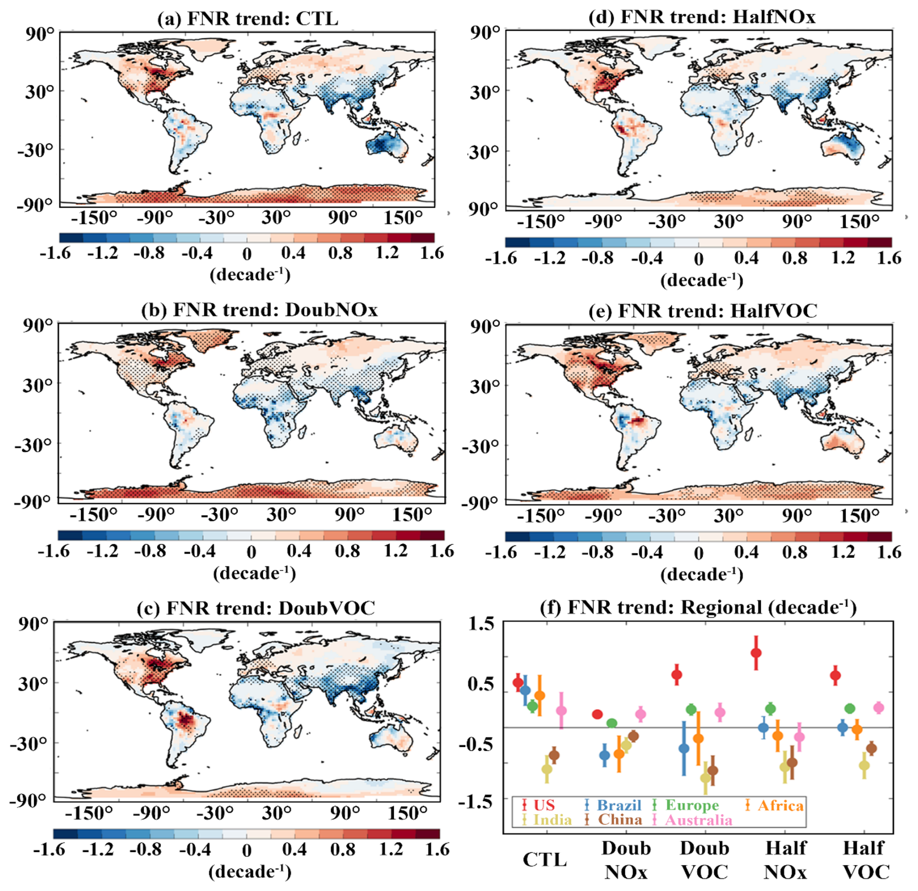
Figure 12 Trends in the tropospheric column HCHO $/$ NO₂ ratio during 1998–2019 from ECHAM6–HAMMOZ simulations for (a) for CTL, (b) DoubNO_x, (c) DoubVOC, (d) HalfNO_x and (e) HalfVOC simulations. The stippled region indicates the trend significant at 95 % confidence based on the t test. (f) Scatter plot illustrating the long-term trend and standard deviation over the regions depicted in Fig. 9.

6 Tropospheric ozone radiative effects

The impact of emission changes on the tropospheric ozone radiative effect (TO3RE) is estimated using the ECHAM6 model output and a radiative kernel method (see data and model experiments). The estimated TO3RE for different model simulations is shown in Fig. 13. In the CTL simulations (Fig. 13a), the estimated global mean area-weighted average TO3RE for the period 1998 to 2019 is 1.21 [1.1 to 1.3] W m⁻². High TO3RE is noted over North Africa and the Middle East region in NH (∼ 2.2 W m⁻²), while in SH, it is over Australia and South Africa (∼ 1.2 W m⁻²). TO3RE estimates from TES measurements (2005–2009) also show a peak of 1.0 W m⁻² in northern Africa, the Mediterranean and the Middle East in June, July and August (Bowman et al., 2013). Recently, Pope et al. (2024) reported TO3RE estimates from IASI-SOFID, IASI-FORLI and IASI-IMS for the period from 2008–2017. The values reported by Pope et al. (2024) are comparable with our CTL simulation (e.g. IASI-FORLI: 1.23 W m⁻², IASI-SOFRID: 1.21 W m⁻², IASI-IMS: 1.21 W m⁻² and ECHAM6: 1.22 W m⁻²).

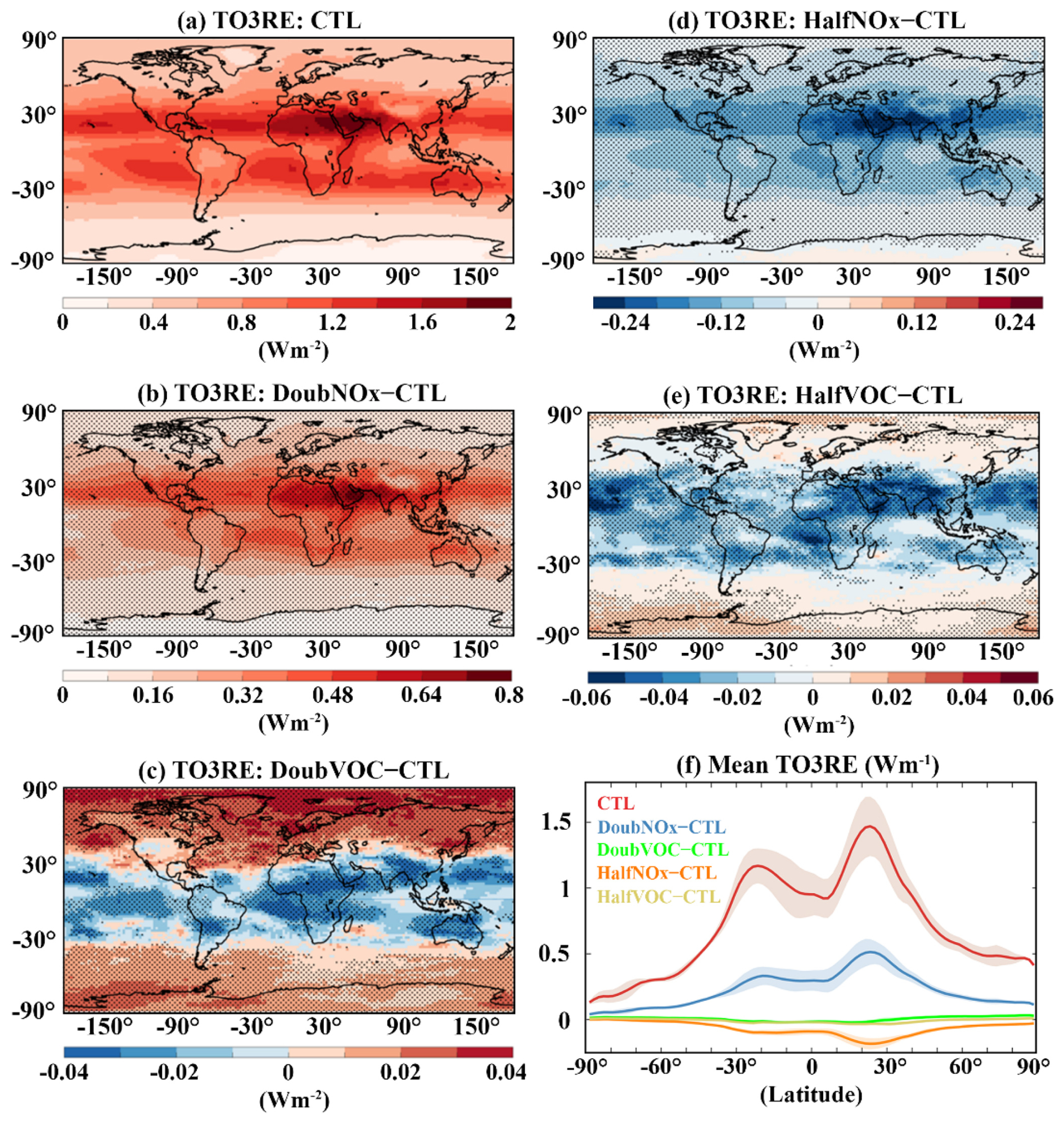
Figure 13 Tropospheric ozone radiative effects (TO3RE) (W m⁻²) for (a) CTL and anomalies from (b) DoubNO_x – CTL, (c) DoubVOC – CTL, (d) HalfNO_x – CTL and (e) HalfVOC – CTL simulations. Stippled regions in (b)–(e) indicate TO3RE significant at the 95 % confidence level based on the t test. (f) Line plot for zonal mean TO3RE (W m⁻²) from CTL, DoubNO_x – CTL, DoubVOC – CTL, HalfNO_x – CTL and HalfVOC – CTL shades indicate standard deviation.

The anomalies of TO3RE from DoubNO_x – CTL simulations are shown in Fig. 13b. Doubling of NO_x emissions causes an enhancement in TO3RE by 0.36 [0.23 to 0.5] W m⁻² compared to the CTL simulation. It shows a peak over the Middle East and adjacent North Africa (0.7 W m⁻²). A similar peak over this region is also seen in the CTL simulation. Doubling of VOC emissions causes a marginal decrease in global mean TO3RE by −0.005 [−0.05 to 0.04] W m⁻². TRCO enhancement for doubling NO_x is also higher than doubling VOC (see Fig. 3). DoubVOC – CTL simulations (Fig. 13c) show a peak over the Arctic (0.02 W m⁻²). The TO3RE anomalies are negative between 30° N and 30° S. These negative anomalies in TO3RE between 30° S and 30° N (Fig. 13c) can be attributed to negative anomalies of TRCO (Fig. 3h).

The reduction in NO_x emission by 50 % reduced global mean TO3RE by −0.12 [−0.2 to −0.05] W m⁻² than CTL. The anomalies in TO3RE from HalfNO_x – CTL simulations (Fig. 13d) show negative anomalies all over the globe, with a strong decrease over the Middle East and adjacent North Africa (−0.25 W m⁻²). Figure 13b and d show that the effect of enhancement/reduction in NO_x emissions is high over the Middle East and adjacent North Africa. The reduction in VOC emission by 50 % reduced global mean TO3RE by −0.03 [−0.07 to 0.02] W m⁻² compared to CTL simulations (Fig. 13e). HalfVOC – CTL simulations show negative anomalies of TO3RE between 40° S and 40° N and positive anomalies of 0.015 W m⁻² (low confidence) over mid–high latitudes in NH and SH. From Fig. 13, it is interesting to note that the magnitude of TO3RE and its response to emission change is pronounced over the Middle East compared to all other regions. Further, Fig. 13f depicts the latitude variation in the zonal mean TO3RE for different sensitivity simulations. It is clear from Fig. 13f that the TO3RE response to emission change is large at the northern and southern mid-latitudes, around ±30°. Also, Fig. 13f clearly indicates that the impacts of NO_x emission changes are larger than VOCs throughout the latitude band.

7 Summary and conclusions

In this study, we report variation in tropospheric ozone levels, trends, photochemical regimes and radiative effects using the state-of-the-art ECHAM6–HAMMOZ chemistry–climate model simulations from 1998 to 2019. The model simulations are validated against multiple satellite observations. Our analysis shows the following:

1. The estimated global mean trend in TRCO from CTL simulations for the period from 1998–2019 is 0.89 [−0.07 to 2.1] ppb decade⁻¹. Trend estimates from OMI/MLS (1.43 [−0.5 to 3.2] ppb decade⁻¹) for the period January 2005 to December 2019 show good agreement with CTL (1.58 [0.3 to 3.3] ppb decade⁻¹) for the same period.

2. TRCO anomalies from DoubNO_x – CTL simulations show positive trends over Europe, the US, Africa and South America, with a global mean trend of 1.2 [−0.1 to 2.7] ppb decade⁻¹. However, India and China show a decreasing TRCO trend of −2 to −4 ppb decade⁻¹. Surface ozone anomalies over these regions show strong negative trends of −4.8 to −8 ppb decade⁻¹.

3. Global mean TRCO trend anomalies from DoubNO_x – CTL simulation is 1.2 [−0.1 to 2.7] ppb decade⁻¹, while for DoubVOC – CTL, it is 0.5 [−0.03 to 1.04] ppb decade⁻¹. The global mean TRCO trend anomaly from HalfNO_x – CTL is 0.47 [−0.76 to 1.3] ppb decade⁻¹, and for HalfVOC – CTL, it is 0.37 [−0.35 to 1.02] ppb decade⁻¹.

4. The spatial distribution of TRCO anomalies shows that enhancement is nearly 12 times higher in DoubNO_x – CTL than in DoubVOC – CTL simulations. The largest increase in surface ozone anomalies from DoubVOC – CTL is observed over the Indo-Gangetic Plain, eastern China and eastern United States (4–6 ppb), where a decrease in surface ozone anomalies is observed in the DoubNO_x – CTL simulation. This decrease (increase) in ozone with an increase in NO_x (VOC) indicates that these regions are VOC-limited.

5. The FNR transition thresholds exhibit pronounced seasonal variability. In the CTL simulation, the US, Europe and China remain in the transition regime during winter, while other regions are predominantly NO_x-limited. In spring, NO_x-limited conditions persist across all regions except India. A widespread shift to NO_x-limited regimes is observed during summer and autumn.

6. The DoubNO_x simulation indicates a consistent shift toward VOC-limited regimes across most regions, except Africa and Australia, during winter, spring and autumn. In summer, VOC-limited conditions prevail in most regions, whereas the US, Europe, Africa and Australia are in a transition regime.

7. In both the DoubVOC and HalfNO_x scenarios, all regions consistently exhibit a NO_x-limited regime throughout all seasons. In the HalfVOC simulation, the US, Europe and China are in transition regimes, while all other regions become NO_x-limited during winter. India remains in a transition regime during all other seasons, whereas other regions consistently exhibit NO_x-limited conditions.

8. During the comparison of all the emission simulations, DoubNO_x and HalfNO_x simulations influence the shift in tropospheric ozone photochemical regimes compared to DoubVOC and HalfVOC simulations, highlighting the global sensitivity of ozone photochemistry to NO_x emissions changes.

9. Trends estimated from modelled FNR are negative over India (−0.6 decade⁻¹) and China (−0.4 decade⁻¹) in all the simulations, indicating that these regions have a tendency to become VOC-limited, while the positive trends over Europe (0.3 decade⁻¹), US (0.63 decade⁻¹) and Africa (0.45 decade⁻¹) indicate a tendency to become more NO_x-limited.

10. The estimated global mean tropospheric ozone radiative effect (TO3RE) is 1.21 [1.1 to 1.3] W m⁻² which is increased by the doubling of NO_x emissions (DoubNO_x – CTL) by 0.36 [0.23 to 0.5] W m⁻² and VOCs by −0.005 [−0.05 to 0.04] W m⁻² (DoubVOC – CTL). However, halving NO_x (HalfNO_x – CTL) emissions shows a reduction in the global mean TO3RE of −0.12 [−0.2 to −0.05] W m⁻² and VOC (HalfVOC – CTL) of −0.03 [−0.07 to 0.02] W m⁻².

11. We show that anthropogenic NO_x emissions have a higher impact on tropospheric ozone levels, trends and radiative effects than VOC emissions globally.

Our study highlights the dominant role of anthropogenic NO_x emissions in shaping tropospheric ozone trends, photochemical regimes and radiative forcing over the past two decades. Sensitivity experiments reveal that NO_x emission changes have a significantly larger impact on ozone levels and radiative forcing than VOCs, with regions transitioning from VOC-limited to NO_x-limited regimes as NO_x reductions continue. With current emission trends, air quality regulations and industrial growth continuing to evolve, our study reinforces the need for region-specific mitigation strategies to effectively manage ozone pollution. This study emphasises the importance of carefully balancing NO_x and VOC controls to optimise air quality management and climate mitigation efforts. While climate change affects ozone chemistry, its impact over our study period (1998–2019) is minimal, given the relatively small global rate of temperature increase (∼ 0.3–0.4 °C) (IPCC AR6). Studies suggest that an ozone climate penalty emerges only after a 2–3 °C temperature increase (Zanis et al., 2022), primarily in high-emission regions. Furthermore, rising temperatures increase water vapour, which reduces the ozone lifetime in remote areas. Thus, while climate change will play a growing role in future ozone variability, our findings confirm that anthropogenic emissions remain the dominant driver of recent ozone trends. As mitigation strategies evolve, targeted NO_x and VOC controls must account for regional photochemical regimes, while future research should explore the potential interactions between climate change, natural VOCs and ozone formation in a warming world.