Limitations in the use of atmospheric CO₂ observations to directly infer changes in the length of the biospheric carbon uptake period

The carbon uptake period (CUP) refers to the time of each year during which the rate of photosynthetic uptake surpasses that of respiration in the terrestrial biosphere, resulting in a net absorption of CO₂ from the atmosphere to the land. Since climate drivers influence both photosynthesis and respiration, the CUP offers valuable insights into how the terrestrial biosphere responds to climate variations and affects the carbon budget. Several studies have assessed large-scale changes in CUP based on seasonal metrics from CO₂ mole fraction measurements. However, an in-depth understanding of the sensitivity of the CUP as derived from the CO₂ mole fraction data (CUP_MR) to actual changes in the CUP of the net ecosystem exchange (CUP_NEE) is missing. In this study, we specifically assess the impact of (i) atmospheric transport, (ii) interannual variability in CUP_NEE, and (iii) regional contribution to the signals that integrate at different background sites where CO₂ dry air mole fraction measurements are made. We conducted idealized simulations where we imposed known changes (Δ) to the CUP_NEE in the Northern Hemisphere to test the effect of the aforementioned factors in CUP_MR metrics at 10 Northern Hemisphere sites. Our analysis indicates a significant damping of changes in the simulated ΔCUP_MR due to the integration of signals with varying CUP_NEE timing across regions. CUP_MR at well-studied sites such as Mauna Loa, Utqiaġvik (formerly Barrow), and Alert showed only 50 % of the applied ΔCUP_NEE under non-interannually varying atmospheric transport conditions. Further, our synthetic analyses conclude that interannual variability (IAV) in atmospheric transport accounts for a significant part of the changes in the observed signals. However, even after separating the contribution of transport IAV, the estimates of surface changes in CUP by previous studies are not likely to provide an accurate magnitude of the actual changes occurring over the surface. The observed signal experiences significant damping as the atmosphere averages out non-synchronous signals from various regions.

1 Introduction

Terrestrial ecosystems constitute a net sink of carbon from the atmosphere, mediated by the interplay between photosynthesis and respiration (autotrophic and heterotrophic). The period between the dates when an ecosystem transitions from being a carbon source to a carbon sink and vice versa is referred to as the carbon uptake period (CUP) (Gonsamo et al., 2012). During the Northern Hemisphere's CUP, a continuous decline can be observed in atmospheric CO₂ mole fraction in many sites across the globe. The CUP as defined by net ecosystem exchange (NEE) will be referred to as CUP_NEE, and the corresponding period in the CO₂ mole fraction data will be referred to as CUP_MR. The timing and duration of the CUP_NEE and CUP_MR are influenced by vegetation phenology and soil respiration, which are in turn influenced by climate variability (Gill et al., 2015; Piao et al., 2019). For example, in northern boreal and temperate ecosystems, warmer temperatures trigger early snowmelt and an associated early onset of plant growth in spring (Buermann et al., 2018; Zhou et al., 2020). In autumn, warm temperatures lead to delayed leaf senescence and a longer growing season (Piao et al., 2019; Shen et al., 2022). However, warmer temperatures can also enhance soil respiration if soil moisture is not limiting, and potentially result in earlier termination of the CUP_NEE and CUP_MR (Piao et al., 2008). The timing of the CUP_MR integrates the signal of ecosystem changes over large spatial scales. Metrics associated with CUP, e.g., its amplitude, have been attributed to Northern Hemisphere greening (e.g. Forkel et al., 2016; Keeling et al., 1996; Barichivich et al., 2013) and to the intensification of the land carbon sink over the past decades (e.g. Graven et al., 2013; Ciais et al., 2019).

In previous studies (e.g. Fu et al., 2017, 2019), the CUP_NEE has been derived from eddy-covariance measurements of net CO₂ fluxes. However, estimation of the CUP_NEE using eddy-covariance flux measurements remains challenging on a global scale due to the uneven distribution of flux towers over the globe and the small spatial area covered by the footprint of these towers (Jung et al., 2020; Walther et al., 2022). Therefore, several studies have explored the potential of remote sensing to estimate the CUP_NEE (Churkina et al., 2005; Zhu et al., 2012; Gonsamo et al., 2012). However, while satellite-based indices provide information about the overall health and activity of vegetation, they cannot distinguish between different components of the carbon cycle, such as gross primary production and ecosystem respiration. In drought-stressed ecosystems, there may even be periods of carbon release during the growing season (Churkina et al., 2005; Zhu et al., 2012; van der Woude et al., 2023), influencing CUP_NEE. The satellite-based indices are closely related to vegetation growth or photosynthesis and characterize the start and end of the growing season (Wang et al., 2022; Zeng et al., 2020), but they do not necessarily capture CUP_NEE.

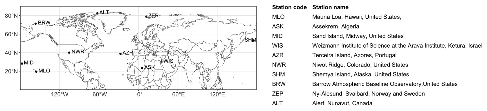
Figure 1 Map showing the location of studied sites, with the station names corresponding to the station code shown in the map.

Measurements of atmospheric CO₂ dry air mole fraction from remote background sites represent the balance between surface emissions and uptake from land and ocean (Keeling et al., 1996) over large spatial scales. The seasonal patterns evident in these data from the Northern Hemisphere reflect the terrestrial ecosystem exchange, mostly from the high and mid-latitudes, and have been used by previous studies to investigate the changes in the CUP_NEE over large spatial scales (e.g. Barichivich et al., 2012; Piao et al., 2008, 2017). Robust methods were developed for the estimation of the CUP from the CO₂ mixing ratio, such as the ensemble of first derivative (EFD) method from Kariyathan et al. (2023), which was better able to identify changes in the CUP_NEE compared to the conventional use of the dates when the detrended seasonal cycle crossed the zero value. Even with refined CUP_MR estimation methods, atmospheric transport causes a significant fraction of observed CO₂ variations at surface stations. Interannual variations and long-term trends in atmospheric transport can affect the relationship between the seasonal cycle of atmospheric CO₂ observations and surface exchange (Murayama et al., 2007; Piao et al., 2008). For example, Jin et al. (2022) studied the impact of varying winds and ecological CO₂ fluxes on seasonal cycle amplitude trends, finding that shifting winds partially offset the amplitude increase at Mauna Loa (MLO), contributing nearly 50 % to the seasonal cycle amplitude changes between 1959 and 2019. Lintner et al. (2006) suggest a contribution by atmospheric transport to the downward trend in the CO₂ seasonal cycle amplitude observed at MLO between 1991 and 2002. Murayama et al. (2007) demonstrated how year-to-year changes in atmospheric transport create significant interannual variations in the downward zero-crossing date of the CO₂ seasonal cycle, inevitably influencing CUP_MR estimates. Previous studies have primarily focused on aspects such as the seasonal cycle amplitude or zero-crossing times. Barlow et al. (2015) used the improved CUP estimation method to explore the influence of transport on CUP timing to some extent. In this study, we aim to understand in detail how well the CUP_MR deduced from atmospheric time series observations of CO₂ mixing ratios represents the CUP_MR changes from the Northern Hemisphere biosphere and its interannual variability (IAV), especially:

1. To what extent do CO₂ mixing ratio observations accurately capture variations in CUP_NEE?

2. How does IAV in atmospheric transport affect the observed changes in CUP_MR?

3. Considering the variability in both CUP_NEE and transport, can CUP_MR effectively reflect long-term trends in CUP_NEE?

4. Can the changes observed at the studied sites be attributed to specific regions of the Northern Hemisphere?

To address these questions, we evaluate the role of transport in shaping the CUP_MR at regional and global scales by conducting a series of experiments using the atmospheric transport model TM3 (Heimann and Körner, 2003) for a total of 10 sites in the Northern Hemisphere (Fig. 1).

2 Methods

To evaluate the degree to which CUP_MR represent the changes in the CUP_NEE, when influenced by atmospheric transport, we design idealized scenarios with prescribed changes to the optimized NEE fluxes from the Jena CarboScope Atmospheric CO₂ Inversion (Rödenbeck et al., 2003) (version ID: sEXTocNEET_v2021). The modifications were applied solely to pixels in the Northern Hemisphere (> 0° N) with a clearly defined seasonal cycle, characterized by a seasonal cycle minimum, and downward and upward zero-crossing points in spring and autumn, respectively. The year 2003 is employed as the reference year (simulations with an alternative reference year, 2001, did not show a noticeable difference), and pixels exhibiting clearly defined seasonal cycles in that specific year were chosen for perturbation. For the remaining pixels, the reference year flux was repeated over time, so that there was no IAV in CUP_NEE. This was done to ensure that any observed changes in the simulated CO₂ mixing ratio could be attributed to the prescribed Δ. The influence of fossil fuel, biomass burning, and ocean fluxes on the seasonal variation of atmospheric CO₂ is minimal, and changes in the seasonal cycle of atmospheric CO₂ reflect alterations in the integrated net ecosystem exchange in the Northern Hemisphere (Barichivich et al., 2012). While these fluxes were not modified in our simulations, our results are based on differences between simulations where only the NEE flux is altered. The flux manipulation was carried out from 1995 to 2017, aligning with the meteorological forcing used in the transport model. These adjusted fluxes were then transported forward using an atmospheric transport model, TM3 (Heimann and Körner, 2003), simulating time series of CO₂ mixing ratios at different study sites (as shown in Fig. 1), in temporal frequency aligning with the flask measurements at the sites. The 10 sites chosen for this study represent a selected subset of the Northern Hemisphere observation network. To minimize anthropogenic influences, only remote background sites were included. These sites were selected based on their long-term data records and their spatial distribution across the Northern Hemisphere, with roughly at least one station per 10° latitude, capturing the network's spatial diversity. Previous studies, such as Murayama et al. (2007) and Piao et al. (2008), have confirmed that interannual variations and long-term trends in atmospheric transport can affect the relationship between the seasonal cycle of atmospheric CO₂ observations and surface exchange. These studies also used a subset of background sites to evaluate transport influence on observed signals, similar to our approach. After the forward transport run, we assess CUP_MR changes based on the simulated CO₂ mixing ratios (ΔCUP_MR) resulting from ΔCUP_NEE. We use the EFD method from Kariyathan et al. (2023) to evaluate CUP_MR, as its efficacy on the sites shown in Fig. 1 was previously established in Kariyathan et al. (2023). The method uses an ensemble-based approach to quantify the uncertainty associated with curve-fitting discrete time series data and deriving seasonal cycle metrics. Using this approach, an optimal threshold is defined based on the first derivative of the CO₂ seasonal cycle to determine CUP timing. The threshold is selected such that the CUP timing closely corresponds to the spring maximum and late summer minimum, with minimal influence from curve-fitting uncertainty caused by multiple or broader peaks in the CO₂ seasonal cycle.

Table 1 Description of different forward simulation experiments using manipulated NEE fluxes. The first character in the experiment name indicates if the early (E) or late (L) CUP_NEE phases are manipulated, the next character specifies if Northern Hemisphere (N) or Regional (R) fluxes are adjusted, and the subscript and superscript of the last character denote variability (V) in CUP_NEE and transport, respectively. The Δ applied in each experiment is shown in the first column. In ${\mathrm{\Delta }}_x^{\mathrm{d}}$CUP_NEE, x ranges from −10 to +10 d in intervals of 2 d. In ${\mathrm{\Delta }}_x^{\mathrm{l}}$CUP_NEE, x can be a sequence from −10 to +10 d and vice versa denoted by p and n, respectively, in the main text.

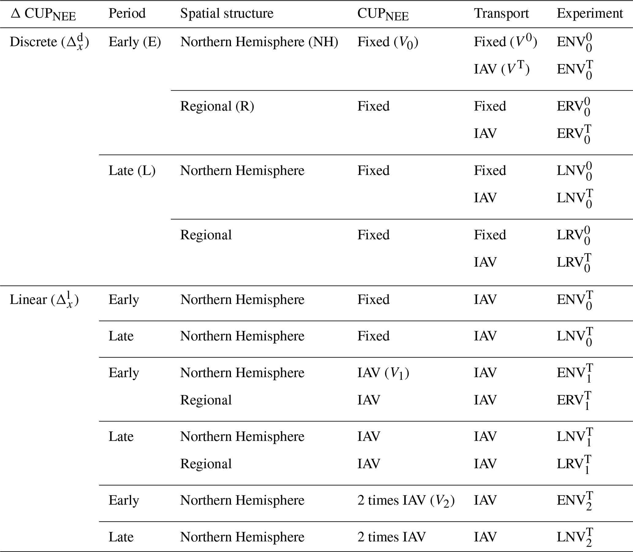
To evaluate how well CUP_MR captures the changes in CUP_NEE, we used experiments ${\mathrm{ENV}}_{\mathrm{0}}^{\mathrm{0}}$ and ${\mathrm{LNV}}_{\mathrm{0}}^{\mathrm{0}}$, where we imposed spatially uniform, discrete changes in CUP_NEE (Δ^d) and the atmospheric transport was held constant in the forward transport run (meaning that one year (2008) of transport was repeated). Then, to answer how the IAV in atmospheric transport affects derived CUP_MR, the CO₂ mixing ratios were simulated with interannually varying meteorology (experiment ${\mathrm{ENV}}_{\mathrm{0}}^{\mathrm{T}}$ and ${\mathrm{LNV}}_{\mathrm{0}}^{\mathrm{T}}$). To evaluate the ability of CUP_MR to reflect long-term trends in CUP_NEE, we initially assessed the ability to capture a trend in CUP_NEE while accounting for IAV in atmospheric mixing. This was achieved by prescribing long-term trends in CUP_NEE (Δ^l) and conducting the forward transport run with interannually varying meteorology. Subsequently, we then tested the detectability of prescribed linear trends in CUP_NEE (Δ^l) when IAV was present in both atmospheric transport and NEE (experiments ${\mathrm{ENV}}_{\mathrm{1}}^{\mathrm{T}}$ and ${\mathrm{LNV}}_{\mathrm{1}}^{\mathrm{T}}$). Additionally, to analyse the influence of IAV in CUP_NEE, we prescribed known IAV to CUP_NEE (experiments ${\mathrm{ENV}}_{\mathrm{2}}^{\mathrm{T}}$ and ${\mathrm{LNV}}_{\mathrm{2}}^{\mathrm{T}}$). Further, to understand the sensitivity of the simulated signals to regional changes (experiments ${\mathrm{ERV}}_{\mathrm{0}}^{\mathrm{0}}$, ${\mathrm{LRV}}_{\mathrm{0}}^{\mathrm{0}}$, ${\mathrm{ERV}}_{\mathrm{1}}^{\mathrm{T}}$, and ${\mathrm{LRV}}_{\mathrm{1}}^{\mathrm{T}}$), we limited the flux manipulation to Northern Hemisphere land regions of the TransCom3 (Gurney et al., 2002) experiment, namely Europe, Eurasian Temperate, Eurasian Boreal, North American Temperate, and North American Boreal. The experiments performed are listed in Table 1.

2.1 NEE flux manipulation

The CUP_NEE is the period when the NEE flux is negative, and the downward and upward zero-crossing dates represent the onset and termination of the CUP_NEE, respectively. Hence, we shift the NEE zero-crossing dates to have a change Δ (where Δ is measured in days) in the CUP_NEE duration (ΔCUP_NEE). The NEE flux is characterized by daily temporal resolution, showing relatively gradual variations along the y-axis compared to the x-axis. For all the experiments performed, the NEE values (i.e., y-axis) are modified to achieve the desired timing adjustments (Δ) in CUP_NEE without altering the time axis itself. This adjustment ensures the creation of a smooth curve that closely mirrors the actual flux while achieving the intended change in CUP_NEE. For each value of ΔCUP_NEE, we modify the downward and upward zero-crossing dates of NEE separately to evaluate the effect of changes in the early and late CUP_NEE phases, respectively. This is achieved by adding or subtracting a continuous curve to the period extending from the peak in spring to the NEE minimum for early phase changes and the period from the NEE minimum to peak in winter for late phase changes. The curve is created by combining two distinct half-Gaussian curves (Fig. 2, red and blue curves): the first curve has its peak at the new onset/termination and a standard deviation (σ₁) equal to one-third of the distance between the NEE peak in spring/winter and the new onset/termination. The second curve, also with its peak at the new onset/termination, has a different standard deviation (σ₂) equal to one-third of the distance between the new onset/termination and the date corresponding to the NEE minimum value. This configuration (i.e., Gaussian peaks and σ) ensures that the Gaussian tail minimizes any shift around the NEE peak and trough while realizing the Δ shift at the onset or termination of the CUP_NEE.

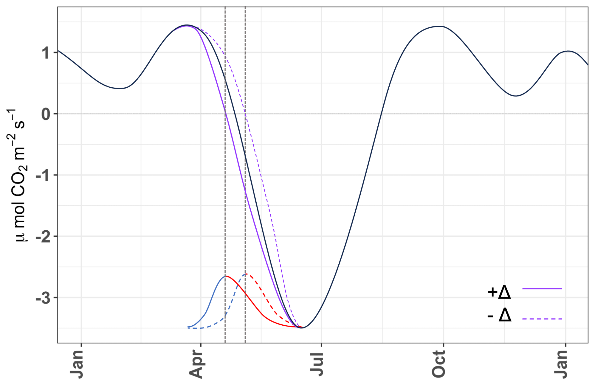
Figure 2 Schematic showing manipulation of CUP_NEE. The shifted purple solid/dashed curves result in +Δ and −Δ changes in the CUP_NEE, respectively. The curve is obtained by subtracting/adding two half-Gaussian curves. For example, the red and blue curves combine at the points (i.e., new onset) indicated by the dashed black lines to produce the purple curves (described in Sect. 2.3). The seasonal cycle minimum separates the early (left) and late (right) CUP_NEE phases. The manipulation for the early CUP_NEE phase is shown here and can be similarly applied to the late CUP_NEE phase.

Some pixels exhibit a distinct seasonal pattern without a well-defined peak in spring or winter. In those cases, the period for manipulating the early and late CUP phases then extends from the beginning of the year to the day of minimum NEE and from the day of minimum NEE to the end of the year, respectively. The portions of the first and second curves corresponding to the range from “μ−3σ₁” to “μ” and from “μ” to “μ+3σ₂”, respectively, are then combined and smoothed using a spline function (Fig. 2, purple curves).

We note that the annual flux is not conserved in the manipulation. However, we detrend the simulated CO₂ mixing ratio prior to CUP_MR analysis, which would remove any trend in the CO₂ mixing ratio caused by repetition of the manipulated years. Further, when evaluating the simulated CO₂ time series, we found that the change in the total annual flux only changes the peak-to-peak amplitude and does not influence the timing and duration of the simulated time series, except at times corresponding to periods of manipulation in the CUP_NEE. This happens, for instance, when the downward zero crossing of the NEE flux is manipulated: it changes only the CUP onset and has minimal influence on the CUP termination in the CO₂ mixing ratios. The different cases of manipulation are described below.

1. ${\mathrm{\Delta }}_x^{\mathrm{d}}$: In these simulations, every year has the same discrete change in CUP_NEE. In the different experiments, the magnitude of the shift (denoted by x) ranges from −10 to 10 d in intervals of 2 d.

2. ${\mathrm{\Delta }}_x^{\mathrm{l}}$: In these simulations, ΔCUP_NEE progresses from −10 to +10 d (denoted by x=p) or vice versa (denoted by x=n) over the period of manipulation.

Manipulation ${\mathrm{\Delta }}_x^{\mathrm{d}}$ is done for experiments where there is no IAV in CUP_NEE, indicated by V₀ in the experiment name. ${\mathrm{\Delta }}_x^{\mathrm{l}}$ manipulation is made for experiments with and without IAV in CUP_NEE (i.e., experiment names with V₀, V₁, and V₂). For the case V₀, the manipulation is done on the flux of a reference year (2003 chosen arbitrarily), which is repeated in time so that there is no IAV in CUP_NEE. Any IAV in CUP_MR may then be attributed to IAV in transport. In V₁, the annual fluxes are used instead of repeating the base year flux. The case V₂ has a prescribed IAV in CUP_NEE. In this case, for a given pixel, a set of Δ values is added to the original CUP_NEE in the manipulation period (2000–2017). The set of Δ has a mean zero and a standard deviation twice that of the IAV in the original CUP_NEE for the manipulation period.

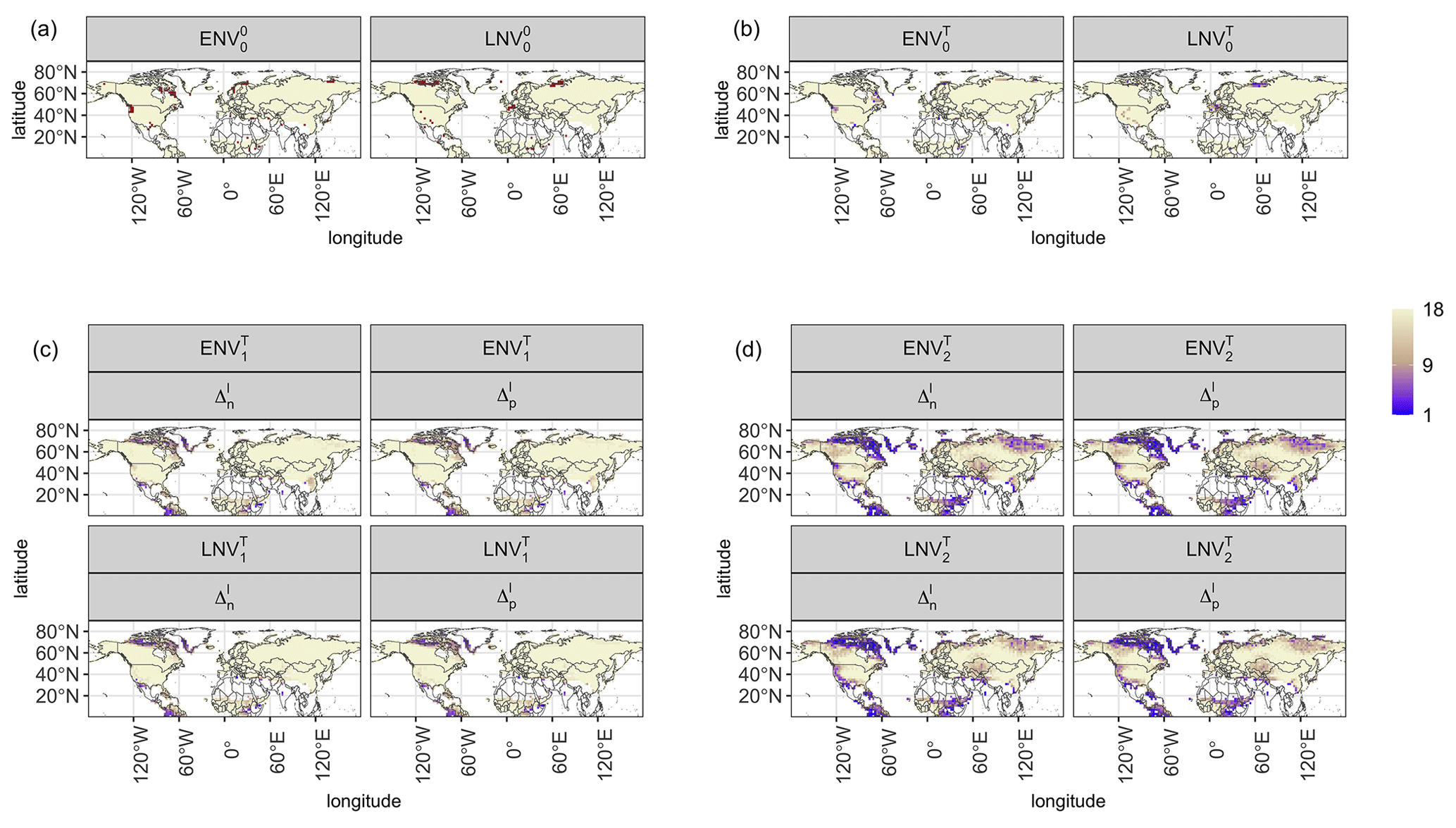
Figure 3 Spatial distribution of the pixels manipulated for different experiments. (a) Reference year flux is repeated and discrete changes are prescribed to CUP_NEE (beige), the red colour represents pixels where Δ is different from the prescribed Δ due to the complications described in Sect. 2.1. (b) Reference year flux is repeated and a long-term trend is applied to CUP_NEE. When a long-term trend is applied, Δ varies over the years. The colour bar indicates the number of years for which Δ equals the prescribed Δ, i.e., years with no complications described in Sect. 2.1 (also applicable for panels (c) and (d)). (c) Actual CUP_NEE is retained and long-term trend is applied to CUP_NEE. (d) IAV in CUP_NEE is doubled and a long-term trend is applied. The panel titles in every plot represent different simulations as detailed in Table 1.

The flux alteration is complicated to apply in some cases, as described below.

1. When a local maximum is observed between the downward or upward zero-crossing points and the minimum NEE. In such cases, adding the Gaussian curve shifts these peaks above the zero-crossing line, creating an additional downward or upward zero-crossing point. This complicates the assessment of CUP_NEE following the manipulation, and results in ΔCUP_NEE being different from the prescribed value. The Δ is kept at zero in this case.

2. In a few instances, when the magnitude of Δ is larger than the period between the original zero-crossing dates and the start/end of the period of manipulation, we instead opt for the next-closest Δ value in the sequence.

3. Additionally, in manipulation cases where interannually varying fluxes are used (${\mathrm{\Delta }}_x^{\mathrm{l}}$), only certain years have the complexities described above. In such instances, the next available Δ value from the sequence is chosen to minimally impact the imposed CUP_NEE trend. This involves selecting a Δ such that it results in a smaller or larger value compared to the subsequent year, achieving either a positive or negative change in CUP_NEE (i.e., ${\mathrm{\Delta }}_p^{\mathrm{l}}$ or ${\mathrm{\Delta }}_n^{\mathrm{l}}$CUP_NEE).

The manipulated pixels for the different cases are shown in Fig. 3. Furthermore, the manipulated fluxes are used to conduct regional sensitivity analyses, in which we limit the flux manipulation process explained above to different TransCom3 (Gurney et al., 2002) geographic regions in the Northern Hemisphere. This allows us to evaluate the regional contribution of NEE fluxes to ΔCUP_MR when comparing how perturbations involving different regions are expressed in ${\mathrm{\Delta }}_x^{\mathrm{l}}$CUP_MR at the studied sites. This comparison is conducted for two experiments: ${\mathrm{ERV}}_{\mathrm{0}}^{\mathrm{0}}$, illustrating the integration of signals from various regions in an idealized scenario without IAV in atmospheric transport or CUP_NEE; and ${\mathrm{ERV}}_{\mathrm{1}}^{\mathrm{T}}$, which reflects signal integration in a relatively realistic setting, with IAV in atmospheric transport and CUP_NEE.

2.2 Forward transport runs

We use a three-dimensional global atmospheric transport model, TM3 (Heimann and Körner, 2003), to simulate CO₂ mixing ratios at the specified sites based on manipulated NEE fluxes. The model is run at a spatial resolution of 5° in longitude and 4° in latitude with 19 vertical levels, using 6-hourly NCEP reanalysis meteorological fields from 1995 to 2017 and daily surface fluxes from the Jena CarboScope CO₂ Inversion (version ID: sEXTocNEET_v2021) (Rödenbeck et al., 2003), with the NEE fluxes manipulated as previously described. The forward runs are carried out with (1) fixed transport (meteorology from a random year, here we used the year 2008 and repeated it in time such that there is no IAV) and (2) interannually varying transport for the period 1995 to 2017 to study the contribution of atmospheric transport to the IAV in CUP_MR. The first five years are excluded from the CUP_MR analysis to account for the model's spin-up time, and ΔCUP_NEE is held at zero during this period.

2.3 CUP estimation methods

The forward transport runs simulate CO₂ mixing ratios at discrete time steps, which we sample at the frequency corresponding to the flask measurements (approximately bi-weekly) at the studied sites. This sampling interval sufficiently captures the larger-scale trends and seasonal variations critical to our analysis and allows for consistent comparison with previous studies that looked into long-term trends using flask measurements. We apply the EFD method described in Kariyathan et al. (2023) to the output data and estimate the CUP_MR. Here, the CUP_MR is estimated using a threshold derived from the first derivative of the detrended and smoothed CO₂ mixing ratio seasonal cycle curves. A threshold of 15 % and 0 % of the first-derivative minimum was used as a threshold to determine the onset and termination of the CUP_MR, respectively, as in Kariyathan et al. (2023). The calculation is applied to an ensemble of the detrended time series, which allows for an uncertainty range on the CUP estimate to be calculated.

3 Results

3.1 Northern Hemisphere CUP_MR sensitivity under fixed transport

The calculated ΔCUP_MR consistently shows lower absolute values than the prescribed ΔCUP_NEE. For example, at BRW, ΔCUP_MR is 0.43 times the prescribed early phase ΔCUP_NEE as illustrated in Fig. 4a. This reduction in ΔCUP_MR is found across all the studied sites with varying degrees of intensity, as illustrated in Fig. 4d, when Δ is prescribed to either the early or late phases of CUP_NEE. This shows how atmospheric observations respond differently to CUP perturbations compared to local NEE measurements, and a one-on-one translation might lead to an incorrect interpretation of at least the magnitude of CUP changes. The persistent difference in the magnitude of ΔCUP_MR from the imposed ΔCUP_NEE results from the integration of signals from various regions with different CUP_NEE timings as detailed in Sect. 4.

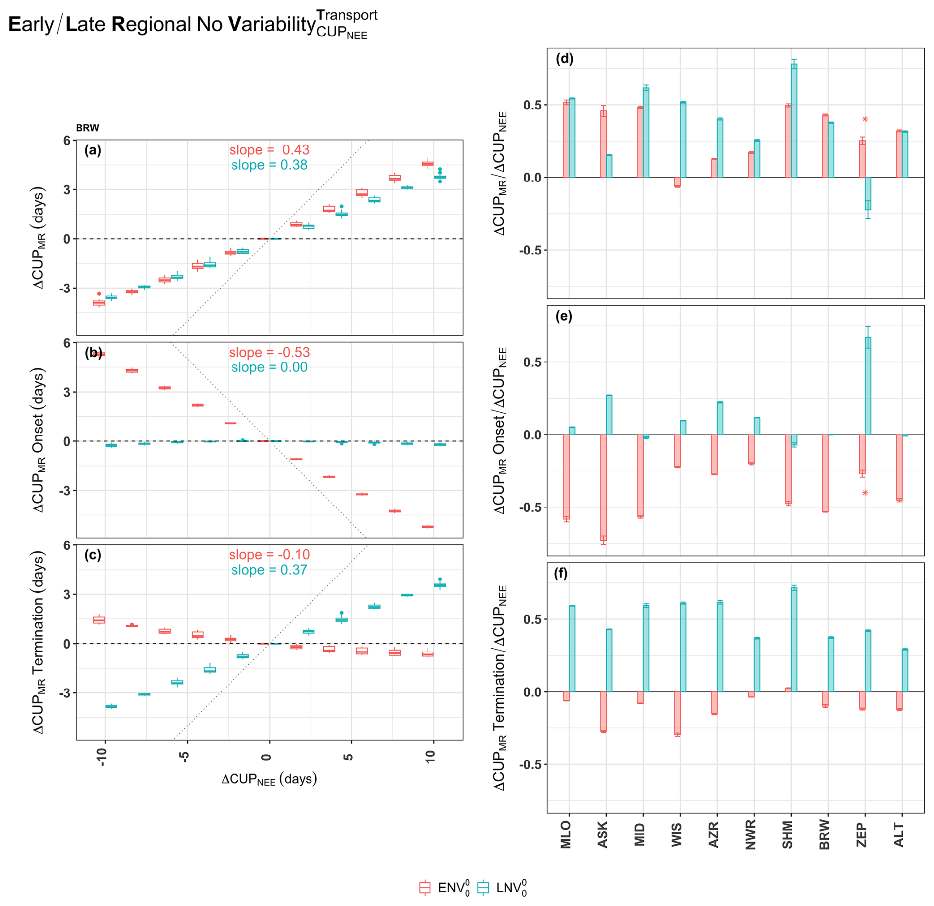
Figure 4 The change in CUP_MR in response to varying ΔCUP_NEE for experiments ${\mathrm{ENV}}_{\mathrm{0}}^{\mathrm{0}}$ (red) and ${\mathrm{LNV}}_{\mathrm{0}}^{\mathrm{0}}$ (cyan). The experiments ${\mathrm{ENV}}_{\mathrm{0}}^{\mathrm{0}}$ and ${\mathrm{LNV}}_{\mathrm{0}}^{\mathrm{0}}$ largely drive the Δ in CUP_MR onset and termination, respectively, and thereby ΔCUP_MR. The left panels show the Δ in (a) CUP_MR (i.e., the duration), (b) CUP_MR onset, and (c) CUP_MR termination against the applied ΔCUP_NEE for BRW. In these panels, the individual boxplots display the distribution of the median values across years, estimated from the ensemble spread for each year. The dotted line represents an ideal case of a one-to-one (minus one-to-one for panel (b)) relation between ΔCUP_NEE and ΔCUP_MR. The text within these plots shows the slope of the regression lines fitted to the median of the boxplots. The right panels (d–f) show these slopes (unitless) across the different studied sites. The estimate of ZEP is reduced to 0.1 times the actual value for ease of visualization. Error bars represent ±1 standard deviation (σ) around the estimated slope.

At most studied sites, the Δ assigned to the early phase of CUP_NEE predominantly affects the onset of CUP_MR (Fig. 4b and e). The ΔCUP_MR then corresponds to the changes in onset of CUP_MR as indicated by the similar variation in the red bars in Fig. 4d and e. Similarly, Δ applied to the late phase of CUP_NEE primarily influences the termination of CUP_MR (Fig. 4c and f) which then drives ΔCUP_MR in experiment ${\mathrm{LNV}}_{\mathrm{0}}^{\mathrm{0}}$ (Fig. 4d and f, cyan bars). This suggests that the changes in the early and late phases of CUP at the surface can be analysed separately by examining the onset and termination of CUP inferred from CO₂ mole fraction observations. Contrary to the direct but dampened relationship between ΔCUP_NEE and ΔCUP_MR, we find an opposite response at some sites: a lengthening (shortening) imposed on CUP_NEE leads to shortening (lengthening) of the CUP_MR. This is seen to occur at sites ZEP and WIS, as indicated by the negative slopes at these sites (Fig. 4d).

At ZEP, the late phase ΔCUP_NEE leads to unintended changes in CUP_MR onset. For Δ prescribed to the late CUP_NEE phase, the change in CUP_MR termination is only 0.4 times the Δ, while that in the onset is 0.6 times the Δ. Thus, the changes intended for CUP_MR termination extend to CUP_MR onset in the following year. For example, a 10 d delay prescribed to the CUP_NEE termination results in a 4 d delay in CUP_MR termination and a 6 d delay in the onset. This results in a 2 d shorter CUP_MR, establishing an inverse relation between ΔCUP_MR and ΔCUP_NEE at ZEP (slope of −0.22 in the experiment ${\mathrm{LNV}}_{\mathrm{0}}^{\mathrm{0}}$). Likewise, at WIS, in experiment ${\mathrm{ENV}}_{\mathrm{0}}^{\mathrm{0}}$, the change in CUP_MR onset is only −0.2 times the applied early phase ΔCUP_NEE, while the change in termination is −0.3 times the perturbation imposed. This offsets the ΔCUP_MR and leads to a significant (p < 0.001) inverse relation between ΔCUP_MR and ΔCUP_NEE at WIS (slope of −0.06, in the ${\mathrm{ENV}}_{\mathrm{0}}^{\mathrm{0}}$ experiment).

3.2 Northern Hemisphere CUP_MR sensitivity under interannually varying transport

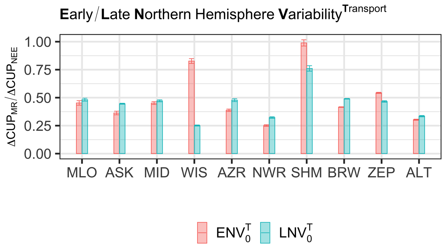
Even when interannual variations from atmospheric transport are included, changes imposed in ΔCUP_NEE are reflected in ΔCUP_MR. The varying atmospheric transport leads to year-to-year variations in signal integration and changes that were not captured in the experiment with transport from single-year meteorology can be seen in the experiment with interannually varying transport. This is illustrated for different sites in Fig. 5. An inverse relation between ΔCUP_MR and ΔCUP_NEE was calculated at WIS and ZEP in experiments ${\mathrm{ENV}}_{\mathrm{0}}^{\mathrm{0}}$ and ${\mathrm{LNV}}_{\mathrm{0}}^{\mathrm{0}}$, respectively, as described in Sect. 3.1. However, in experiments with varying transport, slope values of 0.83 at WIS (experiment ${\mathrm{ENV}}_{\mathrm{0}}^{\mathrm{T}}$) and 0.47 at ZEP (experiment ${\mathrm{LNV}}_{\mathrm{0}}^{\mathrm{T}}$) are found, compared to −0.06 and −0.22 in the experiment with fixed transport. This suggests that anomalies observed in specific years may be predominantly attributed to the meteorological conditions of those particular years.

Figure 5 The change in CUP_MR metrics in response to varying ΔCUP_NEE, similar to Fig. 4d but for the experiments with interannually varying meteorology, ${\mathrm{ENV}}_{\mathrm{0}}^{\mathrm{T}}$ (red) and ${\mathrm{LNV}}_{\mathrm{0}}^{\mathrm{T}}$ (cyan).

3.3 Northern Hemisphere CUP_MR sensitivity to long-term trends in CUP_NEE

Out of all the evaluated sites, only SHM and BRW partially captured CUP_MR trends corresponding to the imposed trends in CUP_NEE as shown in Fig. 6 (results for other sites are shown in Table A1). In experiment ${\mathrm{ENV}}_{\mathrm{0}}^{\mathrm{T}}$, the largest trend in CUP_MR is derived at SHM, with values of 0.5 and −0.3 d yr⁻¹ for the imposed increasing (1.11 d yr⁻¹) and decreasing (−1.11 d yr⁻¹) trend, respectively. Similarly, in experiment ${\mathrm{LNV}}_{\mathrm{0}}^{\mathrm{T}}$, the largest trend in CUP_MR is observed at BRW (0.5 and −0.2 d yr⁻¹ for the imposed increasing and decreasing trend, respectively). Nevertheless, part of the observed trend can be attributed to the IAV in atmospheric transport, thereby showing that the IAV in transport can influence our understanding of the actual long-term changes in CUP_NEE trends. This can be seen in Fig. 6, green bars (${\mathrm{\Delta }}_{\mathrm{0}}^{\mathrm{l}}$), corresponding to experiments ${\mathrm{ENV}}_{\mathrm{0}}^{\mathrm{T}}$ and ${\mathrm{LNV}}_{\mathrm{0}}^{\mathrm{T}}$. Note that in these experiments, there is no IAV in the CUP_NEE flux as indicated by the subscript “0”, and ${\mathrm{\Delta }}_{\mathrm{0}}^{\mathrm{l}}$ indicates that no trend is prescribed to the CUP_NEE. Then any derived CUP_MR trend can be attributed solely to the IAV in transport. The trend from the IAV in transport contributes to the asymmetry between the red and blue bars. At BRW, experiment ${\mathrm{LNV}}_{\mathrm{0}}^{\mathrm{T}}$, indicates that a CUP_MR trend of 0.1 d yr⁻¹ can arise from variability in transport alone, and accounts for about 20 % of the derived CUP_MR trend (blue bar showing 0.5 d yr⁻¹).

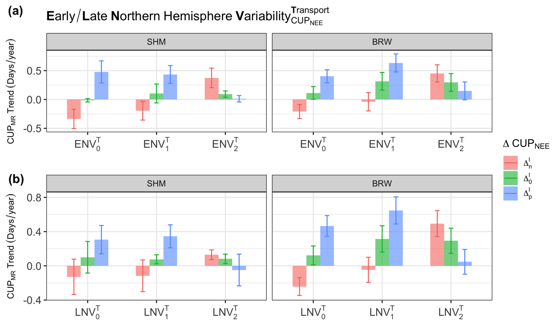
Figure 6 Sensitivity of CUP_MR to the applied long-term trend in CUP_NEE (results for sites SHM and BRW). The bars show the slope of the regression line fitted to the median CUP_MR from experiments ${\mathrm{ENV}}_x^{\mathrm{T}}$ (a) and ${\mathrm{LNV}}_x^{\mathrm{T}}$ (b), where x is 0, 1, and 2 implying no IAV in NEE flux, the actual IAV in NEE flux, and two times the actual IAV in NEE flux, respectively. Error bars represent ±1 standard deviation (σ) around the estimated slope. Colours show the prescribed trend ${\mathrm{\Delta }}_p^{\mathrm{l}}$ (1.1 d yr⁻¹) in blue, ${\mathrm{\Delta }}_n^{\mathrm{l}}$ (−1.1 d yr⁻¹) in red, and ${\mathrm{\Delta }}_{\mathrm{0}}^{\mathrm{l}}$ (0 d yr⁻¹) in green applied to CUP_NEE.

Furthermore, we observe that the actual IAV in the CUP_NEE fluxes contribute to the derived CUP_MR trends; however, as the IAV in the flux becomes larger, it imposes noise that makes the trends harder to detect. This is shown in experiments ${\mathrm{ENV}}_{\mathrm{1}}^{\mathrm{T}}$ and ${\mathrm{ENV}}_{\mathrm{2}}^{\mathrm{T}}$ (Fig. 6), where the actual IAV in CUP_NEE is retained and doubled, respectively. In experiment ${\mathrm{ENV}}_{\mathrm{1}}^{\mathrm{T}}$, the CUP_MR trend in response to the prescribed opposite trends, ${\mathrm{\Delta }}_p^{\mathrm{l}}$ and ${\mathrm{\Delta }}_n^{\mathrm{l}}$ are distinct in sign. Even though the magnitude of the prescribed trend is the same, a large difference in magnitude can be seen between results for ${\mathrm{\Delta }}_p^{\mathrm{l}}$ (red bar, 0.6 d yr⁻¹) and ${\mathrm{\Delta }}_p^{\mathrm{l}}$ (blue bar, −0.03 d yr⁻¹), for example, at BRW. This can be attributed to the increasing trend from both IAV in the actual flux and transport, as indicated by the green bar for ${\mathrm{ENV}}_{\mathrm{1}}^{\mathrm{T}}$. The green bars in experiment ${\mathrm{ENV}}_{\mathrm{1}}^{\mathrm{T}}$ (0.3 d yr⁻¹) and ${\mathrm{ENV}}_{\mathrm{0}}^{\mathrm{T}}$ (0.1 d yr⁻¹) are distinct, and their difference (0.2 d yr⁻¹) is the contribution from the actual IAV in CUP_NEE alone. In the experiment where the IAV in CUP_NEE per pixel was doubled, it becomes evident that the imposed alterations in CUP_NEE are not accurately reflected in CUP_MR, even at sites like BRW, which exhibited pronounced responses in other experiments (${\mathrm{ENV}}_{\mathrm{1}}^{\mathrm{T}}$ and ${\mathrm{LNV}}_{\mathrm{1}}^{\mathrm{T}}$).

3.4 Regional contribution to CUP_MR

The various Transcom3 regions of the Northern Hemisphere contribute in various degrees to the CUP_MR changes observed at the studied sites. The changes in the Boreal regions are partially captured at both the higher and lower latitudes (e.g., ALT, BRW, SHM, MID, and MLO). Considering both the early and late ΔCUP_NEE phases, the contribution from the Eurasian Boreal region is largely seen at SHM (−3 d in the early and −7 d in the late CUP_NEE phase), followed by MID with (−3 in both the days early and late CUP_NEE phase), showing an eastward transport from the Eurasian Boreal region. Similarly, considering both the CUP_NEE phases, the contribution from the North American Boreal region is seen at all sites except ASK, WIS, and ZEP. In response to delayed onset, prescribed to the CUP_NEE in Eurasian Boreal region, a longer CUP_MR is calculated at ASK, WIS, and AZR (Fig. 7a), suggesting that the inverse slope relation between ΔCUP_MR and ΔCUP_NEE in Sect. 3.1 might largely be from changes in the Eurasian Boreal region. In the Eurasian Temperate region, the Δ prescribed to both the early and late CUP_NEE phases integrates at the lower latitude site (e.g., MID, MLO, NWR, and, SHM), whereas higher-latitude sites (e.g., ALT, BRW, and ZEP) only capture perturbations imposed during the early phase of CUP_NEE. The contribution from the North American Temperate region is strong during the early phase of CUP_NEE, while late phase changes are captured only by MID and AZR. Signals from the European region integrate well at most of the studied sites. At ZEP, a significant regional contribution from any of the studied TransCom3 regions can only be seen in the early CUP_NEE phase. This explains to some extent the direct relation between ΔCUP_MR and ΔCUP_NEE found only in the early phase (Sect. 3.1).

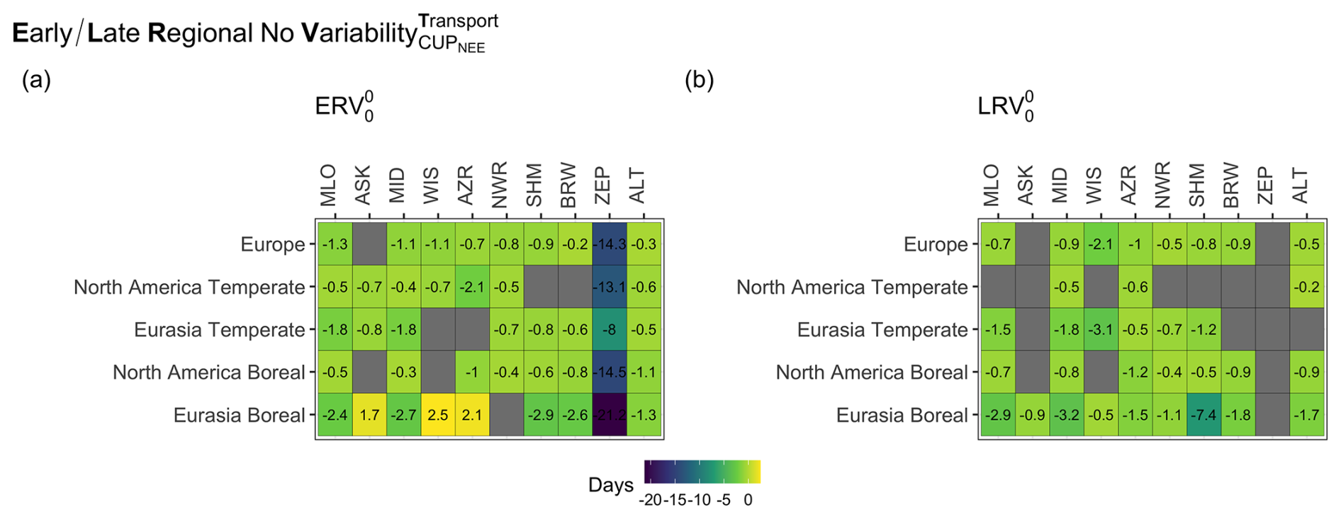
Figure 7 Regional contribution to ΔCUP_MR. The colour and value represent the ensemble median of ΔCUP_MR when ΔCUP_NEE is −10 d, in experiments ${\mathrm{ERV}}_{\mathrm{0}}^{\mathrm{0}}$ (a) and ${\mathrm{LRV}}_{\mathrm{0}}^{\mathrm{0}}$ (b). Values are displayed solely for the sites where a significant difference in ΔCUP_MR is detected when ΔCUP_NEE is 0 and −10 d (p-value of Mann–Whitney test < 0.05) in the specific region (y-axis).

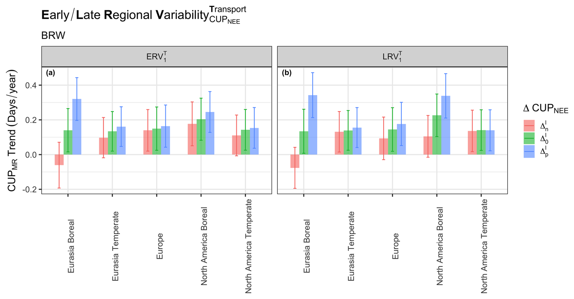
Figure 8 Regional contribution to CUP_MR trend detected at BRW in response to imposed long-term CUP_NEE trends. The bars show the slope of the regression line fitted to median CUP_MR from experiments ${\mathrm{ERV}}_{\mathrm{1}}^{\mathrm{T}}$ (a) and ${\mathrm{LRV}}_{\mathrm{1}}^{\mathrm{T}}$ (b). Error bars represent ±1 standard deviation (σ) around the estimated slope. The colours represent the trend in NEE imposed in the experiment, as described in Fig. 6.

The long-term trend in the CUP_MR could not be accurately attributed to different regions even for sites like BRW that showed a predominant response to the prescribed long-term trend in CUP_NEE (Sect. 3.3). This can be seen from Fig. 8. At BRW, the CUP_MR trends partially reflect the CUP_NEE trends prescribed to the Eurasian Boreal region. For example, in the early CUP_NEE phase, we find a change of 0.32 and −0.06 d yr⁻¹ in response to the prescribed ${\mathrm{\Delta }}_p^{\mathrm{l}}$ (1.1 d yr⁻¹) and ${\mathrm{\Delta }}_n^{\mathrm{l}}$ (−1.1 d yr⁻¹), respectively. However, the large error bars show that the uncertainty in trend estimation is large when changes are prescribed to only a given TransCom3 region.

4 Discussion

We find that changes (both fixed differences and trends) prescribed to CUP_NEE are reflected in CUP_MR simulated by TM3. However, the magnitude of the change seen in CUP_MR is consistently lower than the prescribed change in CUP_NEE, for example at BRW only about 50 % of the change applied to CUP_NEE was reflected in ΔCUP_MR, even in simulations with fixed transport. This is contradictory to previous studies that consider the long-term CO₂ record to reflect changes in surface fluxes. For example, in Piao et al. (2008), 50 % of the observed zero-crossing date variance at BRW could be accounted for by NEE variability.

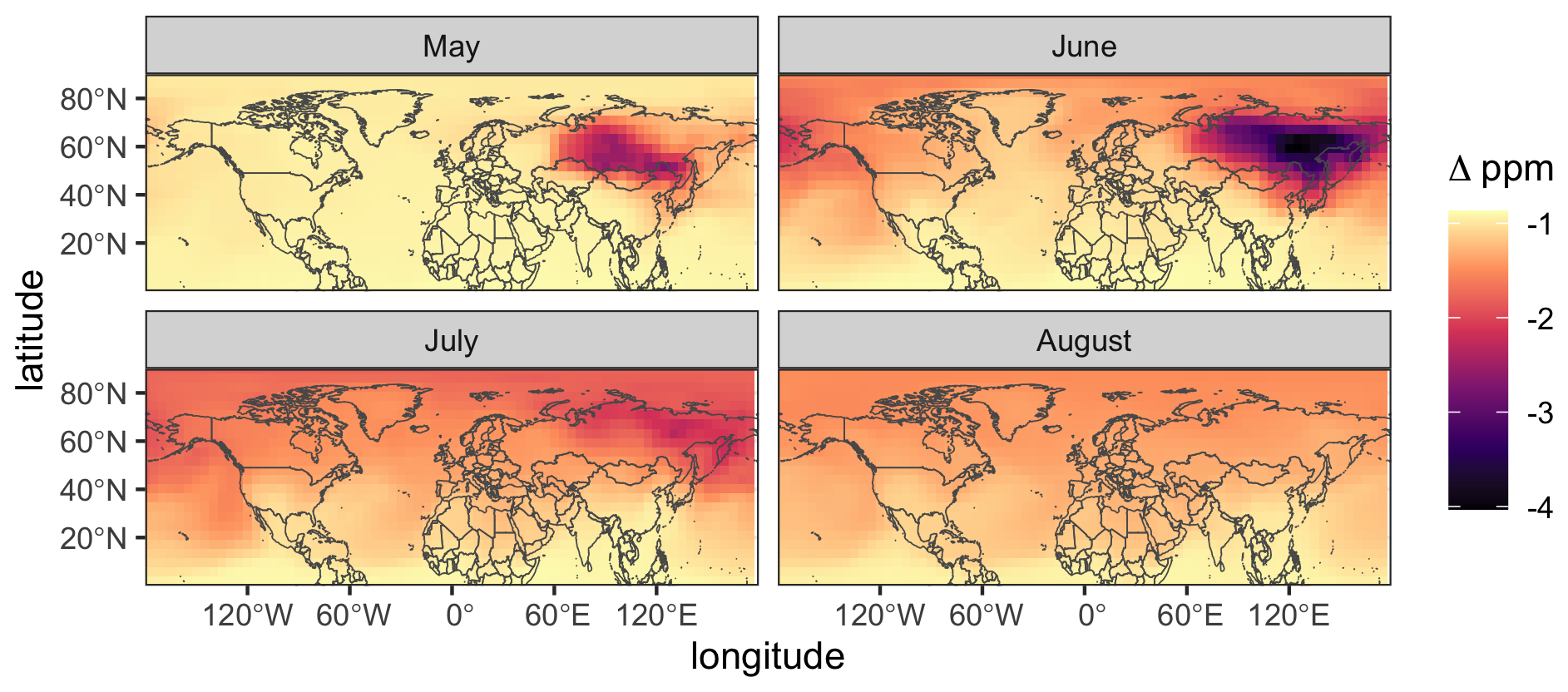
Figure 9 2D mixing ratio fields (integrated vertically up to an altitude of 400 m and averaged per month) when a delay of 10 d is prescribed to the CUP_NEE onset in the Eurasian Boreal region. The field (Δ ppm) is the difference between the 2D mixing ratio fields when ΔCUP_NEE is −10 and 0 d in experiment ${\mathrm{ERV}}_{\mathrm{0}}^{\mathrm{0}}$.

We show that, given fixed transport, the reduced expression of changes in CUP_MR relative to CUP_NEE arises from variations in the timing of CUP_NEE across the regions over which the signal is integrated. For instance, when a delay (10 d) was applied to the CUP_NEE onset in the Eurasian Boreal region, the mixing ratio reflects this change over the region in May and the signal slowly propagates eastward by June (Fig. 9), showing a difference in timing of the onset within the Eurasian Boreal region. The difference in the spatial distribution of CUP_NEE onset, with an earlier CUP_NEE onset in the western and later in the eastern part of the Eurasian Boreal region, is shown in Fig. 10. Due to the difference in CUP_NEE timing across the pixels, the effective ΔCUP_NEE of a region will be different from the applied Δ. The atmospheric transport does not always carry the CUP_NEE fluxes from the region to the observation site; it could be transported in other directions at other times. If an applied Δ shifts the CUP_NEE timing of some pixels into a period when transport is less favourable, the contribution from those pixels may be weaker or absent in the final measurements, causing a dampened relation between ΔCUP_NEE and ΔCUP_MR. Below, we discuss how the sensitivity of CUP_MR to the discrete and long-term changes in surface fluxes is affected when influenced by the interannual variability in both transport and surface fluxes.

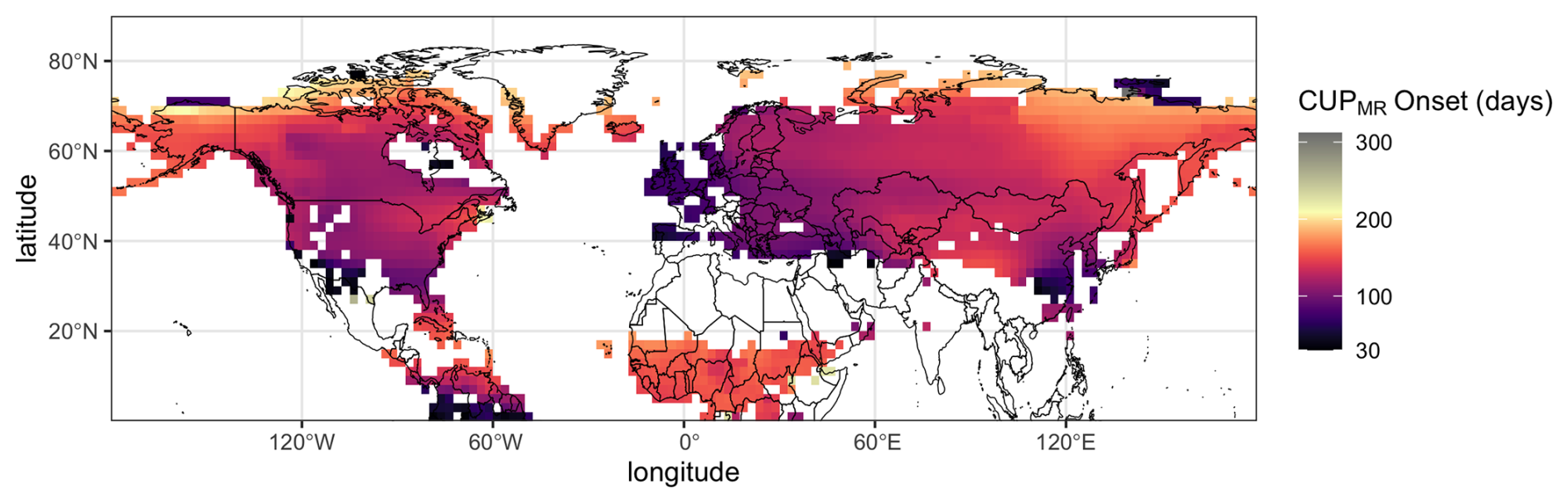
Figure 10 Spatial distribution of the CUP_NEE timing across the Northern Hemisphere as derived from Jena CarboScope CO₂ Inversion (version ID: sEXTocNEET_v2021) NEE fluxes for the reference year (2003) used in the study.

4.1 Transport influence on CUP_MR

We have shown the significant role of interannually varying atmospheric transport in the evaluation of metrics derived from CO₂ mole fraction data. At certain sites such as ZEP and WIS, the CUP_MR from simulations with fixed transport failed to capture the CUP_NEE changes, whereas in simulations with varying transport, the prescribed CUP_NEE changes could be partially derived from CUP_MR. This indicates that in a given year of meteorology used in the fixed transport simulation, the atmospheric transport is unlikely to originate from the areas where the ΔCUP_NEE was prescribed, while in simulations with transport variability, the meteorology in other years might have originated from these regions. Thus, the anomalies observed in CUP_MR in a particular year could stem from transport variability rather than anomalies in CUP_NEE itself, rendering mixing ratio time-series less useful for studying interannual variations in CUP_NEE.

Finally, we show that due to the atmospheric transport, the source areas for a given station during the early and late CUP_NEE phases can be substantially different, influencing the expression of CUP_MR in the different CUP_NEE phases. For instance, our analysis (Fig. 7) shows that WIS mainly receives signals from the Northern Hemisphere land pixels only in the late CUP_NEE phase. Consequently, at WIS, the CUP_MR is directly proportional solely to changes prescribed to late CUP_NEE phase (slope of 0.5 in ${\mathrm{LNV}}_{\mathrm{0}}^{\mathrm{0}}$). Similarly, at ZEP, the contribution of the Northern Hemisphere landmass to ΔCUP_MR occurs only in the early CUP_NEE phase. The atmospheric transport to ZEP is dominated by the regions Eurasian Boreal and Europe during March–May; in the following months (June–August), the air mass transport is largely confined to the Arctic and does not extend equatorward into the continents in some years (Tunved et al., 2013; Platt et al., 2022). Our observations imply that at ZEP/WIS, changes in the onset/termination of CUP_NEE are more effectively reflected as changes in CUP_MR.

4.2 Long-term trends in CUP_MR

The long-term trends prescribed to the CUP_NEE could be partially derived from CUP_MR at BRW and SHM, even under IAV in atmospheric transport and CUP_NEE. However, when IAV in CUP_NEE was doubled, the prescribed trends were not captured. This suggests that the long-term trends in the observations may be compromised when there is a higher IAV in CUP_NEE. The contribution from atmospheric transport exhibited a CUP_MR trend of 0.11 d yr⁻¹ at BRW. This finding aligns with a study by Murayama et al. (2007) where the IAV in transport alone caused a change of 0.16 d yr⁻¹ in the downward zero-crossing date at BRW for their analysis period between 1979 and 1999.

With warming, a longer growing season is observed in the high latitudes (e.g., Park et al., 2016, 2.6 d per decade). A longer growing season does not necessarily mean an increase in CUP_NEE or CUP_MR as they are determined by both photosynthesis and respiration. The existing literature on the CUP_NEE changes in the Northern Hemisphere based on CUP_MR varies from increasing (Keeling et al., 1996) to neutral (Barichivich et al., 2012) to decreasing (Piao et al., 2008). The complications in interpreting CUP_NEE changes arise mostly when directly assessing the CUP from CO₂ mixing ratio. Therefore, CO₂ observations should preferably be interpreted following a formal inverse estimate of the corresponding surface NEE. It is then possible to account for the interannual variability, trends, and delays imposed by the slow atmospheric mixing. Nevertheless, the ability of such inversions to constrain regional changes in NEE can only be improved with an expanded observation network.

4.3 Regional contribution to CUP_MR

The regions contributing to the integrated signal at various observation sites are influenced by atmospheric transport to these locations. From the idealized simulations with no IAV in transport or CUP_NEE it turned out that at sites like ALT, BRW, SHM, and MLO, a significant contribution from Boreal and Temperate regions could be calculated, indicating that these remote sites receive well-mixed signals from higher- and mid-latitude regions in the Northern Hemisphere with strong seasonality. We calculate that the contribution from mid-latitude is significant at the sites in the Boreal region (e.g., ALT and BRW in the early CUP_NEE phase) in line with Barnes et al. (2016). They found that the seasonal cycle observed at higher latitude sites is most sensitive to changes in the seasonality of mid-latitude surface emissions; however, we do not find that the mid-latitude influence is more than the Boreal region influences at higher-latitude sites. At ZEP, strong signals from both Eurasian and North American regions dominate during the early CUP_NEE phase (Fig. 7), and an amplification of the CUP_MR signal is found. Further, a significant change in the regional contribution is found between the early and late CUP_NEE phases, shifting from continental in the early CUP_NEE phase to ocean signals in parts of the late CUP_NEE phase (Sect. 4.1). This change explains the significant difference in ΔCUP_MR to ΔCUP_NEE during different phases, as shown in Fig. 4. At WIS, ASK, and AZR, when a delayed onset is imposed on the CUP_NEE from Eurasian Boreal regions, a positive ΔCUP_MR (i.e., an extension in CUP_MR) is calculated. These sites are located in the temperate regions. The CO₂ 2D mixing ratio fields (Fig. 9) reveal that changes imposed on the Boreal region propagate partially to the lower latitudes (around 30° N) later in the CUP_NEE phase. Thereby the delay imposed on the CUP_NEE of the Eurasian Boreal region in May integrates at the lower latitude region (near to the location of WIS, ASK, and AZR) only later in July, delaying and extending the CUP_MR.

When the long-term trends were applied to specific regions, the slope estimated from CUP_MR had large uncertainty due to the influence of IAV in transport and CUP_NEE. Furthermore, the flux manipulation strictly within the boundaries of the TransCom3 region in our experiments may have substantially limited the regions from which the signals reach the sites. In the real world, regional boundaries are more diffuse, and the footprint of the site provides a more accurate estimate of the regions contributing to the observed signals. Nonetheless, this aspect falls outside the scope of the present study.

The changes in the CO₂ mixing ratio time series from the Northern Hemisphere give a larger spatial perspective of the CUP_NEE changes. However, results from idealized simulations suggest that they are influenced by atmospheric transport IAV, seasonal changes in atmospheric transport, and IAV in the biospheric fluxes. We find a significant damping of the changes that were imposed on the CUP_NEE from the integration of signals from different regions that have varied timing and suggest a more intense change in the local spatial scales. With the constraints in NEE flux manipulation, imposed by the presence of local maxima and insufficient data points for Δ changes in the early and late CUP_NEE (Sect. 2.1), the simulations in this study do not accurately represent the real-world scenarios. In the real world, the changes in CUP_NEE are asynchronous across space. Although we broadly examined the influence of different TransCom3 regions, conducting more dedicated footprint analyses of the studied sites may offer further insights into the signals studied here.

5 Conclusions

Our analysis, based on forward model experiments, reveals that at well-studied sites such as MLO, BRW, and ALT, only circa 50 % of the prescribed changes in the CUP_NEE fluxes were reflected in CUP_MR. In simulations with interannually varying meteorology, the signals were better captured at a few sites like ZEP and WIS, showing the significant influence of IAV in atmospheric transport. At BRW, 20 % of the observed trend could be attributed to the IAV in transport. Furthermore, our findings suggest that the changes estimated in CUP_MR, subsequent to the separation of atmospheric transport influence, are likely to underestimate the actual magnitude of signals from the surface changes. This is because of the damping due to the integration of asynchronous CUP_NEE timing across different regions. While sites like BRW and SHM partially captured the prescribed long-term changes in the presence of natural IAV, they proved insensitive when IAV in CUP_NEE was doubled due to insufficient signal to noise. Furthermore, trends prescribed to individual TransCom3 regions were not captured by the evaluated sites, showing that long-term changes in the seasonal cycle of time series primarily reflect changes on larger spatial scales. These findings are based on forward model experiments rather than direct atmospheric observations, and they do not provide a direct estimate of biospheric changes. Instead, they highlight how atmospheric transport processes influence the representation of surface flux changes in CO₂ observations.

Appendix A

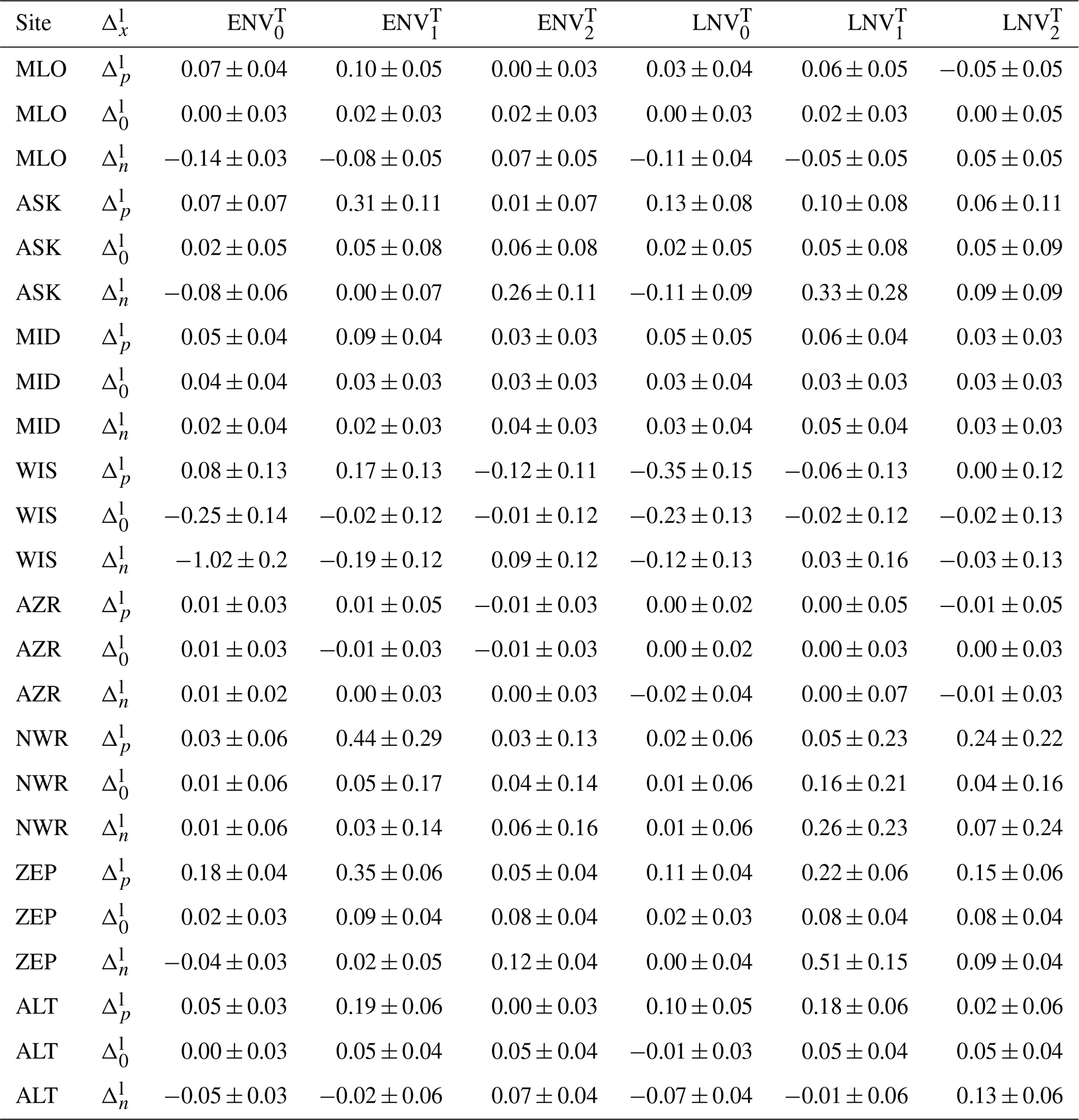
Table A1 Sensitivity of CUP_MR to the applied long-term trend in CUP_NEE for the different sites (excluding SHM and BRW). The first column shows the sites, the second column describes the prescribed trend ${\mathrm{\Delta }}_x^{\mathrm{l}}$ applied to CUP_NEE, and the other columns describe the different experiments, as detailed in the caption of Fig. 6. The values show the slope of the regression line fitted to the median CUP_MR ±1 standard deviation (σ) around the estimated slope (in units of d yr⁻¹) for the experiments indicated by the column names.