Global CH₄ fluxes derived from JAXA/GOSAT lower-tropospheric partial column data and the CarbonTracker Europe-CH₄ atmospheric inverse model

Satellite-driven inversions provide valuable information about methane (CH₄) fluxes, but the assimilation of total column-averaged dry-air mole fractions of CH₄ (XCH₄) has been challenging. This study explores, for the first time, the potential of the new lower-tropospheric partial column (pXCH₄_LT) GOSAT data, retrieved by the Japan Aerospace Exploration Agency (JAXA), to constrain global and regional CH₄ fluxes. Using the CarbonTracker Europe-CH₄ (CTE-CH₄) atmospheric inverse model, we estimated CH₄ fluxes between 2016–2019 by assimilating the JAXA/GOSAT pXCH₄_LT and XCH₄ data and surface CH₄ observations independently of each other. The Northern Hemisphere CH₄ fluxes derived from the pXCH₄_LT data were similar to the estimates derived from the surface observations but were underestimated by about 35 Tg CH₄ yr⁻¹ (∼ 6 % of the global total) using the XCH₄ data. For the Southern Hemisphere, the estimates from both GOSAT inversions were about 15–30 Tg CH₄ yr⁻¹ higher than those derived from surface data. The evaluations against independent data from the Atmospheric Tomography Mission aircraft campaign showed good agreement in the lower-tropospheric CH₄ from the inversions using the pXCH₄_LT and surface data. However, from these inversions, the modelled north–south gradients showed significant overestimation in the upper troposphere and stratosphere, possibly due to relatively uniform inter-hemispheric OH distributions that control CH₄ sinks. Overall, we found that the use of the JAXA/GOSAT pXCH₄_LT data shows considerable potential in constraining global and regional CH₄ fluxes, advancing our understanding of the CH₄ budget.

1 Introduction

Methane (CH₄) is the second-most-important greenhouse gas (GHG) after carbon dioxide (CO₂) with a radiative forcing of 0.565 W m⁻² (for 2023; https://www.esrl.noaa.gov/gmd/aggi/aggi.html, last access: 15 April 2025). Global and regional CH₄ budgets have been estimated using various data sources and methods, with recent estimates of global total emissions at 575 (553–586) Tg CH₄ yr⁻¹ over the past decade based on top-down estimates (Saunois et al., 2025). While top-down inverse models provide well-constrained global total emissions using atmospheric measurements of surface CH₄ and satellite total columns, regional estimates still vary significantly depending on model setups and assimilated data (Deng et al., 2025; Stavert et al., 2021).

One important factor controlling inverse model estimates is the type of data assimilated in the inverse models. Broad categories of assimilable data are (1) high-precision in situ observations from ground-based stations, shipboard and aircraft and (2) column-averaged dry-air mole fractions of GHGs retrieved from satellites and ground-based stations. Over the years, the column-averaged dry-air mole fractions of CH₄ (XCH₄) from various satellites, such as SCanning Imaging Absorption spectroMeter for Atmospheric CartograpHY (SCIAMACHY) on board ENVIronmental SATellite (ENVISAT) (Bovensmann et al., 1999), Thermal And Near infrared Sensor for carbon Observations-Fourier Transform Spectrometer (TANSO-FTS) on board the Greenhouse Gases Observing Satellite (GOSAT) (Kuze et al., 2009), TANSO-FTS-2 on board GOSAT-2 (Suto et al., 2021), and the TROPOspheric Monitoring Instrument (TROPOMI) on board the Sentinel 5 Precursor (Hu et al., 2018), have been available and used in estimation of global and regional CH₄ fluxes (e.g. Alexe et al., 2015; Baray et al., 2021; Chen et al., 2022; Houweling et al., 2014; Lu et al., 2021; Miller et al., 2013; Lunt et al., 2019; Pandey et al., 2016; Wang et al., 2022; Tsuruta et al., 2023; Qu et al., 2021).

Due to their spatial coverage, satellite retrievals have shown high potential in estimating GHG budgets for regions with sparse surface observations, such as the tropics (Alexe et al., 2015; Houweling et al., 2014; Qu et al., 2021), central Africa (Lunt et al., 2019; Pandey et al., 2021), and China (Chen et al., 2022; Lu et al., 2021; Wang et al., 2022). However, it has been challenging to accurately model and retrieve vertical profiles of CH₄ concentrations, resulting in discrepancies between XCH₄ estimates from transport models and satellite retrievals. For transport models, key factors influencing the estimation of XCH₄ include model resolution (both horizontal and vertical), estimates of tropopause height, and the representation of atmospheric chemical reactions with oxidants. The latter is significant since CH₄ is mostly oxidized by OH (Zhao et al., 2020). For satellite retrievals, prior profiles, clouds and aerosols, surface albedo, and retrieval methods contribute to the uncertainty of retrieved XCH₄ values (Lindqvist et al., 2024; Sha et al., 2021). These factors contribute to large-scale latitudinal and seasonal discrepancies between the satellite retrievals and transport model estimates using prior or posterior emissions derived by inversion estimates assimilating surface data.

Without addressing this issue, it could lead to unrealistic emission estimates from the inversions using satellite data that are significantly different from the estimates using surface observations. Previously in Tsuruta et al. (2023), we showed that the inversion using TROPOMI data without large-scale corrections could lead to smaller CH₄ emission estimates over the high northern latitudes compared to the inversion estimates based on surface observations. Various approaches have been developed to manipulate the large-scale discrepancies, which include adjusting large-scale discrepancies before performing satellite-based inversions (Houweling et al., 2017; Wang et al., 2022; Zhang et al., 2021); using the so-called proxy method that optimizes the CO₂ : CH₄ ratios based on GOSAT data that provide both XCO₂ and XCH₄ retrievals (Feng et al., 2017; Palmer et al., 2021; Pandey et al., 2016); or discarding high-latitude data, where the problem appears most severe (Alexe et al., 2015; Baray et al., 2021; Lu et al., 2022). Apart from the proxy method, these adjustments have been somewhat arbitrary, with the degree of adjustments varying between studies. With appropriate manipulations, results from inversions using surface and satellite data seem to agree in general, while satellite data can also provide additional regional information about magnitude and seasonality of CH₄ emissions (e.g. Wang et al., 2022; Lu et al., 2021; Pandey et al., 2021; Lunt et al., 2019; Feng et al., 2017).

The TANSO-FTS has measured reflected sunlight with two orthogonal components of polarization in the short wave infrared (SWIR) and emissions in the thermal infrared (TIR) simultaneously at the local time of 13:00. SWIR data constrain the total column density, and TIR data provide vertical profile information. Recently, the Japan Aerospace Exploration Agency (JAXA) has developed a new retrieval product of the partial column CO₂ and CH₄ densities of the lower troposphere (LT, typically 0–4 km), upper troposphere (UT, typically 4–12 km), and stratosphere from the SWIR and TIR by minimizing contamination by highly polarized radiation scattered by aerosols and thin clouds (Kikuchi et al., 2016; Kuze et al., 2022). Compared to total column retrievals, this method offers the advantage that lower- and upper-tropospheric products contain more information about surface fluxes, making them particularly useful for detecting local CH₄ (Kuze et al., 2020) and CO₂ (Kuze et al., 2022) fluxes. Atmospheric transport models generally perform well, representing the lower troposphere, and combined with inverse models, they can reproduce atmospheric CH₄ surface observations reasonably well. Therefore, the use of tropospheric partial column data may provide better constraints for global and regional CH₄ flux estimates than using total column data.

In this study, we present for the fist time a way to assimilate JAXA/GOSAT lower-tropospheric partial column CH₄ (pXCH₄_LT) data into the atmospheric inverse model CarbonTracker Europe-CH₄ (CTE-CH₄; Tsuruta et al., 2017). We examined the global CH₄ fluxes for 2016–2019 derived from the pXCH₄_LT data and compare those to the flux estimates derived from JAXA/GOSAT XCH₄ data and surface CH₄ observations. We evaluated annual budgets, seasonal cycles, and spatial distributions of the total and subcategory emissions (anthropogenic and wetlands). Additionally, we compared optimized atmospheric CH₄ to independent (i.e. not assimilated) data from the Atmospheric Tomography Mission (ATom) aircraft campaign and total and lower-tropospheric partial column data from the Total Carbon Column Observing Network (TCCON). The study highlights the potential of JAXA/GOSAT pXCH₄_LT data to improve the constraints on global and regional CH₄ fluxes compared to total column data.

2 Method

2.1 CTE-CH₄

CarbonTracker Europe-CH₄ (CTE-CH₄; Tsuruta et al., 2017) is a modular atmospheric inverse modelling system (van der Laan-Luijkx et al., 2017) based on the ensemble Kalman filter (EnKF) (Peters et al., 2005). It minimizes the cost function J,

$$\begin{array}{}\text{(1)}& J=(\mathit{x}-{\mathit{x}}^b){\mathbf{P}}^{-\mathrm{1}}(\mathit{x}-{\mathit{x}}^b)+(\mathit{y}-\mathcal{H}(\mathit{x}\left)\right){\mathit{R}}^{-\mathrm{1}}(\mathit{y}-\mathcal{H}(\mathit{x}\left)\right),\end{array}$$

where x is the state vector, x^b is the prior state vector, P is the state covariance matrix, y is the observation of atmospheric concentrations (see Sect. 2.3), ℋ is the observation operator, and R is the observation covariance matrix. In this study, the state vector x included the flux multiplication factors for anthropogenic and wetland fluxes (see Sect. 2.2). Fluxes were optimized at 1°×1° (latitude × longitude) resolution for land areas in northern Eurasia, 2°×3° grid for other land areas, and region-wise over the ocean (Fig. A1). Note that we do not optimize natural ocean fluxes but do optimize anthropogenic emissions over the oceans, such as shipping and flight tracks that were included in the prior fluxes (EDGAR v8.0, Sect. 2.2). The prior covariance P was a block diagonal matrix, assuming that 1°×1° optimization regions were uncorrelated with 2°×3° optimization regions, land and ocean regions were uncorrelated, and wetland fluxes were uncorrelated with anthropogenic fluxes. The prior uncertainty (diagonal values) was defined as the ratio to prior fluxes (Sect. 2.2): 80 % over land and 20 % over the ocean. Off-diagonals were defined based on distances between the grids and regions with spatial correlation lengths of 100 km for 1°×1° optimization regions, 300 km over 2°×3° optimization regions and 900 km over the ocean. Localization schemes as in Peters et al. (2007) were applied. Regarding the EnKF setups, we used an ensemble size of 500 members and an optimization window of 7 d with a lag of 5 following Tsuruta et al. (2017).

For the observation operator ℋ, the atmospheric transport model TM5 (Krol et al., 2005) was used. TM5 was run at 1°×1° over Europe and 6°×4° globally, following e.g. Thompson et al. (2021) and Tenkanen et al. (2025). The resolution is coarser than the flux optimization resolution outside Europe. We acknowledge that using different resolutions can be questionable because the atmospheric states may not be resolved in detail enough. However, this could be justified as the study mostly focus on large-scale fluxes. TM5 was constrained by 3 h European Centre for Medium-Range Weather Forecasts (ECMWF) ERA5 meteorology (Hersbach et al., 2020). Atmospheric chemistry included OH, Cl, and O(¹D). The OH concentrations were the same as in Houweling et al. (2014), which is based on Spivakovsky et al. (2000) distribution but scaled globally by 0.92. For reactions with Cl and O(¹D), the reaction rates pre-calculated from the ECHAM/MESSy1 model (Jöckel et al., 2006) were used. The initial CH₄ concentration fields were taken from Tenkanen et al. (2025).

2.2 Prior fluxes

For anthropogenic emissions, prior estimates were taken from the Emissions Database for Global Atmospheric Research (EDGAR) v8.0 (Crippa et al., 2023). For fluxes from wetlands and dry mineral soils (hereafter wetlands), the estimates from the LPX-Bern v1.4 process-based ecosystem model (Lienert and Joos, 2018) were used, with 2019 values replicated from 2018. Other sources include biomass burning and microbial (termites) and ocean emissions, and the estimates from the Global Fire Emissions Database (GFED) v4.1s (van der Werf et al., 2017), the Vegetation Integrative SImulator for Trace gases (VISIT; Ito and Inatomi, 2012), and Saunois et al. (2020) were used, respectively. Among those, the fluxes from anthropogenic, wetlands, and biomass burning were monthly and inter-annually varying. The emissions from termites were annual estimates, and ocean fluxes were climatological.

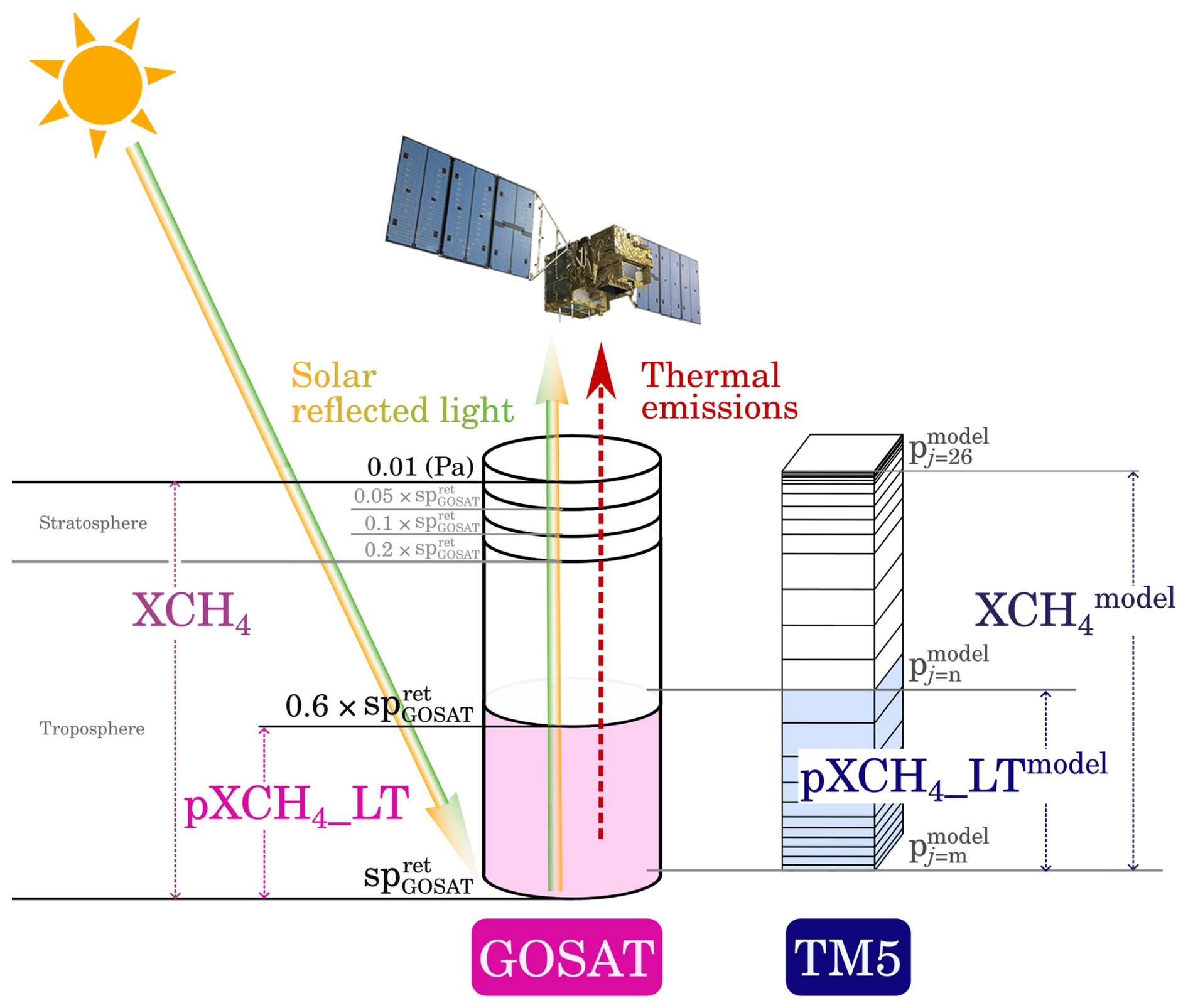
Figure 1 A schematic figure illustrating how total column (XCH₄) and lower-tropospheric partial column (pXCH₄_LT) are calculated in the JAXA/GOSAT data and from TM5. JAXA/GOSAT retrieval algorithm uses information from both solar reflected light and thermal emissions to retrieve partial column CH₄ mole fractions. In JAXA/GOSAT there are five layers between the retrieved pressure (sp${}_{\mathrm{GOSAT}}^{\mathrm{ret}}$) and 0.01 Pa, with two tropospheric and three stratospheric layers. The lower troposphere (LT) is defined as pressure levels between sp${}_{\mathrm{GOSAT}}^{\mathrm{ret}}$ and 0.6 × sp${}_{\mathrm{GOSAT}}^{\mathrm{ret}}$. In TM5, there are 25 model layers, and XCH${}_{\mathrm{4}}^{\mathrm{model}}$ is calculated using all layers, i.e. the pressure levels between $p_{j=\mathrm{0}}^{\mathrm{model}}$ and $p_{j=\mathrm{26}}^{\mathrm{model}}$. For calculation of pXCH₄_LT^model, the minimum level (m) and maximum level (n) vary depending on sp${}_{\mathrm{GOSAT}}^{\mathrm{ret}}$. m=0 if sp${}_{\mathrm{GOSAT}}^{\mathrm{ret}}>p_{\mathrm{j}=\mathrm{0}}^{\mathrm{model}}$ and otherwise the maximum level at which $p_j^{\mathrm{model}}$ exceeds sp${}_{\mathrm{GOSAT}}^{\mathrm{ret}}$. n is the level at which $p_j^{\mathrm{model}}$ reaches 0.6 × sp${}_{\mathrm{GOSAT}}^{\mathrm{ret}}$.

2.3 Atmospheric observations

2.3.1 JAXA/GOSAT partial column data

The JAXA/GOSAT retrieval algorithm is based on the Full Physics algorithm and is extended to use both the 2-orthogonal SWIR and TIR signals simultaneously (Kikuchi et al., 2017). JAXA's forward calculation constructs the vector radiance and uses the two-orthogonal polarized SWIR observation in four windows with bi-directional reflection. For TIR, the scalar radiance is handled in the forward model for three windows. The empirical orthogonal function (EOF) fitting is taken into account in the retrieval process, where XCO₂, XCH₄ and XH₂O are simultaneously retrieved with solar-induced chlorophyll fluorescence (SIF) information. CO₂ and CH₄ partial-column-averaged concentrations are derived for two layers in the troposphere and three layers in the stratosphere. The H₂O concentrations are derived on 11 vertical layers.

The five CO₂ and CH₄ layers are defined by the pressure levels based on the retrieved surface pressure, denoted as sp${}_{\mathrm{GOSAT}}^{\mathrm{ret}}$ (see also Fig. 1). The two tropospheric layers, lower troposphere (LT) and upper troposphere, are defined as the pressure levels between sp${}_{\mathrm{GOSAT}}^{\mathrm{ret}}$ and 0.6 × sp${}_{\mathrm{GOSAT}}^{\mathrm{ret}}$, and between 0.6 × sp${}_{\mathrm{GOSAT}}^{\mathrm{ret}}$ and 0.2 × sp${}_{\mathrm{GOSAT}}^{\mathrm{ret}}$, respectively. The three stratospheric layers are defined as the pressure levels between 0.2 × sp${}_{\mathrm{GOSAT}}^{\mathrm{ret}}$ and 0.1 × sp${}_{\mathrm{GOSAT}}^{\mathrm{ret}}$, between 0.1 × sp${}_{\mathrm{GOSAT}}^{\mathrm{ret}}$ and 0.05 × sp${}_{\mathrm{GOSAT}}^{\mathrm{ret}}$, and between 0.05 × sp${}_{\mathrm{GOSAT}}^{\mathrm{ret}}$ and 0.01 Pa, respectively. In this study, all the GOSAT data are based on the JAXA/GOSAT product v2.0 (https://www.eorc.jaxa.jp/GOSAT/Global_GHGs_Map/index.html, last access: 4 June 2024).

During the study period, the TANSO-FTS and the Cloud and Aerosol Imager (CAI) were shut down, and the observation was suspended during 17–24 May 2018 due to the Command and Data Management System (CDMS) incident and from 24 November until 28 December 2018 due to the rotation anomaly of the second solar paddle.

For comparison to model estimates, the XCH₄ values from model results were calculated as

$$\begin{array}{}\text{(2)}& {\mathrm{XCH}}_{\mathrm{4}}^{\mathrm{model}}={\displaystyle \frac{{\sum }_i({\mathrm{CH}}_{\mathrm{4}i}\times \mathrm{d}{p}_i)}{{\sum }_i\mathrm{d}{p}_i}},i=\mathrm{1},\mathrm{\dots },\mathrm{25},\end{array}$$

where CH_4i is the dry air mixing ratio of CH₄ at TM5 model layer i, temporally and horizontally interpolated to time and location of the JAXA/GOSAT data, and dp_i is the pressure thickness at the layer i.

For calculating modelled lower-tropospheric partial columns of methane, pXCH₄_LT^model, the layers were selected based on sp${}_{\mathrm{GOSAT}}^{\mathrm{ret}}$ (see also Fig. 1). The minimum layer is i=0 if the surface pressure in TM5 model is smaller than sp${}_{\mathrm{GOSAT}}^{\mathrm{ret}}$ and otherwise the maximum layer at which TM5 model pressure exceeds the GOSAT-retrieved surface pressure. The maximum layer corresponded to the point where TM5 pressure reached 0.6 × sp${}_{\mathrm{GOSAT}}^{\mathrm{ret}}$. Vertical interpolation was not applied for simplicity, and therefore, the modelled mixing ratio was calculated using thinner (in case sp${}_{\mathrm{GOSAT}}^{\mathrm{ret}}>$ sp^model) or thicker (in case sp${}_{\mathrm{GOSAT}}^{\mathrm{ret}}<$ sp^model) air mass from the lowest layer. For the uppermost layer, due to the selection method, the model nearly always contained thicker air mass than the retrievals. These likely lead to potential biases (see also Sect. 4.1).

Averaging kernels were not applied to XCH${}_{\mathrm{4}}^{\mathrm{model}}$ and pXCH₄_LT^model, as they were unavailable for the v2.0 product. However, we are aware of a newer version, v3.0 data, where averaging kernels are now available. We did not apply any preprocessing of the JAXA/GOSAT data, such as averaging or removing large-scale differences that may have been raised in comparison to inversion estimates assimilating surface data. This way, we could examine the effect of observations directly. In the assimilation, we assumed observational uncertainty (retrieval error + transport model error) to be (1) 30 ppb globally with a rejection threshold of 60 ppb for both of the XCH₄ or pXCH₄_LT assimilations and (2) 50 ppb with a rejection threshold of 100 ppb in the case that assimilated only pXCH₄_LT data over land (see also Sect. 2.4). The rejection thresholds discriminate the observations if differences between observed and prior-modelled mole fractions exceed the threshold; i.e. the observations are rejected and would not be used to constrain the fluxes. These values are somewhat arbitrary, but they follow other inversion experiments that use the GOSAT data (e.g. Janardanan et al., 2020; Lu et al., 2021; Maasakkers et al., 2021; McNorton et al., 2018). The larger uncertainty is justified as retrieval errors in the lower-tropospheric partial column data are probably higher compared to the total column data.

2.3.2 Surface CH₄ mole fractions

Surface CH₄ mole fraction observations mainly from ObsPack v4.0 (Schuldt et al., 2021) were assimilated in the inversion, as well as used for evaluation (see Fig. A1 for site locations and Table A1 for details). The data include ICOS ATC CH₄ Release and ICOS ATC NRT CH₄ growing time series data, which were downloaded among with other NOAA ObsPack data and the ICOS Carbon portal (Table A2). The data consisted of discrete and continuous observations from in situ stations and ships. Similar to our previous studies (Tsuruta et al., 2017, 2019; Tenkanen et al., 2025), all data were filtered by taking observations at well-mixed conditions based on quality flags given by the data providers. Continuous data were processed into daily means by averaging observations during local time afternoon (12:00–16:00) or night (00:00–04:00). Observational uncertainties (observational error + transport model error) ranged between 4.5–75 ppb, depending on each site (Table A1).

In addition, we used aircraft measurements from the Atmospheric Tomography Mission (ATom; Thompson et al., 2022), obtained from the ObsPack v6.0 (Schuldt et al., 2023) for independent evaluation. During 2016–2019, there were ATom observations from four campaigns: July–August 2016, January–February and September–October 2017, and April–May 2018. Prior and posterior mole fractions were estimated at each sampling location and time, linearly interpolated within the TM5 model grid cells. ATom data were not assimilated in the inversions and therefore can be used as independent observations for validation.

2.3.3 TCCON

The Total Carbon Column Observing Network (TCCON) is a global network providing XCH₄ measurements retrieved from the spectrum of near-infrared radiation of direct sunlight using ground-based Fourier transform spectrometers (FTSs) (Wunch et al., 2011). We used the GGG2020 data (Laughner et al., 2023, 2024) from 25 sites globally (Table A3) for evaluation of inversion results. The sites were selected as those that provided GGG2020 data and have at least 1 year of measurements between 2016–2019. The data were not assimilated in the inversions and so can also be used as independent observations for validation.

For comparison, hourly average mixing ratios interpolated horizontally to the TCCON locations were used. Temporal co-locations were done by selecting the TCCON observations that were closest to the model time step (hourly) and setting the time limit of half an hour; if there was a TCCON observation made within ± half an hour of the model time step, the TCCON and modelled values were taken into account.

For comparison to total column (XCH₄), the model estimates were calculated by applying TCCON averaging kernels (Rodgers and Connor, 2003):

$$\begin{array}{}\text{(3)}& \widehat{c}=c_a+(\mathit{h}\circ \mathit{a}{)}^T(\mathit{x}-{\mathit{x}}_a),\end{array}$$

where $\widehat{c}$ is the averaging-kernel-corrected XCH₄ value from the model, c_a is the TCCON prior XCH₄, h is the TCCON pressure weighting function, a is the TCCON averaging kernel, x is the model profile, and x_a is the TCCON prior profile. After applying the averaging kernel, daily means were calculated for evaluation.

In addition, the tropospheric partial columns were calculated from TCCON total columns of CH₄ and hydrogen fluoride (HF). Practically all of the HF exists in the stratosphere, where HF is produced from photodissociation of chlorofluorocarbons (CFCs). The concentrations of long-lived tracers, such as CH₄ and HF, are strongly correlated in the stratosphere (e.g. Plumb, 2007). Air masses containing both CH₄ and CFCs enter through the topical stratosphere, where CH₄ is oxidized and HF is produced. In the stratosphere, CH₄ shows a nearly linear inverse relationship with HF. By assuming a linear relationship in the stratosphere (Washenfelder et al., 2003; Saad et al., 2014) the tropospheric partial column of ${\mathrm{XCH}}_{\mathrm{4}\mathrm{TCCON}}^{\mathrm{tropo}}$ is given as

$$\begin{array}{}\text{(4)}& {\mathrm{XCH}}_{\mathrm{4}\mathrm{TCCON}}^{\mathrm{tropo}}={\mathrm{XCH}}_{\mathrm{4}}-\mathit{\beta }\times \mathrm{XHF},\end{array}$$

where β is the stratospheric CH₄ : HF slope. As the tracer to tracer correlations typically exhibit distinct correlations in the tropics, extratropics, and polar stratospheric vortices (Plumb, 2007), we derived slopes for the tropics (30° S–30° N), SH (90–30° S), and NH (30–90° N), as well as for the polar stratospheric vortices. Profile data of CH₄ and HF from the Atmospheric Chemistry Experiment – Fourier Transform Spectrometer (ACE-FTS) version 4.1 data products (Boone et al., 2020) were used to calculate the slopes. The polar vortices were identified from potential vorticity data from the ERA5 reanalysis (Hersbach et al., 2020). The vortex edge was assumed to be represented by the $\left|\mathrm{36}\right|$ PVU isoline. The interference of water can increase the error in the column-averaged HF (XHF) (Saad et al., 2014), especially at high air masses. Therefore, observations with column-averaged H₂O (xH₂O) above 2000 ppm and zenith angle larger than $\mathrm{90}-\mathrm{0.0075}\times {\mathrm{xH}}_{\mathrm{2}}\mathrm{O}$ degrees were discarded.

For comparison to the tropospheric partial column, Eq. (2) was applied similarly to calculate pXCH₄_LT^model, but for the lowest and uppermost layer, vertical interpolation was applied to TCCON retrieval surface pressure sp${}_{\mathrm{TCCON}}^{\mathrm{ret}}$ and tropopause height, respectively. The pressure at dynamic tropopause was calculated based on ERA5 reanalysis data, defined by the $\left|\mathrm{2}\right|$ PVU isoline. Constant extrapolation was applied in the case of sp${}_{\mathrm{TCCON}}^{\mathrm{ret}}>$ sp^model.

2.4 Simulation setups

In this study, we present the results from four inversions that differed in the observations assimilated:

• InvSURF – surface CH₄ data only,

• InvGLT – JAXA/GOSAT partial column data (pXCH₄_LT) only,

• InvGLT_land – JAXA/GOSAT partial column data (pXCH₄_LT) over land only,

• InvGTOT – JAXA/GOSAT total column data (XCH₄) only.

In all of the GOSAT inversions, only the JAXA/GOSAT data were assimilated to examine the effect of the data in constraining fluxes independent of other datasets. The inversion without ocean data were tested in consideration of assimilating other satellite data, such as TROPOMI, which do not necessary provide ocean data from all retrieval products. Additionally, considering relatively small contribution of ocean fluxes to global total, compared to that of e.g. CO₂, we examine if land fluxes would be constrained equally well without ocean data.

For InvGLT and InvGTOT, the observational uncertainty and rejection threshold were set to be 30 and 60 ppb, respectively, and for InvGLT_land they were set as 50 and 100 ppb, respectively. All inversions were run for 2015–2019, but 2015 was considered as a spin-up and not included in the analysis. The analysis on regional fluxes was done based on 30° latitudinal bands. Throughout the following sections, the prior and posterior mole fractions refer to those derived using prior and posterior fluxes, respectively.

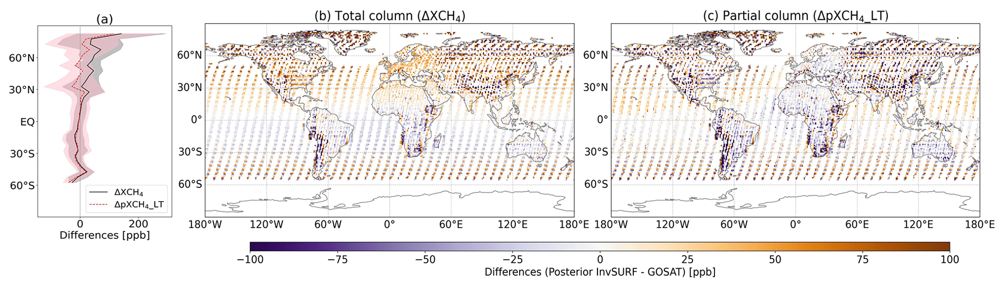
Figure 2 Mean differences between posterior InvSURF and JAXA/GOSAT retrievals, averaged over 2016–2019. (a) 5° latitudinal means (solid line) with standard deviation (shaded area) and (b) and (c) 1°×1° grid means. Positive values indicate posterior InvSURF mole fractions being higher than the JAXA/GOSAT retrievals.

3 Results

3.1 Comparison of CH₄ mole fractions from InvSURF and JAXA/GOSAT

In this section, we analyse the differences between posterior estimates from the surface-based inversion (InvSURF) and JAXA/GOSAT retrievals for total and partial columns, i.e.

$$\begin{array}{}\text{(5)}& \begin{array}{rl}& \mathrm{\Delta }{\mathrm{XCH}}_{\mathrm{4}}={\mathrm{XCH}}_{\mathrm{4}\mathrm{InvSURF}}^{\mathrm{post}}-{\mathrm{XCH}}_{\mathrm{4}\mathrm{GOSAT}}^{\mathrm{ret}}\\ & \mathrm{\Delta }{\mathrm{pXCH}}_{\mathrm{4}}\mathrm{\_}\mathrm{LT}={\mathrm{pXCH}}_{\mathrm{4}}\mathrm{\_}{\mathrm{LT}}_{\mathrm{InvSURF}}^{\mathrm{post}}-{\mathrm{pXCH}}_{\mathrm{4}}\mathrm{\_}{\mathrm{LT}}_{\mathrm{GOSAT}}^{\mathrm{ret}}.\end{array}\end{array}$$

In the comparison of total column, latitudinal biases were found with positive ΔXCH₄ values in the extratropics and negative values in the tropics, especially in the SH tropics (Fig. 2b). This feature was systematic in time, such that similar biases were found regardless of years and seasons, although the absolute value of the biases varied. In the comparison of lower-tropospheric partial columns, such latitudinal biases were less prominent (Fig. 2c), especially over land, indicating better agreement over NH extratropics (Fig. 2a). This indicates the potential role of upper atmosphere in the total column biases, where posterior estimates and retrievals had difficulty agreeing.

Large biases were observed in regions such as Greenland, western South America, southernmost South Africa, eastern China, and northern Russia in both comparisons (Fig. 2b and c). Because of the challenges in retrieving data over ice-covered land, we assume that biases in Greenland were mostly associated with retrieval errors. Biases in other regions could be due to unresolved fluxes by surface observations, i.e. the inversion error in estimating fluxes, retrieval errors due to cloud cover, and difficulties in retrieving surface pressure in regions with highly elevated surface. The horizontal resolutions of the transport model also contribute to the biases in highly elevated areas. The additional simulation with TM5 showed that increasing resolution from 4°×6° (latitude × longitude) to 2°×3° decreased biases in mountain regions in Africa and the Tibetan Plateau, although the biases in regions such as the Andes mountains in South America and the edges of the Tibetan Plateau still remain (Fig. A2). We also acknowledge that the vertical interpolation and averaging kernel (AK) contribute to the biases in highly elevated areas, especially for XCH₄ (Fig. A3) (see also Sect. 4.1).

Europe showed the smallest ΔpXCH₄_LT, which is encouraging considering that InvSURF probably had constrained the emission in Europe the best compared to other regions globally, and modelled tropospheric CH₄ from InvSURF is well in line with ground-based observations (Sect. 3.2). Both the transport model and optimization resolutions were the smallest and number of observations were relatively large in Europe (Sect. 2.1). There was a notable shift between better agreement in Europe and a worse agreement in Russia and Africa, attributed to the CTE-CH₄ setup: TM5 was run with highest spatial resolution over Europe and an extended area (Tsuruta et al., 2015), with a coarser resolution elsewhere. This resulted to creating an artefact of a border between the zoom grid and the global grid that caused the shift. An additional simulation with TM5 with global 2°×3° (latitude × longitude) resolution and without zoom eliminated these boundaries (Fig. A2).

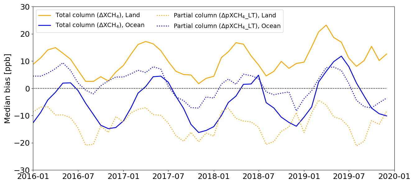
Figure 3 Global monthly median differences between posterior InvSURF and JAXA/GOSAT retrievals. Positive values indicate posterior InvSURF mole fractions being higher than the JAXA/GOSAT retrievals.

Both lower-tropospheric partial and total column comparisons showed seasonal and land–sea biases (Fig. 3). The global averages of ΔXCH₄ and ΔpXCH₄_LT were smaller during NH autumn–winter than spring–summer. The amplitude of the seasonal biases was larger in the total column, especially over the oceans. The comparison of the land and sea biases showed that the biases in the total column were larger over land than ocean, whereas an opposite behaviour was observed for the lower-tropospheric partial columns. In other words, the ΔXCH₄ and ΔpXCH₄_LT were closer over the ocean than land on average, with absolute median monthly differences of 5 ppb over the ocean and 23 ppb over land, indicating the possible influence of land fluxes to upper atmosphere. Overall, the average bias during 2016–2019 was smallest in ΔpXCH₄_LT over the ocean.

3.2 Evaluation against surface and aircraft data

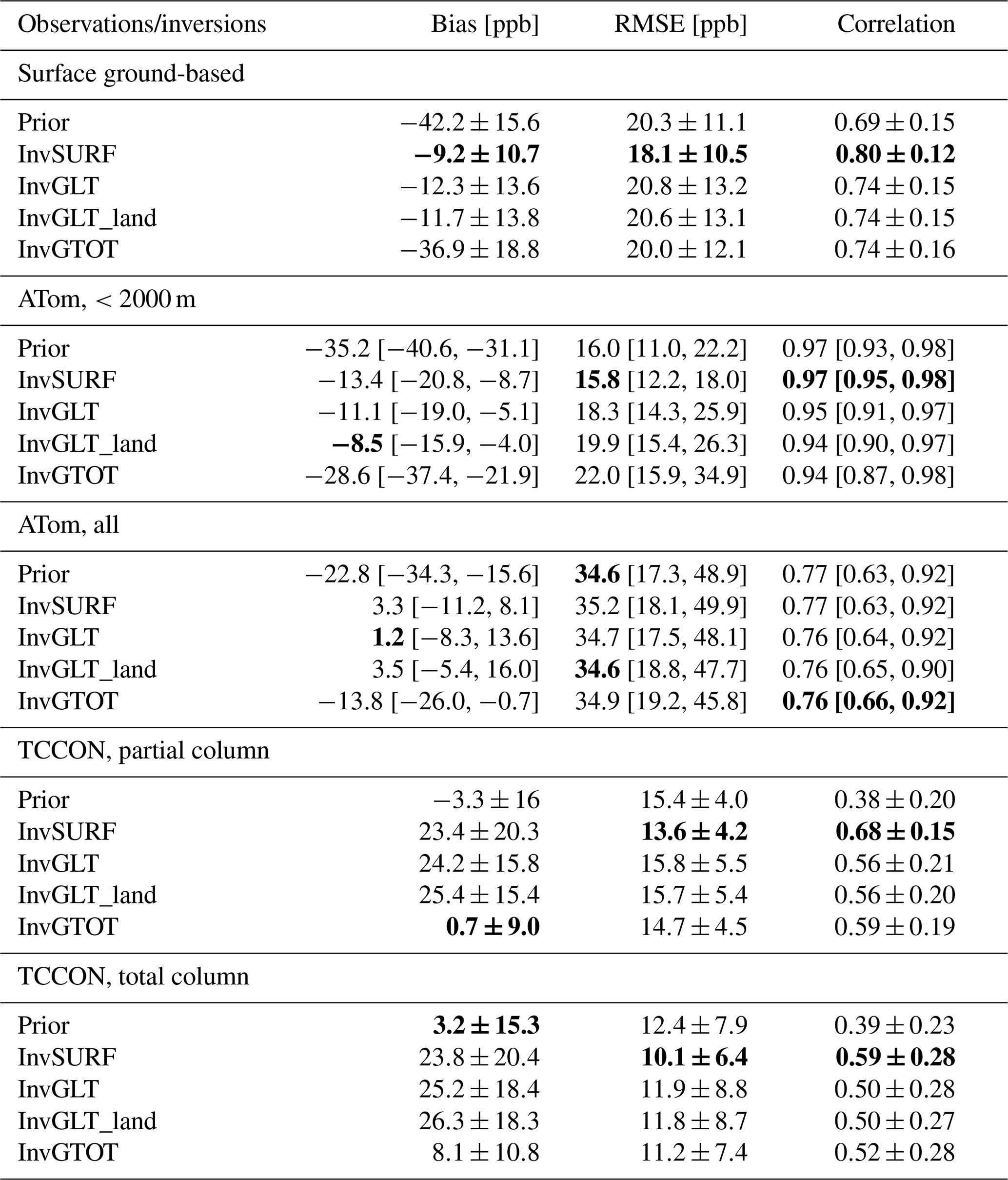
Comparison of posterior atmospheric CH₄ to the surface ground-based observations showed the smallest overall bias, root mean squared error (RMSE), and strongest correlation for InvSURF (Table 1) as expected, since these observations were assimilated in the inversion. Among the GOSAT inversions, those using the lower-tropospheric partial column data (InvGLT and InvGLT_land) showed the best agreement to the surface ground-based observations, while the total column inversion (InvGTOT) showed large negative biases following the prior (Table 1). RMSE and correlation within the GOSAT inversions were not significantly different. The latitudinal gradient was best captured by InvSURF, InvGLT, and InvGLT_land compared to the surface stations (Fig. 4a). The inversions mostly underestimated the surface observations with the underestimation being the smallest in the Southern Hemisphere (SH) for InvGLT and InvGLT_land and in the Northern Hemisphere (NH) for InvSURF. InvGTOT showed better agreement than InvSURF in the SH but considerable underestimation in the NH (Fig. 4a), which was the reason for strong negative bias in the overall agreement (Table 1).

In the mid-latitudes and high northern latitudes (above 30° N) the seasonal cycle amplitude (SCA) was generally overestimated by model estimates in the prior inversion, which was worsened by inversion (SCA of posterior estimates were larger than prior) (Fig. A4). In addition, seasonal minima in the NH occurred 1 to 2 months later than observations, although the results in InvSURF were slightly better than in the prior and GOSAT inversions (Fig. A4). This indicates either possible errors in seasonal cycles of posterior emission or atmospheric chemical sinks.

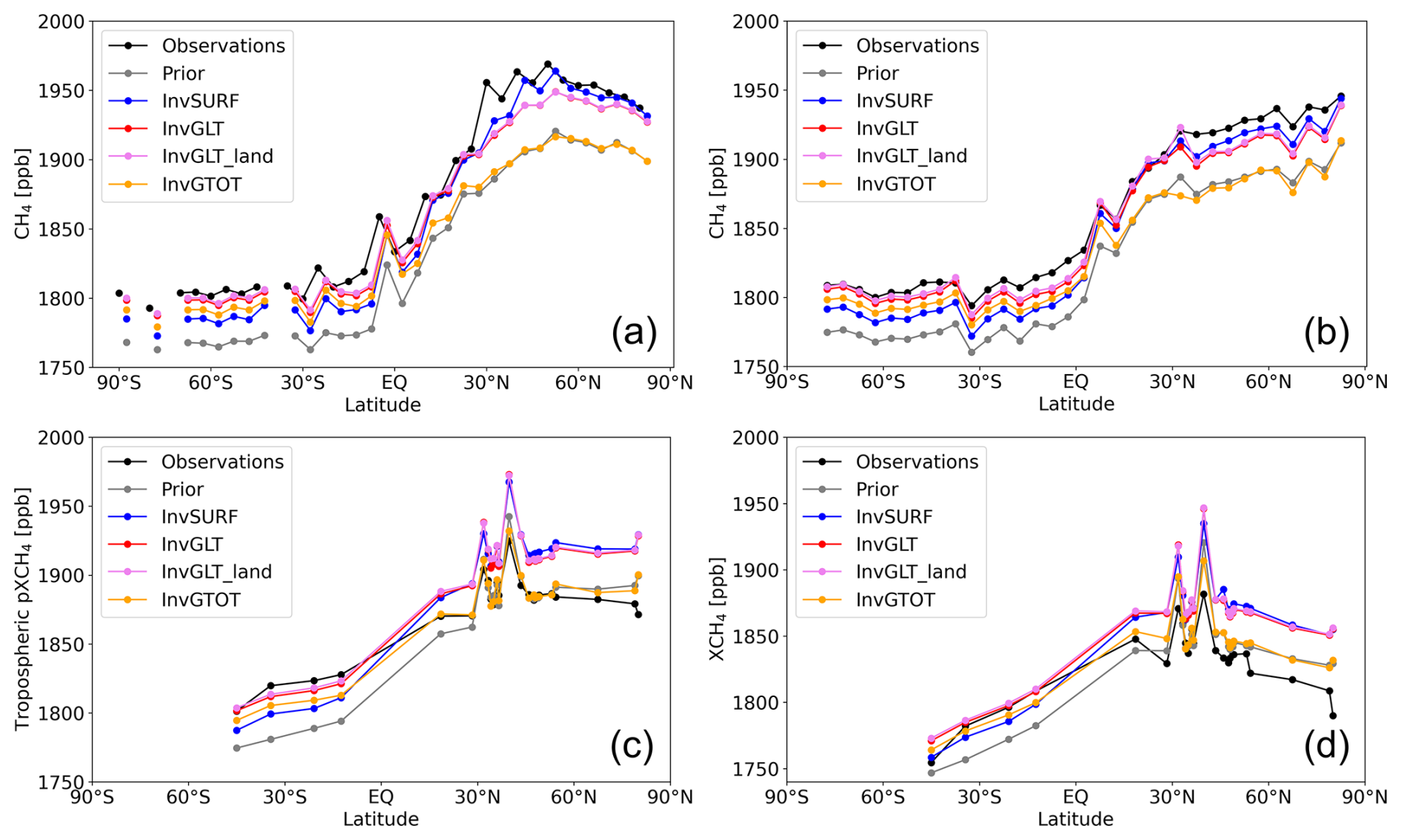
Figure 4 Mean atmospheric CH₄, averaged over 2016–2019 at (a) surface ground-based and shipboard stations, (b) ATom observation locations at the altitude band 0–2000 m, and (c) and (d) TCCON sites. Panel (c) shows comparison of tropospheric partial column and (d) total column. For (a), the data that were assimilated in InvSURF were used. For (a) and (b), means over 5° latitude bands are shown. For (c) and (d), no spatial averaging is applied. The coloured lines are the posterior estimates from each inversion, which is estimated by running TM5 forward using posterior fluxes of the corresponding inversion simulation.

Comparison to ATom aircraft data also showed that on average, InvSURF, InvGLT, and InvGLT_land resulted in the best statistics (Table 1), and the latitudinal gradient agreed better with the observations compared to InvGTOT at the altitude bands 0–2000 and 2000–4000 m above sea level ($\mathrm{m}\mathrm{a}.\mathrm{s}.\mathrm{l}.$) (Figs. 4b, A5 and A6). In these altitude zones, the mean bias was significantly larger in InvGTOT, which was in line with the results compared to surface ground-based stations (Table 1). This height corresponds approximately to the height where most of the surface ground-based stations were situated and from which JAXA/GOSAT XCH₄_LT data were calculated. Between 4000–8000 $\mathrm{m}\mathrm{a}.\mathrm{s}.\mathrm{l}.$, the latitudinal gradients from InvGTOT were better captured, whereas the other inversions overestimated these gradients (Fig. A6). Considering that the tropopause height is around 9000 $\mathrm{m}\mathrm{a}.\mathrm{s}.\mathrm{l}.$ or above, these results indicate that the transport model has problems in representing upper-tropospheric concentrations. This is consistent with the finding that all model estimates worsened at high altitudes (>8000 $\mathrm{m}\mathrm{a}.\mathrm{s}.\mathrm{l}.$). All model estimates, both prior and posterior, failed to capture low mole fractions observed in high-latitude (>50° N/S) regions (Fig. A5). Such low CH₄ mole fractions were observed especially in the winter of 2017 and the spring of 2018 when the tropopause height was lower and the ATom aircraft operated in the stratosphere (Fig. A7). This is when the disagreement was strongest, possibly indicating the improper modelling of vertical profiles in polar vortex conditions.

Table 1 Bias, root mean squared error (RSME), and Pearson's correlation against observations at surface ground-based stations assimilated in InvSURF, ATom aircraft measurements, and TCCON data. The statistics were calculated for each ground-based and TCCON station over 2016–2019 and four ATom campaigns separately, and the mean of all stations or campaigns is shown. The value followed by ± sign is the standard deviation (std) of statistics from all stations. For ATom, the minima and maxima of the statistics are shown in square brackets instead of std due to the limited number of campaigns (four) to calculate std from. Biases were calculated as modelled values subtracted by observed values, and therefore, positive values indicate model overestimation. The simulations with the best statistics are highlighted in bold.

3.3 Evaluation against TCCON

The latitudinal gradient was generally weaker in TCCON tropospheric partial and total columns (Fig. 4) compared to the surface observations, indicating the smaller influence of surface fluxes. Therefore, the evaluation against the TCCON data provides limited information about how well the inversions constrained the surface fluxes but focuses more on the model performance regarding long-range transport, tropopause mixing and atmospheric chemistry, which are important to take into account when assimilating total column satellite data. In the northern high latitudes, the extracted TCCON partial columns successfully separated the stratospheric component, showing no significant low biases under polar vortex conditions (Fig. A8).

Compared to the surface data comparison, the TCCON comparison showed better overall agreement and improved representation of the latitudinal gradient in InvGTOT compared to other inversions for both total and tropospheric partial columns (Table 1, Fig. 4c and d). In the NH, all model estimates exhibited overestimation, driven by larger latitudinal gradients, with InvSURF, InvGLT, and InvGLT_land performing worse than InvGTOT. Considering also that InvGTOT showed the best agreement with the comparison to Atom data between 4000–8000 $\mathrm{m}\mathrm{a}.\mathrm{s}.\mathrm{l}.$ on latitudinal gradients, this indicates the importance of the upper troposphere in the estimation of XCH₄. This finding also denotes that model biases in the estimation of XCH₄ are not solely caused by errors in resolving stratospheric concentrations; the errors in the upper troposphere also contribute to total column biases.

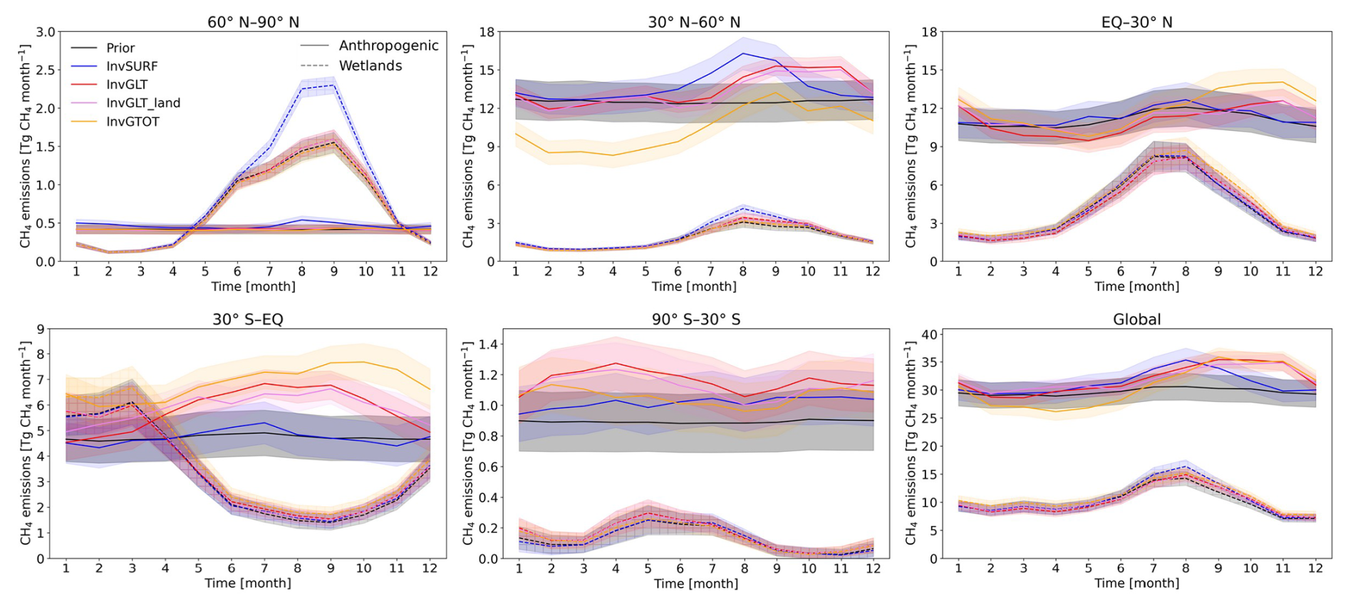
Figure 5 Monthly mean anthropogenic and wetland CH₄ emissions at 30° latitudinal bands and global totals. The means are taken from 2016–2019. Shaded areas illustrate uncertainty as standard deviations of 500 ensemble members.

Table 2 Global and regional CH₄ emissions (Tg CH₄ yr⁻¹), averaged over 2016–2019. Uncertainty presented in numbers after ± sign is the standard deviation of 500 ensemble members in CTE-CH₄.

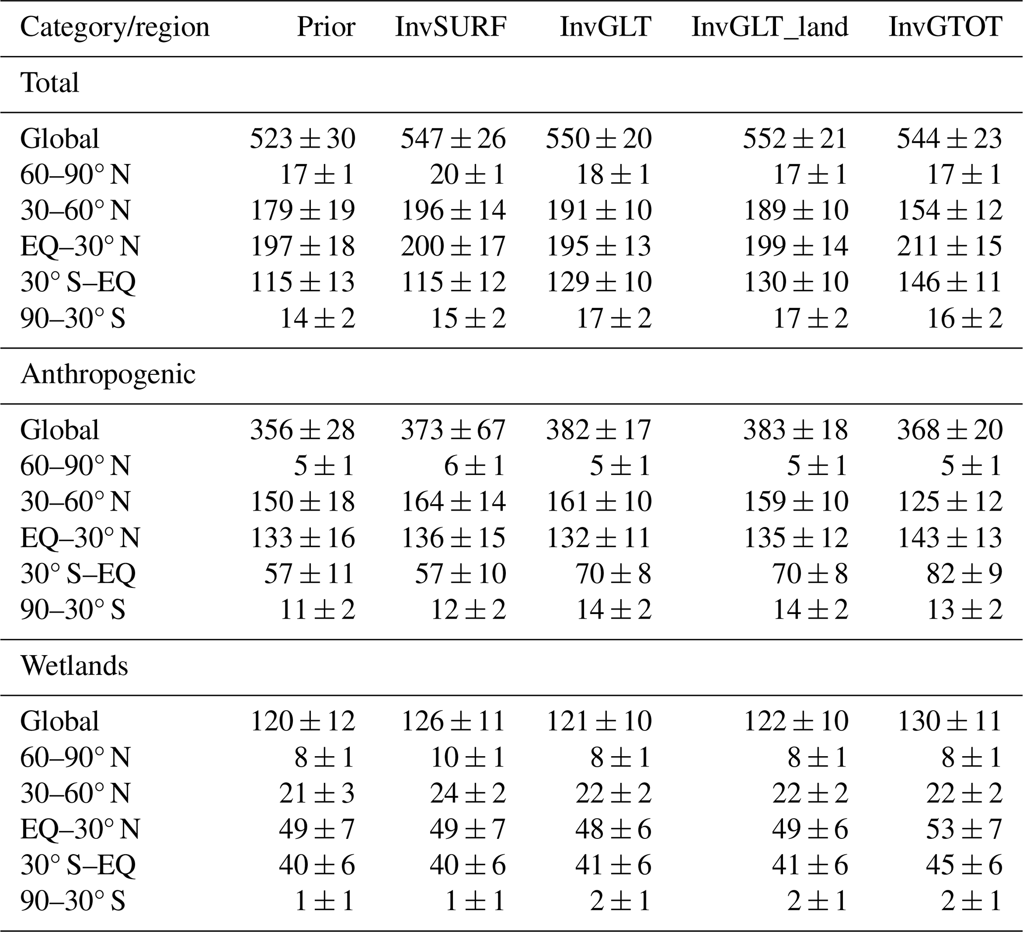
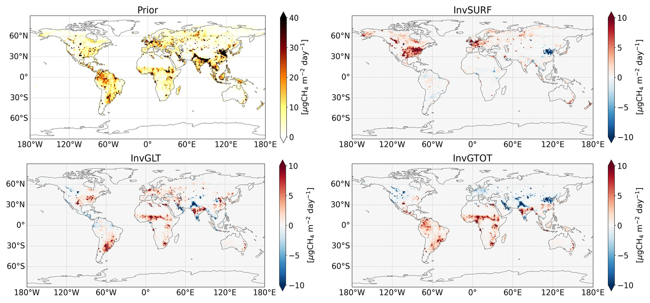
Figure 6 Prior total CH₄ emissions (left top) and emission increments (posterior – prior), averaged over 2016–2019. Positive values indicate posterior emissions being higher than the prior.

3.4 CH₄ fluxes

The 2016–2019 average global total and regional (30° latitudinal band) emissions are presented in Table 2. The posterior global total emissions were similar in all inversions (544–552±20–26 Tg CH₄ yr⁻¹) and showed increases from the prior with reduction in uncertainty (523±30 Tg CH₄ yr⁻¹). Most of the increase from the prior was attributed to anthropogenic emissions (c.a. 57 %–96 %). The sectorial emissions showed that anthropogenic emissions were higher and wetland emissions lower in InvGLT and InvGLT_land compared to InvSURF and InvGTOT. The anthropogenic emissions in the SH in InvGLT and InvGLT_land were higher compared to InvSURF but comparable in magnitude to InvSURF in the NH. InvGTOT also showed higher anthropogenic emissions in the SH compared to InvSURF, especially in the tropics (30° S–EQ), but lower anthropogenic emissions in 30–60° N.

Between the tropics and SH (90° S–30° N), the posterior anthropogenic emissions in the GOSAT inversions deviated more from the prior compared to InvSURF (Table 2, Fig. 5). This difference was primarily associated with emissions over South America, Africa, and India (Fig. 6). The monthly variations of anthropogenic emissions deviated largely from the prior in the GOSAT inversions (Fig. 5). All GOSAT inversions showed an emission peak in November in the region from the Equator to 30° N, which was 3 months later than prior and InvSURF. In 30° S–EQ, all GOSAT inversions showed a clear seasonal cycle with emissions peaking during April–November. In contrast, the prior had no clear seasonal cycle, and InvSURF showed a small seasonal cycle with a peak in July. In 90–30° S, InvGLT and InvGLT_land showed two emission peaks, one around April and another in October. InvGTOT did not show the April peak, but it aligned with InvGLT and InvGLT_land in presenting an emission reduction in August and peak in October. InvSURF showed a less distinct seasonal cycle with emissions constantly increasing from the prior in all months, except January. In the tropics, there are only a few surface stations (Fig. A1), which are often far from emission sources, measuring background mixing air. As a result, the JAXA/GOSAT data likely contained more valuable information to constrain the fluxes in these regions compared to the sparse surface data.

In 30–60° N, posterior anthropogenic emissions in InvGTOT were about 35 Tg CH₄ yr⁻¹ lower than those in the other inversions (Table 2), representing about 6 % of the global total. These differences were not associated specifically with a specific region, but InvGTOT showed mostly negative emission increments indicating that posterior emissions were lower than the prior in this region (Fig. 6). Unlike the tropics, there are a relatively large number of surface stations in Europe and the best optimization setup in terms of model spatial resolution, and thus, we suspect that the results from InvGTOT in Europe may have been too low. The comparison to ground-based observations in Europe also showed strong underestimation in InvGTOT (−44 ppb on average compared to stations within the 34–73° N, 12° W–37° E domain). For other regions, considering that the regions such as USA and China are large CH₄ emitters (Petrescu et al., 2024), we also suspect that the results in InvGTOT were underestimated, possibly due to the ability of the transport model representation of XCH₄ (see also Sect. 4.2).

In 60–90° N, posterior wetland emissions in the GOSAT inversions stayed close to the prior compared to InvSURF (Table 2). While InvSURF showed an increase in summer wetland emissions, such change was not found in the GOSAT inversions. Therefore, the seasonal cycle amplitude of wetland emissions was smaller in the GOSAT inversions (Fig. 5). It is known that the GOSAT data have sampling limitation during winter due to polar nights and very low solar zenith angles. However, JAXA/GOSAT data were available above 60° N during summer (Fig. 2). Further, as we found from the comparison of JAXA/GOSAT retrievals to InvSURF (see Sect. 3.1), posterior mole fractions in InvSURF were higher than the JAXA/GOSAT retrievals, indicating that emissions from the GOSAT inversions would likely be lower than those from InvSURF. Therefore, we argue that the lower emissions from the GOSAT inversions were not due to limited number of data but rather reflected the agreement between the inversion and the prior. However, the inversion setups, such as the observation and transport model biases and uncertainties, rejection threshold and prior emission uncertainty, may need to be investigated further to better constrain the fluxes using the satellite data.

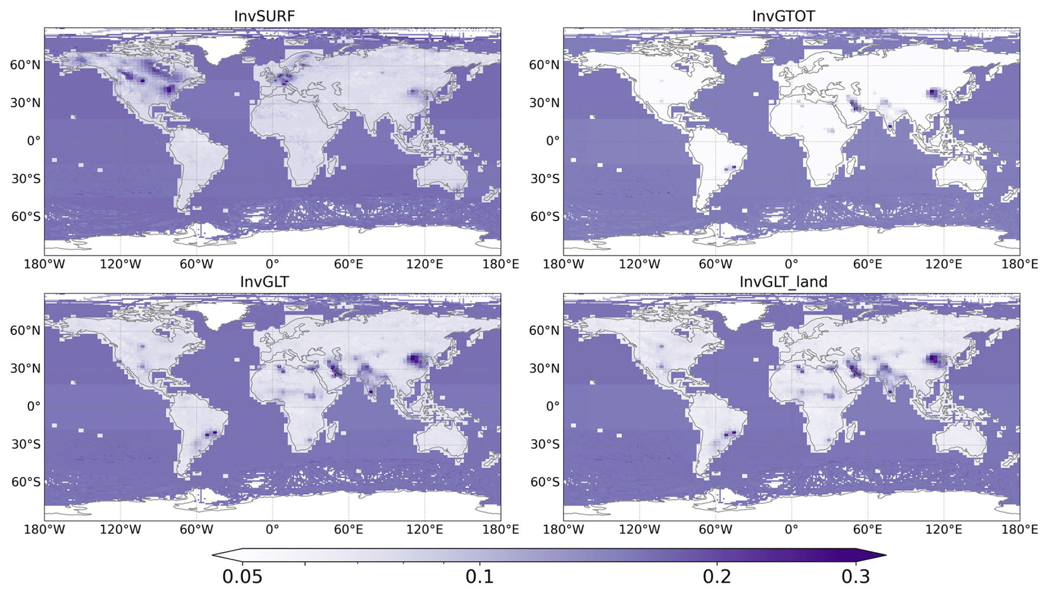
Figure 7 Annual mean uncertainty reduction rate $({\mathit{\sigma }}_{\mathrm{prior}}-{\mathit{\sigma }}_{\mathrm{posterior}})/{\mathit{\sigma }}_{\mathrm{prior}}$ of total fluxes, averaged over 2016–2019. σ values were calculated as standard deviation from 500 ensemble members. Note the colour is on a logarithmic scale.

3.5 Uncertainty estimates

Despite a rather arbitrary choice of prior observational uncertainty (diagonals of R in Eq. 1; see Sect. 2.1 and 2.3), the posterior emission uncertainties were generally lower in the GOSAT inversions compared to InvSURF, and lowest in InvGLT. These differences were most pronounced in the NH tropics (EQ–30° N) (Table 2). The differences between InvSURF and GOSAT inversions were probably driven by the number of available observations, since GOSAT had much more data in the tropics. This could also explain in part the latitudinal bias found in Sect. 3.1. Within the GOSAT inversions, the number of assimilated data was higher in InvGTOT than InvGLT (Fig. A9), even though the observational uncertainty and rejection thresholds were the same in both inversions. This indicates that the lower uncertainty in InvGLT was not simply due to number of assimilated observations but also related to sensitivity of the data to surface fluxes. Due to the nature of the retrieved quantity, total columns have less sensitivity to surface fluxes than ground-based data or lower-tropospheric partial column data; i.e. the total column data would have less power to constrain surface fluxes. Therefore, the larger number of assimilated observations in InvGTOT did not necessary lead to higher uncertainty reduction rates than in InvGLT. However, it is possible that the prior observational uncertainty prescribed in InvGLT may have been underestimated, considering that retrieval errors are probably higher for lower-tropospheric partial columns compared to total columns. Consequently, the posterior uncertainty of the fluxes may have been also underestimated. On the other hand, the transport model error may be lower for the lower-tropospheric partial column data, considering that the transport model performs better in representing tropospheric concentrations than stratospheric, so the total observational uncertainty could have been reasonable. The global total flux uncertainty of InvGLT_land was slightly higher compared to InvGLT. The posterior uncertainty was higher in the region with the largest uncertainty (EQ–30° N). Since the flux horizontal and seasonal distributions in InvGLT_land did not change significantly from InvGLT overall, we could argue that the effect of ocean data as a constraint was minor.

The spatial distribution of uncertainty reduction rates is shown in Fig. 7. This figure indicates that the GOSAT inversions constrained fluxes mostly in tropical regions and northeast China, while InvSURF showed strongest reductions in the USA, Canada, and Europe. InvSURF also showed a reduction hotspot areas in northeast China, but the signal was much weaker compared to the GOSAT inversions. The uncertainty reduction rates over land in InvGTOT were weak in general, with fewer reduction in hotspots compared to InvGLT and InvGLT_land, indicating that the use of the lower-tropospheric partial column data was more effective in constraining fluxes compared to total column data. The inversions with lower-tropospheric partial column data showed stronger uncertainty reduction rates in Africa and India, which were not as prominent in other inversions. The weaker uncertainty reduction rates from the GOSAT inversions in North America and Europe were probably due to (1) larger uncertainty in the observations, where many surface observations in these regions had less than 30 ppb observation uncertainty (Table A1), and (2) the lack of observations in high latitudes over winter.

The uncertainty reduction rates over the ocean were relatively large compared to those over land (Fig. 7). This is mainly due to the assigned prior uncertainty, which was significantly smaller over the ocean; the emissions were low (Fig. 6), and prior uncertainty was set to 20 % over the ocean (see Sect. 2.1). This has led to prior uncertainty of $\sim {\mathrm{10}}^{-\mathrm{22}}$ mol m⁻² s⁻¹ over the ocean, which is approximately 10¹² smaller than those over land. The uncertainty reduction rates are sensitive to small changes when the prior uncertainties are small, and therefore, they became larger over the ocean, although the absolute changes in the uncertainties were small.

4 Discussion

4.1 Effect of vertical interpolation and averaging kernels

In this study, we did not apply vertical interpolation for simplicity or averaging kernels (AKs) as JAXA/GOSAT v2.0 did not provide the information. However, we acknowledge that these are important to take into account when possible. With test simulations with TM5, we found that the latitudinal biases improved in ΔXCH₄ when compared to JAXA/GOSAT v3.0 data with vertical interpolation and AKs applied (Fig. A3). In the NH temperate regions, the biases in ΔXCH₄ turned from positive to negative and became similar to the biases in the tropics. Therefore, using v3.0 would possibly increase the CH₄ flux estimates from the NH temperate regions in InvGTOT, aligning better with the inversions using surface and lower-tropospheric partial column data. There are still positive biases in the high latitudes, although they are smaller than these compared to v2.0 data without interpolation and AK.

For the lower-tropospheric partial column, ΔpXCH₄_LT, the overall latitudinal biases did not change significantly by applying vertical interpolation and AK (Fig. A3). However, the large positive biases in highly elevated regions (e.g. Andean region in South America and the Tibetan Plateau in China and surroundings) and the northeastern part of China, where CH₄ emissions are large, turned to large negative biases. Nevertheless, large biases, both positive and negative, mean that the observations are likely to be rejected during assimilation and would not affect flux estimates. The ΔpXCH₄_LT over the ocean showed less latitudinal bias – the negative biases in the SH tropics turned positive. Overall, the robustness of modelling the lower-tropospheric partial column could be considered an advantage over the total column, having potential to provide more robust estimates regardless of differences in how transport models represent long-range transport, tropopause mixing, and atmospheric chemistry.

4.2 Role of upper atmosphere and OH in the estimation of XCH₄ values

Latitudinal differences between posterior from the surface inversion and satellite total column retrievals have been seen in earlier studies using TM5 and other global Eulerian atmospheric chemistry transport models (Alexe et al., 2015; Qu et al., 2021; Tsuruta et al., 2017; Turner et al., 2015; Zhang et al., 2021). Such discrepancies were reported regardless of the satellites' retrieval products, prior fluxes, years, or seasons. Part of the misrepresentation of CH₄ mole fractions in the upper troposphere could be due to convection schemes in the transport models (Saito et al., 2013), but the exact effect on the representation of total column values is to be examined. In high northern latitudes, the stratospheric profile is one of the challenges, especially in polar vortex conditions (Tsuruta et al., 2023). However, polar vortex occurs only occasionally in spring, and our comparison to GOSAT, TROPOMI and TCCON XCH₄ values in this and previous studies showed biases even during the periods without polar vortex conditions (Tsuruta et al., 2017, 2023). As shown in this study, latitudinal biases occur already in the upper troposphere (Fig. A6), which confirms the findings from Lindqvist et al. (2024), who argued that the role of the stratosphere in the estimation of XCH₄ was minor.

In addition, we found that using higher horizontal resolution in TM5 improves agreement in the lower-tropospheric partial and total columns (Fig. A2), indicating the importance of the transport model resolution. The latitudinal biases indeed seem to be slightly lower using higher spatial resolution (Stanevich et al., 2021), although the exact effect is to be examined. This study was limited in its exploration of the impact of the horizontal resolution, but increasing model resolution in the vertical dimension could also improve the representation of upper atmospheric CH₄.

The discrepancies in the latitudinal gradient could also be caused by the choice of chemistry schemes in the transport models. The distribution of OH, the largest sink of CH₄ (Saunois et al., 2025), plays an important role in regulating ambient methane levels. The OH concentration fields by Spivakovsky et al. (2000) used in this study and several others (Patra et al., 2011; Saunois et al., 2025) have relatively uniform inter-hemispheric distributions, possibly underestimating the OH concentration in the NH and overestimating them in the SH (Zhao et al., 2019). This leads to higher atmospheric CH₄ in the NH and lower atmospheric CH₄ in the SH, as shown by this study and previous studies (Tsuruta et al., 2017, 2023). Zhao et al. (2020) showed that the differences in the inter-hemispheric distribution of OH could lead to about 25–50 Tg CH₄ yr⁻¹ differences in the inter-hemispheric distribution of CH₄ emissions, where the inversion based on Spivakovsky et al. (2000) led to lower emissions in the NH and higher emissions in the SH. This outcome is in line with the conclusion that the emission distributions in InvGTOT, which estimated the lowest CH₄ emissions in the NH, could be unreliable. The vertical OH profiles used in this study that have distinct peaks at around 500–600 hPa (Zhao et al., 2019) may also partially explain why ATom profiles and GOSAT total columns were not accurately reproduced.

4.3 Land–sea discrepancies

In CH₄ inversions using the GOSAT data, it has not been common to correct land–sea biases in the retrievals or exclude data over the ocean. CH₄ fluxes over the ocean are minor compared to those over land (Saunois et al., 2025). Consequently, the effect of land–sea biases in the JAXA/GOSAT retrieval data is expected to be small in estimation of CH₄ fluxes. This study showed that the emission estimates and posterior mole fractions from InvGLT and InvGLT_land were very similar, despite the different systematic and seasonal biases over land and sea compared to InvSURF (Fig. 3), confirming that the effect of ocean data as constraints has a minimum influence on the outcome of inversions. Therefore, to significantly decrease the number of data in the inversions and increase the computational efficiency.

4.4 Global and regional emissions

The global total estimates from InvSURF were slightly lower than from the inversions using JAXA/GOSAT_LT data and on the lower edge of the range of the top-down (TD) estimates from the latest Global Methane Budget (553–586 Tg CH₄ yr⁻¹, 2010–2019 average; Saunois et al., 2025). The breakdown of anthropogenic and wetlands sources showed that anthropogenic emissions from this study were slightly higher compared to Saunois et al. (2025) (350–391 Tg CH₄ yr⁻¹ vs 145–214 Tg CH₄ yr⁻¹, 2010–2019 TD averages). These differences occur probably because of smaller wetland prior emissions (120 Tg CH₄ yr⁻¹), which are on the lower boundary of bottom-up estimates from Saunois et al. (2025) (119–203 Tg CH₄ yr⁻¹, 2010–2019 bottom-up averages). This indicates that the prior uncertainty may need to be revised, and for example, spatially and seasonally varying uncertainty ratios (Tenkanen et al., 2025) could provide better freedom in the inversion. It is worth pointing out that we did not use a separate prior for freshwater emissions, and, thus, the freshwater emissions could be wrongly attributed to anthropogenic emissions if there is a spatial overlap with the anthropogenic emissions.

The total emissions in the eastern part of North America agree well with previous studies (Alexe et al., 2015; Baray et al., 2021; Lu et al., 2022). Higher emissions in the northeastern part of the United States compared to EDGAR (Fig. 6) point to underestimation of emissions from oil and gas. It should be noted that although we used the newer version of EDGAR (v8.0) in this study, the underestimation still seems to remain. The seasonal variability of anthropogenic CH₄ emissions in southern North America (including the contiguous United States and Mexico) from the GOSAT inversions (Fig. A10a) showed opposite patterns compared to InvSURF. The seasonal cycle in this region is likely to be associated with natural gas consumption (Zeng et al., 2023) and agriculture (Maasakkers et al., 2023). In contrast to results from Maasakkers et al. (2023), who argue that the seasonal pattern of natural gas consumption has strong interannual variations and is spatially inhomogeneous, our results from the GOSAT inversions were similar to those from Miller et al. (2013), which showed larger emissions during autumn and winter compared to summer.

In China, InvSURF and InvGTOT showed strong negative emission increments (i.e. posterior emissions were lower then prior) around Beijing (Fig. 6), which is consistent with studies such as by Lu et al. (2021) and Wang et al. (2022), who assimilated both surface and the GOSAT XCH₄ data. This seems to be a common feature found in other studies despite different GOSAT retrieval products, prior, transport, and inverse models being used (Lu et al., 2021, and references therein). On the other hand, InvGLT and InvGLT_land showed positive emission increments in eastern and southern China. This is closer to the findings from Chen et al. (2022), who assimilated the TROPOMI XCH₄ data. However, these results again contradict with Qu et al. (2021) who assimilated both GOSAT and TROPOMI XCH₄ data and argued that an inversion using only TROPOMI XCH₄ may be unreliable over China because the TROPOMI XCH₄ is strongly affected by cloud cover.

In central Africa and South Sudan wetland regions, our GOSAT inversions showed a large increase in total emissions (Fig. 6), which were primarily associated with wetland emissions. This is in line with findings from Lunt et al. (2019), who used the GOSAT XCH₄, and Pandey et al. (2021), who used the TROPOMI XCH₄ in their inversions, although our posterior estimates were considerably lower. For instance, we found monthly maxima below 1 Tg CH₄ per month around South Sudan, compared to Lunt et al. (2019) estimates of 7 Tg CH₄ per month and Pandey et al. (2021) estimates of seasonal cycle amplitude of about 2–3 Tg CH₄ per month. Nevertheless, the seasonal cycle in this region from the GOSAT inversions (Fig. A10b) showed significantly lower emissions in June–July and later maxima in August–September compared to prior and InvSURF. This corresponds slightly better to dry and wet seasons and is in line with Lunt et al. (2019) and Pandey et al. (2021), although we could not reproduce high emissions in late months.

The magnitude of high-northern-latitude (NHL) wetlands remained uncertain. Previous studies showed that in some cases, NHL emissions from the inversion based on the GOSAT data were lower compared to those based on surface data (Pandey et al., 2016; Feng et al., 2017), while others showed the opposite (Alexe et al., 2015; Baray et al., 2021). Our analysis showed that the wetland emissions for 60–90° N were lower in the GOSAT inversions regardless of the assimilated data type (total or lower-tropospheric partial column) compared to InvSURF. This is in line with our previous studies assimilating TROPOMI XCH₄ data (Tsuruta et al., 2023) and using other wetland priors, such as JSBACH-HIMMELI, where emissions were relatively larger among process-based models (Aalto et al., 2025; Tenkanen et al., 2025). Tsuruta et al. (2023) assumed that the lower NHL wetland emissions in the TROPOMI inversions were due to latitudinal biases associated with model–retrieval differences (Lindqvist et al., 2024). However, as shown in this study, the inversion using lower-tropospheric partial column data also resulted in lower NHL wetland emissions compared to InvSURF, indicating that there may be fundamental discrepancies between satellite and surface inversions. The differences were partly due to spatial coverages and temporal distributions of the observations and uncertainties associated with transport models, observations, prior emissions and possible biases in the satellite data, but further study is needed to find the exact cause of these discrepancies and to obtain more robust the emission estimates.

5 Conclusions

This study presented the advantages of JAXA/GOSAT lower-tropospheric partial column retrievals in estimating global and regional CH₄ budgets using the CTE-CH₄ atmospheric inverse model. Our findings showed that assimilating the lower-tropospheric partial column data led to posterior CH₄ fluxes and atmospheric CH₄ mole fractions that were more consistent with the inversion estimates using surface data compared to total column retrievals. In addition, partial column retrievals constrained CH₄ fluxes better than the total column retrievals globally and better than surface data in low latitudes with the sparse observation network. This is a considerable advantage to the atmospheric inverse modelling community, and the partial column product could potentially be a better product than the total column for estimation of CH₄ fluxes.

In addition, we found that lower-tropospheric partial column data possibly reduce global emission uncertainty. Furthermore, it was concluded that the lower-tropospheric partial column ocean data have a minimal influence on constraining CH₄ fluxes over land, suggesting that excluding ocean data could improve computational efficiency. However, further studies are needed to assess uncertainty in the partial column retrievals and transport model's ability to represent partial column mole fractions. Our results showed that the uncertainty reduction rates were low in North America and Europe in the GOSAT inversions, indicating the need to further investigate uncertainties in the JAXA/GOSAT data and the transport model, as well as the critical issue of lack of the satellite data in high latitudes during winter. This study also highlighted the importance of transport model resolution in estimation of total and partial column data, indicating the need for high-resolution transport models in satellite-driven inversions.

Our study was limited to retrievals from one satellite (GOSAT) assimilated to a single inverse model (CTE-CH₄) for a relatively short period (4 years). Future efforts should focus on exploiting the use of other satellite datasets and inverse models. JAXA/GOSAT has provided partial column products since 2009 up to today, including those from GOSAT-2 since 2019, that will allow the study period to be expanded to perform trend analysis. In addition, in this study, averaging kernels were only taken into account in a test simulation with TM5 for a limited period, and detailed retrieval uncertainty was not taken into account. These are available in the newest version of JAXA/GOSAT partial column product (v3.0), and including this information will possibly result in more realistic estimates of CH₄ fluxes and their uncertainties. Lastly, JAXA/GOSAT provides GOSAT partial column products for upper layers (upper-tropospheric and three stratospheric layers). The use of these products in inversions can provide useful information in identifying the causes of transport model biases in vertical layers.

Appendix A

Table A1 The ground-based in situ measurement sites used in InvSURF and evaluation. Observation uncertainty (Obs. unc.) is the sum of measurement and transport model errors used in the observation covariance matrix. The data type is categorized into two: discrete (D) and continuous (C).

Cristofanelli and Trisolino (2022)Cristofanelli and Trisolino (2021)Kubistin et al. (2022a)Kubistin et al. (2021c)Kubistin et al. (2022b)Kubistin et al. (2021d)Heliasz and Biermann (2022)Heliasz and Biermann (2021)Manca (2022)Bergamaschi and Manca (2021)Emmenegger et al. (2022)Emmenegger et al. (2021)Kubistin et al. (2022c)Kubistin et al. (2021e)Marek et al. (2022)Marek et al. (2021)Kubistin et al. (2022d)Kubistin et al. (2021f)di Sarra and Piacentino (2022)di Sarra and Piacentino (2021)Chen and Scheeren (2022)Chen and Scheeren (2021)Lehner and Mölder (2022)Lehner and Mölder (2021)Ramonet et al. (2022a)Ramonet et al. (2021a)Kubistin et al. (2022e)Kubistin et al. (2021a)Hatakka (2022)Hatakka (2021)Lehtinen and Leskinen (2022)Colomb et al. (2022)Colomb et al. (2021)De Mazière et al. (2022b)De Mazière et al. (2021)Ramonet et al. (2022b)Ramonet and Delmotte (2021)Mammarella (2022)Levula and Mammarella (2021)Kubistin et al. (2022f)Kubistin et al. (2021b)Smith and Marklund (2022)Marklund et al. (2021)Kubistin et al. (2022g)Kubistin et al. (2021g)Ramonet et al. (2022c)Ramonet et al. (2021b)Hatakka and Laurila (2022)Laurila (2021)Lund Myhre et al. (2022)Lund Myhre et al. (2021)

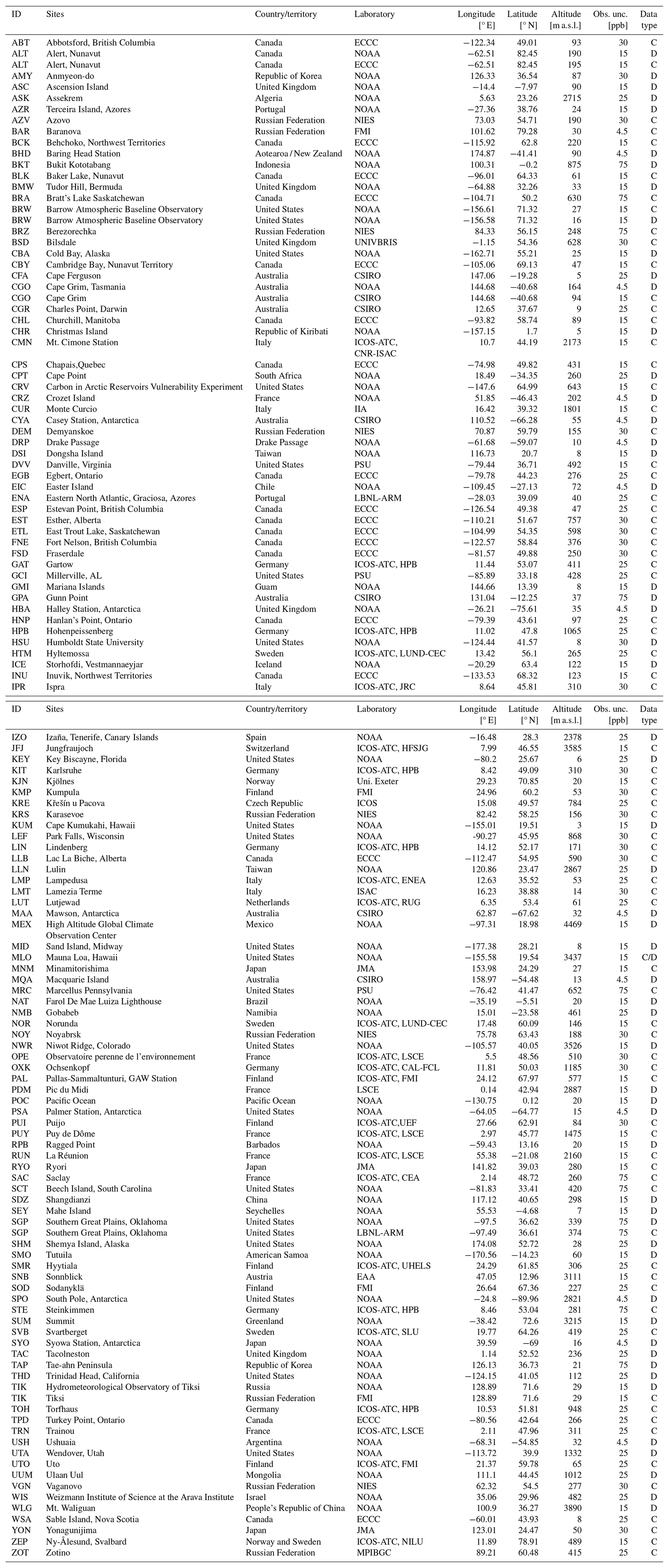
Table A2 List of the ICOS sites, data categories, PIs, and references for the sites used in InvSURF and evaluation.

Notholt et al. (2022)Morino et al. (2022c)Wennberg et al. (2022b)Deutscher et al. (2023b)Iraci et al. (2022)Wunch et al. (2002)Strong et al. (2022)Sussmann and Rettinger (2017)Liu et al. (2023)Blumenstock et al. (2017)Shiomi et al. (2022)Hase et al. (2022)Sherlock et al. (2022)Petri et al. (2023)Buschmann et al. (2022)Wennberg et al. (2022c)Warneke et al. (2022)Wennberg et al. (2022a)Te et al. (2022)De Mazière et al. (2022a)Morino et al. (2022a)Kivi et al. (2022)Morino et al. (2022b)Deutscher et al. (2023a)Zhou et al. (2022)

Table A3 The TCCON sites used for evaluation.

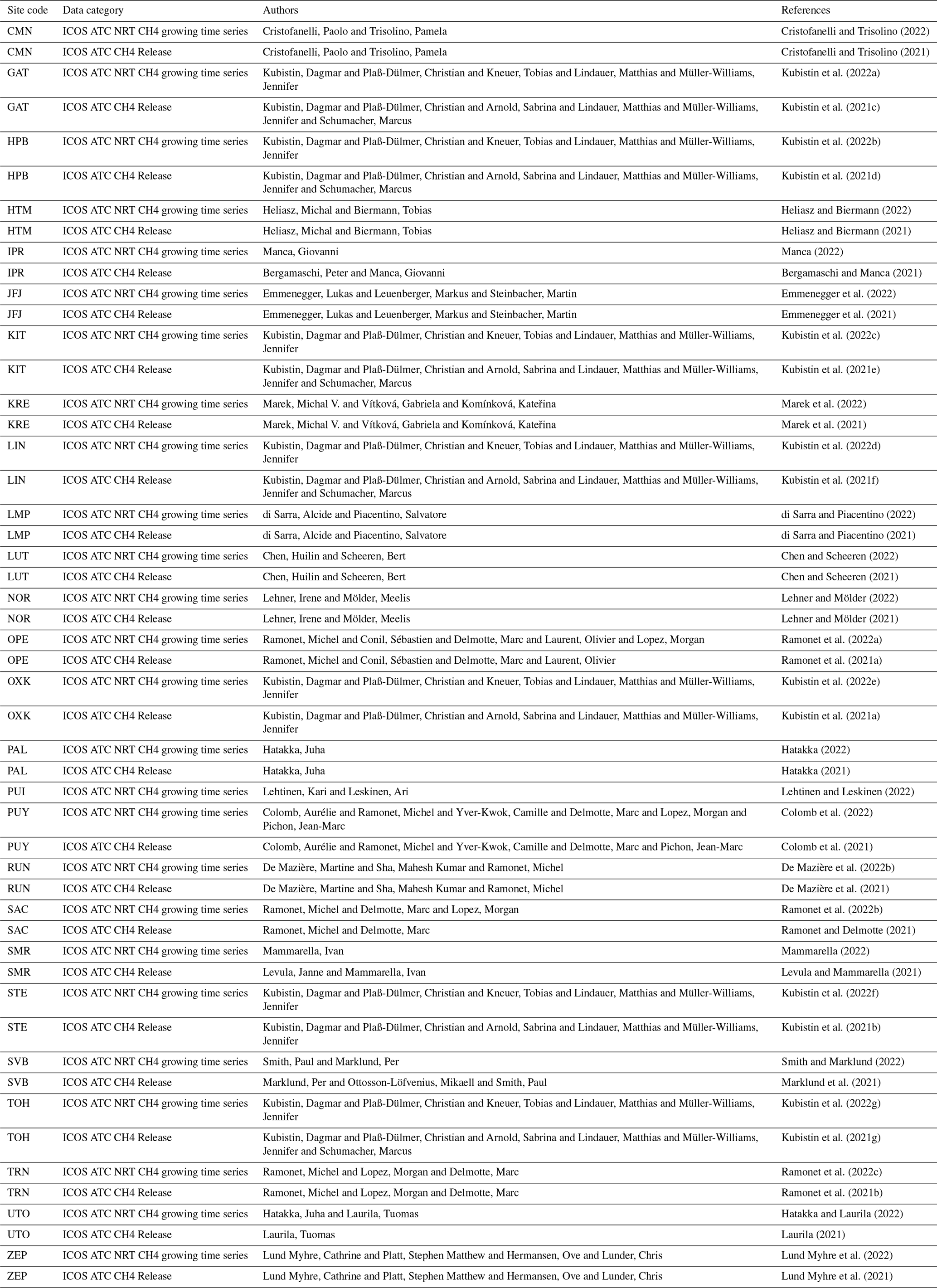
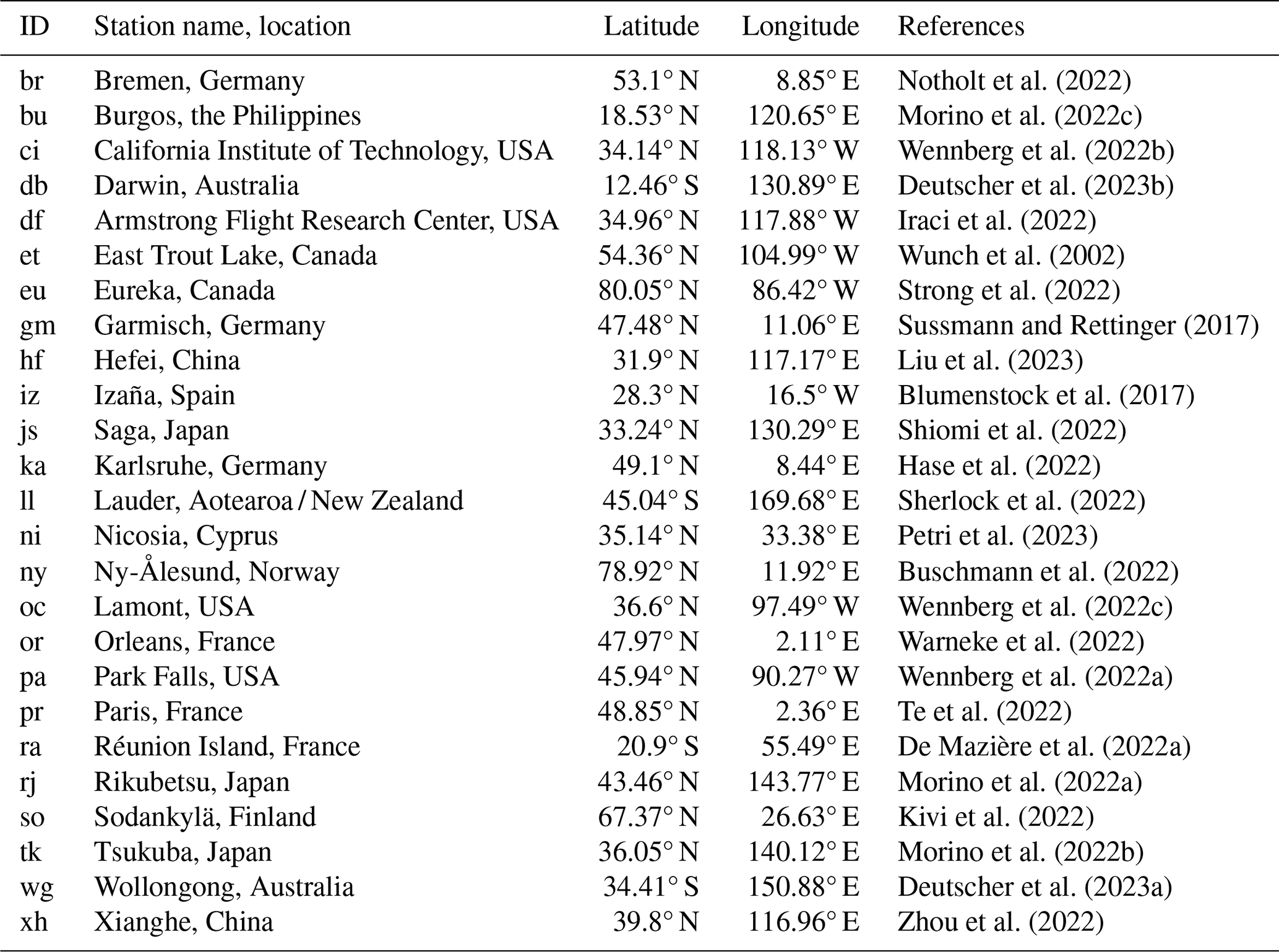
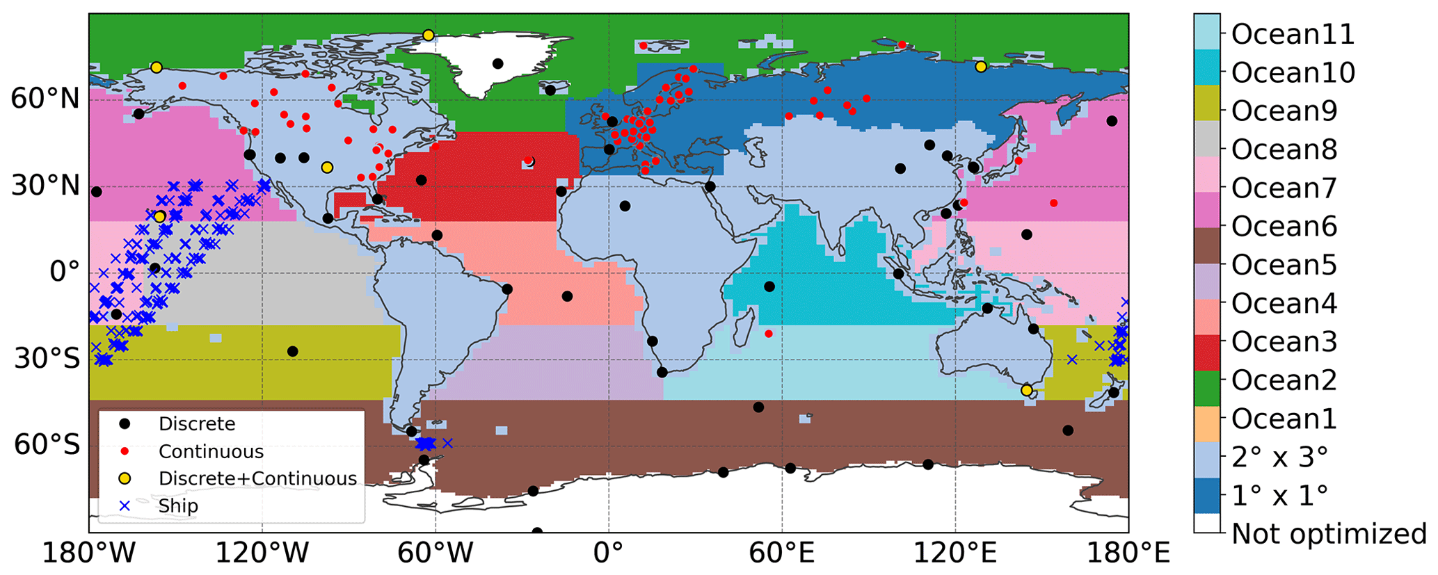
Figure A1 Location of ground-based surface observations (dots and x marks) assimilated in the InvSURF inversion experiment (see Sect. 2.4) and optimization regions used in CTE-CH₄ (background colours). Over land areas, the fluxes were optimized grid-wise and ocean-region-wise.

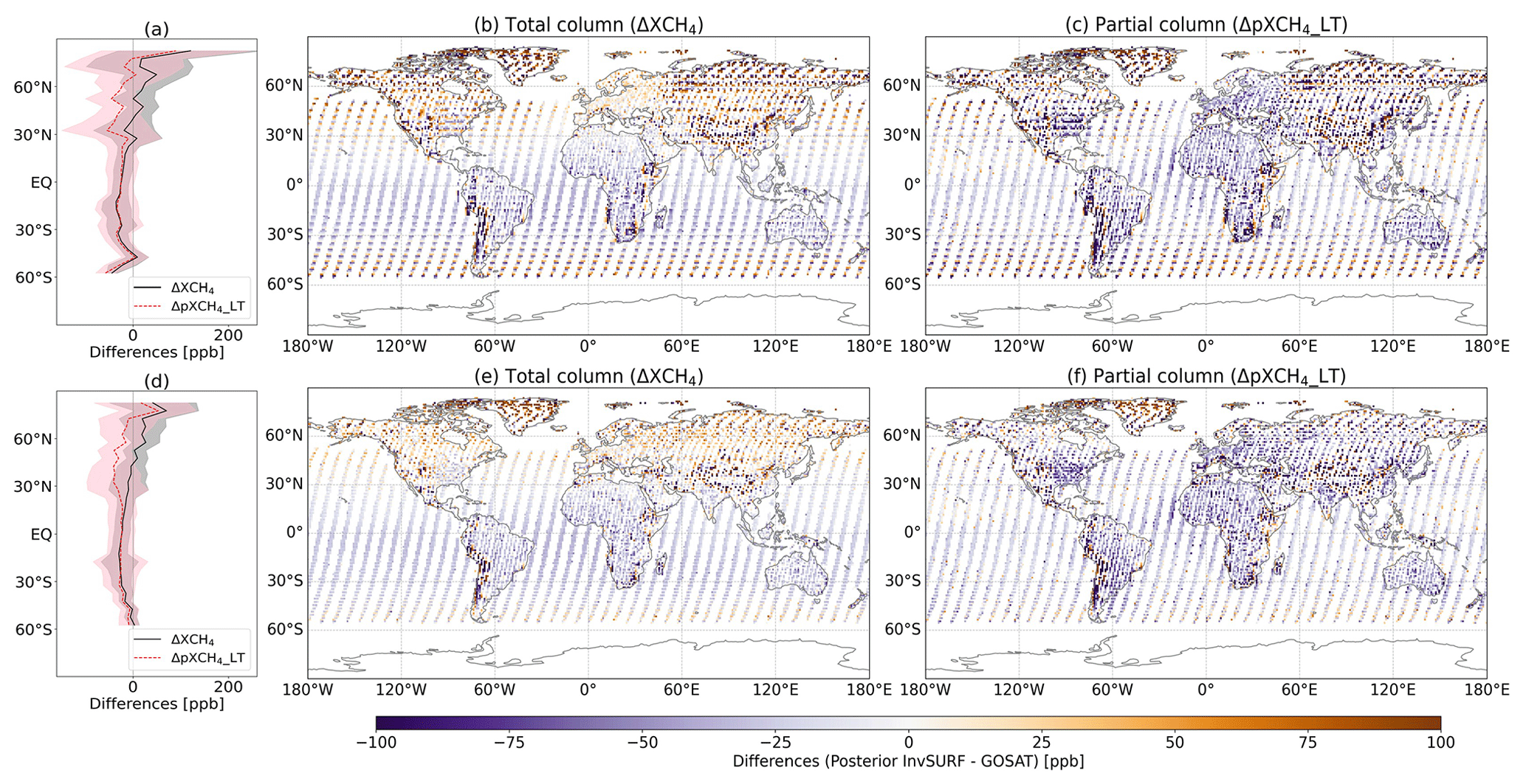
Figure A2 Mean differences between prior mole fractions and JAXA/GOSAT retrievals, averaged over 2016–2019. Panels (a) and (d) show 5° latitudinal means (solid line) with standard deviation (shaded area) and panels (b), (c), (e), and (f) 1°×1° grid means. Panels (a), (b), and (c) were calculated using TM5 with 1°×1° zoom over Europe and 6°×4° globally and (d–f) using 2°×3° (latitude × longitude) globally. Positive values indicate posterior InvSURF mole fractions being higher than the GOSAT retrievals.

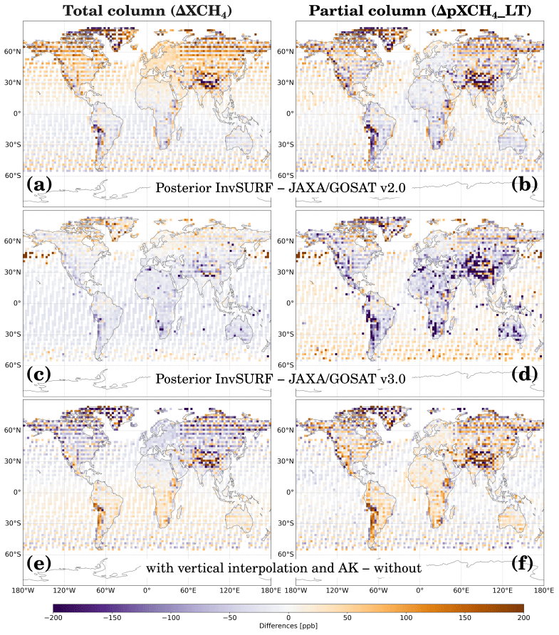
Figure A3 (a–d) Mean differences between posterior InvSURF and JAXA/GOSAT retrievals averaged over 2016 and at 2°×3° grids. Positive values indicate posterior InvSURF mole fractions being higher than the JAXA/GOSAT retrievals. Panels (a) and (b) compared to v2.0, without averaging kernels and vertical interpolation. Panels (c) and (d) compared to v3.0 with vertical interpolation and averaging kernels applied. Panels (e) and (f) are comparisons of modelled values between those calculated with vertical interpolation and AK (i.e. posterior InvSURF values from c and d) and those without interpolation and AK (i.e. posterior InvSURF values from a and b), illustrating the effect of interpolation and AK directly. Positive values indicate higher mole fraction values with interpolation and AK. Panels (a), (c), and (e) are comparisons of total columns, and panels (b), (d), and (f) are comparisons of lower-tropospheric partial columns.

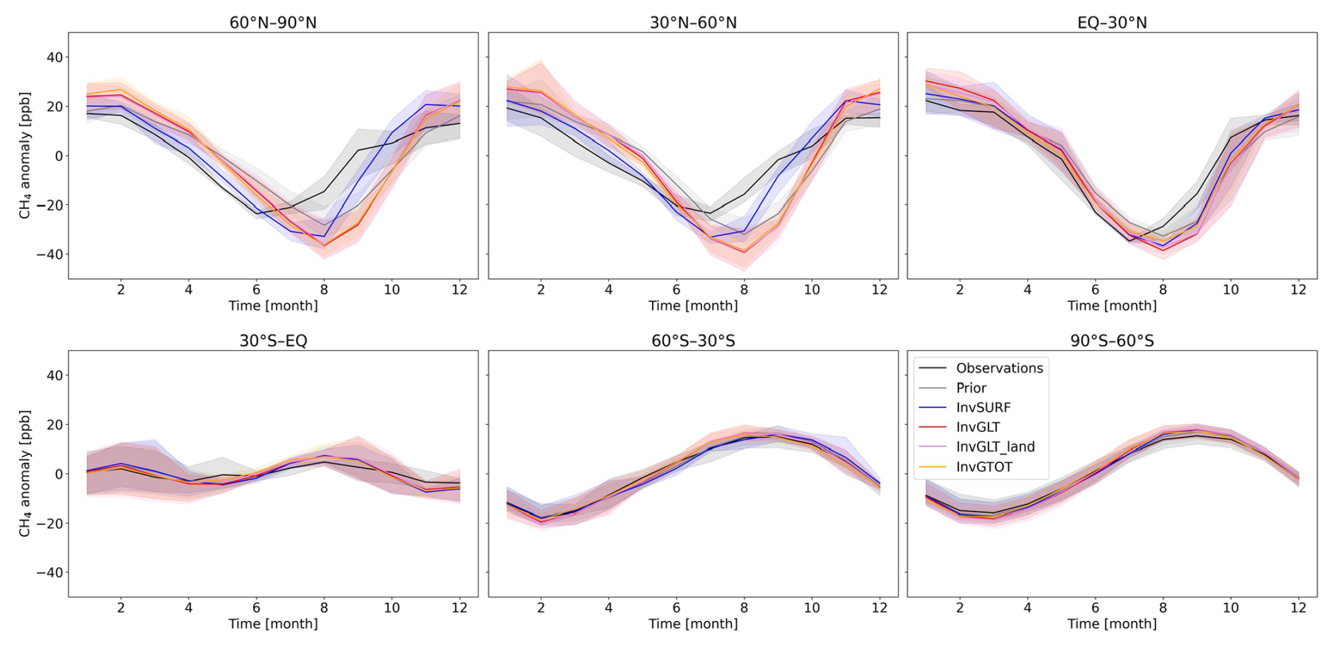
Figure A4 Detrended monthly average mole fractions at surface stations, assimilated in InvSURF. The data are averaged from 2016–2019 and at 30° latitudinal bands. Shaded areas are minimum and maximum of detrended monthly values within 2016–2019.

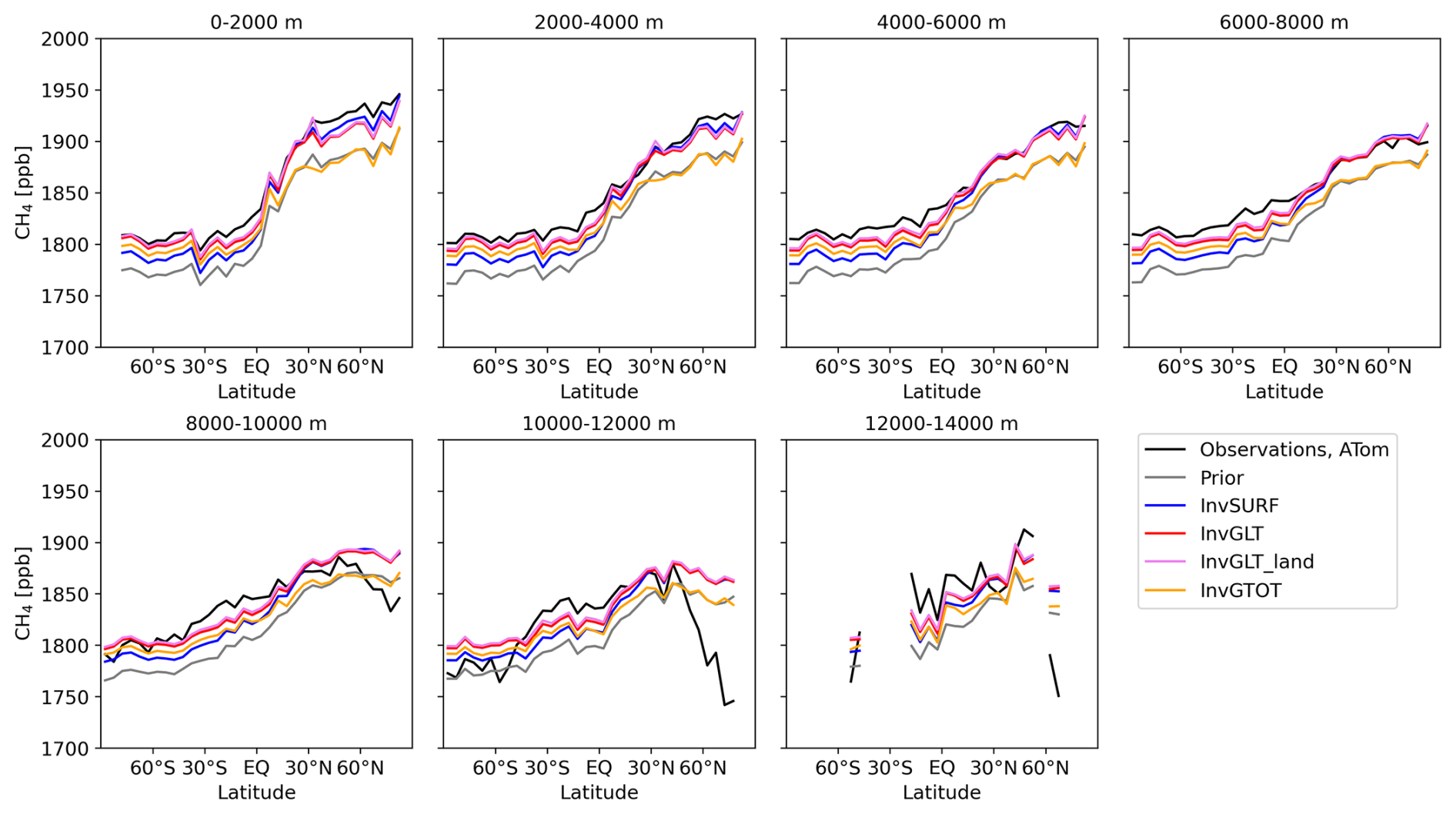
Figure A5 Mean atmospheric CH₄ at location and time of aircraft measurements from the Atmospheric Tomography Mission, averaged over 5° latitude bands and 2000 m altitude bands above sea level during 2016–2019.

Figure A6 As in Fig. A5, but means were subtracted at each altitude band.

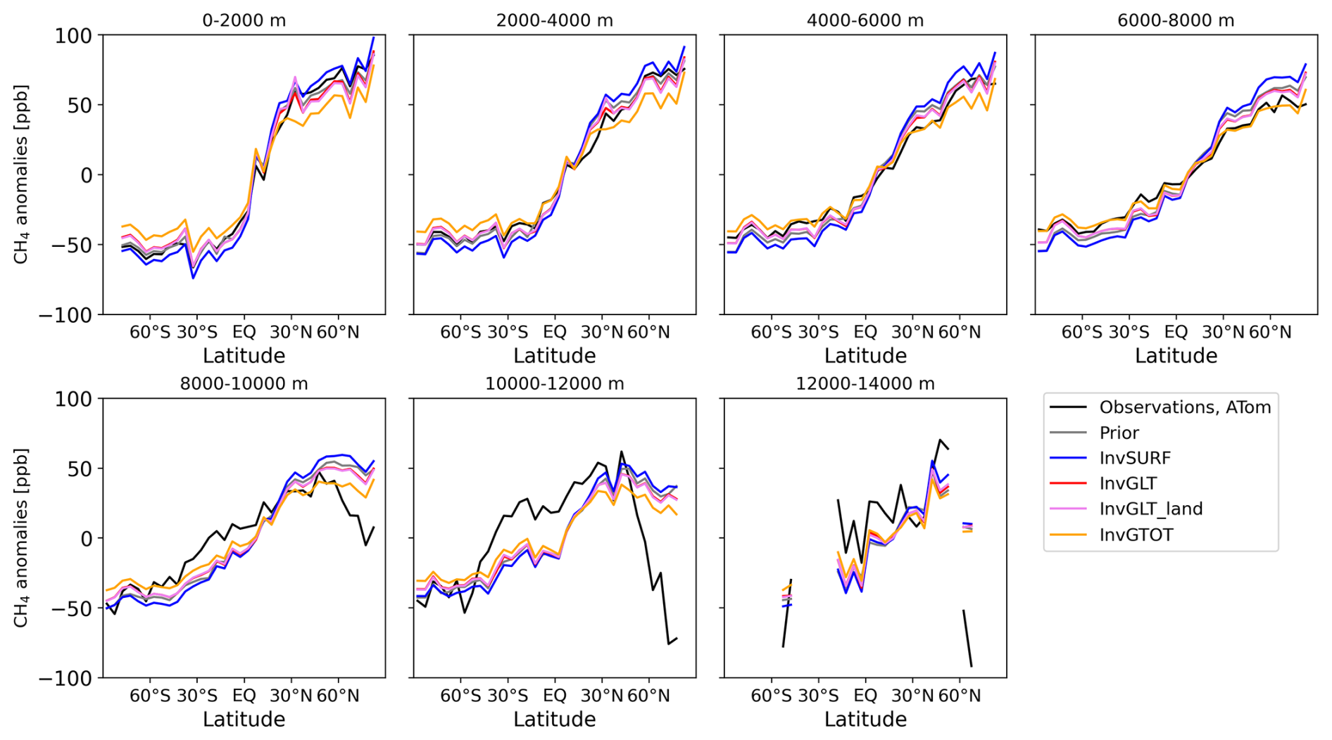
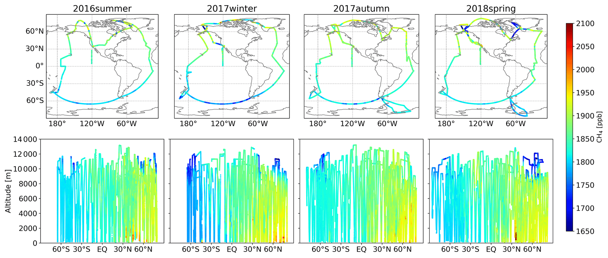
Figure A7 Observed CH₄ mole fractions from aircraft measurements of the Atmospheric Tomography Mission during the study period.

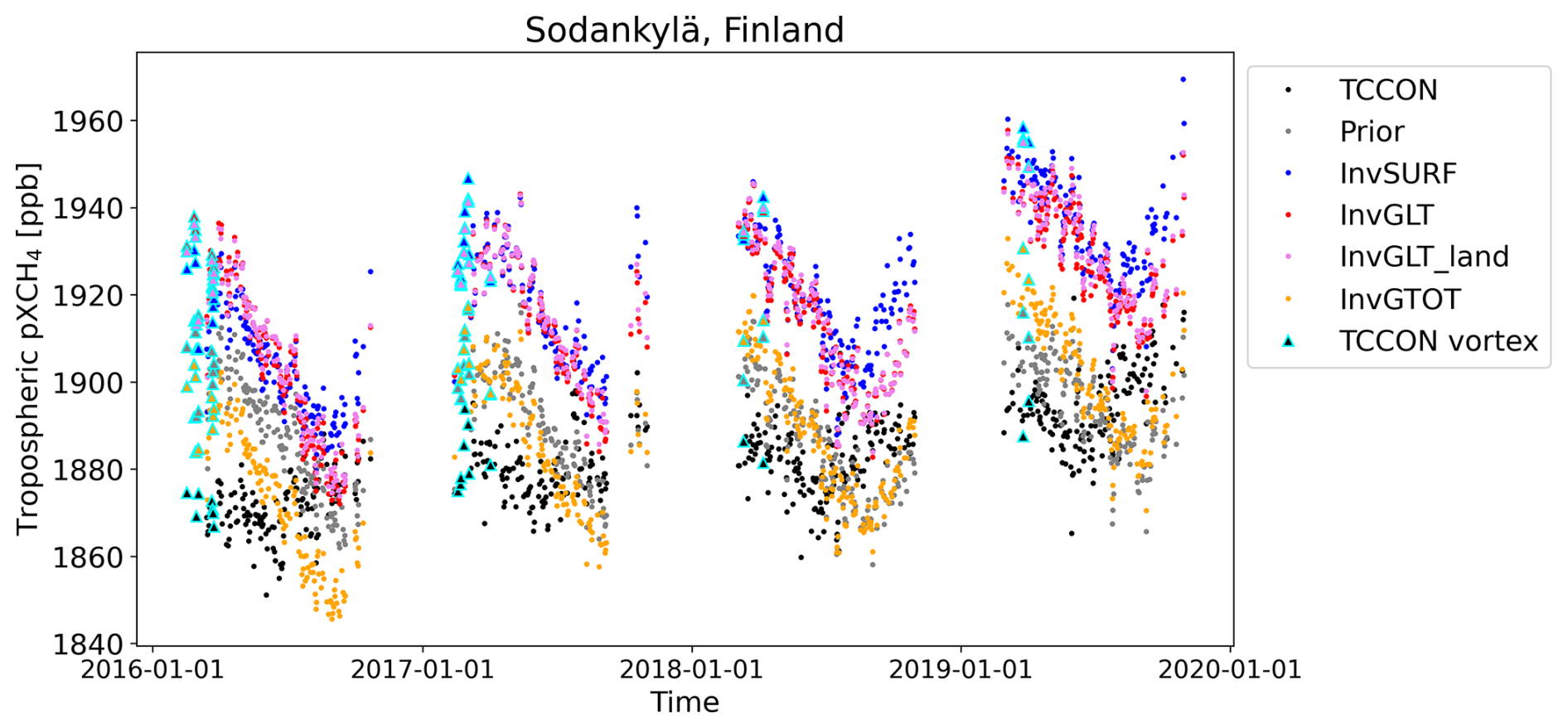
Figure A8 Daily averaged tropospheric partial columns at the Sodankylä TCCON station, Finland.

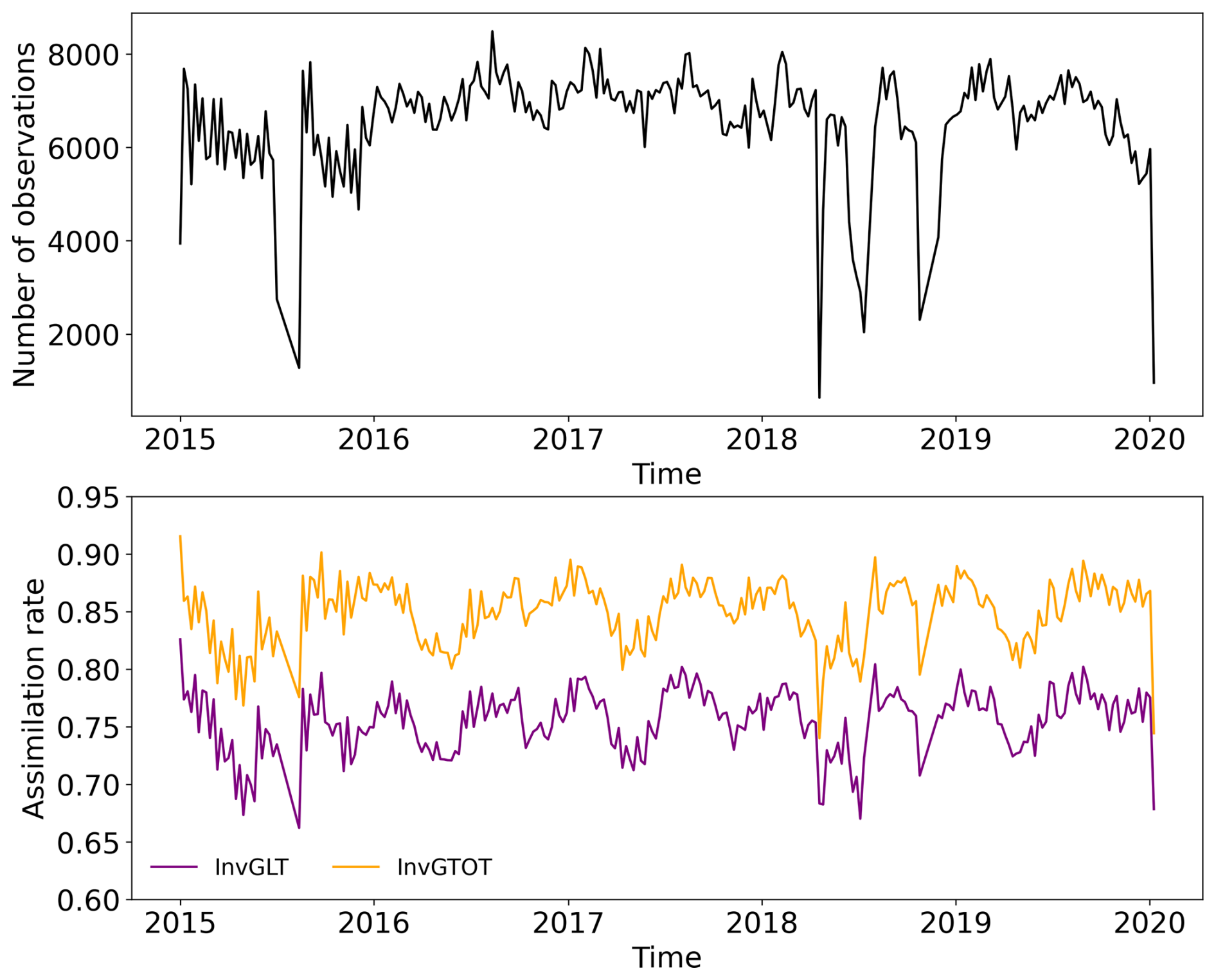
Figure A9 Global total number of JAXA/GOSAT observations per week and assimilation rates in GOSAT inversions. The x axis is weeks of optimization steps and not the actual time of observation.

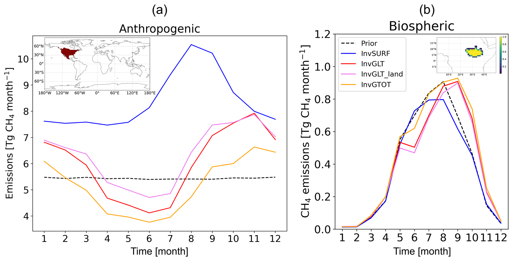
Figure A10 Average monthly CH₄ emissions in (a) southern North America and (b) South Sudan regions. The maps illustrate aggregated areas.