The skill at modeling an extremely high ozone episode varies substantially amongst ensemble simulation

Severe ozone pollution may occur in the Great Bay Area (GBA) when typhoons approach South China. However, numerical models often fail to capture the high ozone concentrations during the episodes, leading to uncertainties in understanding their formation mechanisms. This study conducted an ensemble simulation with 30 members (EMs) using the WRF-Chem model, coupled with a self-developed ozone source apportionment method, to analyze an extremely high ozone episode associated with Typhoon Nida in the summer of 2016. The newly proposed index effectively distinguished between well-performing (good) and poorly performing (bad) EMs. Compared to the bad EMs, the good EMs accurately reproduced surface ozone variations, particularly capturing the extremely high concentrations observed in the afternoon of 31 July. The formation of such high ozone levels was attributed to the retention of ozone in the residual layer at night and the enhanced photochemistry during the daytime. As Typhoon Nida approached, weak winds confined large amounts of ozone in the residual layer at night. The development of the planetary boundary layer (PBL) facilitated the downward transport of ozone aloft, contributing to the rapid increase in surface ozone in the following morning. The enhanced photochemistry was primarily driven by increased ozone precursors resulting from favorable accumulation conditions and enhanced biogenic emissions. During the period of high ozone concentrations, contributions from local and surrounding regions increased. Additionally, ozone from southeastern Asia could transport to the GBA at high altitudes and then contribute to surface ozone when the PBL developed.

1 Introduction

Tropospheric ozone, especially within the planetary boundary layer (PBL), has attracted much public attention because of its detrimental effects on human health and vegetation (Monks et al., 2015; Feng et al., 2019; Lu et al., 2020). As a typical secondary air pollutant, tropospheric ozone is primarily formed via photochemical reactions with the participation of nitrogen oxides (NO_x) and volatile organic compounds (VOCs) (Sillman, 1995; Xie et al., 2014; Li et al., 2019; Wang et al., 2019). Furthermore, the meteorological conditions play important roles in the chemical production and accumulation of ozone in the atmosphere, leading to severe air pollution (Ding et al., 2013a; Wang et al., 2017, 2022).

In the Great Bay Area (GBA; including the Pearl River Delta, Hong Kong SAR, and Macao SAR), China, ozone pollution is closely linked to the western Pacific subtropical high (WPSH) and northwest Pacific typhoon in summer and autumn (Gong and Liao, 2019; Shao et al., 2022; Liu et al., 2023). In particular, when a typhoon approaches this region, severe ozone pollution easily occurs (Deng et al., 2019; Qu et al., 2021). Many previous studies have suggested that when the GBA is at the periphery of a typhoon (Hu et al., 2010; Jiang et al., 2015), high solar irradiance and high temperature promote the ozone photochemical production (So and Wang, 2003; Ding et al., 2004), while unfavorable diffusion conditions increase the accumulation of ozone (Jiang et al., 2008; Li et al., 2022). Thus, high-ozone episodes may occur and persist in the period leading up to a typhoon landfall. Numerical simulations can help us quantitatively study the evolution of this type of ozone pollution (Li et al., 2022; Ouyang et al., 2022; Wang et al., 2022). Furthermore, numerical simulations can also help us separate the impacts of typhoons by comparing the base simulation with a sensitive simulation that removes the typhoon system (Hu et al., 2019). However, two key issues must be considered, as they may directly affect the accuracy and credibility of the simulation results. The first problem (Prob. 1) is related to whether the model can capture the variations in this type of ozone pollution, especially the extremely high ozone concentration. The second problem (Prob. 2) occurs because this type of ozone pollution is controlled by the competitive effects of the WPSH and typhoon; hence, erasing the typhoon system may increase the impact of the WPSH, which may lead to a high bias in the simulation results or even affect the final conclusions (Gilliam et al., 2015; Chatani and Sharma, 2018).

An ensemble simulation by perturbing meteorological factors in the initial and boundary conditions can offer a solution to the above problems. This method has a greater probability of capturing the spatial and temporal variations of air pollutants in extreme synoptic systems (Delle Monache et al., 2006; Zhang et al., 2007; Bei et al., 2014; Zhu et al., 2016), thereby providing more accurate data for relevant studies and yielding more reliable conclusions. More importantly, by comparing well-performing ensemble members (good EMs) with poorly performing EMs (bad EMs), we can better understand the impact of meteorology on ozone, which may help mitigate the uncertainties associated with Prob. 2.

In this study, we applied the Weather Research and Forecasting model (WRF; Skamarock et al., 2008) with Chemistry (WRF-Chem; Grell et al., 2005) coupled with an ozone source apportionment method (WRF-Chem-O3tag; Gao et al., 2016, 2017). By perturbing meteorological factors in the initial and boundary condition files, we constructed an ensemble simulation (including 30 EMs) to simulate the extremely high-ozone episode that occurred in the GBA associated with the approach of Typhoon Nida. By comparing the results of the EMs, we aimed to address the following issues: (1) more accurately capture the variation pattern and the extremely high concentration of surface ozone in the GBA, (2) elucidate the physical and chemical formation mechanisms of this ozone episode, and (3) quantify the changes in the ozone contributions from various geographical source regions during this pollution episode. The structure of this paper is as follows: Sect. 2 provides a description of the ozone episode, model system, and ensemble simulation. The results and discussion are presented in Sect. 3. The conclusions are summarized in Sect. 4.

2 The high-ozone episode and the methods applied in this study

2.1 The extremely high-ozone episode and the basic simulation

2.1.1 Severe ozone pollution when Typhoon Nida approached

Between 28 July and 3 August 2016, Super Typhoon Nida formed in the western Pacific and eventually made landfall along the coast of the GBA, resulting in severe disasters in South China, particularly in Guangdong Province and Guangxi Province. When Typhoon Nida approached the GBA, a high-ozone episode occurred in this region. During the afternoon of 31 July, the mean concentrations of surface ozone exceeded 200 µg m⁻³ (grade II of the national standard for the hourly ozone concentration) in most areas of the GBA (black square in Fig. 1b). Notably, the maximum concentration reached 366 µg m⁻³, recorded in Jiangmen at 14:00 local time (LT) on 31 July.

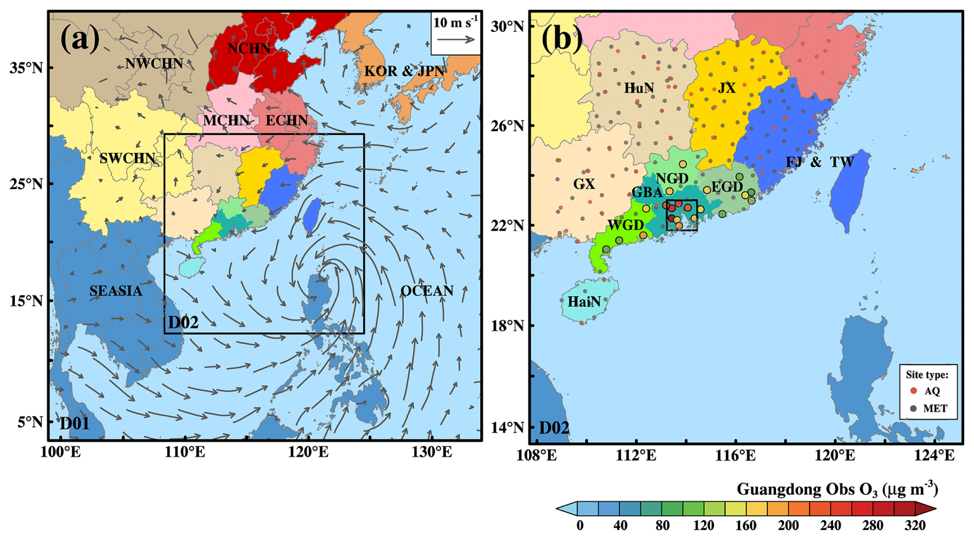
Figure 1 The model domains with the 10 m wind fields (a) and the measured ozone concentration in Guangdong Province (b) at 14:00 local time (LT) on 31 July 2016. The 10 m wind data originate from the European Centre for Medium-Range Weather Forecasts (ECMWF) Reanalysis V5 (ERA5) dataset. The locations of the meteorology and air quality observation stations are marked by grey and red dots in (b), respectively.

2.1.2 Basic simulation using the WRF-Chem model

In this study, we conducted a basic simulation using the WRF-Chem model. This model is a fully coupled 3D Eulerian model system that incorporates two-way online feedback between the meteorological model and the chemical transport model. It has been widely employed in air quality research and forecasting studies (Li et al., 2018; Gao et al., 2021; Yang et al., 2022; Huang et al., 2020, 2023). Regarding the model configuration, we established nested model domains (Fig. 1a). To simulate the lifetimes of both the ozone episode and Typhoon Nida, the parent domain (D01) covered most parts of East Asia and Southeast Asia. The simulation period spanned 00:00 on 25 July to 00:00 on 4 August 2016 (UTC). The first 2 d was designated as the spin-up period. The complete introduction of the model configuration and the datasets used can be found in the Supplement.

As shown in Fig. 2a, the comparison of the hourly ozone concentrations revealed that the basic simulation results (Bas) did not show good agreement with the observations (Obs) in the GBA. Although Bas could capture the diurnal variation well, it failed to simulate the ozone peaks during this episode. In particular, Bas significantly underestimated the maximum concentration that occurred in the afternoon of 31 July. Regarding the mean maximum daily 8 h average ozone (MDA8 O₃), the maximum value was reached on 31 July in Obs (Fig. 2b), whereas in Bas, the maximum value was reached on 30 July (Fig. 2c). The results suggested that Bas could not reproduce this ozone episode well, although the model settings have been widely employed and shown to be effective in many other air quality modeling studies. Hence, using the same model settings, we conducted an ensemble simulation in this study. We believe that this approach can enhance simulation accuracy and facilitate a better understanding of this high-ozone episode.

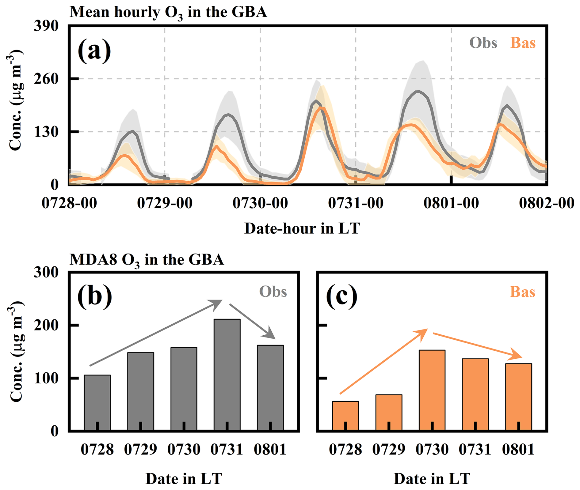
Figure 2 (a) The comparisons of mean hourly ozone in the GBA between the observations (Obs) and the basic simulation (Bas) and the mean maximum daily average ozone (MDA8 O₃) of Obs (b) and Bas (c) in the GBA.

2.2 Ensemble simulation and ozone source apportionment

For the ensemble simulation, all EMs were generated with the “cv3” background error covariance option in the WRF-3DVAR package via perturbation of the meteorological factors in the initial and boundary condition files. The horizontal wind components, potential temperature, and water vapor mixing ratio were perturbed with standard deviations of 2 m s⁻¹, 1 K, and 0.5 g kg⁻¹, respectively (Zhu et al., 2016; Xiao et al., 2023). This ensemble initialization method has been widely utilized in data assimilation and weather analysis (Meng and Zhang, 2008a, b; He et al., 2019; Chan et al., 2022). In this study, we used this method to create 30 EMs and run them separately. By comparing the simulated ozone concentrations with the observations, “good” and “bad” EMs could be distinguished on the basis of their performance. The formation of the ozone episode and its source contributions could then be quantitatively examined by contrasting the results of the good and bad EMs. In addition, the ensemble initialization method suggested that the purpose of this work is to study the impacts of meteorological fields on the formation of the high-ozone episode. Since we did not change anthropogenic emissions in the ensemble simulation, the impacts of anthropogenic emissions on ozone concentrations were not discussed.

2.3 Online ozone source apportionment method coupled with the WRF-Chem model

In this study, we also employed our ozone source apportionment method in the ensemble simulation to quantify the ozone contributions during this episode. Similar to the Ozone Source Apportionment Technology (OSAT; Yarwood et al., 1996), our method is a mass balance technique that aims to identify the ozone contributions from each geographical source region preset in the model domain. Due to its secondary pollutant properties, the photochemical production of ozone is attributed to the contributions of ozone precursors (NO_x and VOCs) emitted from the geographical source regions. In this method, the model domain is divided into several source regions, where ozone and its precursors are treated as independent variables. Because of the nonlinear relationship of ozone photochemistry, the ozone formation sensitivity (NO_x-limited or VOC-limited) will be determined for each grid at each time step. Then, the chemical production of ozone will be allocated based on the concentration ratio of the key ozone precursor (NO_x for NO_x-limited and VOCs for VOC-limited) from each source region. These variables will also undergo all the physical processes as the original variables experience during the simulation, but they will not interfere with the original simulation. In addition, the initial and boundary chemical conditions of the relevant species also need to be defined as sources to maintain the mass balance. More information on this method can be found in Gao et al. (2016, 2017).

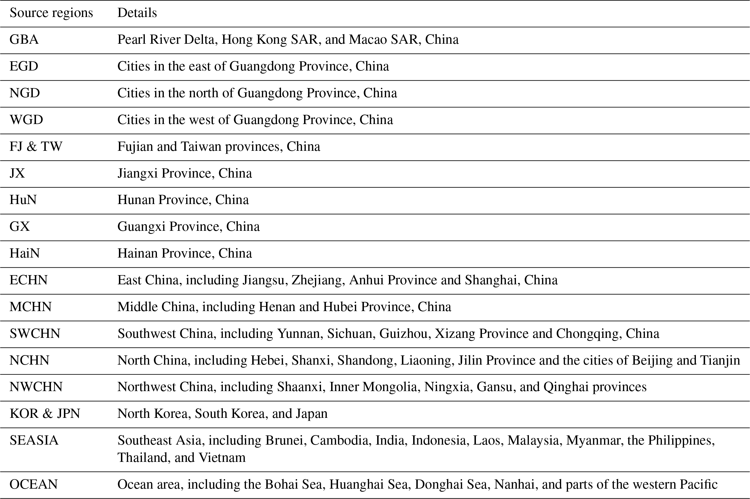
Before initiating the simulation, we need to establish geographical source regions for the ozone apportionment method. There were 17 geographical source regions in the model domain (Fig. 1a). The GBA, where we studied in this paper, was designated as one region. The other cities in Guangdong Province were categorized into three regions based on their relative locations to the GBA (Fig. 1b): east Guangdong (EGD), north Guangdong (NGD), and west Guangdong (WGD). For other areas in China, the region settings were defined according to administrative divisions. Source regions outside of China were defined based on national divisions. The marine areas in the model domain were established as one region. The detailed compositions of the various geographical source regions are listed in Table 1. In addition, the boundary conditions were defined as one region. which we referred to as O₃ inflow, as it can flow into the model domain and have a significant impact on ozone concentrations, which is typically treated as background ozone (Gao et al., 2017, 2020). The initial conditions of D01 and D02 were also defined as independent ozone contributions (INIT1 and INIT2, respectively).

Table 1 List of the geographical source regions in the model domain.

3 Results and discussion

3.1 EM selection and model validation

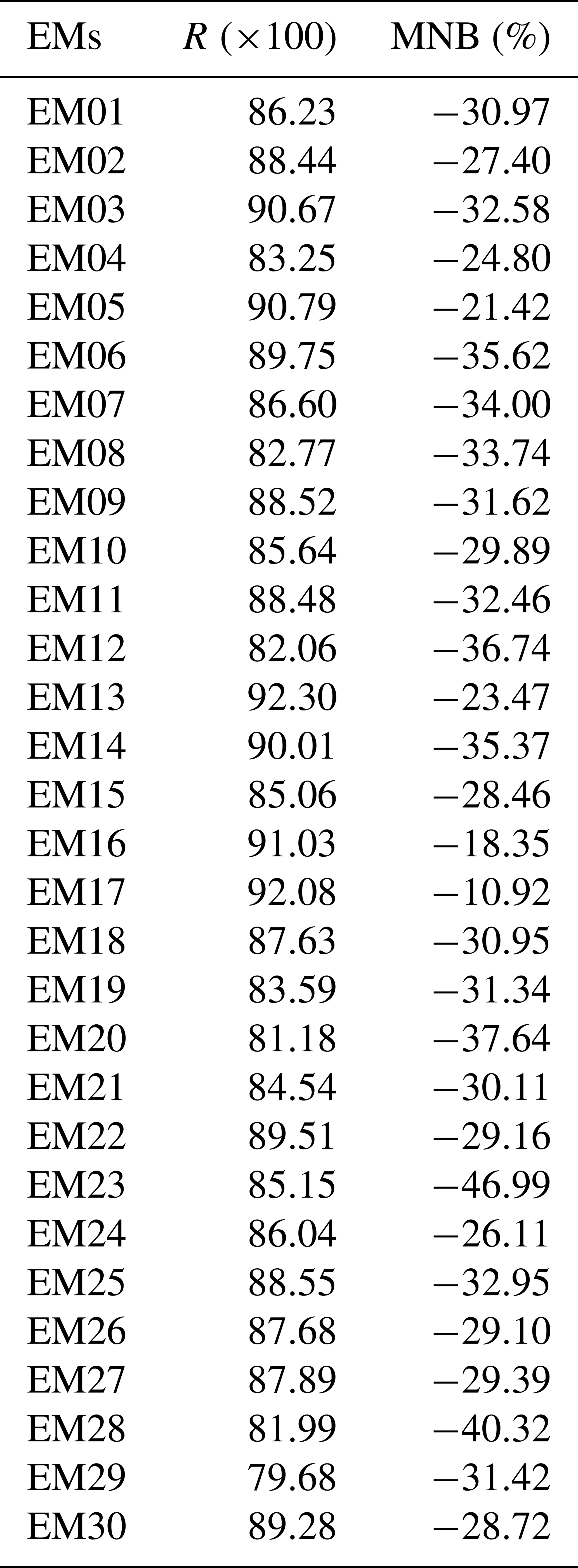
By comparing the observed ozone concentration with those simulated by each EM, we identified the EMs that could well reproduce the high-ozone episode in the GBA by considering the following two rules: (1) whether the EM could reproduce the variation pattern of the mean surface ozone in the GBA and (2) whether the EM could capture the maximum concentration that occurred in the afternoon of 31 July. Thus, two statistical metrics were determined to select good and bad EMs: the correlation coefficient (R) of the mean surface ozone in the GBA between the simulation and observation and the mean normalized bias (MNB) calculated from the simulated and observed ozone concentrations during the afternoon of 31 July (12:00–16:00 LT), when the maximum concentration occurred. The R and MNB of each EM are listed in Table 2. Among all the EMs, the values of R ranged from 0.79 to 0.92, indicating acceptable agreement with the variation pattern of observed ozone. The MNBs of all the EMs ranged from −46.99 % to −10.92 %. According to the U.S. EPA (2005, 2007), the recommended threshold values of MNB on ozone are ±15 %. Only EM17 could meet the criterion, while the other EMs did not.

Table 2 The R and MNB of surface ozone in the GBA between each EM and the observation.

It should be noted that both R and MNB were important to evaluate the model performance on ozone in this high-ozone episode; however, their validation results did not address a consistent conclusion. In order to draw a common conclusion, by considering the effects of both R and MNB, we introduced an index (I_dis) to quantitatively assess the performance of each EM. For each EM k, the index $I_{\mathrm{dis}}^k$ can be expressed as

$$\begin{array}{}\text{(1)}& \begin{array}{rl}{I}_{\mathrm{dis}}^k& =sqrt\left[(R^k\times \mathrm{100}-R_{\mathrm{best}}\times \mathrm{100}{)}^{\mathrm{2}}\right.\\ & \left.+{\left(\left|{\mathrm{MNB}}^k\right|-{\mathrm{MNB}}_{\mathrm{best}}\right)}^{\mathrm{2}}\right],\end{array}\end{array}$$

where R^k and MNB^k are the correlation coefficient and MNB between the observed ozone concentration and the simulated ozone concentration obtained from EM k, respectively. The values of R_best and MNB_best are 1 and 0, respectively. Thus, as shown in Fig. 3a, $I_{\mathrm{dis}}^k$, calculated using Eq. (1), represents the “distance” of the model performance of EM k from the best performance (red star). A smaller I_dis value indicates better performance of the EM. For clarity, $I_{\mathrm{dis}}^k$ is also represented by colors in Fig. 3a, where red indicates that the index is close to the “best”, while blue indicates that the index is far from the “best”.

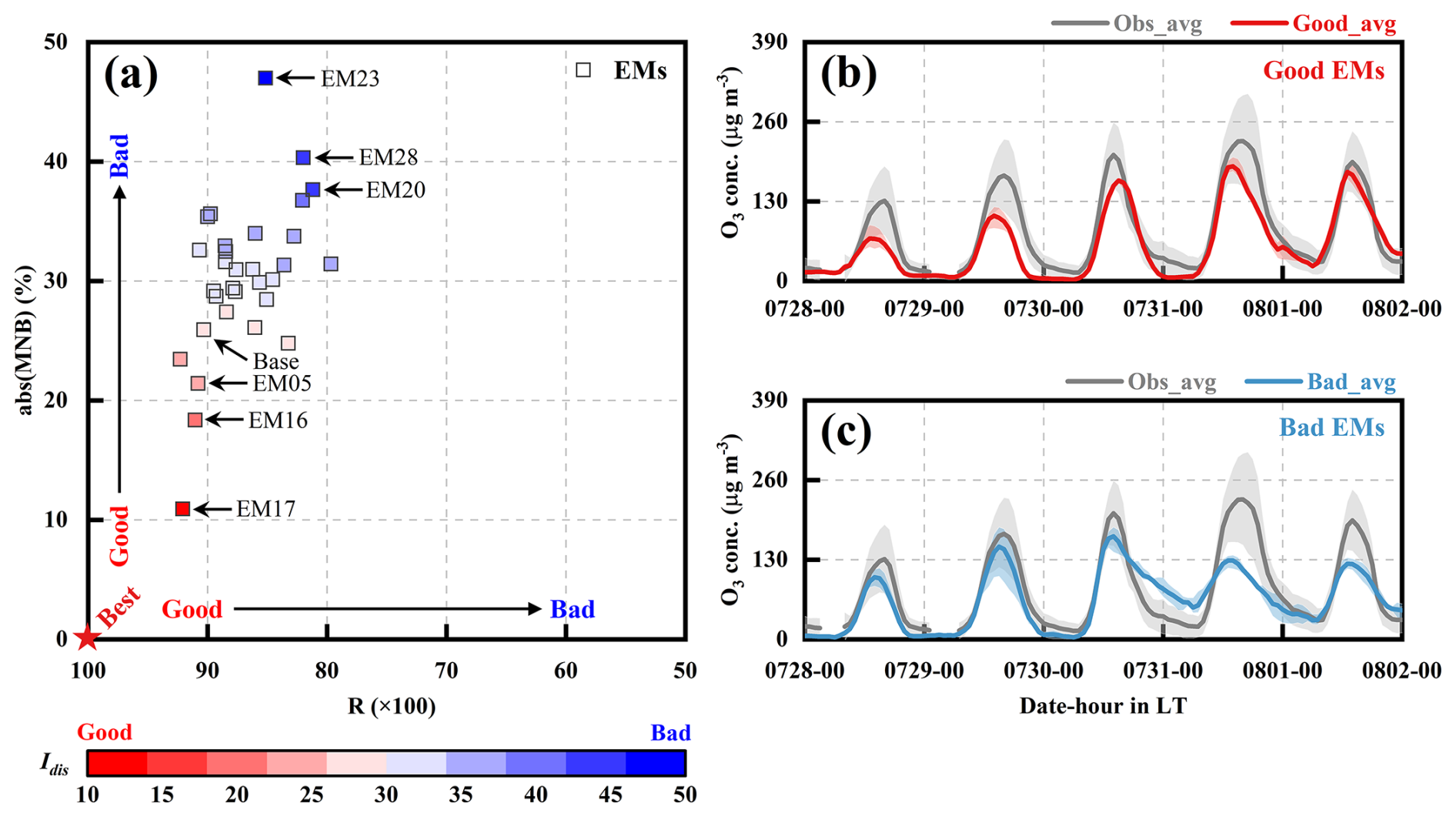
Figure 3 (a) Model performance of each EM on surface ozone in the GBA and comparisons between the observed and simulated surface ozone concentrations in the GBA for (b) good EMs and (c) bad EMs.

In Fig. 3a, I_dis (square) indicated that EM05, EM16, and EM17 were the top three members with performances closest to the best, suggesting that these three EMs more effectively reproduce the variations in ozone in the GBA. In contrast, the I_dis values of EM20, EM23, and EM28 were higher than those of the other EMs, indicating that they performed worse. Consequently, we classified EM05, EM16, and EM17 as good members, while EM20, EM23, and EM28 were classified as bad members. As shown in Fig. 3b, the comparison between the mean results of good EMs and the observations clearly revealed that the ozone time series of the good EMs agreed well with the observations and basically reproduced the variation pattern of ozone in the GBA during this episode, particularly the maximum concentration that occurred on 31 July. For the bad EMs (Fig. 3c), the time series of surface ozone exhibited an acceptable diurnal variation. However, they failed to capture the maximum ozone concentration on 31 July. In addition, for both the good and bad EMs, we also did the model validations on meteorological factors (temperature at 2 m, T2; wind speed, WS; and wind direction, WD) and NO₂ from hundreds of stations located in middle and southern China (Table S3). Statistical metrics revealed that, both inside and outside the GBA, the good EMs demonstrated better model performance than the bad EMs. For example, all the meteorological factors of the good EMs exhibited higher indices of agreement (IOAs) than those of the bad EMs did. Most variables of the good EMs exhibited lower biases than those of the bad EMs in all regions, except T2 outside the GBA and WD in all regions. The good EMs exhibited a satisfactory model performance and could effectively reproduce the high-ozone episode in the GBA.

3.2 Physical and chemical causes of the extremely high ozone concentration on 31 July

3.2.1 Process analysis of the average time series of surface ozone in the GBA

For surface ozone in the GBA, the average time series of the good and bad EMs (abbreviated as ozone_good and ozone_bad, respectively) are shown in Fig. 4a. The time series exhibited similar diurnal variations and concentrations from 28 July to the afternoon of 30 July. The two ozone time series then began to vary differently, and the differences increased until the afternoon of 31 July. Specifically, compared with that of ozone_bad, the time series of ozone_good declined more sharply in the afternoon of 30 July, and the concentration remained relatively low until the early morning of 31 July (Stage I; light-orange shaded area). From 08:00 LT on 31 July, the time series of both ozone_good and ozone_bad began to increase, and the trends persisted until the afternoon, when high ozone concentrations occurred (Stage II; dark-orange shaded area). Notably, ozone_good increased much more than that of ozone_bad did, resulting in the maximum concentration during this high-ozone episode in the GBA. The variation pattern was also consistent with that in the observations. As mentioned above, the relatively high maximum concentration of ozone_good may be attributed to the significant differences between ozone_good and ozone_bad from the afternoon of 30 July to the afternoon of 31 July.

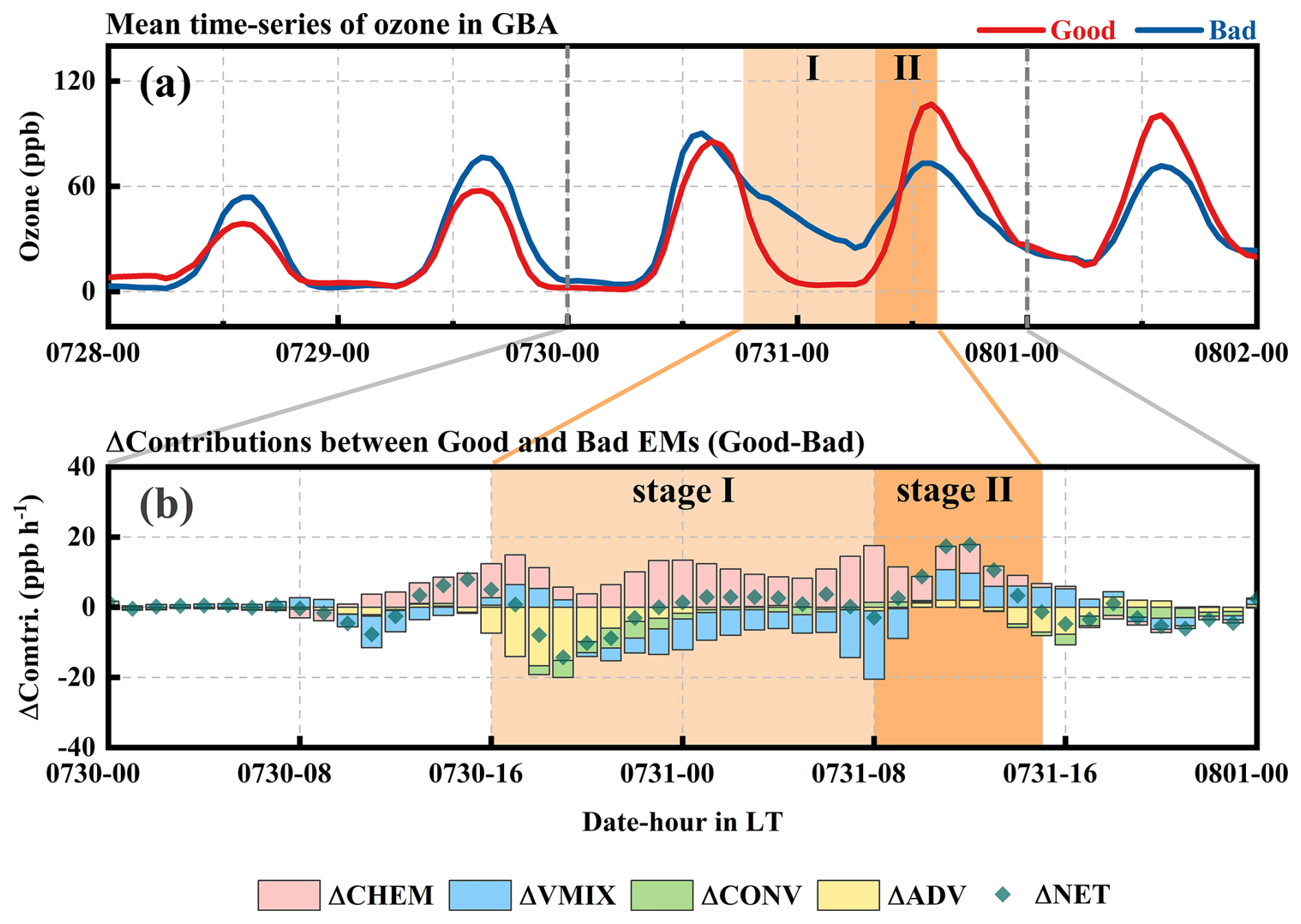
Figure 4 (a) Averaged time series of ozone_good and ozone_bad in the GBA and (b) the differences in each ozone contribution between the good and bad EMs (good − bad) from 30 to 31 July. CHEM = chemistry, VMIX = vertical mixing, CONV = convection, ADV = advection, NET = net contribution.

The changes in ozone contributions between good and bad EMs (good − bad) could help us clarify the chemical and physical causes of the extremely high ozone concentration on 31 July (Fig. 4b). ΔNET is calculated as the sum of all differences from each process between the good and bad EMs, which can represent the relative changes in ozone_good relative to ozone_bad. For example, when both ozone_good and ozone_bad increased at Stage II, the positive ΔNET value indicated a more significant increase in ozone_good. At these two stages, ΔCHEM, ΔADV, and ΔVMIX significantly contributed to ΔNET. At Stage I, although both ozone_good and ozone_bad decreased, the negative values of ΔNET during 18:00–21:00 on 30 July suggested that ozone_good decreased more significantly, which was attributed primarily to ΔADV. At Stage II, ozone_good increased more than ozone_bad did since ΔNET became positive. The budget of ΔNET suggested that the significant increase in ozone_good resulted from the combined effects of ΔCHEM and ΔVMIX. Hence, it could be concluded that the extremely high concentration of ozone_good that occurred in the afternoon of 31 July could be directly attributed to the ozone contributions from chemical and vertical mixing processes. In addition, ΔADV during the evening of the previous day also contributed to the extremely high concentration. In the following section, we will discuss the causes of the extremely high ozone concentration from physical and chemical perspectives.

3.2.2 Physical cause of the extremely high ozone concentration

Among the physical processes, VMIX was the direct contributor to the high concentration of ozone_good from 10:00 to 15:00 LT on 31 July. Here we took the situation at 11:00 as an example (Fig. 5). By comparing the VMIX of ozone_good with that of ozone_bad (ΔVMIX in Fig. 5a), the negative values aloft and positive values near the surface suggested that more ozone from ozone_good was entrained downward to the surface, leading to a greater increase in ozone at ground level. As the two key factors of VMIX (Gao et al., 2018), the differences in the vertical exchange coefficient and the vertical ozone profile between the good and bad EMs could explain the significant contribution of VMIX in good EMs. In the morning of 31 July, there were no obvious differences between the good and bad EMs (Fig. 5b). However, the vertical ozone profiles (Fig. 5c) revealed that ozone_good exhibited higher vertical gradients from the surface to the top of the PBL. Under these conditions, compared with the bad EMs, the good EMs showed more transport of ozone from the top of PBL to surface, despite similar vertical exchange intensities.

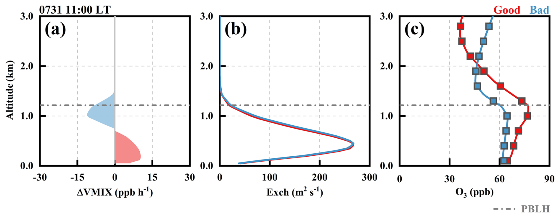
Figure 5 The vertical profiles of the changes in VMIX between good and bad EMs (good − bad) (a), exchange coefficients (b) and ozone concentrations of good and bad EMs (c) at 11:00 LT on 31 July.

The greater vertical gradients of ozone from good EMs occurred not only in the morning of 31 July but also in the previous evening. As shown in Fig. 6a, the vertical distribution of the difference in ozone between good and bad EMs (ΔOzone) showed positive values aloft and negative values in the lower layers from the evening of 30 July to the morning of 31 July. This indicated that good EMs exhibited greater vertical gradients of ozone during this period. Notably, the positive ΔOzone values aloft were even greater during the morning of 31 July, which could further increase the vertical gradient of ozone. ΔNET (Fig. 6b) revealed a negative zone (blue square) at altitudes of 0–750 m from 18:00 to 23:00 LT on 30 July and a positive zone (red square) at altitudes of 1000–1500 m from 05:00 to 11:00 LT on 31 July. These two changes were the direct causes of the vertical structure. By separating ΔNET into changes in physical and chemical contributions (Fig. 6c–f), it could be observed that ΔADV exhibited the same features (the negative and positive zones in Fig. 6b) as ΔNET did at the same altitude during the same period, suggesting that the significant vertical gradients of ozone_good were primarily caused by distinct ΔADV values at different levels during various periods.

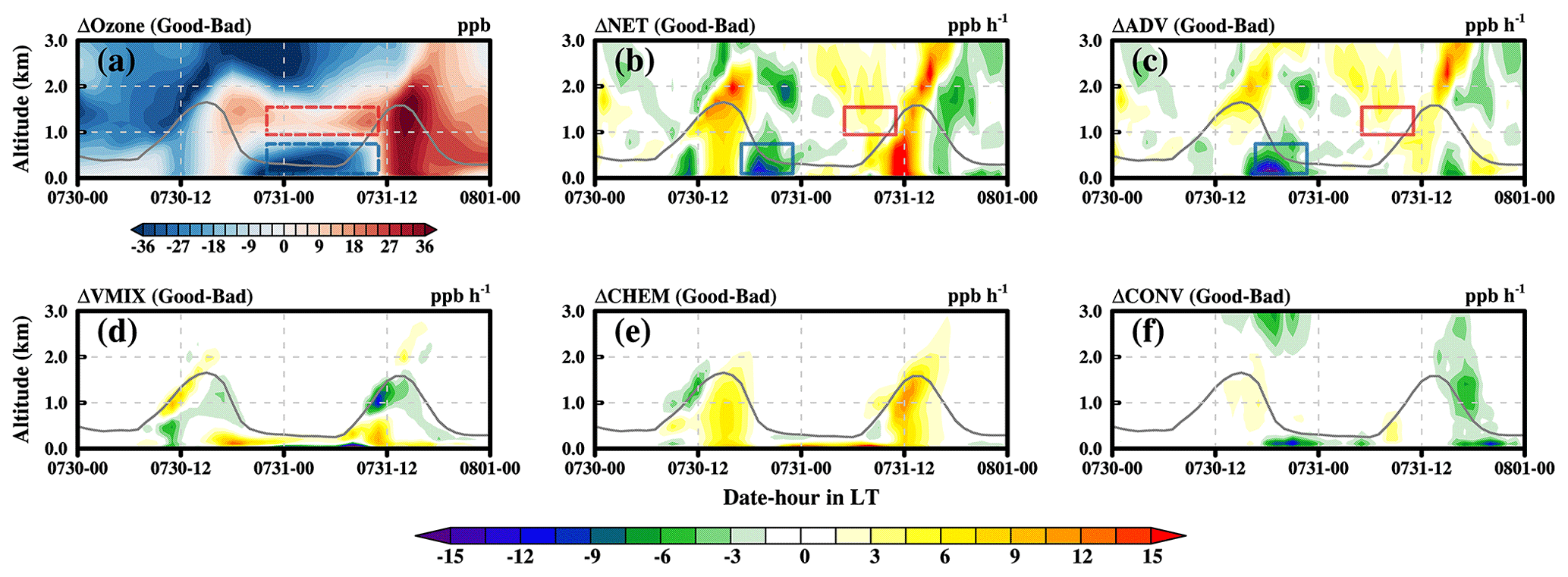
Figure 6 The vertical distributions of the changes in ozone (a) and its contributions (b–f) between good and bad EMs (good − bad).

The contribution of ADV is influenced by wind fields and ozone spatial distributions (Gao et al., 2017). The mean distributions of the ozone concentration and wind fields are shown in Fig. 7. During the evening of 30 July, the good EMs indicated southwest winds in the GBA in the lower layers (Fig. 7a). With the transport of southwesterly winds, the low concentrations of ozone over sea areas (upwind regions) could be transported to the GBA, leading to a decrease in ozone. However, the bad EMs showed that the GBA was controlled by easterly winds (Fig. 7b). The ozone in the upwind region was approximately equal to or even higher than that in the GBA, which did not cause a significant decrease in ozone levels. Thus, the concentrations of ozone_good were lower than those of ozone_bad in the lower layers of the GBA in the evening of 30 July (Fig. 7d). The significant vertical ozone gradient was more closely associated with the increase in ozone aloft in the morning of 31 July (Fig. 7e–h). In the higher layers, the good EMs exhibited high ozone concentrations and approximate static winds across the GBA, which was favorable for ozone retention (Fig. 7e). However, the bad EMs exhibited stronger east winds but lower ozone concentrations in upwind regions, which might have led to a decrease in ozone over the GBA (Fig. 7f). Thus, the concentrations of ozone_good were higher than those of ozone_bad over the GBA during the morning of 31 July (Fig. 7h). In addition, the good EMs showed weaker winds than the bad EMs did at the two stages (Fig. 7c and g, respectively). Especially in the higher layers, the weak winds played an important role in the increased ΔOzone value.

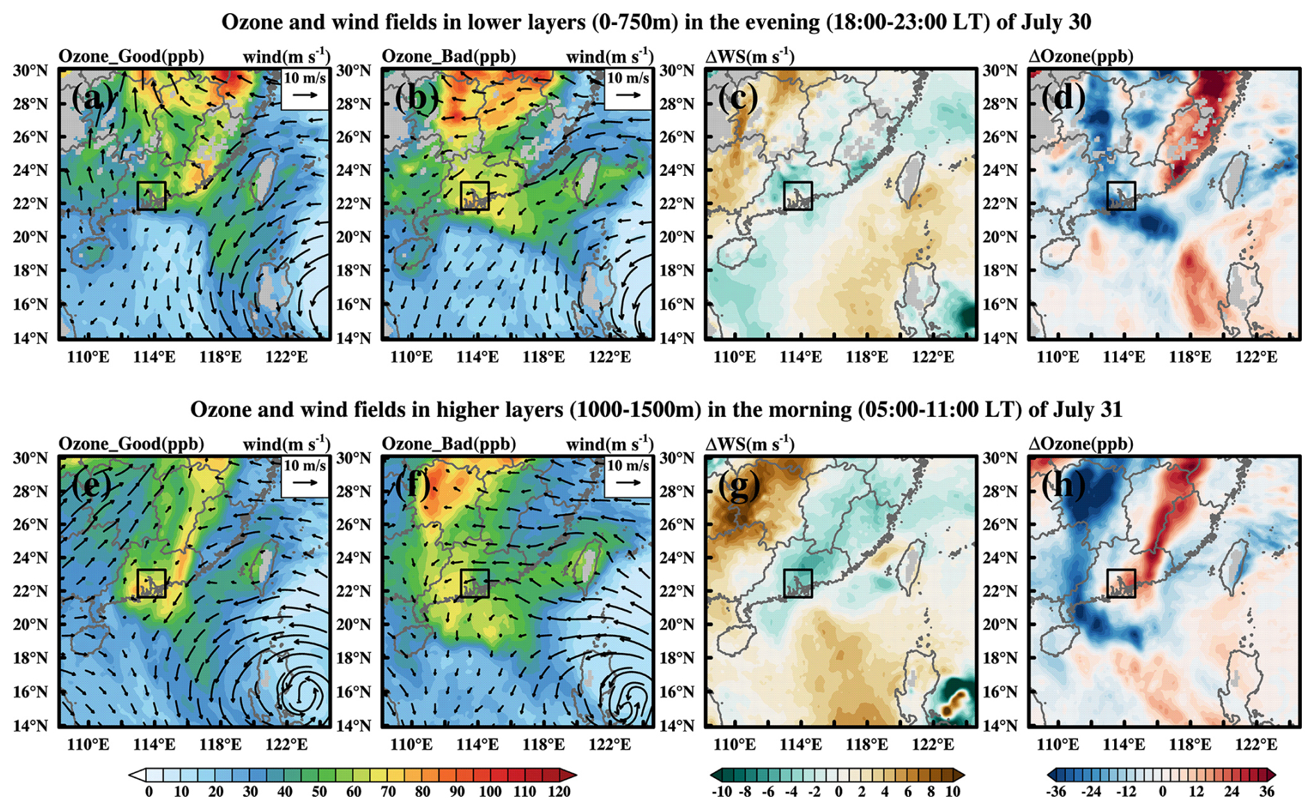
Figure 7 Mean distributions of the ozone concentration and wind fields and their respective differences between the good and bad EMs (good − bad) in the lower (a–d) and higher layers (e–h).

The changes in WS between good and bad EMs (good − bad; Fig. 8a) showed that the WS of good EMs was weaker than that of bad EMs from the surface up to nearly 1700 m. The weak wind could confine ozone in the residual layer from the evening of 30 July to the early morning of 31 July. To evaluate the model performance in WS, we collected the vertical sounding observations of wind speed from four stations in the GBA (the station codes and locations are listed in Table S2). By comparing the observations with the simulations, it can be concluded that the WS of good EMs agreed better with the observations, as their differences were relatively small in the lowest range of 2 km (Fig. 8b). In contrast, the bad EMs performed worse. Most of the time, the WS of the bad EMs was greater than that of the observations, especially during the evening of 30 July and the morning of 31 July (Fig. 8c). By comparing the differences (Fig. 8b and c), especially in areas (solid squares) where ADV significantly differed (mentioned in Fig. 6c), the WS of the good EMs was closer to the observations, which not only indicates the better model performance of the good EMs for the vertical features of WS but also indicates the important contribution of static winds to the formation of high ozone levels in the residual layer.

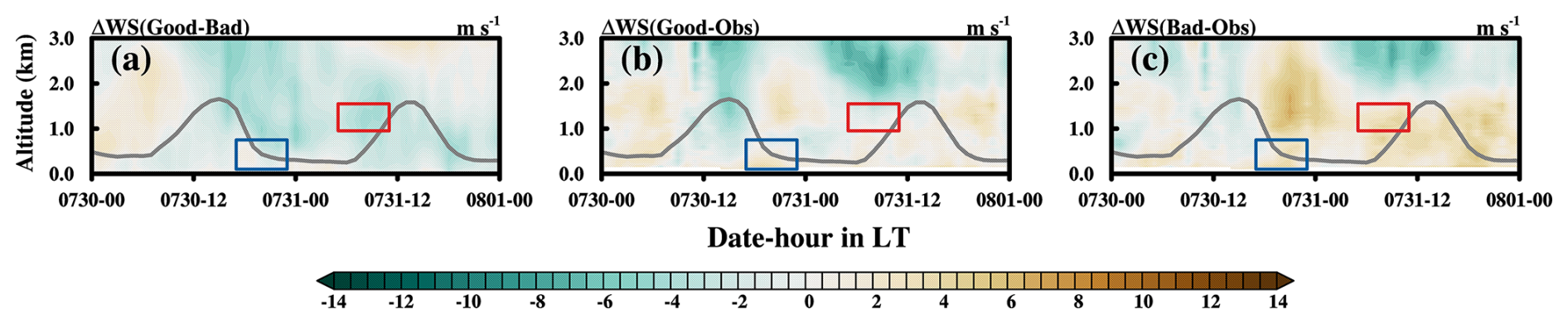
Figure 8 Vertical distributions of three differences of WS: (a) good − bad, (b) good − obs, and (c) bad − obs.

3.2.3 Chemical cause of the extremely high ozone concentration

Enhanced ozone contribution of chemistry (CHEM_Ozone) was another key contributor to the extremely high ozone concentration. The changes in CHEM_Ozone (ΔCHEM_Ozone) were positive within the PBL from 11:00 to 16:00 LT (Fig. 9a), suggesting that the photochemistry in the good EMs was significantly greater than that in the bad EMs. Notably, enhanced photochemistry was more significant in the middle and upper layers of the PBL. Correspondingly, the changes in the NO_x contribution of chemistry (ΔCHEM_NO_x) showed negative values, which also indicated that enhanced ozone photochemistry occurred in the good EMs.

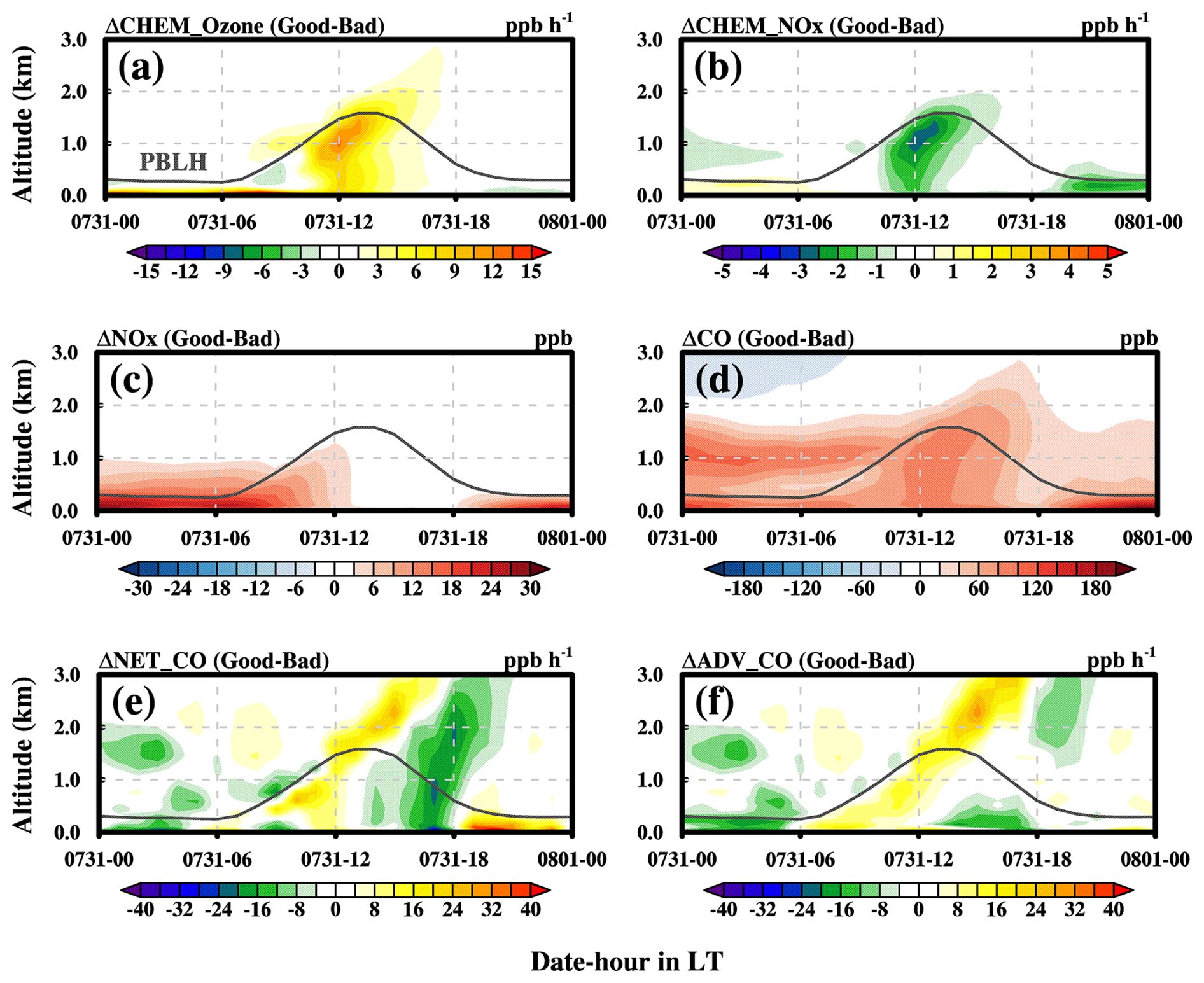
Figure 9 Vertical distributions of the changes in CHEM of ozone and the inducing causes on 31 July. (a) Changes in CHEM of ozone, (b) changes in CHEM of NO_x, (c) changes in the concentrations of NO_x, (d) changes in the concentrations of CO, (e) changes in NET of CO, and (f) changes in ADV of CO.

The photochemical production of ozone primarily depends on ozone precursors and chemical reaction constants (Monks et al., 2015). Although the meteorological factors differed significantly between the good and bad EMs, the relevant photochemical reaction constants, such as the photolysis rates (Fig. S2), did not show significant differences in the PBL during the daytime. Thus, the enhanced photochemical production of ozone in the good EMs could be attributed primarily to the increase in ozone precursors. Taking NO_x as an example, the changes in NO_x (ΔNO_x) showed positive values in the morning, which suggested that the good EMs contained more ozone precursors within the PBL and could enhance ozone photochemistry. Interestingly, ΔNO_x could approach 0 ppb in the afternoon, which did not align with the significant increase in ΔCHEM_Ozone during this period. This discrepancy arises because photochemical reactions are rapid, leading to the swift consumption of ozone precursors during their accumulation. Thus, although the meteorological conditions favored the accumulation of ozone precursors, they were consumed quickly by photochemical reactions.

To better characterize the accumulation of ozone precursors, we applied CO as a substitution. Since CO changes induced by chemistry are much lower than those induced by physical processes, the distributions of CO better reflect the accumulation of gaseous pollutants (Ding et al., 2013b). As shown in Fig. 9d, the changes in CO showed positive values during the whole day, which indicated the concentrations of CO in the good EMs were much higher than those in the bad EMs within the PBL not only in the morning but also in the afternoon. By comparing the changes in NET of CO (Fig. 9e) with those in ADV of CO (Fig. 9f), it could be concluded that the increased CO was primarily attributed to the advection process within the PBL during the daytime. The enhanced CO contribution of ADV was also due to weak winds. As shown in Fig. 8a, the WS in the good EMs was lower than that in the bad EMs within the lowest 2 km during the daytime. Lower WS favored the accumulation of gaseous pollutants, particularly ozone precursors, which could subsequently enhance the ozone photochemistry.

In addition, high temperature is a key factor in enhancing biogenic emissions, which can increase the concentrations of VOCs in the atmosphere. Comparative analysis showed that the temperatures in the good EMs were higher in most parts of Guangdong Province (GD) and Jiangxi Province (JX) (Fig. 10a). Consequently, increased temperature could lead to the enlargement of leaf stomata, thereby emitting more biogenic VOCs (BVOCs) into the atmosphere (Guenther et al., 2006, 2012). Adopting isoprene as an example (Fig. 10b), the changes in the isoprene induced by biogenic emissions (ΔBE_ISOP) closely matched the changes in T2 (ΔT2), indicating that the higher temperature in the good EMs resulted in increased biogenic VOCs in the atmosphere, especially in the western and northern parts of GD. Northwest winds facilitated the transport of more VOCs to the GBA, promoting the photochemical production of ozone, which is another important chemical cause of the extremely high ozone concentration on 31 July. Our results support the findings of a previous study that highlighted the impact of BVOCs on ozone pollution in South China during typhoon approaches (Wang et al., 2022).

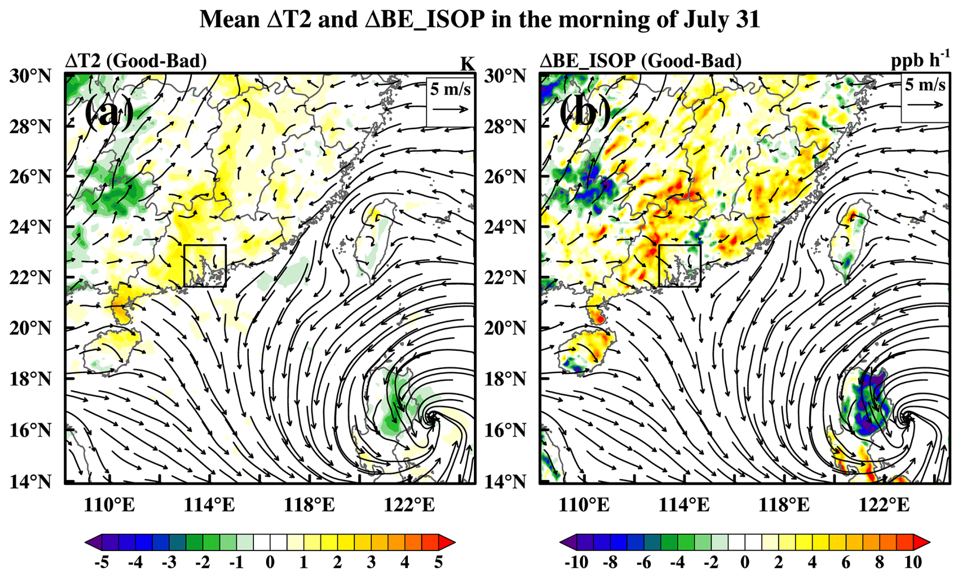
Figure 10 Mean distributions of ΔT2 (a) and ΔBE_ISOP (b) between good and bad EMs (good − bad) during the morning (09:00–12:00 LT) of 31 July.

3.3 Source apportionment of extremely high ozone concentrations

With the implementation of the ozone source apportionment method, the contributions of ozone from various geographical source regions on 31 July were quantified. As illustrated in Fig. 11a, the local area made the greatest contribution to surface in the GBA during the daytime. Especially during the high-ozone period (11:00–16:00 LT), the mean local contribution could reach 65.4 ppb. In addition to the GBA, the surrounding areas (i.e., WGD) and the remote source region (i.e., SEASIA) showed obvious ozone contributions (with mean contributions of 4.0 and 6.8 ppb, respectively) during this period. In addition, INIT2 and INFLOW, which derived from the initial and boundary conditions of chemistry, also contributed to the surface ozone in the GBA.

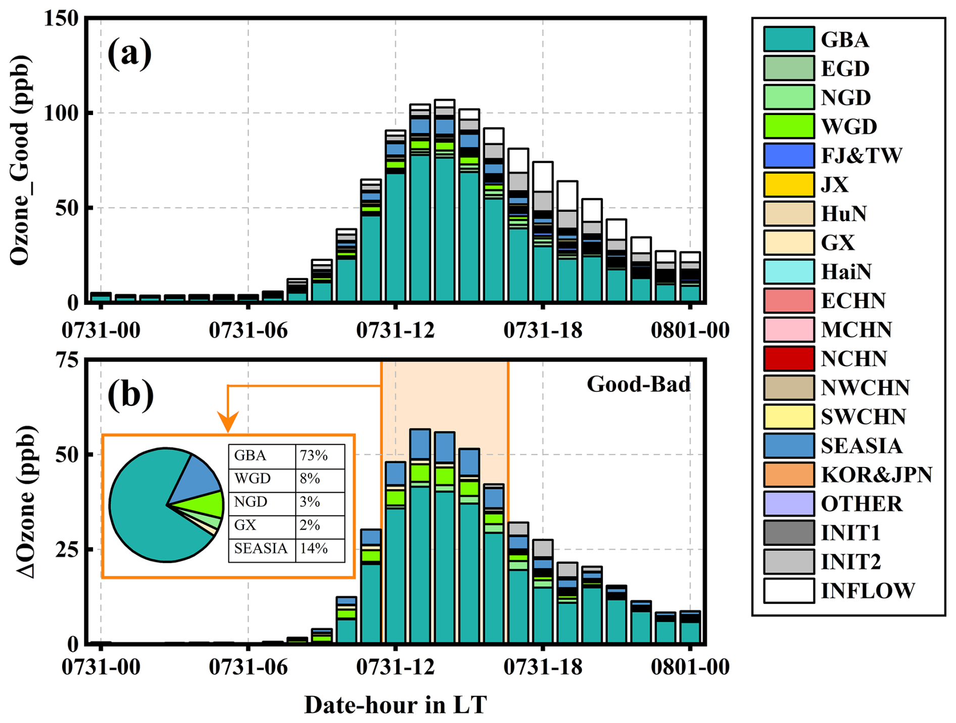
Figure 11 Mean surface ozone contributions of good EMs (a) and mean changes in surface ozone contributions between the good and bad EMs (b) in the GBA on 31 July.

By comparison with the bad EMs (Fig. 11b), the changes in ozone contributions were quantified, which could be used to determine the primary contributors to the increase in ozone during the daytime on 31 July. It is clear that ozone contributions from the local region (GBA), surrounding regions (WGD, NGD, and GX), and remote regions to the west (SEASIA) increased on 31 July. During the period from 11:00 to 16:00 LT, their respective proportions in the ozone increase accounted for 73 %, 8 %, 3 %, 2 %, and 14 %. In terms of local contribution, the GBA was controlled by stagnant weather, which was not favorable for the diffusion of atmospheric pollutants. As a result, ozone precursors accumulated locally and produced more ozone through photochemical reactions. As shown in Fig. 10b, WGD, NGD, and GX were controlled by westerly winds during the morning of 31 July. Considering the greater amount of BVOCs emitted into the atmosphere over these regions, more ozone and its precursors might be transported and contribute to the increase in surface ozone in the GBA. Our results are consistent with those of previous studies in this region (Li et al., 2012, 2022; Wang et al., 2022).

As a remote source region, the ozone contribution from SEASIA also significantly increased on 31 July. However, unlike the local and surrounding regions, ozone and its precursors from SEASIA are challenging to transport to the GBA at ground level or low altitudes due to dry/wet deposition and chemical consumptions, suggesting a reliance on higher transport pathways. Based on the vertical cross section of the ozone contribution from SEASIA along the west–east direction (Fig. 11), the high-concentration zone was located to the west of the GBA. Under the control of westerly winds, ozone from SEASIA could be transported to high altitudes in the area. Notably, due to the low wind speeds over the GBA, high ozone concentrations from SEASIA were confined to the residual layer in the early morning (Fig. 12a). When the PBL developed, the ozone aloft began to be entrained downward (Fig. 12b). With the continuous rise of the PBL, ozone aloft continued to be transported to the surface through vertical mixing, ultimately contributing to the increase in surface ozone (Fig. 12c). This finding aligns with the physical cause of the high ozone concentration we discussed in Sect. 3.2.2.

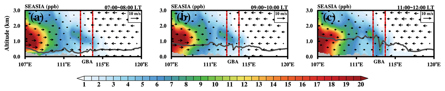
Figure 12 Mean vertical cross sections of the ozone contribution from SEASIA along the west–east direction during the morning on 31 July. (a) 07:00–08:00 LT, (b) 09:00–10:00 LT, and (c) 11:00–12:00 LT.

4 Conclusion

Extremely high ozone episodes may occur in the GBA when typhoons approach South China. Notably, numerical models often struggle to accurately reproduce the high concentrations of ozone during these episodes, which complicates the study of their formation mechanisms. Additionally, this type of ozone pollution is influenced by the competing effects between typhoon and WPSH. Significant errors may arise when investigating its formation by comparing base and sensitive experiments (keeping and erasing typhoon system).

In this study, we took an extremely high ozone episode that occurred in the GBA in the summer of 2016 as a case study for numerical analysis. This ozone episode occurred when Typhoon Nida approached. The observations revealed that the maximum concentration reached as high as 366 µg m⁻³ in the afternoon of 31 July. To more accurately capture the pollution characteristics, we conducted an ensemble simulation using the WRF-Chem-O3tag model. By using R and MNB, we introduced an index, I_dis, to select good and bad EMs. Through model validation, the good EMs exhibited a better model performance in capturing the characteristics of the high-ozone episode, including both the high concentrations and the variation patterns, compared to the bad EMs.

By comparing the good and bad EMs, we quantitatively examined the physical and chemical causes of the extremely high concentrations and the ozone contributions from various geographical source regions in this study. The extremely high ozone concentration could be explained from both physical and chemical perspectives. From a physical perspective, the GBA experienced weak winds as Typhoon Nida approached. Weak winds facilitated a more significant accumulation of ozone in the residual layer during the evening and early morning. When the PBL developed in the morning, ozone aloft was continuously entrained downward to the surface and then significantly contributed to surface ozone. From a chemical perspective, the approach of typhoon provided favorable meteorological conditions for ozone photochemistry, such as increased temperature and more solar irradiance. However, our results revealed that the photochemical reaction constants (i.e., photolysis rate) changed only slightly during the high-ozone period. More importantly, weak winds contributed to the accumulation of ozone precursors in the GBA. The increased ozone precursors were the primary reason for the dramatic enhancement of photochemistry. In addition, the increased temperature could increase the concentration of biogenic VOCs by intensifying biogenic emissions from vegetation. The increase in biogenic VOCs could also significantly contribute to the increase in ozone precursors.

The ozone source apportionment results in the good EMs revealed that ozone from the local source region (GBA) contributed most significantly to the high-ozone episode. Furthermore, the surrounding regions (i.e., WGD) and remote regions (i.e., SEASIA) also made significant contributions. During the high-concentration period on 31 July, the mean ozone contributions from the GBA, WGD, and SEASIA were 65.4, 4.0, and 6.8 ppb, respectively. Compared to the bad EMs, the ozone contributions from the GBA, WGD, NGD and GX significantly increased, which was primarily caused by stagnant weather in the GBA and westerly transport effects from outside the area. In addition, ozone from the western and remote region (SEASIA) could be transported to the GBA via westerly winds at high altitudes. When the PBL developed in the morning, ozone aloft was entrained downward, significantly contributing to the surface ozone in the GBA.

The methods employed in this study provide an efficient way to enhance model performance for the extremely high ozone episodes that occurred in the GBA before the landfall of typhoons. Through the comparisons between good and bad EMs, our findings can offer clear insights into the formation and source contributions of such ozone pollution. It is important to note that the changes in ozone between good and bad EMs originated from the discrepancies in the meteorological fields in this study. Consequently, despite the model performance having improved, the simulated ozone of good EMs still showed differences from the observed ozone. We believe that integrating the impacts of anthropogenic emissions could further enhance model performance in ozone simulation, which we will address in our future research.