Soil deposition of atmospheric hydrogen constrained using planetary-scale observations

Quantifying soil deposition fluxes remains the greatest source of uncertainty in the atmospheric H₂ budget. A new method is presented to constrain H₂ deposition schemes in global models using observations of the zonal mean H₂ distribution and seasonality. A “best-fit” scheme that reproduces the observed zonal-mean seasonality of atmospheric H₂ at the planetary scale is found by perturbing a prototype deposition scheme based on soil temperature and moisture dynamics. Comparing the best-fit and prototype schemes provides insight into how the prototype scheme may be improved to better reproduce observed seasonality. The H₂ signal driven by the prototype scheme is accurate compared to observations in the Northern Hemisphere extratropics but shows discrepancies in the Southern Hemisphere, with surface mixing ratios that are too high and seasonality that is too weak. A best-fit scheme indicates that the function capturing the soil microbial consumption of H₂ requires a shift of +2 to +3 months in the seasonality in the tropics, with peak uptake shifting from February to April in the southern tropics and from August to October in the northern tropics, compared with a prototype scheme sensitive to seasonal soil moisture driven by the shifting of the Intertropical Convergence Zone. New constraints on the H₂ surface flux at low latitudes are key to accurately modelling the H₂ cycle in the Southern Hemisphere.

1 Introduction

In recent years, there have been widespread announcements of new plans for hydrogen energy systems (Warwick et al., 2023). As such, future hydrogen emissions are expected to increase, largely due to fugitive emissions from infrastructure (Ocko and Hamburg, 2022; Esquivel-Elizondo et al., 2023). Although the symmetrical H₂ molecule is not itself a greenhouse gas, its presence depletes atmospheric OH that would otherwise oxidise methane (Warwick et al., 2023). Hydrogen oxidation by OH additionally contributes to the formation of the greenhouse gases ozone and water, with the latter having a significant warming effect in the otherwise dry stratosphere (Sand et al., 2023; Warwick et al., 2023). However, despite the increasing number of modelling studies that have provided new insights into the atmospheric chemistry of H₂, there remain large uncertainties in evaluations of the global warming potential (GWP) of H₂ (Sand et al., 2023; Derwent, 2023). Different recent estimates for the GWP over a 100- year time horizon include: Sand et al. (2023), 11.6 ± 2.8; Derwent (2023), 7.1–9.3; and Warwick et al. (2023), 12 ± 6. Quantifying the soil sink and counterbalancing H₂ emissions have remained the main source of uncertainty in the atmospheric H₂ budget (cf. Novelli, 1999; Sand et al., 2023), and hence the lifetime of H₂, which generates large uncertainty in the GWP calculations that are relied on for understanding the climate impacts of H₂ applications.

Present-day (2010s) surface H₂ mixing ratios are ca. 550 ppb (Pétron et al., 2023), having increased at a rate of about 2.5 ppb yr⁻¹ in the latter part of the 20th century (Patterson et al., 2020). Multi-decadal increases in H₂ can mainly be attributed to increases in methane oxidation, while sub-decadal variations are more related to changes in the soil sink and H₂ emissions (Derwent et al., 2023; Paulot et al., 2024). H₂ concentrations show a distinct latitudinal variation, with values about 50 ppb higher in the Southern Hemisphere (SH) compared to the high latitudes of the Northern Hemisphere (NH). They also show a characteristic seasonal cycle; outside the tropics, H₂ generally peaks in the summer, with a monthly mean peak-to-peak magnitude of 30–60 ppb in the NH and 15–30 ppb in the SH.

To produce the same observed atmospheric H₂ concentrations, a stronger soil sink implies greater emissions and a shorter atmospheric lifetime (Hauglustaine et al., 2022; Ehhalt and Rohrer, 2013; Sand et al., 2023). In a comparison of six atmospheric chemistry models with imposed boundary layer H₂ concentrations, Sand et al. (2023) evaluated an uncertainty contribution to the GWP of 18 % of the mean, due to uncertainty in the soil sink.

While constraining the annual mean planetary soil sink helps constrain the lifetime of H₂ in the bulk atmosphere, the observational data contain additional useful information about the latitudinal distribution and seasonal variation of H₂ that we exploit here. We filter these observations to decompose the observed H₂ signal into a 2012–2018 mean background state and a seasonal cycle (Sect. 3).

Several different deposition schemes to model the soil sink of H₂ exist (e.g. Sanderson et al., 2003; Paulot et al., 2021; Ehhalt and Rohrer, 2013; Bertagni et al., 2021). These schemes are typically based on laboratory or field studies of a small number of deposition flux samples (e.g. Yonemura et al., 2000; Meredith et al., 2017) and model deposition velocities with functions of soil texture, water content, and temperature. There are also indications that soil carbon content is important in determining the H₂ deposition velocity (Khdhiri et al., 2015; Karbin et al., 2024). Here we provide a method to evaluate deposition schemes at the planetary scale. Observational data from surface H₂ measurements provide time series of surface mixing ratios from a globally distributed set of sites (Pétron et al., 2023). We extend previous analysis of the seasonality of individual station measurements (Novelli, 1999) and the combined roles of tropical biomass burning, deposition, and convective uplift in contributing to seasonal variation (Hauglustaine and Ehhalt, 2002; Yashiro et al., 2011), through an analysis that accounts for the continuous variation of seasonality with latitude. This extends the work of Xiao et al. (2007) in spatial and temporal resolution, who have previously decomposed H₂ sources and sinks based on the seasonality in tropical and extratropical regions.

Our results and analysis also complement Paulot et al. (2024), who have revised H₂ emissions and deposition estimates to better reproduce the H₂ distribution and seasonality of clustered observations. They identified major gaps in our understanding of the soil removal of H₂. We analyse the soil uptake arising from a model constrained to reproduce a latitude-varying H₂ seasonality, while relaxing assumptions about the estimated soil uptake.

The annual mean distribution and seasonality of H₂ concentration are controlled by surface emissions and deposition, by production and loss by atmospheric chemistry, and by atmospheric transport. Due to the slow response of relatively well-mixed H₂ in the atmosphere, with a lifetime ∼ 2 years (see Ehhalt and Rohrer, 2009; Patterson et al., 2020; Warwick et al., 2023; Sand et al., 2023), we assume that the general effect of these fluxes is well approximated when they are modelled in their zonal-mean monthly-mean.

We first introduce a prototype deposition scheme based on formulations of the moisture and temperature dependence of soil biology and diffusion processes (Sect. 2). Then we provide a new analysis of the observed H₂ distribution and seasonality (Sect. 3). We include the prototype deposition scheme in a toolbox model (Sect. 4) with estimates of emissions with a spatial and monthly signal from Paulot et al. (2021), together with emission strength and atmospheric chemical production and destruction fluxes from Sand et al. (2023), and tropospheric transport, idealised as a latitude–height overturning from ERA5 monthly mean wind speeds (Hersbach et al., 2020), and atmospheric dispersion parameters tuned based on reproducing the observed SF₆ distribution. By comparing the simulated H₂ concentration against the observed distribution and seasonality, we determine new constraints on soil deposition as a function of latitude, which we apply to tune the original prototype scheme (Sect. 5).

2 A prototype deposition scheme

H₂ oxidising bacteria are ubiquitously distributed in soils (Schlegel, 1974; Khdhiri et al., 2015; Greening et al., 2016; Ji et al., 2017; Bay et al., 2021; Greening and Grinter, 2022).

Recently, Bertagni et al. (2021) formulated the uptake of atmospheric H₂ – constrained by the rate of gas diffusion into soil and its microbial activity – as functions of soil type, temperature, and moisture, and without including a function of soil carbon, to derive a global model for H₂ deposition.

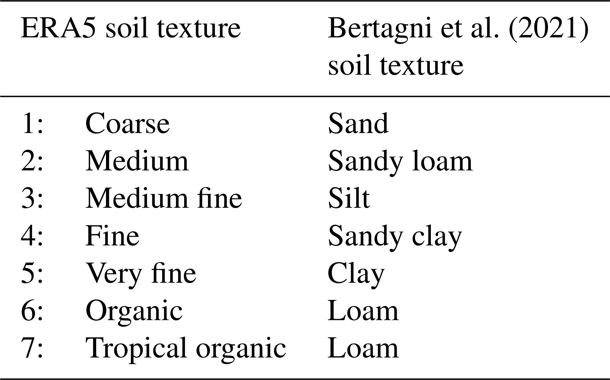
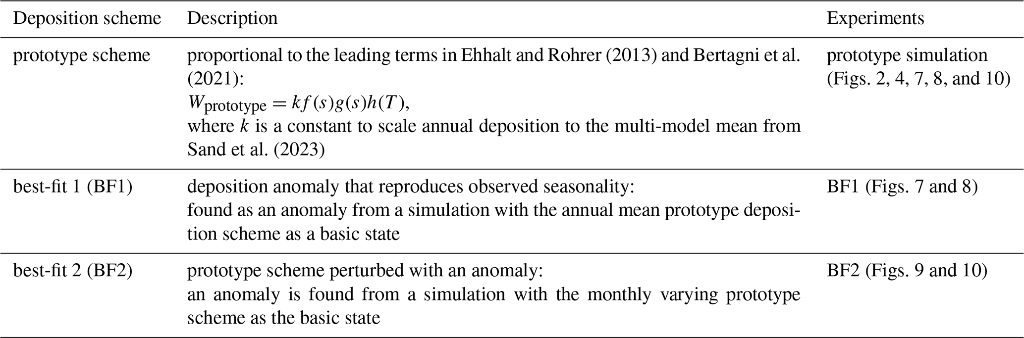
To simplify our analysis of the dominant drivers of seasonality in H₂ deposition, we implement a prototype scheme that isolates the deposition rate seasonality due to terms limited by soil moisture, s, proportional to f(s) and g(s) and by soil temperature, T, proportional to h(T) (Ehhalt and Rohrer, 2011; Ehhalt and Rohrer, 2013; Bertagni et al., 2021). The terms f(s) and h(T) limit potential microbial activity, and g(s) models the gas diffusivity into the soil. Ehhalt and Rohrer (2013) and Bertagni et al. (2021) identified the importance of high-frequency fluctuations in their deposition models – particularly as a product of the changing soil moisture depth profile through cycles of precipitation and drying. As we base our constraints on the planetary-scale seasonality at lower frequencies of 1–2 yr⁻¹, we drive f, g, and h with monthly mean ERA5 soil moisture in the top 7 cm and skin temperature and scale the deposition rate with a constant to close the H₂ budget, as in Sand et al. (2023) (summarised in Table 3). A comparison of f and g with soil moisture varying on 30 d and daily timescales is provided in Fig. A1. The use of monthly average ERA5 data can lead to slightly faster uptake rates in semi-arid regions (cf. Bertagni et al., 2021) but does not substantially affect the seasonality.

Bertagni et al. (2021)

Table 1 Mapping of ERA5 soil textures to the Bertagni et al. (2021) soil parameters. The medium and medium fine textures dominate over the land surface.

Analytically, the resultant H₂ uptake is the parallel sum of the potential flux limited by biological activity and the potential flux limited by diffusion (Bertagni et al., 2021). However, that formulation would require accurate quantification of each flux. Alternatively, Ehhalt and Rohrer (2013) have formulated deposition velocity in moist soils to vary with $(fgh{)}^{\mathrm{1}/\mathrm{2}}$. However, in this work, the objective of the prototype scheme is to capture the seasonality in these processes while facilitating an analysis of how these processes drive the planetary H₂ distribution. Therefore, we adopt an idealised formulation where the total uptake is proportional to the product of the normalised terms, fgh, and is scaled to achieve a total 57.2 Tg yr⁻¹ average deposition (following Sand et al., 2023).

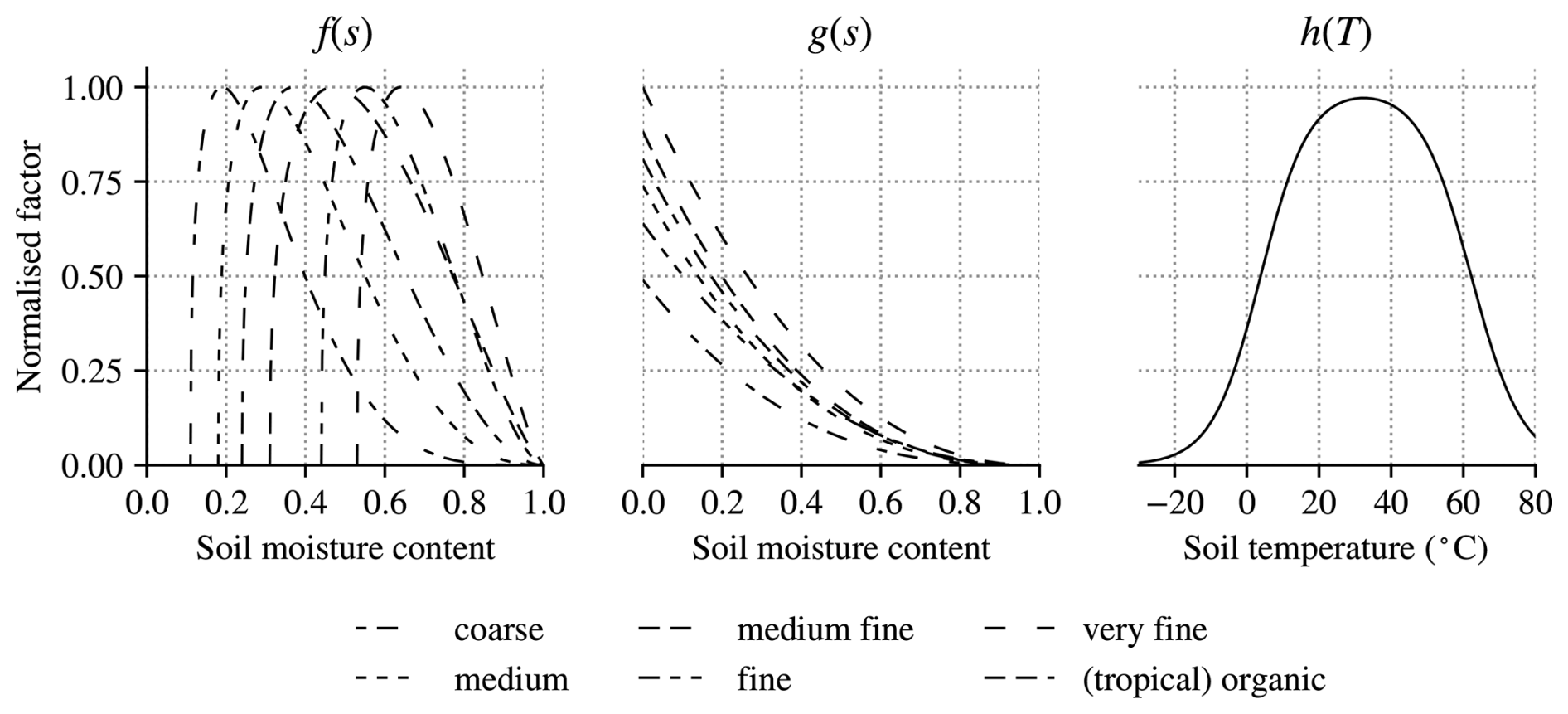
Figure 1 Normalised soil deposition rate factors (sourced from Ehhalt and Rohrer, 2011, Bertagni et al., 2021): (a) f and (b) g for different soil textures used in ERA5 (Table 1); and (c) h.

Suppressed H₂ uptake has been measured in soils at low and high moisture contents (Conrad and Seiler, 1981), yet Bertagni et al. (2021) emphasise the continued lack of quantitative observations on how soil biological activity varies with soil moisture. In lieu of these data, they provide an adaptable model that constrains the soil moisture-limiting function with the soil matric potential for different soil textures. Accepting this persistent difficulty, we define f(s) (Fig. 1a) as a mapping of that defined function to the ERA5 set of soil textures (Table 1).

Bertagni et al. (2021) identify the importance of a diffusive limitation on H₂ deposition in humid regions. They model the H₂ flux into the soil as proportional to the parallel addition of the gas conductance of the diffusive soil layer, g, and the gas conductance of any diffusive barrier – such as organic litter or snow cover. They adopt the soil structure-dependent gas diffusivity model of Moldrup et al. (2013) from which we propose an idealised moisture-dependent gas conductivity for H₂ into soil, assuming a constant free-air diffusion rate and a diffusive-layer length scale,

$$\begin{array}{}\text{(1)}& g\left(s\right)\propto n^{\mathrm{2}}(\mathrm{1}-s{)}^{\mathrm{2}+\frac{\mathrm{3}}{b}}\end{array}$$

where the soil porosity n and the parameter b are compiled for different soil textures in Bertagni et al. (2021). The resulting normalised g is plotted in Fig. 1b.

The effects of diffusive barriers are diagnosed by Bertagni et al. (2021). Their presence has the strongest limiting effect where the underlying soil diffusivity is highest, but this is masked where biological uptake is strongly limited due to lack of soil moisture or by cold temperatures where there is snow cover. Therefore, rather than relying on broad assumptions for the distribution of diffusive barriers, in our prototype scheme we assume a total gas diffusivity proportional to g.

We choose h(T) as the normalised soil temperature dependence across H₂ removal experiments that was defined by Ehhalt and Rohrer (2011) (Fig. 1c), where H₂ removal occurs from temperatures as low as −20 °C, increases following a Fermi distribution to a peak at around 30 °C (cf. Smith-Downey et al., 2006), and is quickly limited for temperatures higher than 40 °C.

3 Filtering and decomposition of H₂ observations

Time series of H₂ mixing ratios (Pétron et al., 2023) have been measured at the NOAA Global Monitoring Laboratory using flask samples received from a latitude-spanning network of sites (NOAA Global Monitoring Laboratory, 2024). These flask samples have typically been taken once or twice weekly since 2010 (Pétron et al., 2023) using a portable sampling unit with a ca. 5 m mast, and samplers are instructed to preferably sample upwind of buildings at times when wind speeds are ≥ 2 m s⁻¹ (NOAA Global Monitoring Laboratory, 2005).

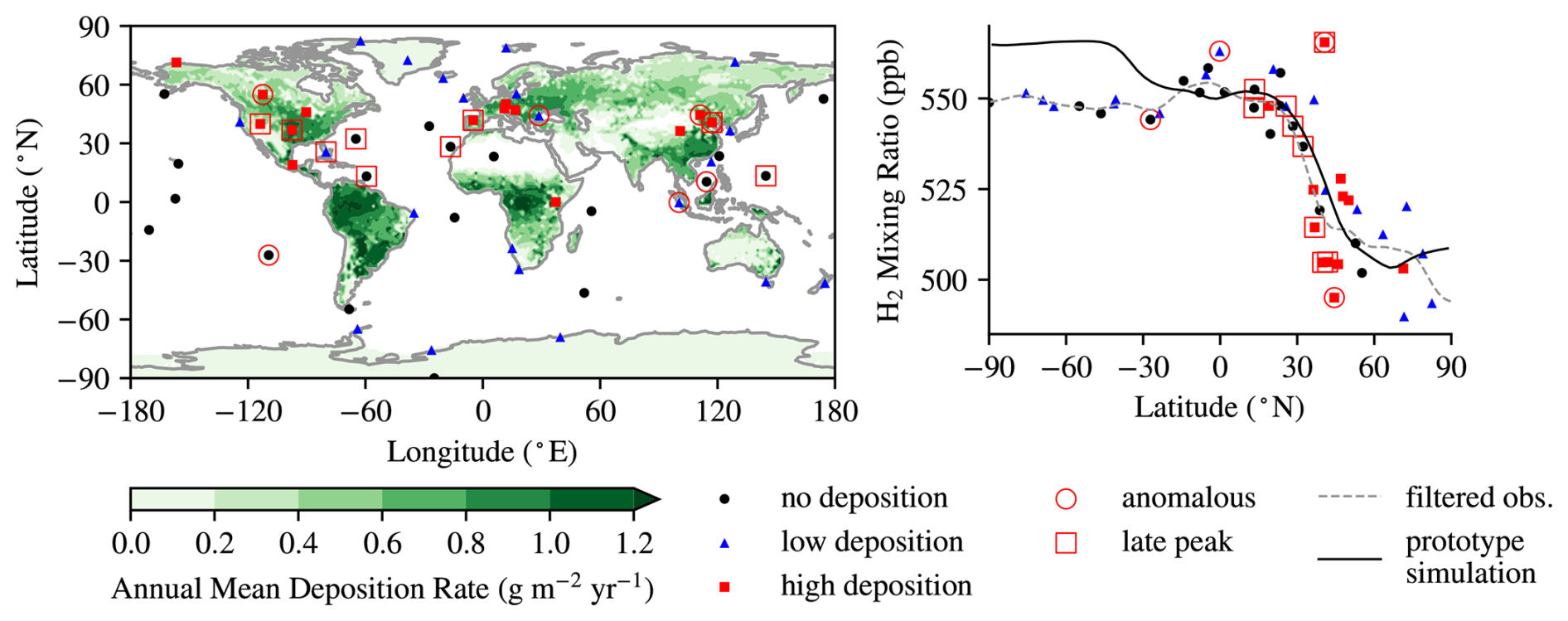
Figure 2 (a) Annual mean H₂ deposition flux ($\mathrm{g}{\mathrm{m}}^{-\mathrm{2}}{\mathrm{yr}}^{-\mathrm{1}}$) in the prototype deposition scheme (shading), with surface H₂ measuring stations (symbols) (NOAA Global Monitoring Laboratory, 2024) filtered by local deposition in the prototype deposition scheme (Table 2). (b) Observed 2012–2018 mean H₂ mixing ratio at surface measuring sites (symbols, labelled according to the average prototype deposition within ± 2.5° N and ± 2.5° E: no deposition; low deposition $\in (\mathrm{0},\mathrm{0.2}]$ $\mathrm{g}{\mathrm{m}}^{-\mathrm{2}}{\mathrm{yr}}^{-\mathrm{1}}$; and high deposition > 0.2 $\mathrm{g}{\mathrm{m}}^{-\mathrm{2}}{\mathrm{yr}}^{-\mathrm{1}}$) (Pétron et al., 2023) and the near-surface zonal model results from a simulation using the prototype deposition scheme (solid line). Anomalous sites (circled) are identified following Eq. (B1). A cluster of sites in the NH subtropics has a peak in the first harmonic after 150 d (squared, in Fig. 4 peak 1–2 months later than other sites in the subtropics). Filtered observations (grey dashed line) are a fit to the observational data excluding anomalous stations (circled) using a Gaussian filter with σ = 5° lat. Plotted station data are summarised in Table C1.

Ehhalt and Rohrer (2013)Bertagni et al. (2021)Sand et al. (2023)

Table 2 Summary of deposition schemes used and devised in this study.

We apply spatial filtering to the measurement sites based on the predicted annual mean deposition rate in the biophysics-based prototype deposition scheme that we introduce in Sect. 2 (Fig. 2a). By drawing a systematic comparison across sites, we are able to extract general features of the planetary signal of background surface H₂ distribution and seasonality.

In addition to the spatial filtering of sites, temporal filtering is used to decompose how the observed H₂ signal varies over different timescales. We analyse the seasonality at each site, then compare these signals across latitudes rather than finding the seasonality of latitude-clustered sites (cf. Paulot et al., 2024), restricting our analysis to a set of station measurements where consistent sampling exists during the period 2012–2018.

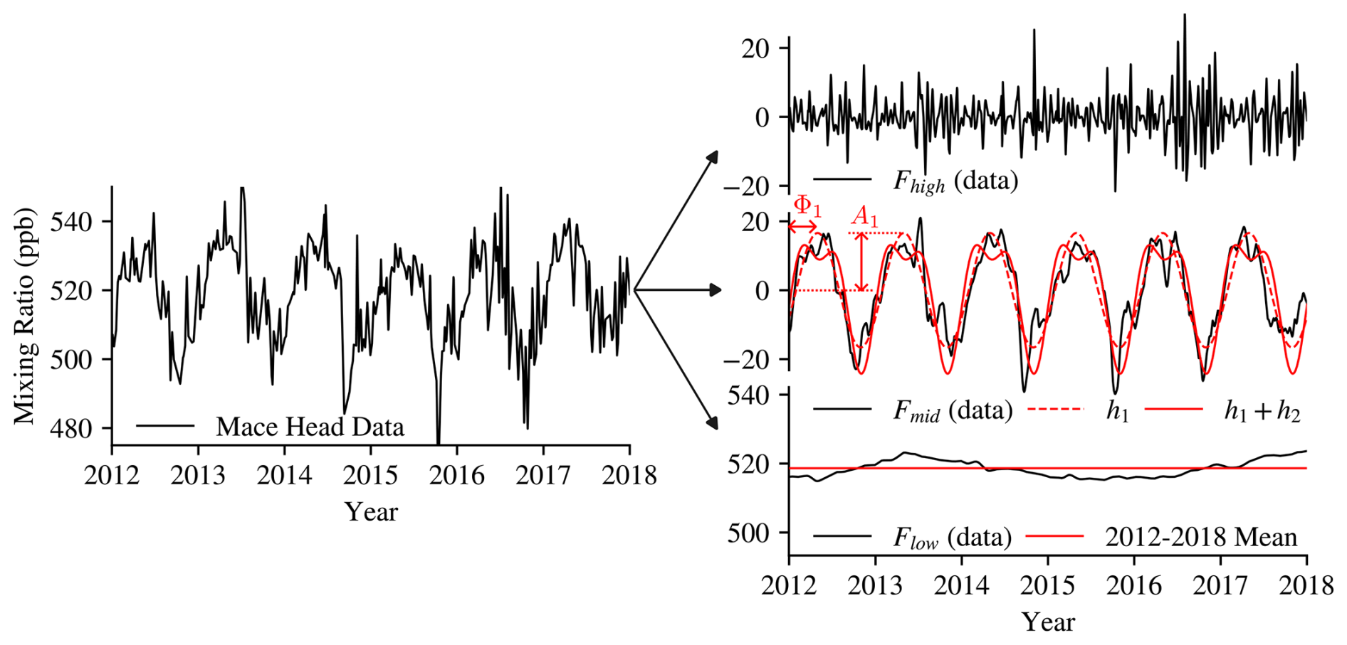
Figure 3 Example decomposition of the 2012–2018 H₂ observations from the Mace Head atmospheric research station (left) (Pétron et al., 2023) into: top-right, high-frequency noise on timescales < 30 d (F_high); mid-right, seasonality on timescales 30 d–1 year (F_mid), with the first (h₁) and second (h₂) harmonics fitted to this (red solid and dashed lines, respectively); bottom-right, the residual inter-annual variation (F_low); and the 2012–2018 mean (red line). The amplitude, A₁, and phase, Φ₁, of the first harmonic are indicated.

We implement a filter, F_mid, to isolate the seasonal cycle. F_mid returns the recorded data minus the high-frequency noise isolated with a high-pass filter, F_high, and the interannual variation isolated with a low-pass filter, F_low. This decomposition is illustrated for data recorded at the Mace Head atmospheric research station in Fig. 3. High-frequency noise driven by synoptic weather occurs on timescales < 30 d and is isolated with F_high by subtracting a central moving average with a 30 d window from the data. Subtracting the high-frequency noise from the data reveals a background state where the remaining temporal variation is dominated by a seasonal cycle (Paulot et al., 2024). Therefore, to isolate the low-frequency interannual variability and trends, it is suitable to define F_low as a central moving average with a 1-year window.

This background state reveals the trend of increasing atmospheric burden, varying on timescales τ_low ≥ 1 year (Novelli, 1999; Patterson et al., 2020; Ehhalt and Rohrer, 2013). Furthermore, the meridional gradient of its mean state (Fig. 2b), combined with quantification of the atmospheric chemical production and loss of H₂, reveals the net surface fluxes in either hemisphere (Sanderson et al., 2003).

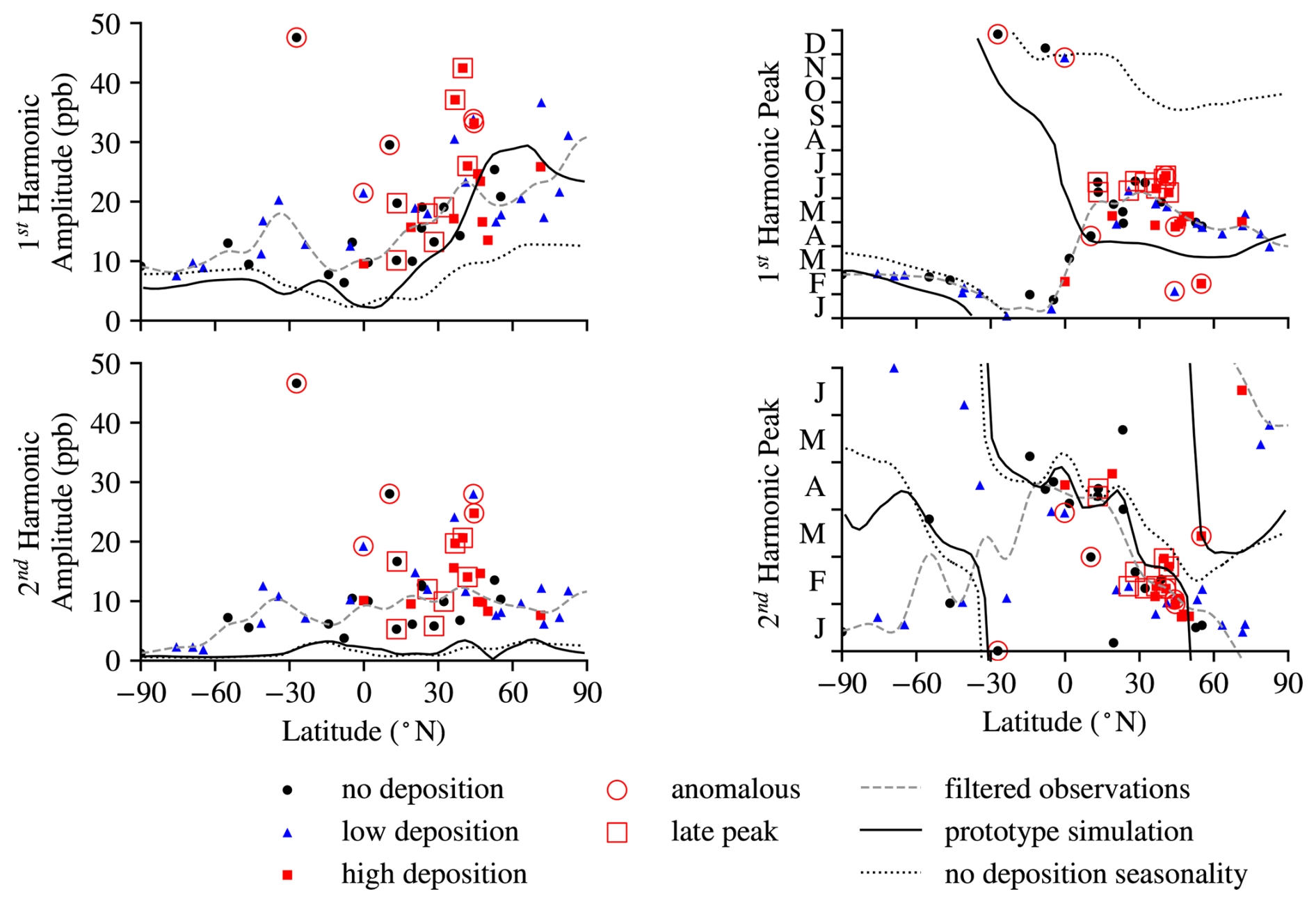
Figure 4 Seasonality of the 2012–2018 H₂ mixing ratio at surface measuring sites (symbols, see Fig. 2) (Pétron et al., 2023), the near-surface conditions of a simulation using the prototype deposition scheme (solid line, see Table 2) and using the annual mean deposition velocity of this scheme (dotted line): (a) and (c) the amplitudes of the first and second harmonics of the seasonal oscillation (A₁ and A₂); and (b) and (d) the phase of the peak of the first and second harmonics of the seasonal oscillation (Φ₁ and Φ₂). Note, the pattern for Φ₂ over the first 6 months repeats over the last 6 months. Filtered observations (grey dashed line) is a fit to the observational data excluding anomalous stations using a Gaussian filter with σ = 5° lat.

The first harmonic of the seasonality at each site (Fig. 4a and b) is identified by optimising the fit of the curve

$$\begin{array}{}\text{(2)}& h_{\mathrm{1}}(A_{\mathrm{1}},{\mathrm{\Phi }}_{\mathrm{1}})=A_{\mathrm{1}}\cos \left(\mathrm{\Omega }\right(t-{\mathrm{\Phi }}_{\mathrm{1}}\left)\right)\end{array}$$

to the F_mid filtered data, where A₁ and Φ₁ are, respectively, the amplitude and phase of the harmonic (illustrated for Mace Head in Fig. 3), and Ω = 2 π yr⁻¹. Additionally, a second harmonic of the seasonality is identified by optimising the fit of

$$\begin{array}{}\text{(3)}& h_{\mathrm{2}}(A_{\mathrm{2}},{\mathrm{\Phi }}_{\mathrm{2}})=A_{\mathrm{2}}\cos \left(\mathrm{2}\mathrm{\Omega }\right(t-{\mathrm{\Phi }}_{\mathrm{2}}\left)\right)\end{array}$$

to the F_mid filtered data minus h₁ (Fig. 4c and d).

The accuracy of describing the seasonality with $A_{\mathrm{1}},{\mathrm{\Phi }}_{\mathrm{1}},A_{\mathrm{2}},{\mathrm{\Phi }}_{\mathrm{2}}$ at each site is assessed by considering the root mean square (RMS) error of h₁+h₂ minus the F_mid filtered data. Anomalous results are categorised where this RMS error is greater than 20 ppb (Eq. B1, sites indicated in Fig.2). By inspection, this criterion effectively excludes five sites where harmonics could not be identified (such as in Fig. 3).

Between 2012 and 2018, both the annual mean surface H₂ mixing ratio (Fig. 2b) as well as the amplitude (Fig. 4a) and phase (Fig. 4b) of the seasonal variability – the time of the peak of the first harmonic of the seasonal variability – are well described by a function of latitude. A Gaussian filter with a standard deviation of 5° latitude is used to find a best fit between observations, excluding anomalous sites. The small spread of the phase of the seasonality of H₂ observations from the best fit shows that the mid-filtered signal varies more with the latitude of sites than with zonal variations in local deposition. We exploit an H₂ seasonality that continuously varies with latitude as a distinct constraint, in contrast to Paulot et al. (2024). This constraint allows us to test assumptions in the prototype deposition scheme at higher meridional resolution (Sect. 5).

Neglecting the trend of increasing H₂ concentrations – which are propagated to the planetary scale due to its long atmospheric lifetime – and considering the dominant role of surface uptake in the H₂ sink, this meridional gradient (Fig. 2b) suggests net down-gradient mixing from the tropics to the NH high latitudes, in contrast to approximately no meridional gradient between the tropics and SH mid- and high latitudes. This supports the assumption that the deposition into soils is dominated by the larger land area of the NH, where this soil sink exceeds anthropogenic emissions and the net source of H₂ from atmospheric chemistry (Paulot et al., 2021).

Outside the tropics, the first harmonic of the seasonal oscillation peaks in the late spring to early summer – between April and June – in the NH, and in late summer – late February – in the SH (Fig. 4b). The amplitude of this harmonic increases with latitude in the NH and is reduced in the deep tropics compared with the subtropics, reflecting the different seasonality in the tropics compared with temperate regions (Fig. 4a). Figure 4b shows a spread in the phase of the seasonality in the NH between 10 and 45° N of about 2 months, from late April to late June. There is a cluster of measurements where the first harmonic peaks in June – later in summer in the NH, more similar to the late summer peak in the SH (red squares, Figs. 2 and 4). These sites are spread zonally and have an amplitude of the first harmonic as well as a second harmonic of seasonality, consistent with other observations in the NH (Fig. 4a, c, and d).

We define a reference monthly mean H₂ mixing ratio, r_ref, as the sum of the observed annual mean state and the first and second harmonics fit to the observations with a Gaussian filter with σ = 5° lat, excluding stations with anomalous signals. The width of the filter was chosen to produce a smooth best fit to observations that preserves the distinct patterns with latitude that vary over scales ca. 10° N. This reference H₂ signal isolates the dominant signal from noise and inter-annual variability, and the decomposition of r_ref recovers the best-fit to the 2012–2018 surface observations: in the annual mean (grey dashed, Fig. 2b); the first harmonic of the seasonality (grey dashed, Fig. 4a and b); and the second harmonic (grey dashed, Fig. 4c and d).

The importance of deposition seasonality is indicated in Fig. 4: a simulation with the same annual deposition flux but without deposition seasonality (dotted line) fails to reproduce key features of the planetary H₂ seasonality. In the simulation with H₂ seasonality driven by emissions, deposition, and atmospheric chemistry (solid line), in both hemispheres, H₂ peaks in late summer to early autumn, February–March in SH, and August–September in NH, with a similar zonal-mean peak amplitude of 10–15 ppb to the observations in the mid-latitudes. Seasonally varying deposition is required for NH H₂ to peak earlier in the year and to resolve the distinct latitude bands of peak seasonality. Alternatively, prototype deposition seasonality has little impact in the SH due to the relative lack of land. In the SH, the seasonality of H₂ is mainly controlled by atmospheric chemistry.

4 Model formulation

Analysis of the 2012–2018 observational data for H₂ mixing ratio (from Pétron et al., 2023) showed that the mean and first and second annual harmonics of the H₂ distribution (Figs. 2b and 4a–d) are well described by a function of latitude. Additionally, we note the long average lifetime of H₂ compared with timescales of horizontal mixing in the atmosphere (e.g. Pierrehumbert and Yang, 1993), indicating that H₂ is reasonably well mixed across zonal bands. However, this assumption is challenged at latitudes with particularly strong sources and sinks. For example, there is a spread of ca. 5 % in the non-anomalous observed annual mean mixing ratios around 40° N (Fig. 2b).

Therefore, we attempt to simulate a planetary H₂ signal in a simple 2D (latitude–height) model with monthly varying zonal-mean emissions, atmospheric loss and production, soil deposition, and transport integrated with a fourth-order Runge–Kutta method, with 30 d months and 4 steps per day. The latitude–height model comprises 64 equally spaced latitude bands with three layers representing the lower, middle, and upper troposphere, for which we assume fixed pressure boundaries at 1000, 800, 600, and 150 hPa. The simplicity of the model is prioritised such that simulations carry a low computational cost and differences resulting from the model configurations may be readily identified.

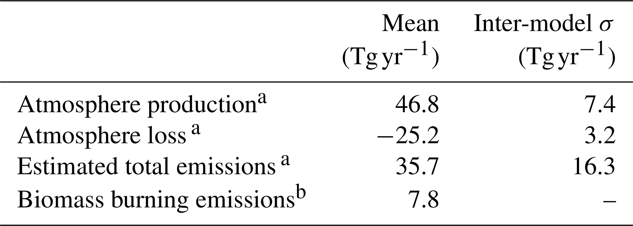
Table 3 Summary of annual mean H₂ fluxes input to the model from: ^a Sand et al. (2023) mean over six fixed boundary layer concentration-driven models with estimated emissions and the standard deviation across the six models. ^b The emissions from biomass burning of the total emissions from Marle et al. (2017).

4.1 Emissions of H₂

We constrain the total H₂ emissions and production and destruction by atmospheric chemistry to match the multi-model average flux estimates in Sand et al. (2023) from six models driven by prescribed boundary layer H₂ and CH₄ concentrations (summarised in Table 3). In Sand et al. (2023), total H₂ emissions were estimated as the residual in offline calculations considering simulated atmospheric H₂ production and destruction and estimated H₂ deposition. They found an inter-model mean of 35.7 ± 16.3 Tg yr⁻¹ (summarised in Table 3 from Sand et al., 2023), which corresponds to the estimate of the 1995–2015 average H₂ emissions of Paulot et al. (2021): 29.9–37.1 Tg yr⁻¹.

We set annual H₂ emissions to 35.7 ± 16.3 Tg, of which 7.8 Tg are monthly varying biomass burning emissions based on the input4MIPs estimate (Marle et al., 2017). The remaining emissions from anthropogenic sources and nitrogen fixing are implemented using the monthly mean signals from Paulot et al. (2021) in their respective proportions but requiring a ca. +20 % scaling: 17.1 and 10.8 Tg, respectively. The seasonality and latitudinal distribution of emissions are shown in Fig. 5a and b.

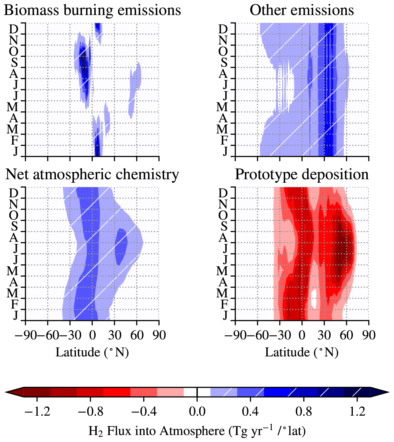
Figure 5 H₂ fluxes in the model: (a) emissions from biomass burning (from Marle et al., 2017); (b) other emissions including combustion of fossil fuels and nitrogen fixing in soils and oceans (based on Paulot et al., 2021; Sand et al., 2023); (c) net production minus destruction by atmospheric chemistry (from Sand et al., 2023); and (d) zonal-mean deposition with the prototype scheme.

4.2 Atmospheric chemistry of H₂

As shown in Figs. 2b and 4, the prototype simulation (black line) captures much of the observed H₂ distribution and seasonal variation (symbols) at the surface, and due to the small amplitude of seasonal variability compared with the annual mean H₂ mixing ratio, the H₂ concentrations in the initial prototype simulation and simulations that achieve a best fit to observations will agree within a few percent. While in reality loss fluxes are proportional to the H₂ mixing ratio, the close agreement permits a choice of atmospheric production and loss fluxes that do not depend on the H₂ mixing ratio in each simulation: the fluxes for production and destruction by atmospheric chemistry are taken from a simulation with the UKCA model with imposed H₂ mixing ratios at the boundary layer, used in Sand et al. (2023). These fluxes are close to the multi-model mean in that study but are scaled by a small amount such that the fluxes used in this study align with the atmospheric H₂ budget summarised in Table 3. The vertical sum of net chemical fluxes is shown in Fig. 5c.

4.3 Atmospheric transport of H₂

An idealised transport scheme is implemented as a monthly mean overturning in the troposphere and an empirically tuned representation of mixing. To ensure mass conservation in the overturning scheme, we first calculate a streamfunction from the monthly mean meridional overturning in ERA5 data over the period 2010–2020 (see Hersbach et al., 2020). Idealised representations of horizontal and vertical mixing as constant rates between layers and zonal bands are tuned to reproduce the meridional gradient in SF₆ from observations in the World Data Centre for Greenhouse Gases dataset from di Sarra et al. (2023), for simulations driven with Emissions Database for Global Atmospheric Research SF₆ emissions from Crippa et al. (2023).

5 A best-fit deposition scheme

The remaining H₂ flux in the model is through deposition to soils – plotted for a simulation with the prototype deposition scheme in Fig. 5d. The prototype deposition scheme and each term may be decomposed into an annual mean state and a seasonality,

$$\begin{array}{}\text{(4)}& {\displaystyle }fgh=\stackrel{\mathrm{‾}}{fgh}+(fgh{)}^{\prime },\text{(5)}& {\displaystyle }fg=\stackrel{\mathrm{‾}}{fg}+(fg{)}^{\prime },\text{(6)}& {\displaystyle }h=\stackrel{\mathrm{‾}}{h}+h^{\prime },\end{array}$$

where the overbar refers to an annual mean, spatially varying field, and dashed fields represent the seasonality. Figure 6 shows that the coefficient of variation – the ratio of the temporal standard deviation to the mean at each latitude – of f, g, and h are distinct functions of latitude, such that throughout most latitudes either $\left|\right(fg{)}^{\prime }|\ll \stackrel{\mathrm{‾}}{fg}$ or $\left|h^{\prime }\right|\ll \stackrel{\mathrm{‾}}{h}$ wherever there is strong seasonality in the other term. This result shows that in most cases the cross-term $\left|\right(fg{)}^{\prime }{h}^{\prime }|\ll \stackrel{\mathrm{‾}}{fg}\stackrel{\mathrm{‾}}{h}$, such that

$$\begin{array}{}\text{(7)}& \stackrel{\mathrm{‾}}{fgh}\approx \stackrel{\mathrm{‾}}{fg}\stackrel{\mathrm{‾}}{h},\end{array}$$

and as a consequence,

$$\begin{array}{}\text{(8)}& (fgh{)}^{\prime }\approx (\stackrel{\mathrm{‾}}{fg}h\left(T\right)-\stackrel{\mathrm{‾}}{fgh})+(f\left(s\right)g\left(s\right)\stackrel{\mathrm{‾}}{h}-\stackrel{\mathrm{‾}}{fgh}),\end{array}$$

where the seasonality due to variations in soil moisture and the seasonality due to variation in soil temperature may be separated. The seasonality of the deposition flux is then calculated as the product of the seasonality of the zonally integrated deposition velocity and r_ref, the signal of observed H₂ mixing ratios. This is shown in Fig. 7a.

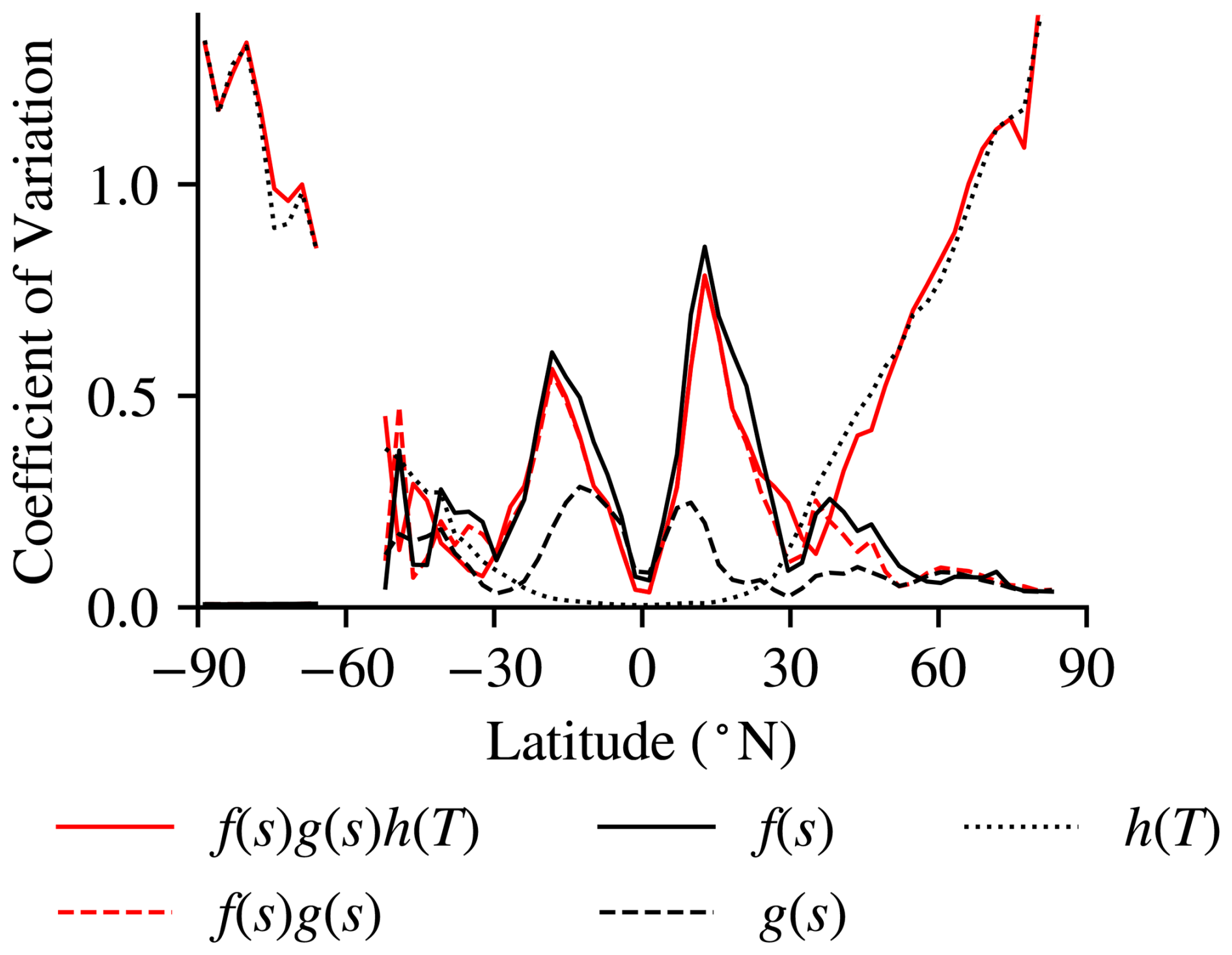
Figure 6 Coefficient of seasonal variation for the zonal-mean prototype deposition scheme (solid red); the factors that vary with soil moisture (dashed red); and terms f (solid), g (dashed), and h (dotted).

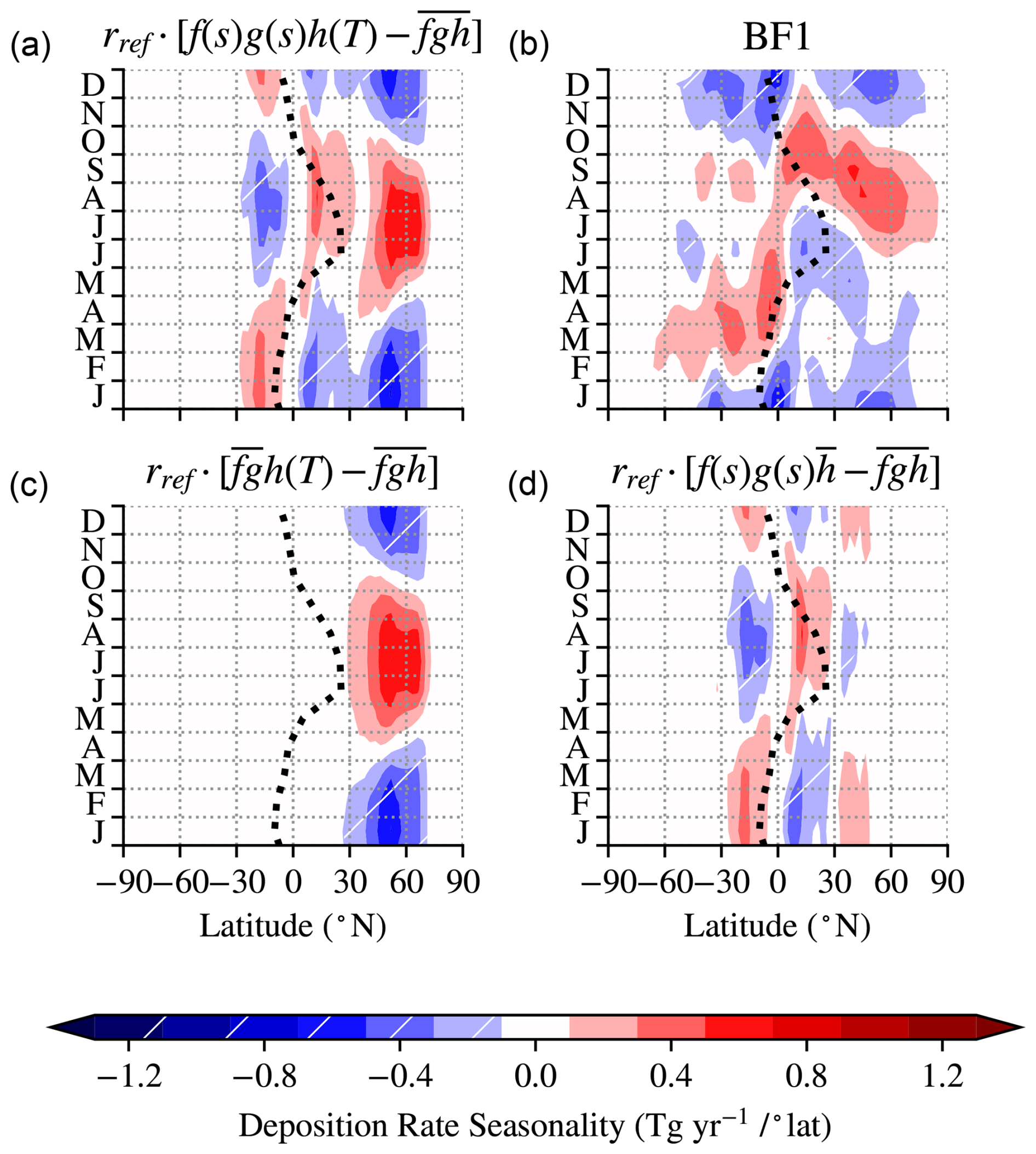
Figure 7 Deposition rate seasonality (shaded) for: (a) the prototype deposition scheme multiplied by the near-surface mixing ratios of this simulation; (b) BF1 from $\stackrel{\mathrm{‾}}{fgh}$ found in the inverted model;  (c) and (d) the prototype deposition scheme with isolated monthly variation that depends only on h and fg, respectively (Eq. 8). In each panel the ITCZ migration (black dots) is included as the order 10 precipitation centroid (from ERA5 2010–2020) between 20^∘S and 20° N following Adam et al. (2016).

An anomaly to the net surface flux is constructed as a perturbation to the prototype emissions and a perturbation to the prototype deposition scheme. We first identify the latitude–time signal of a deposition scheme that captures the best fit to the seasonality of the observations, independent of the seasonality of the prototype deposition scheme. This is the best-fit anomaly, BF1 (Table 2), required to reproduce r_ref from a model with a basic deposition state taken as the annual mean deposition velocity of the prototype scheme, $\stackrel{\mathrm{‾}}{fgh}$. BF1 is calculated as the average rate of relaxation of a number of small Newtonian relaxations, R, towards r_ref through each month of integration. This is found in an inverted version of the model, where the H₂ mixing ratio in the lower layer, r, changes as

$$\begin{array}{}\text{(9)}& {\displaystyle \frac{\partial }{\partial t}}r=S+M-r\stackrel{\mathrm{‾}}{fgh}-R,\end{array}$$

where

$$\begin{array}{}\text{(10)}& S=E+P-\text{rD}\end{array}$$

represents emissions, E, and atmospheric chemistry production, P, and destruction, rD, M represents mixing, and the relaxation term

$$\begin{array}{}\text{(11)}& R={\mathit{\delta }}_R(r-r_{\text{ref}}),\end{array}$$

where δ_R≪1 is a constant, is chosen such that r relaxes sufficiently close to r_ref by the end of the month but allows steady adjustment and mixing of r over that period. Note that, in this experiment, in the lower layer, the seasonality in r is much smaller than the annual mean such that $|r-r_{\text{ref}}|\ll \stackrel{\mathrm{‾}}{r}$, and ∼ 70 % of the total H₂ sink is by deposition into the soil (Sand et al., 2023) such that $\text{rD}\ll r\stackrel{\mathrm{‾}}{fgh}$. The net chemistry is assumed to be captured with the same monthly varying flux in each test.

We compare BF1 (Fig. 7b) with the seasonality of the prototype deposition scheme and its decomposed terms (Figs. 7a, c, and d). The seasonality of the prototype scheme, (fgh)^′, reproduces some key features of BF1. In particular, the prototype scheme captures the strong seasonality of BF1 in the NH mid-latitudes. There, seasonality is driven by the sensitivity of microbial activity to variation in soil temperature, which has been identified in laboratory microbial studies (Smith-Downey et al., 2006). Alternatively, the seasonality driven by soil moisture changes is dominant in the tropics.

To analyse how adjustments to the seasonality of the prototype deposition scheme affect results, we define R_BF(α,Δt) as the ratio of the RMS error between the seasonality of a deposition scheme – adjusted by scaling the seasonality of the prototype scheme by a factor α and offsetting in time by Δt – and BF1 to the RMS seasonality of BF1 at each latitude (Eq. D1). This ratio indicates how well the adjusted deposition scheme performs at reproducing the best-fit deposition scheme: R_BF=0 occurs where the adjusted scheme locally reproduces the best-fit scheme; R_BF=1 occurs if the adjusted scheme performs as well as the annual mean prototype deposition scheme, $\stackrel{\mathrm{‾}}{fgh}$; and R_BF>1 indicates that the adjusted scheme performs worse than $\stackrel{\mathrm{‾}}{fgh}$.

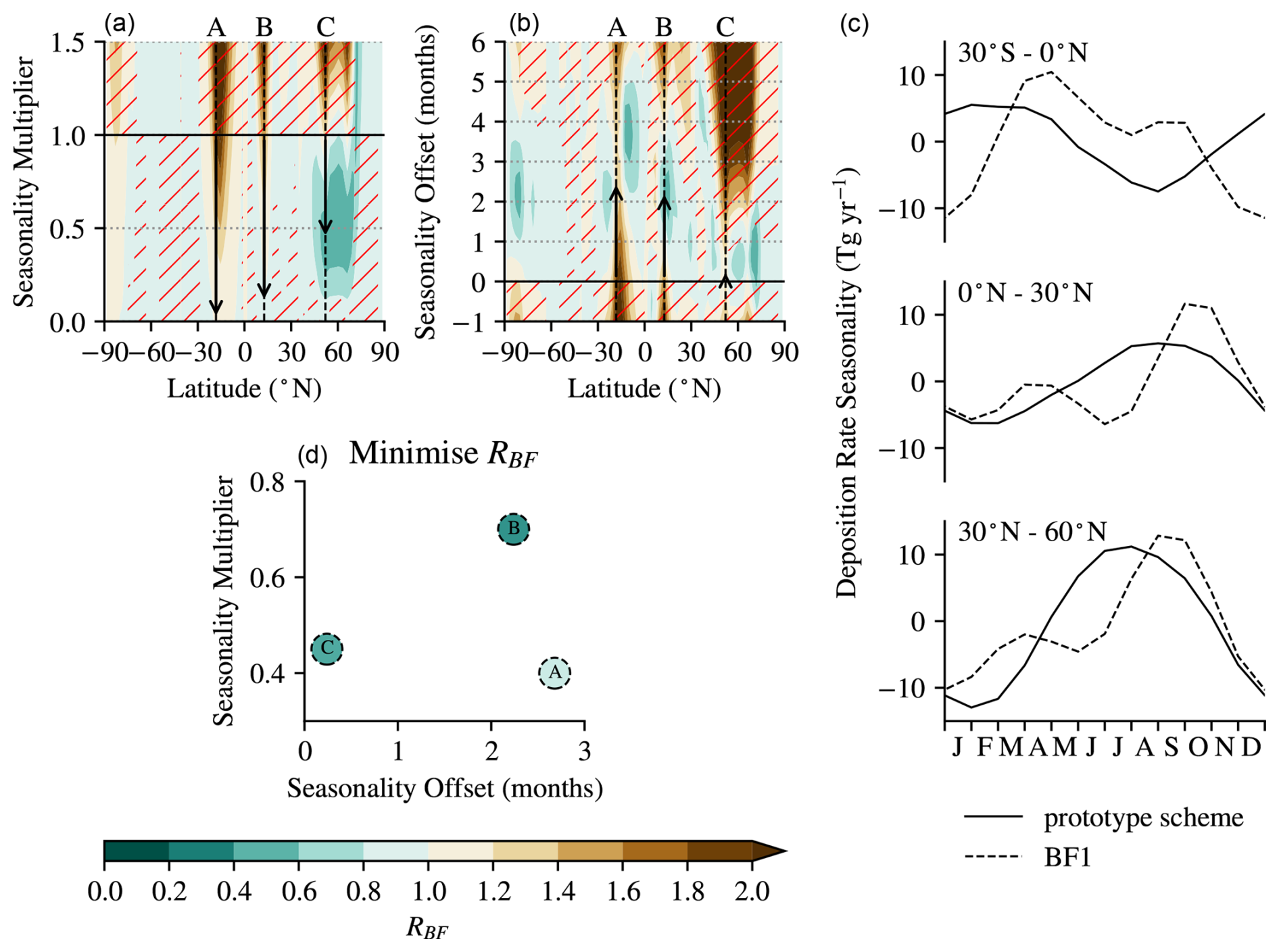
Figure 8 (a–c) Colours show R_BF (Eq. D1), which measures the performance of adjusted versions of the prototype deposition scheme at reproducing the best-fit deposition scheme, BF1. R_BF=1 when the adjusted scheme performs as well as the annual mean deposition with no seasonality, and R_BF=0 when the deposition scheme reproduces BF1. In (a), only the amplitude of the deposition seasonality is adjusted, by scaling with a multiplier, α. In (b), only the timing of the deposition seasonality is adjusted, by including an offset, Δt. Arrows indicate optimal adjustments at the latitudes of peaks in deposition seasonality in the prototype scheme (annotated A: 18° S, B: 13° N, and C: 52° N in each panel, see Fig. 7a) when α and Δt are adjusted individually. (c) The optimal R_BF achieved at latitudes A–C when α and Δt are adjusted jointly. Seasonality of deposition for the prototype and BF1 schemes, integrated across three latitude bands: (d) 0–30° S; (e) 0–30° N; and (f) 30–60° N.

In Fig. 8a, the seasonality of fgh only substantially reproduces BF1 where the strength of its seasonality is decreased in the temperate NH between 45 and 70° N. Alternatively, in Fig. 8b, fgh better reproduces the BF1 scheme when it includes a lag of 2 to 4 months in the tropics or half a month later in the NH mid-latitudes.

In Fig. 8c, the latitudes of peak amplitude of seasonality in the prototype scheme are isolated for optimised agreement with BF1 under adjustments to the seasonality multiplier and offset. In both deep tropical peaks (A, B), better agreement occurs for a lag of 2 to 3 months. Additionally, the strongest agreement occurs for weaker seasonality in the SH tropical peak (A). In the NH mid-latitudes, better agreement is achieved with a 1-week lag in the peak deposition at 52° N (C).

Figure 8c shows that R_BF is minimised when the amplitude of the seasonality decreases at A–C. However, this arises because BF1 is unconstrained by the seasonality in the prototype scheme, instead assuming that variations in deposition are spread across latitudes. By integrating the deposition seasonality across wider latitude bands, Fig. 8d and e show a lag and an increase in amplitude of seasonality between 30° S and 30° N, whereas Fig. 8f shows differences in the seasonal signal in the NH mid-latitudes but with a similar amplitude (cf. Figs.7a and b). The double peak in the deposition seasonality of BF1 in the tropics (Fig. 8d and e) suggests that the fastest uptake may occur coincidentally when the Intertropical Convergence Zone (ITCZ) crosses the Equator at the equinoxes (Fig. 8) rather than when the ITCZ is furthest from the Equator, as in the prototype scheme. This implies that BF1 may reflect a soil-moisture interaction that is not captured in the prototype scheme. Paulot et al. (2024) have recently shown how a deposition scheme driven by three-hourly varying soil parameters from the Global Land Data Assimilation System (Rodell et al., 2004) and a low soil moisture activation threshold for bacterial uptake produced a double peak in H₂ in the tropics and captured NH H₂ seasonality. This was distinct from their base simulation driven by monthly mean soil moisture where NH subtropical H₂ peaked 3 months earlier than observations, comparable with the prototype scheme driven by monthly mean ERA5 data in this work (Fig. 4b).

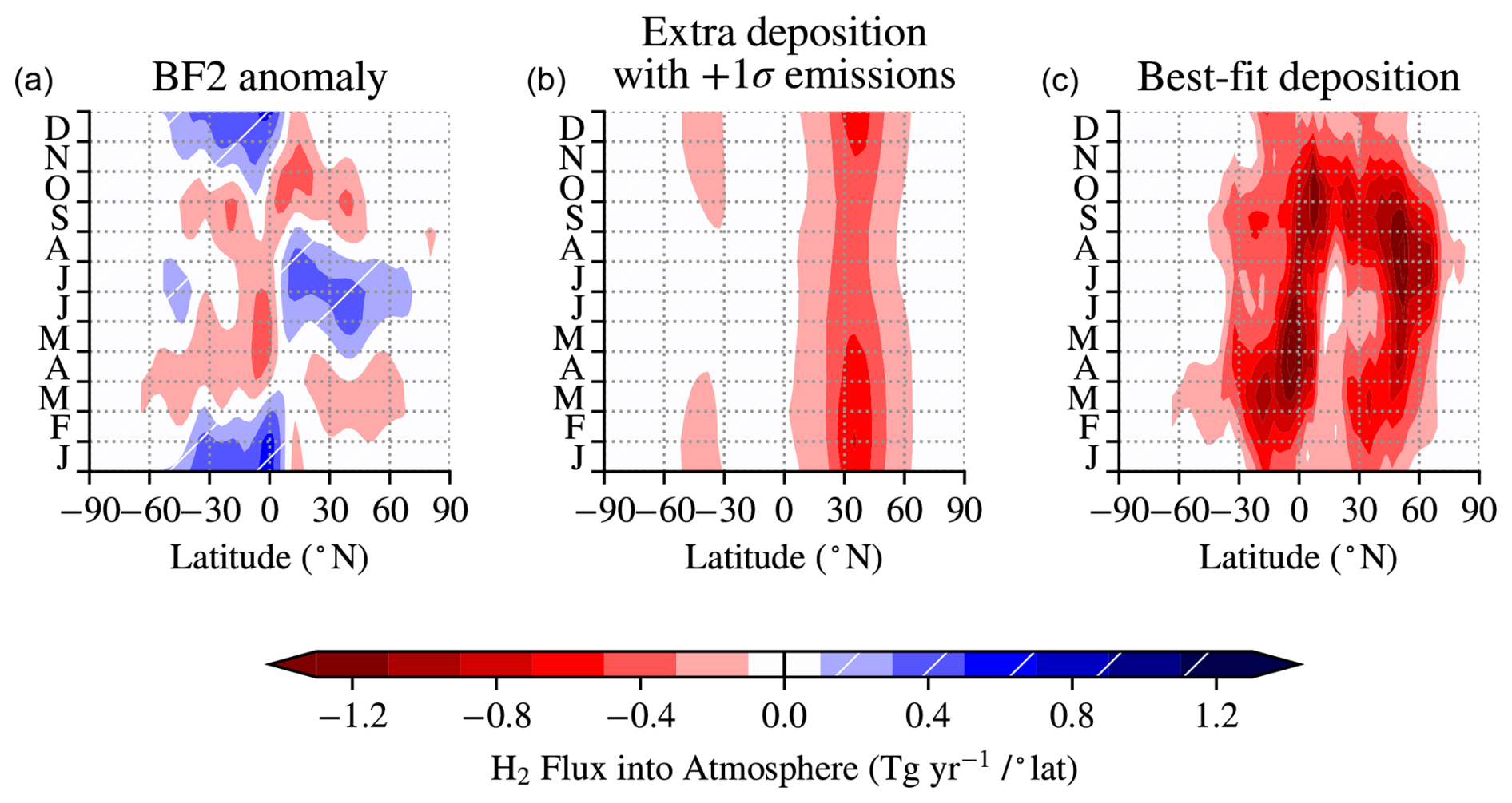
Figure 9 Different H₂ fluxes into the model: (a) BF2 anomaly into the lower layer to reproduce observations versus a simulation using the prototype deposition scheme; (b) anomaly change per +1σ change in “other emissions”; and (c) “best-fit deposition” under the prototype deposition scheme perturbed by BF2.

6 Contribution from emissions and chemical production and destruction

We have shown that the seasonality of the monthly varying prototype deposition scheme, fgh, captures the key features of a scheme that represents a best fit for the observed seasonality independent of the seasonality of the prototype scheme, BF1. Given that similar seasonal signals to the biophysics-based seasonality of the prototype scheme are independently reproduced by BF1, we examine a second best-fit scheme, BF2 (Table 2), derived as a perturbation from the full monthly varying prototype scheme. In this case, Eq. (9) becomes

$$\begin{array}{}\text{(12)}& {\displaystyle \frac{\partial }{\partial t}}r=S+M-rfgh-R,\end{array}$$

where S is unchanged but the mixing, M, and relaxation, R, terms respond to the change $\stackrel{\mathrm{‾}}{fgh}\to fgh$. Like BF1, BF2 is calculated from the flux anomaly (Fig. 9a) contained in R and required to resolve r_ref.

Due to the large inter-model spread in estimated H₂ emissions (Table 3,  Sand et al., 2023), it is necessary to consider how much of the BF2 anomaly may be explained by the assumed emissions (Fig. 5a and b) and chemistry (Fig. 5c) schemes. The BF2 anomaly is strongest in the tropics and subtropics with a net upwards flux peaking south of the Equator in November–December and spreading into the northern tropics during the NH summer. This upwards flux is similar to the source from biomass burning (Fig. 5a) displaced several months later, where other studies have used stronger emissions for biomass burning than the inputs4MIPS (Marle et al., 2017) scheme (e.g. Novelli, 1999; Sanderson et al., 2003; Price et al., 2007; Xiao et al., 2007). However, it also captures a weakening of the high deposition in the prototype deposition scheme driven by increases in f following the migration of the ITCZ (Fig. 7d). Combined with the stronger deposition during the winter in the subtropics of both hemispheres, this structure captures an offset in the prototype deposition scheme of around 3 months, as seen earlier for BF1 (Fig. 8c).

Alternatively, the upwards flux component of this anomaly may partly be explained by an intensification of emissions due to nitrogen fixing or net production by chemical processes during the summer in the subtropics and tropics. Increasing the intensity of non-biomass burning H₂ emissions by 1 standard deviation of the Sand et al. (2023) inter-model emissions estimate requires enhanced deposition, with a maximum of around 0.5 $\mathrm{Tg}{\mathrm{yr}}^{-\mathrm{1}}\mathrm{°}{\mathrm{lat}}^{-\mathrm{1}}$, focused in the NH mid-latitudes and peaking in both hemispheres between December and February (Fig. 9b).

7 Effect on H₂ lifetime of the perturbed scheme

To examine the effect of changing the prototype deposition scheme to the best-fit deposition scheme, BF2, we conduct a series of H₂ perturbation experiments. To gauge the sensitivity of changing the deposition scheme, timescales of deposition into the soil are calculated for 1-year integrations after the injection of small H₂ perturbations $r^{\prime }\ll r_{\text{ref}}$, noting that lifetimes will become more homogeneous for longer integrations as the remaining perturbation becomes more mixed into the atmosphere. For sufficiently small perturbations, we assume the chemistry fluxes are unchanged, and the anomalous flux is dominated by the soil flux (see Prather and Holmes, 2013). Likewise, we assume the differences between experiments with the prototype deposition scheme and BF2 are not obscured by using the same chemistry fluxes.

From the soil deposition timescales, an approximate total lifetime, τ_total, is calculated as the parallel addition of the lifetime due to chemical loss in the atmosphere, τ_atmchem = 7.7 years from Sand et al. (2023), and soil deposition timescales for each perturbation, with an approximate scaling factor $\mathrm{1000}/\mathrm{850}$ because the 2D model only extends to 150 hPa rather than the top of atmosphere, assuming that H₂ mixing ratios in the upper 150 hPa of the atmosphere are similar to those modelled between 1000 and 150 hPa (e.g. Warwick et al., 2004),

$$\begin{array}{}\text{(13)}& {\mathit{\tau }}_{\text{total}}^{-\mathrm{1}}\approx {\mathit{\tau }}_{\text{atmchem}}^{-\mathrm{1}}+{\left({\displaystyle \frac{\mathrm{1000}\mathrm{hPa}}{\mathrm{850}\mathrm{hPa}}}{\mathit{\tau }}_{\text{soil}}^{†,\ast }\right)}^{-\mathrm{1}},\end{array}$$

where ${\mathit{\tau }}_{\text{soil}}^{†,\ast }$ are model timescales calculated in different experiments.

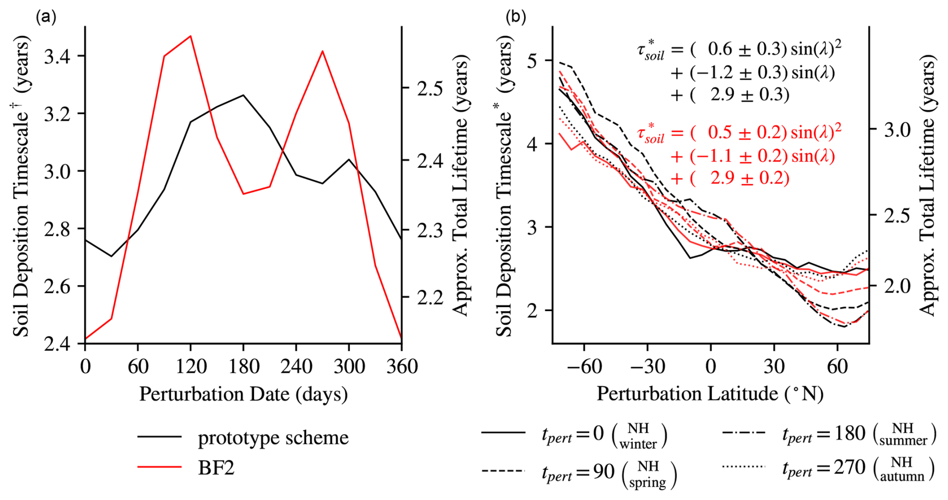
Figure 10 Soil timescales calculated from 1-year simulations with: (a) ${\mathit{\tau }}_{\text{soil}}^{†}$ calculated with whole troposphere 1 ppb perturbations initialised at a range of dates; and (b) ${\mathit{\tau }}_{\text{soil}}^{\ast }$ calculated with perturbations of 0.1 Tg in the lower 200 hPa in latitude bands – quadratic fits are made against sin latitude. In both cases, the soil lifetime is underestimated, as the atmosphere is only simulated through 1000–150 hPa and due to the relatively short simulation length; and in ^∗ near-surface perturbation configuration. Approximate τ_total is the harmonic sum of $\frac{\mathrm{1}}{\mathrm{0.85}}{\mathit{\tau }}_{\text{soil}}^{†,\ast }$ and τ_atmchem, which is assumed to have the constant value 7.7 years from Sand et al. (2023). Likewise, the 3.4-years soil deposition lifetime (from Sand et al., 2023) corresponds with 2.9 years in this scheme.

In two perturbation experiments, perturbations to H₂ are: † as +1 ppb throughout the simulated atmosphere initiated for each month (Fig. 10a); and ^∗ as +0.1 Tg in the lower 200 hPa layer through a continuum of latitude bands, initiated at 0, 90, 180, and 270 d to sample the sensitivity of the soil lifetime to the season of the emission (Fig. 10b). A soil lifetime is then calculated from the decay of each perturbation after 1 year.

In the prototype scheme, the SH deposition peaks at 10–20° S around 1 month into the year (Figs. 5d and 7b). In contrast, as shown in Fig. 9c, the best-fit SH deposition occurs in extended periods spreading northwards across the Equator from March to October and in the SH subtropics into the winter. In the NH mid-latitudes, BF2 has a similar temporal signal as the prototype scheme but with extensive deposition continuing into September.

In simulations using the prototype scheme, a whole-troposphere H₂ perturbation has the longest soil lifetime, τ_soil, when initialised around 150 d into the year – as a product of the seasonally high mixing ratio in the NH subtropics observed in Fig. 4b. τ_soil has a minimum for perturbations initialised around 30 d, when there is a high rate of deposition in the SH, but it is half a year out of phase with the peak deposition, which is concentrated in the NH (Fig. 7a).

Under BF2, τ_soil is decreased relative to the prototype scheme for perturbations injected around either solstice reflecting the stronger seasonality in both hemispheres (resolving Fig. 4a). This decreased lifetime is balanced by relatively longer soil lifetimes at the equinoxes, where perturbations mix and react in the atmosphere over a longer timescale before deposition.

There is a gradient of longer τ_soil for perturbations initialised near the surface in the SH to shorter τ_soil for those initialised in the NH (Fig. 10b), reflecting the greater soil sink in the NH. For perturbations initialised at low latitudes, the seasonality of τ_soil corresponds with that of whole-troposphere perturbations. However, this is inverted for perturbations initialised in the extratropical NH where τ_soil is longest for perturbations initialised in the autumn and winter. The longer soil deposition timescale in the SH corresponds with a result of Derwent (2023), who identified a monotonically decreasing GWP for H₂ emissions sources from the SH mid-latitudes to the NH mid-latitudes.

The same pattern is largely reproduced in simulations using BF2 but with a weaker meridional gradient. Quadratic fits of the annual mean τ_soil against equal area intervals (sin of the perturbation latitude, λ) result in τ_soil = 2.9 ± 0.2 years at the Equator, with a similar first degree gradient of −1.1 ± 0.1 years with BF2 compared to −1.2 ± 0.3 years with the prototype scheme, and an insignificant change in this negative gradient with latitude reflecting that BF2 only aims to resolve the seasonality in the observed H₂ distribution. However, there are distinct changes in seasonal lifetimes under BF2. In particular, SH extratropical perturbations are deposited more quickly when injected at 0 d, and NH extratropical perturbations are more slowly deposited when injected at 90 d.

8 Conclusions

The methods we have discussed provide a toolbox to constrain the development of H₂ deposition schemes using empirical observations of the zonal mean H₂ distribution and seasonality. In particular, we have identified the asymmetry in the seasonal cycle of H₂ in the NH and SH. Without a seasonally varying soil uptake, the seasonality of zonal mean surface H₂ would be dominated by the seasonality of atmospheric H₂ production and oxidation. H₂ concentrations would peak with similar amplitude during the late summer to early autumn in both the NH and SH extratropical regions (Fig. 4); the seasonality of the deposition induces a stronger amplitude and earlier peak in the NH H₂ signal.

We have shown that a prototype deposition scheme based on the assumed leading physical–biological processes of soil H₂ + uptake (Fig. 5d) effectively captures some key features of the planetary H₂ distribution in the 2D model. Assuming the annual mean of this prototype scheme as a suitable basic deposition state, we then produced a “best-fit” deposition scheme that reproduces the planetary H₂ seasonality independent of the seasonality of the prototype scheme. Comparing the seasonality of the best-fit scheme against the prototype scheme tested the accuracy of the seasonality of the prototype scheme. This challenges the assumed deposition seasonality in the tropics and provides useful insight into where similar deposition schemes should be revised to improve accuracy in future H₂ modelling efforts.

In the NH extratropics, the prototype scheme performs well in reproducing the observed annual mean meridional gradient and seasonality of surface H₂ mixing ratios. Simulations in the toolbox model produce H₂ mixing ratios in the SH that are too high, where Paulot et al. (2024) have reduced SH net ocean emissions in the extratropics compared with the emissions used in this study. However, we show how differences in phase and too weak an amplitude of seasonality in the southern tropics and subtropics may be resolved by the choice of the deposition scheme. We find that while the prototype scheme agrees with key features of the best-fit deposition scheme, the prototype deposition scheme would better reproduce observations with a lag of +2 to +3 months in its seasonality in the tropics. Other sources of hysteresis on the seasonality may be explained by dependence on irreversible degeneration of free enzymes in soils where seasonal temperatures fluctuate above 30 °C (Chowdhury and Conrad, 2010); variations in soil organic carbon content (King et al., 2008; Karbin et al., 2024); or even the life cycle of soil microbes (Meredith et al., 2014). Our results indicate that deeper investigations into the H₂ flux in tropical soils are needed to build our understanding of the links between these soil microbial processes and the planetary-scale H₂ signal.

A second best-fit deposition scheme was found by perturbing the monthly varying prototype scheme (Fig. 9c). In both the prototype and best-fit deposition schemes, there is strong seasonal and meridional dependence of the soil deposition timescale for different configurations of H₂ perturbations. The choice of the deposition scheme also had an impact on the meridional dependence of the soil lifetime for H₂ emissions injected at particular times of year.

When calculating the climate benefit of future hydrogen energy systems, such as by Hauglustaine et al. (2022), constraining the H₂ flux to soils may have a significant impact on the sensitive question of how accurately comprehensive models predict the spatial dependence of environmental impacts of H₂ emissions from regional industrial hydrogen projects (e.g. Derwent, 2023). This is particularly important in the SH, where soil deposition timescales are shorter for emissions during the summer in simulations with the best-fit scheme compared with the prototype scheme.

Appendix A

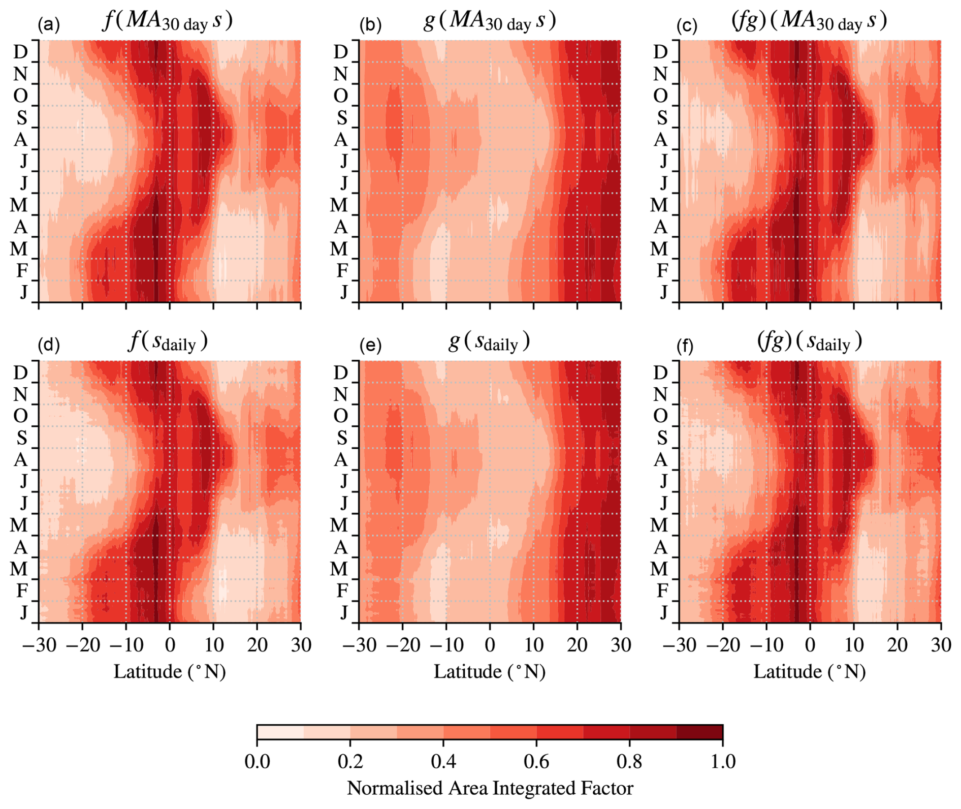
Figure A1 Comparison of soil moisture-dependent factors in the prototype deposition scheme under different temporal resolution ERA5 2010–2020 data in 30° S–30° N. (a) and (d) compare f; (b) and (e) compare g; and (c) and (f) compare the product fg. (a–c) are calculated with 30 d moving average soil moisture, MA_30 ds; and (d–f) are calculated with daily average soil moisture. The data are averaged for day in year excluding leap days. Area-integrated factors are normalised with the same multiplier in: (a) and (d); (b) and (e); and (c) and (f).

Appendix B

Anomalous sites are determined based on the RMS error of the sum of the first and second harmonics, h₁+h₂, versus the mid-filtered station time series, F_mid(data);

$$\begin{array}{}\text{(B1)}& \text{anomalous: }\sqrt{\sum _t(h_{\mathrm{1}}+h_{\mathrm{2}}-F_{\text{mid}}(\text{data}){)}^{\mathrm{2}}}>\mathrm{20}\mathrm{ppb}.\end{array}$$

This criterion identifies five station time series where the decomposition method could not fit harmonics (illustrated in Fig. 3).

Appendix C

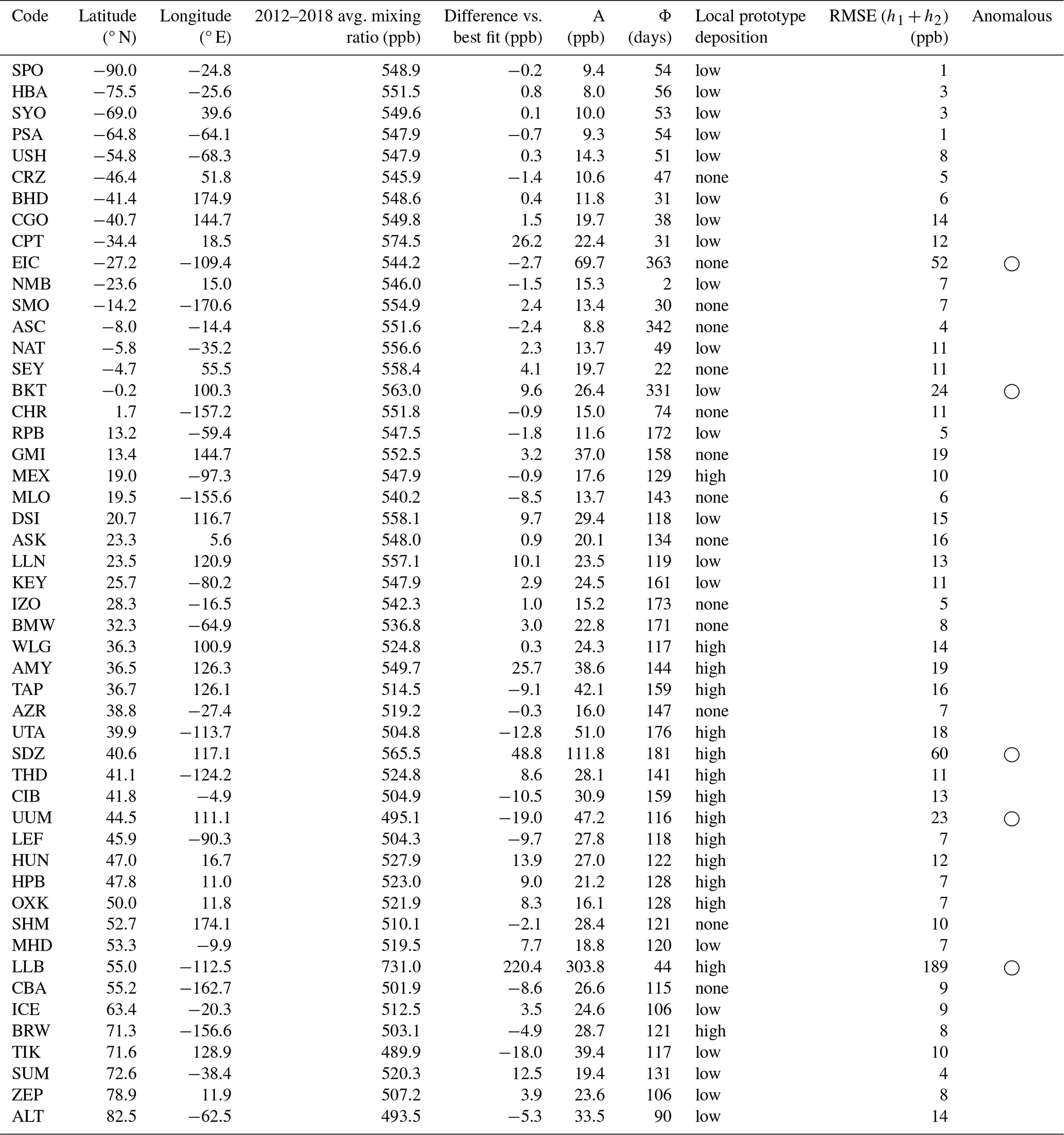
Table C1 Station data plotted in Figs. 2 and 4 with codes from Pétron et al. (2023) and difference versus best-fit average mixing ratio. Local prototype deposition is the average deposition within ± 2.5° N and ± 2.5° E: no deposition; low deposition $\in (\mathrm{0},\mathrm{0.2}]$ $\mathrm{g}{\mathrm{m}}^{-\mathrm{2}}{\mathrm{yr}}^{-\mathrm{1}}$; and high deposition >0.2 $\mathrm{g}{\mathrm{m}}^{-\mathrm{2}}{\mathrm{yr}}^{-\mathrm{1}}$. RMSE(h₁+h₂) is the RMS error of the fit versus the data (Eq. B1).

Appendix D

To analyse how adjustments to the seasonality of the prototype deposition scheme affect results, we define the ratio of the RMS error between the seasonality of an adjusted deposition scheme and BF1 to the RMS seasonality of BF1 at each latitude:

$$\begin{array}{}\text{(D1)}& R_{\text{BF}}(\mathit{\alpha },\mathrm{\Delta }t)={\displaystyle \frac{\sqrt{{\int }_t^{t+\mathrm{1}\text{year}}{\left(r_{\text{ref}}^{-\mathrm{1}}\text{BF1}-\mathit{\alpha }{W}^{\prime }(t^{\prime }-\mathrm{\Delta }t)\right)}^{\mathrm{2}}\mathrm{d}{t}^{\prime }}}{\sqrt{{\int }_t^{t+\mathrm{1}\text{year}}{\left(r_{\text{ref}}^{-\mathrm{1}}\text{BF1}\right)}^{\mathrm{2}}\mathrm{d}{t}^{\prime }}}},\end{array}$$

where the adjusted deposition seasonality $\mathit{\alpha }{W}^{\prime }(t-\mathrm{\Delta }t)$ is the seasonality of the prototype scheme, (fgh)^′, scaled by a factor α and offset in time by Δt.