Responses of polar energy budget to regional sea surface temperature changes in extra-polar regions

Surface temperature at polar regions not only is affected by local forcings and feedbacks but also depends on teleconnections between polar regions and low-latitude regions. In this study, the responses of the energy budget in polar regions to remote sea surface temperature (SST) changes are analyzed using a set of idealized regional SST perturbation experiments. The results show that the responses of the polar energy budget to remote sea surface warmings are regulated by changes in atmospheric energy transport, and radiative feedbacks also contribute to the polar energy budget at both the top of atmosphere (TOA) and the surface. Specifically, an increase in poleward atmospheric energy transport to polar regions results in an increase in surface and air temperature, and the corresponding Planck feedback leads to radiative warming at the surface and radiative cooling at the TOA. In response to sea surface warmings in most mid-latitude regions, poleward atmospheric energy transport to polar regions in the corresponding hemisphere increases. Sea surface warming over most tropical regions enhances the polar energy transport to both Arctic and Antarctic regions, except that an increase in the Indian Ocean's temperature results in a decrease in poleward atmospheric energy transport to the Arctic due to the different responses of stationary waves. The sensitivity of the Arctic energy budget to tropical SST changes is generally stronger than that of the Antarctic energy budget, and poleward atmospheric heat transport is dominated by dry static energy, with a lesser contribution from latent heat transport. The polar energy budget is not sensitive to SST changes in most subtropical regions. These results help to explain how the polar climate is affected by the magnitude and spatial pattern of remote SST change.

1 Introduction

As the global surface temperature increases, the Arctic region has experienced a surface temperature rise of more than twice the global average (Lenssen et al., 2019), a phenomenon known as “Arctic amplification” (AA). On the other hand, Antarctic warming is weaker compared to Arctic warming due to the higher average elevation of the Antarctic continent, lower albedo, feedback efficiency differences, and the Southern Ocean's heat absorption capacity (Marshall, 2003; Salzmann, 2017; Smith et al., 2019; Hahn et al., 2021). The polar energy budget is highly sensitive to various local feedback mechanisms. One important mechanism is the ice–albedo feedback. Global warming reduces snow cover and sea ice cover in the polar regions, leading to more solar radiation being absorbed, which in turn accelerates climate warming and further decreases albedo (Dickinson et al., 1987; Hall, 2004; Boeke and Taylor, 2018; Duan et al., 2019; Dai et al., 2019). Temperature feedback is another significant contributor to AA (Pithan and Mauritsen, 2014; Laîné et al., 2016; Sejas and Cai, 2016). It involves the processes of radiative cooling and is characterized by the Planck and lapse-rate feedbacks. The Planck feedback, driven by the nonlinear relationship between blackbody radiation and temperature, provides negative feedback to top of atmosphere (TOA) fluxes at all latitudes, especially in low latitudes (Pierrehumbert, 2010). The lapse-rate feedback is a significant driver of AA: in the Arctic regions, stable stratification and temperature inversions trap surface warming and reduce radiative cooling, thereby enhancing warming. In contrast, the tropics experience significant upper-atmosphere warming due to convection, which does not similarly trap heat (Pithan and Mauritsen, 2014). During climate warming, the transformation of ice clouds into water clouds increases cloud albedo, leading to negative feedback (Mitchell et al., 1989; Li and Le Treut, 1992). Simultaneously, the decrease in lower-tropospheric stability increases Arctic cloud cover and optical thickness (Barton et al., 2012; Solomon et al., 2014; Taylor et al., 2015; Yu et al., 2019), contributing to Arctic autumn and winter warming (Boeke and Taylor, 2018). These local feedbacks are considered the primary contributors to AA (Pithan and Mauritsen, 2014; Goosse et al., 2018; Hahn et al., 2021; Dai et al., 2019).

The polar climate is also affected by remote influences, whose interaction drives Arctic warming (Li et al., 2021). While some studies suggest that remote forcing plays a relatively minor role in AA (Stuecker et al., 2018), other research highlights the significant impact of poleward heat and moisture transport from lower latitudes in enhancing Arctic warming, and AA exists even in the absence of local sea ice feedbacks (Alexeev et al., 2005; Graversen and Burtu, 2016). Specifically, poleward atmospheric heat transport (AHT) and moisture transport are critical components that contribute substantially to the observed warming in the Arctic.

Under global warming, the AHT from low latitudes is more effective in reaching the polar regions compared to the equatorward transfer from high latitudes (Alexeev et al., 2005; Chung and Räisänen, 2011; Park et al., 2018; Shaw and Tan, 2018; Semmler et al., 2020), and multiple global climate model experiments have been conducted to measure the remote influence on Arctic warming (Alexeev et al., 2005; Chung and Räisänen, 2011; Yoshimori et al., 2017; Park et al., 2018; Shaw and Tan, 2018; Stuecker et al., 2018; Semmler et al., 2020). The transport of water vapor from mid-latitudes also plays an important role by enhancing the greenhouse effect prior to condensation and increasing cloudiness after condensation, which together warm the Arctic during winter (Graversen and Burtu, 2016). Graversen and Burtu (2016) showed that latent heat transport can lead to significantly more Arctic warming than dry static energy (DSE) transport, even when delivering an equivalent amount of energy. Therefore, remote processes play an important role in driving Arctic warming, and the remote forcings are further amplified by local feedback processes.

In low-latitude regions, sea surface temperature (SST) variations markedly affect the polar energy budget (Alexeev et al., 2005). It is widely accepted that planetary waves play a critical role in establishing teleconnections between tropical oceans and polar regions. These waves are pivotal in the transport of heat and moisture to the Arctic, consequently driving the increase in polar temperatures (Graversen and Burtu, 2016; Baggett and Lee, 2017). For instance, intensified convective activity within the Pacific Warm Pool not only strengthens the propagation of Rossby waves toward the poles but also increases the frequency of these fluctuations. This enhancement in Rossby wave activity boosts the transport of water vapor to the Arctic, augmenting the downward longwave radiation in the Arctic regions (Rodgers, 2003; Lee et al., 2011; Lee, 2012, 2014). While synoptic-scale transient eddies contribute significantly to mean-state poleward heat transport and its changes under increased CO₂ (Donohoe et al., 2020), their overall impact is relatively minor compared to that of amplified planetary waves in response to tropical warming (Baggett and Lee, 2017). Atmospheric circulation models reveal that the warming of tropical SST from glacial to interglacial periods significantly elevates summer temperatures in regions where the Canadian ice sheet (also known as the Laurentide ice sheet) forms. Conversely, cold tropical SST perturbations exert a lesser impact on water vapor transport and temperature in the Canadian region (Rodgers, 2003). The tropical SST anomalies during El Niño and La Niña events have a large impact on Arctic surface air temperature (Lee et al., 2011; Lee, 2012, 2014), but the impacts of major El Niño events on Arctic temperatures are distinct due to differences in eastern tropical Pacific SST (Jeong et al., 2022), indicating that the amplitude and spatial pattern of SST change are important for Arctic climate predictions.

In previous research, scholars primarily focused on the impact of SST on the polar energy budget over a large area of tropical oceans. However, studies have indicated significant variations in the effects of SST anomalies on the global climate system in different oceanic regions (Barsugli and Sardeshmukh, 2002; Fletcher and Kushner, 2011). In this study, we employ a set of idealized SST patch experiments to perform a systematic analysis of the response of the polar energy budget to SST changes in various areas.

2 Data and method

2.1 Individual patch experiments

The patch experiments were conducted using the Community Earth System Model version 1.2.1 integrated with the Community Atmospheric Model version 5.3 (CESM1.2.1-CAM5.3; Neale et al., 2012), operating at a spatial resolution of 1.9° latitude by 2.5° longitude. The experimental setup included a control experiment and two sets of patch experiments – one with warm patches and another with cold patches. The control experiment spanned 41 years, maintaining the SST, sea ice, and climatic forcings at the constant present-day levels observed (in the year 2000). The global ocean was segmented into 80 overlapping rectangular areas, comprehensively covering the global ice-free ocean surface, as depicted in Fig. 1 of Zhou et al. (2020). In the warm patch experiments, a positive SST anomaly was introduced at the ocean surface within a designated patch, while the SST in other regions was the same as the control setup. Conversely, the cold patch experiments involved introducing a negative SST anomaly at the ocean surface within the respective patches. The SST anomalies in each patch were designed according to the equation proposed by Barsugli and Sardeshmukh (2002), which effectively mitigates nonlinearity due to unrealistic SST gradients, ensuring a more realistic simulation of oceanic temperature variations:

$$\begin{array}{}\text{(1)}& \begin{array}{rl}\mathrm{\Delta }{\text{SST}}_P& (\text{lat},\text{long})=\\ & A{\cos }^{\mathrm{2}}\left({\displaystyle \frac{\mathit{\pi }}{\mathrm{2}}}{\displaystyle \frac{\text{lat}-{\text{lat}}_{\mathrm{p}}}{{\text{lat}}_{\mathrm{w}}}}\right)\left({\displaystyle \frac{\mathit{\pi }}{\mathrm{2}}}{\displaystyle \frac{\text{long}-{\text{long}}_{\mathrm{p}}}{{\text{long}}_{\mathrm{w}}}}\right),\end{array}\end{array}$$

where $|\text{lat}-{\text{lat}}_{\mathrm{p}}|<{\text{lat}}_{\mathrm{w}}$, $|\text{long}-{\text{long}}_{\mathrm{p}}|<{\text{long}}_{\mathrm{w}}$. The terms lat_p and long_p are the latitude and longitude of the center point for a specific patch, respectively; lat_w and long_w are the meridional and zonal half-width of the patch, respectively, with their values set to lat_w=10° and long_w=40° in these experiments; and A is the amplitude of the SST anomaly, which is set to be +4 and −4 K in this study.

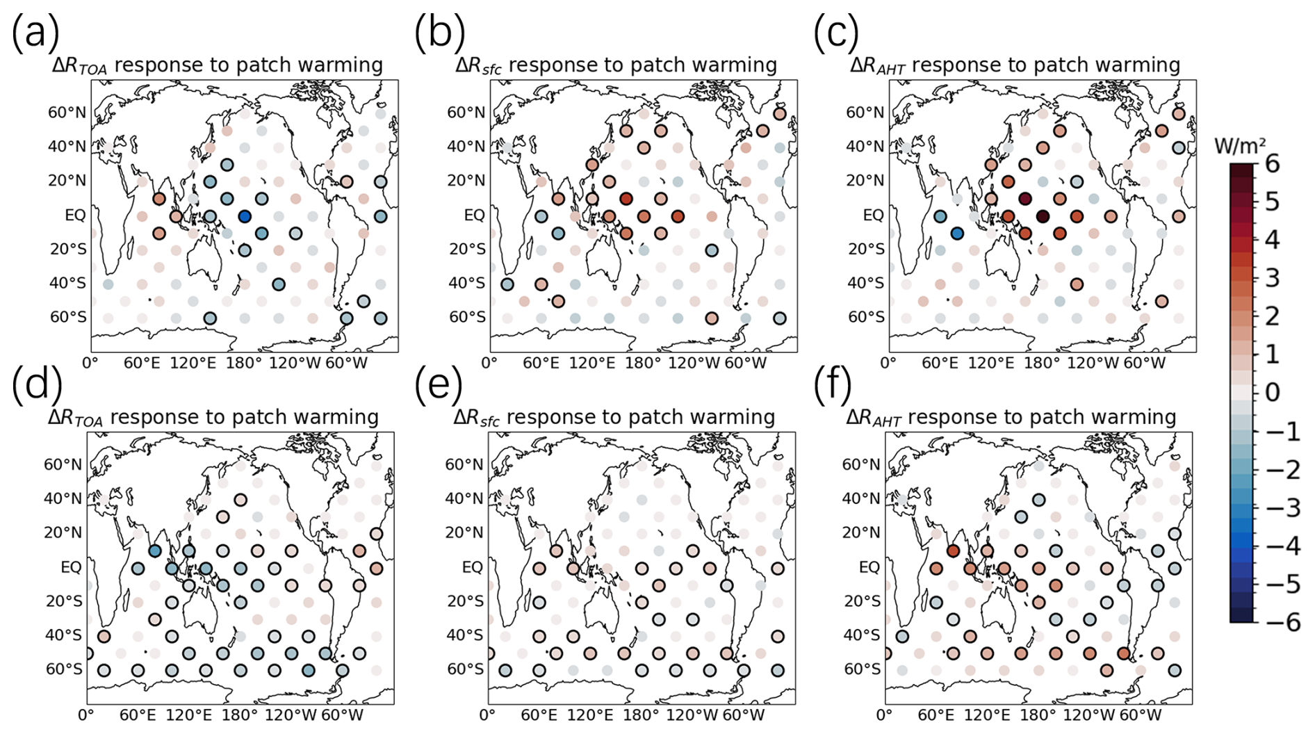
Figure 1 Responses of the polar energy budget to regional SST changes. (a) Differences in Arctic (60–90° N) annual mean net TOA radiative fluxes (ΔR_TOA) between conjugate warming and cooling patch experiments. (b) Differences in Arctic annual mean net surface radiative fluxes (ΔR_sfc). (c) Differences in heat fluxes due to the atmospheric heat transport to the Arctic regions (ΔR_AHT). (d, e, f) Responses of ΔR_TOA, ΔR_sfc, and ΔR_AHT in the Antarctic regions. The location of each point denotes the center of the corresponding patch, and the colors denote the differences between conjugate warming and cooling patch experiments. Black circles indicate that the differences are statistically significant at a 95 % confidence level.

In this study, we analyzed the responses of polar TOA radiative fluxes (R_TOA), polar surface fluxes (R_sfc), and heat fluxes resulting from atmospheric heat transport to the polar regions (R_AHT). The equations for calculating these parameters are listed as follows:

$$\begin{array}{}\text{(2)}& {\displaystyle }{R}_{\text{TOA}}=\text{FSNT}-\text{FLNT},\text{(3)}& {\displaystyle }{R}_{\text{sfc}}=\text{FSNS}-\text{FLNS}-\text{SH}-\text{LH},\text{(4)}& {\displaystyle }{R}_{\text{AHT}}=R_{\text{sfc}}-R_{\text{TOA}},\end{array}$$

where FSNT represents the net downward shortwave radiation at the TOA; FLNT denotes the net upward longwave radiation at the TOA; FSNS is the net downward shortwave radiation at the surface; FLNS represents the net upward longwave radiation at the surface; and SH and LH account for the sensible and latent heat fluxes, respectively. Additionally, both SH and LH are defined as positive upward.

2.2 EOF-SST experiments

To quantify the polar energy budget response to realistic SST anomaly patterns, we applied an empirical orthogonal function (EOF) analysis to historical SST data from 1980 to 2019, obtained from the Hadley Centre Sea Ice and Sea Surface Temperature dataset (HadISST; Rayner et al., 2003), and identified the first eight EOF modes. The first eight EOF modes explain approximately 55 % of the total variance in global SST anomalies, thereby representing the predominant variability patterns. We then conducted eight separate EOF-SST experiments, and the SST of each experiment was perturbed by a specific EOF mode relative to the control run. These experiments allow us to isolate and understand the impact of realistic SST anomaly patterns on the polar energy budget.

2.3 Radiative kernel decomposition methodology

This study employs the radiative kernel approach (Soden et al., 2008; Huang et al., 2017) to decompose both surface and TOA radiation into the radiative effects of various meteorological variables, measured in watts per square meter (W m⁻²). The core calculation involves multiplying the radiative kernels by the monthly anomalies of the corresponding climate fields as follows:

$$\begin{array}{}\text{(5)}& \mathrm{\Delta }{R}_X=K_X\cdot \mathrm{\Delta }X,\end{array}$$

where X denotes an arbitrary non-cloud climate variable; ΔR_X represents the radiative effect at the surface or TOA associated with that variable; K_X is the corresponding radiative kernel; and ΔX is the monthly anomaly of the climate variable, calculated as the deviation from the monthly climatological average. Positive values of ΔR indicate an increase in net incoming radiation, which corresponds to a warming effect on the Earth. The radiative kernels used in this analysis are derived from the ERA-Interim climatological fields and have been validated to perform well with the climate model surface outputs (Huang et al., 2017; Liu et al., 2024).

Cloud radiative effects are calculated following the methodology of Soden et al. (2008):

$$\begin{array}{}\text{(6)}& \mathrm{\Delta }{R}_{\text{cld}}=\mathrm{\Delta }\text{CRF}-{\sum }_X(K_X-K_X^{\mathrm{0}})\mathrm{\Delta }X.\end{array}$$

In this equation, ΔR_cld denotes the cloud-induced radiative anomalies, and CRF (cloud radiative forcing) is defined as the difference in surface net radiation fluxes between all-sky and clear-sky conditions. The superscript 0 means the clear-sky kernels.

Building upon this framework, the study further decomposes the TOA and surface radiative anomalies into specific feedback components to achieve a more detailed analysis of the factors influencing the Earth's radiation balance. ΔR_TOA is partitioned into cloud-induced radiative anomalies (ΔR_TOA,cld), albedo-induced radiative anomalies (ΔR_TOA,alb), Planck-feedback-induced radiative anomalies (ΔR_TOA,plk), and lapse-rate-feedback-induced radiative anomalies (ΔR_TOA,LR). Similarly, ΔR_sfc is broken down into cloud-induced surface radiative anomalies (ΔR_sfc,cld), albedo-related surface radiative anomalies (ΔR_sfc,alb), Planck-feedback-induced surface radiative anomalies (ΔR_sfc,plk), lapse-rate-feedback-induced surface radiative anomalies (ΔR_sfc,LR), LH anomalies (ΔLH), and SH anomalies (ΔSH).

3 Results

3.1 Responses of polar energy budget to local SST changes

The differences in the annual polar energy budget in conjugate SST warming patch experiments and SST cooling patch experiments are shown in Fig. 1. The location of each point denotes the center of the corresponding patch, and the colors of these points denote the differences in the polar energy budget between corresponding conjugate warming and cooling patch experiments. Additionally, t tests were conducted to assess their statistical significance. The difference between TOA radiation (Fig. 1a and d) and surface radiation (Fig. 1b and e) reflects atmospheric heat transport (Fig. 1c and f).

Figure 1a–c show the responses of the Arctic energy budgets to SST warmings in global oceanic regions. In response to western and central tropical Pacific SST warming, there is a significant increase in poleward energy transport toward the Arctic regions (Fig. 1c), as indicated by the positive poleward heat transport to the Arctic region (positive ΔR_AHT). This enhanced energy transport warms the Arctic atmosphere, leading to an increase in surface radiation (positive ΔR_sfc, Fig. 1b) due to higher surface and air temperatures. Simultaneously, the warmer atmosphere emits more longwave radiation into space, resulting in a decrease in TOA radiation (negative ΔR_TOA, Fig. 1a). Conversely, warming in the tropical Indian Ocean reduces the poleward energy transport to the Arctic region (negative ΔR_AHT), leading to cooler Arctic atmospheric temperatures, and there is a decrease in surface radiation (negative ΔR_sfc, Fig. 1b) and an increase in TOA radiation (positive ΔR_TOA, Fig. 1a). Sea surface warming in the mid-latitudes of the Northern Hemisphere increases Arctic surface radiation but has an insignificant impact on TOA radiation.

For the Antarctic energy budget, warming in the tropical Pacific and Indian oceans generally leads to increased poleward energy transport (positive ΔR_AHT, Fig. 1f), which warms the Antarctic atmosphere and results in increased Antarctic surface radiation (positive ΔR_sfc, Fig. 1e) and decreased Antarctic TOA radiation (negative ΔR_TOA, Fig. 1d). However, the response of ΔR_TOA to warmings in the tropical Atlantic is positive (Fig. 1d). Warming in the Southern Ocean also leads to an increase in Antarctic surface radiation and a decrease in Antarctic TOA radiation. The Antarctic energy budget is generally not sensitive to warmings in subtropical regions. Both ΔR_TOA and ΔR_sfc decrease in response to warmings in patches centered at 60° S, because patches centered at 60° S cover part of the Antarctic region (60 to 90° S in this study), and the surface emits more energy into space as the sea surface warms, leading to a cooling radiative effect.

The response of Arctic ΔR_AHT to tropical warmings is generally greater than Antarctic ΔR_AHT, indicating that more heat is transported to the Arctic region than to the Antarctic region when the tropics warm. This difference may partly contribute to faster Arctic warming than Antarctic warming under global warming.

The responses of the polar energy budget depend on the season. The spatial distribution of the Arctic polar energy budget response to regional SST in boreal winter (DJF) (Fig. 2a–c) is similar to the annual average values (Fig. 1a–c), but the magnitude of the DJF responses is greater than the annual responses. For the Antarctic region, the response of the DJF polar energy budget to tropical ocean warming aligns with the annual average values.

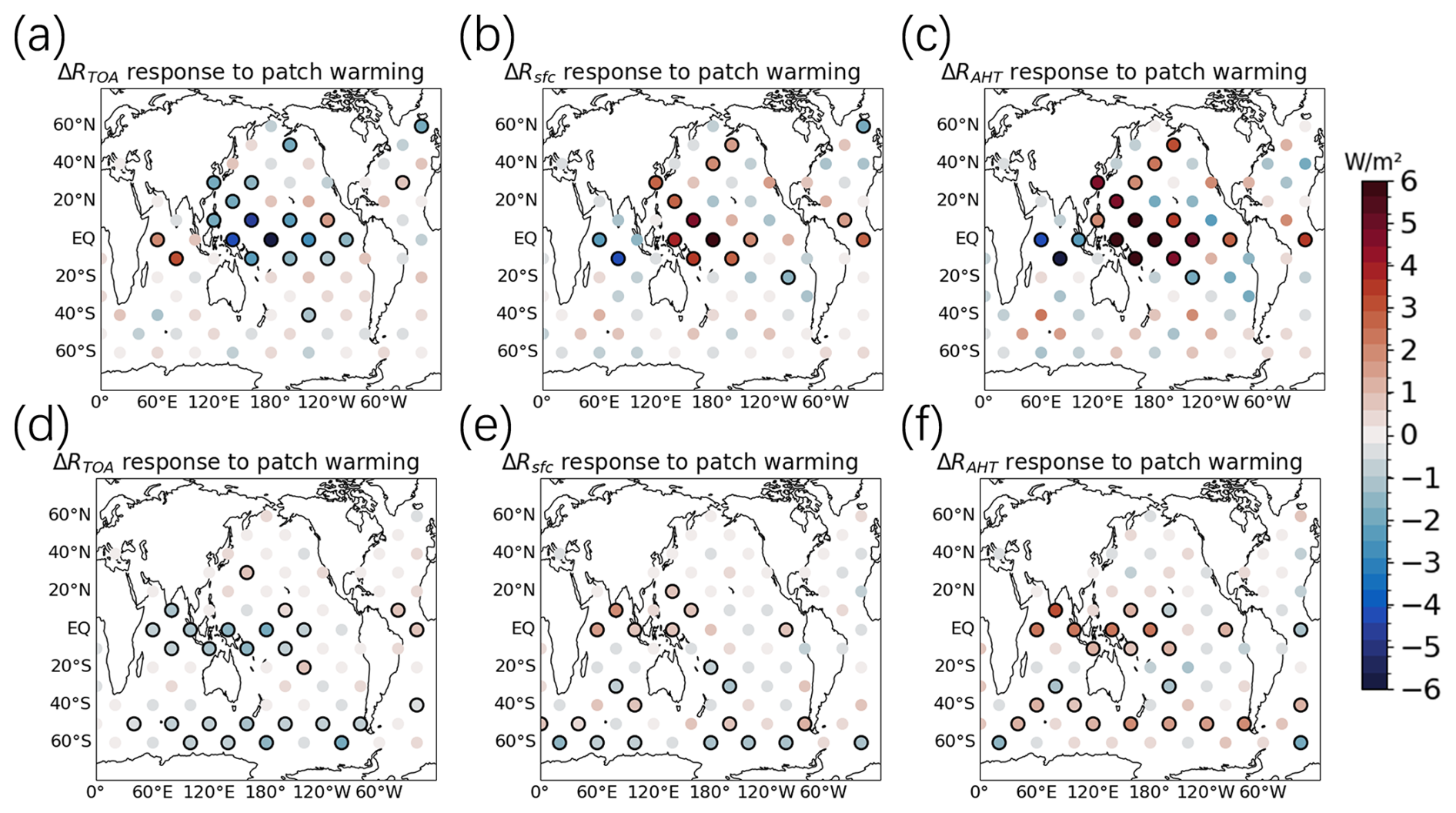
Figure 2 The same as Fig. 1, but for the DJF season.

During boreal summer (JJA), the spatial distribution of the Arctic polar energy budget responses (Fig. 3a–c) differs from the annual average. Specifically, the responses of ΔR_AHT to warmings in both the Indian Ocean and the western Pacific Ocean are positive. The responses of ΔR_sfc and ΔR_TOA in most patch experiments are statistically insignificant. Conversely, the Antarctic polar energy budget responses to tropical ocean warming in JJA are similar to the annual mean values.

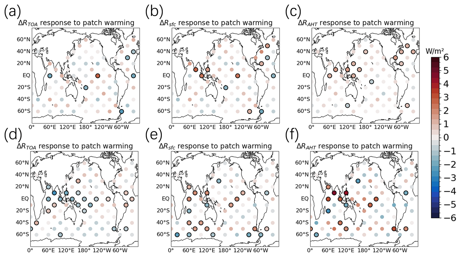
Figure 3 The same as Fig. 1, but for the JJA season.

3.2 Reconstruction using Green's function

The response of the polar energy budget to regional SST changes might be used to qualitatively explain how SST variations affect the polar energy budget.

The sensitivity of the polar energy budget to SST perturbations within a specific grid box, identified by index i, can be estimated using the following equation (Zhou et al., 2017):

$$\begin{array}{}\text{(7)}& {\displaystyle \frac{\partial R}{\partial {\text{SST}}_i}}={\displaystyle \frac{{\sum }_P\mathrm{\Delta }{\text{SST}}_P\frac{\partial R}{\partial {\text{SST}}_P}\frac{S_i}{S_P}}{{\sum }_P\mathrm{\Delta }{\text{SST}}_P}},\end{array}$$

where R denotes a specific energy flux; SST_i denotes the SST in the ith grid box; S_i and S_P represent the ocean surface area of the specific grid point and the patch, respectively; and ΔSST_P is the SST anomaly of the ith grid in the pth patch. $\frac{\partial R}{\partial {\text{SST}}_P}$ is the sensitivity of R to patch-averaged SST change, which is derived from experiments for the corresponding warming and cooling patch experiments. The sensitivity to grid boxes within a single patch corresponds to the average R change due to a 1 K warming within that specific grid box. The sensitivities of the polar energy budget to SST perturbation in each grid box are shown in Fig. 4.

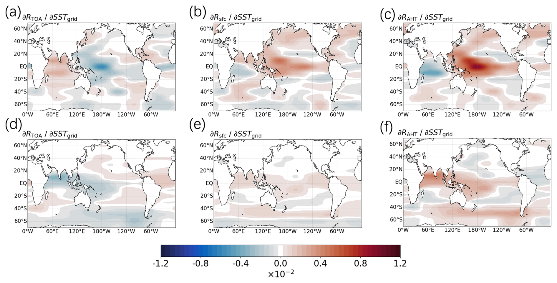
Figure 4 Sensitivity of (a) $\partial R_{\text{TOA}}/\partial {\text{SST}}_i$ of Arctic, (b) $\partial R_{\text{sfc}}/\partial {\text{SST}}_i$ of Arctic, (c) $\partial R_{\text{AHT}}/\partial {\text{SST}}_i$ of Arctic, (d) $\partial R_{\text{TOA}}/\partial {\text{SST}}_i$ of Antarctic, (e) $\partial R_{\text{sfc}}/\partial {\text{SST}}_i$ of Antarctic, and (f) $\partial R_{\text{AHT}}/\partial {\text{SST}}_i$ of Antarctic to surface warming in each grid box, calculated using Eq. (7). The units are $\mathrm{W}{\mathrm{m}}^{-\mathrm{2}}{\mathrm{K}}^{-\mathrm{1}}$.

Utilizing these sensitivities, we can reconstruct the polar energy budget response to arbitrary changes in SST through Green's function approach, represented as

$$\begin{array}{}\text{(8)}& \mathrm{\Delta }R={\mathrm{\Sigma }}_i{\displaystyle \frac{\partial R}{\partial {\text{SST}}_i}}\mathrm{\Delta }{\text{SST}}_i+{\mathit{\epsilon }}_{\mathrm{1}},\end{array}$$

where ε₁ is an error term which represents the contributions from nonlinearities and non-SST-induced factors.

Then we use Green's function approach to reconstruct the ΔR_AHT in response to eight different SST patterns in the EOF-SST experiments (Fig. 5a–h). ΔR_AHT reconstructed by Green's function is then compared to model-produced values in the EOF-SST experiments (Fig. 5i and j). The results show that the majority of the experimental simulations of ΔR_AHT align closely with the ΔR_AHT reconstructed by Green's function, lying near the y=x line. The biases of the values reconstructed by Green's function are partially induced by the SST change in the Arctic region, which is not captured by the Green's function reconstruction, and nonlinear terms also contribute to the bias. Therefore, Green's function approach can qualitatively explain how the SST perturbation patterns in Fig. 5a–h affect the polar energy budget.

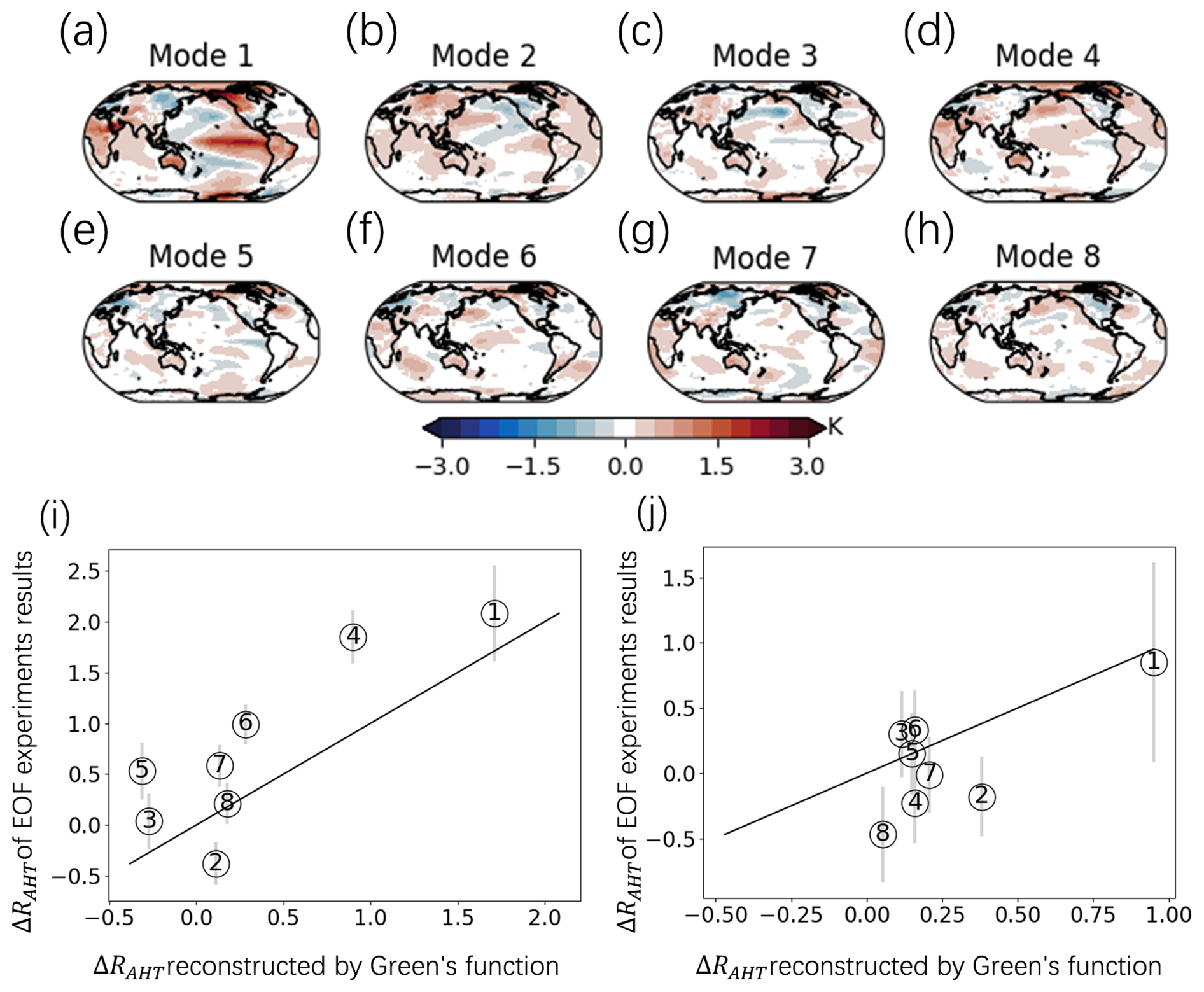
Figure 5 (a–h) Surface temperature change patterns in individual EOF-SST experiments. (i) Comparison of Arctic ΔR_AHT responses to different SST change patterns in EOF-SST experiments (y axis) and that reconstructed by Green's function approach (x axis). All values are averaged annually in this figure. The digits represent the number of corresponding EOF modes in each experiment. Error bars correspond to the 95 % confidence interval. (j) Response of Antarctic ΔR_AHT.

3.3 Decomposition of polar energy budget responses with radiative kernels

To understand the mechanism of how the polar energy budget is affected by remote SST, we quantify the contributions of meteorological factors to the polar energy budget responses (Figs. 6 and 7) using radiative kernels (Huang et al., 2017).

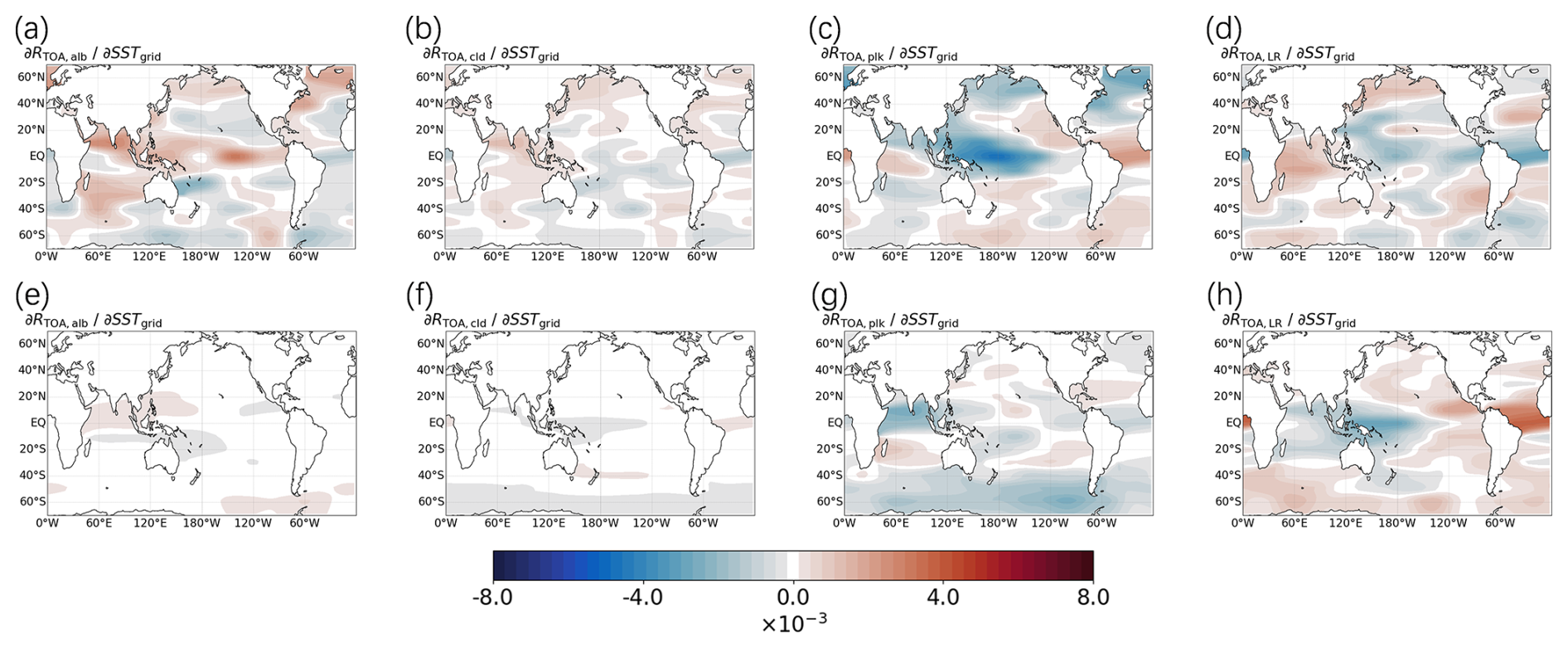
Figure 6 Sensitivity of annual mean ΔR_TOA,cld (a), ΔR_TOA,alb (b), ΔR_TOA,plk (c), ΔR_TOA,LR (d) for Arctic and annual mean ΔR_TOA,cld (e), ΔR_TOA,alb (f), ΔR_TOA,plk (g), and ΔR_TOA,LR (h) for Antarctica between conjugate warming and cooling patch experiments. The units are $\mathrm{W}{\mathrm{m}}^{-\mathrm{2}}{\mathrm{K}}^{-\mathrm{1}}$.

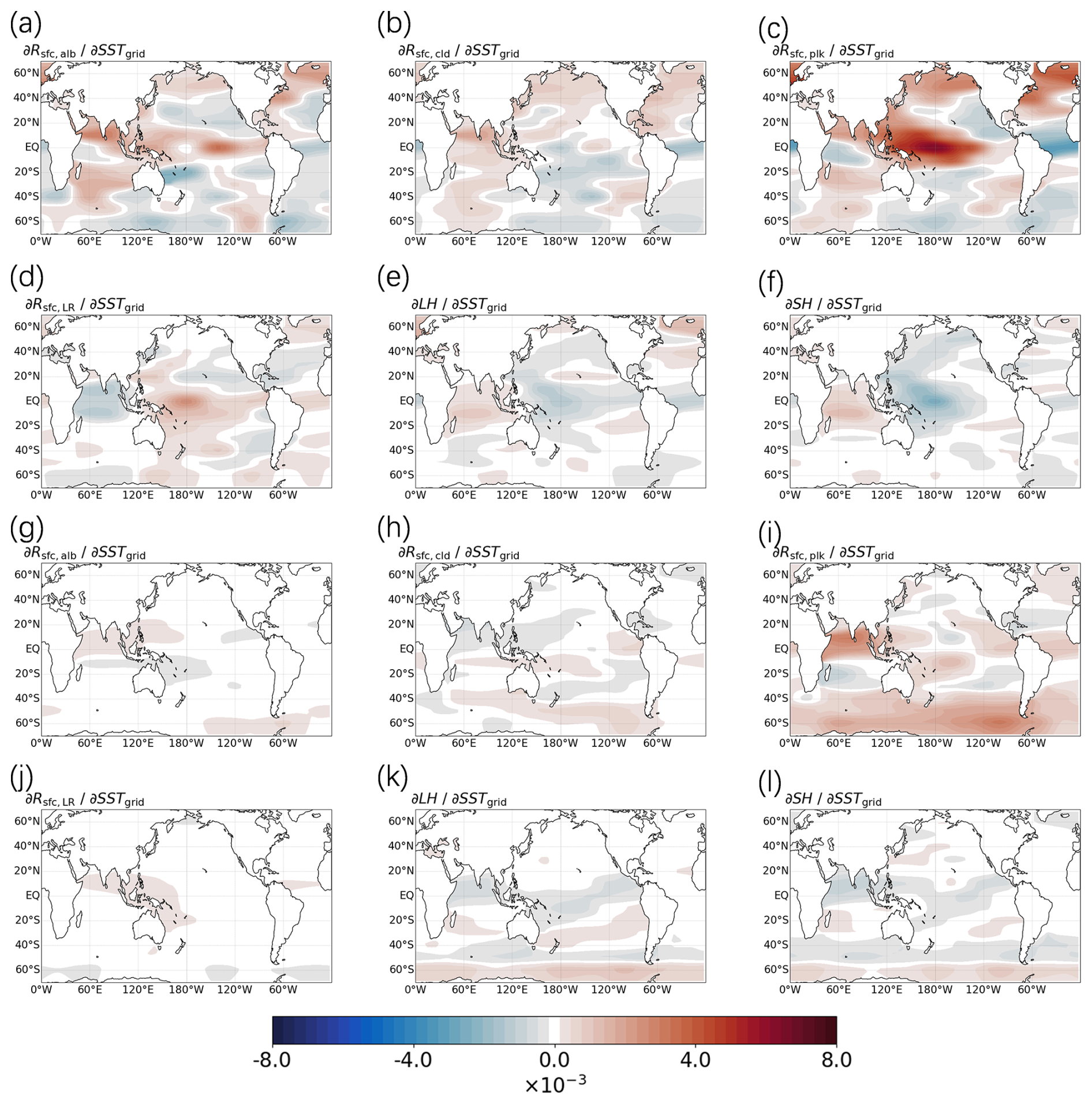
Figure 7 Sensitivity of annual mean ΔR_sfc,cld (a), ΔR_sfc,alb (b), ΔR_sfc,plk (c), ΔR_sfc,LR (g), ΔLH (h), ΔSH (i) for the Arctic region, and annual mean ΔR_sfc,cld (d), ΔR_sfc,alb (e), ΔR_sfc,plk (f), ΔR_sfc,LR (j), ΔLH (k), and ΔSH (l) for the Antarctic region between conjugate warming and cooling patch experiments. The units are $\mathrm{W}{\mathrm{m}}^{-\mathrm{2}}{\mathrm{K}}^{-\mathrm{1}}$.

Figure 6a shows that the contribution of cloud changes is relatively small compared to the Arctic ΔR_TOA response. Pacific SST warming results in a negative Arctic ΔR_TOA,cld, whereas Indian Ocean warming generates a positive Arctic ΔR_TOA,cld. Albedo exhibits a positive response in both the tropical Indian Ocean and the Pacific Ocean (Fig. 6a). The impact of Arctic ΔR_TOA,plk exhibits a positive response to SST increases in the tropical Indian Ocean and a negative response to the tropical western Pacific (Fig. 6c), indicating that the Planck feedback is the primary contributor to Arctic ΔR_TOA. The sensitivity of Arctic ΔR_TOA,LR to SST increases exhibits a negative response to warming in the tropical western Pacific, while showing a positive response in the Indian Ocean (Fig. 6d). The Planck feedback's response to SST warming is approximately twice that of the lapse-rate feedback.

For the Antarctic, the contribution of clouds to the ΔR_TOA response is minimal (Fig. 6f), as is the contribution of albedo changes to the Antarctic ΔR_TOA response (Fig. 6e). In contrast to the Arctic, the Antarctic ΔR_TOA response to SST changes is jointly dominated by Planck and lapse-rate feedbacks. Warming in the Indian Ocean induces a stronger negative ΔR_TOA,plk (Fig. 6g), whereas warming in the Pacific leads to a more pronounced negative ΔR_TOA,LR (Fig. 6h). Additionally, warming in the tropical Atlantic triggers a notably strong positive ΔR_TOA,LR (Fig. 6h).

Figure 7 shows the contributions of meteorological factors to the responses of Arctic and Antarctic ΔR_sfc. For the Arctic, the spatial distribution of clouds' contribution to Arctic ΔR_sfc is similar to that for Arctic ΔR_TOA, but the values are significantly higher (Fig. 7b). The response of Arctic ΔR_sfc,alb closely resembles that of ΔR_TOA,alb, with similar magnitudes (Fig. 7a). Similar to the response of Arctic ΔR_TOA,plk, the Arctic ΔR_sfc,plk response is also strong (Fig. 7c), but the signs of ΔR_sfc,plk responses are generally opposite to those of the ΔR_TOA,plk response. The response of Arctic ΔR_sfc,LR to tropical ocean warming also shows signs opposite to those of ΔR_TOA,LR (Fig. 7d). Over the tropical Indian Ocean, Planck feedback is positive in the northern region and negative in the southern region, whereas lapse-rate feedback is consistently negative across the entire tropical Indian Ocean. Overall, Planck feedback remains dominant for Arctic ΔR_sfc. The responses of Arctic ΔLH and Arctic ΔSH are negative in response to warmings in the tropical western Pacific and positive in response to warmings in the tropical Indian Ocean (Fig. 7e and f), although these factors have a minor impact on Arctic ΔR_sfc. The negative responses of Arctic ΔLH and Arctic ΔSH in response to warmings in the tropical western Pacific indicate a suppression of upward turbulent heat fluxes at the Arctic surface, primarily due to enhanced energy transport from lower latitudes into the Arctic region. As warm air masses are advected poleward, the associated increase in downward longwave radiation warms the Arctic surface. This warming stabilizes the lower atmospheric boundary layer, thereby reducing the vertical turbulence necessary for effective heat exchange between the surface and the atmosphere.

Similar to the Arctic regions, the contribution of clouds to Antarctic ΔR_sfc is small (Fig. 7h). Albedo has no significant impact on Antarctic ΔR_sfc (Fig. 7g), because sea ice concentration is fixed in these patch experiments, and snow cover in Antarctica does not change significantly in these experiments. The Planck feedback dominates the contributions to Antarctic ΔR_sfc, with Antarctic ΔR_sfc,plk responding positively to tropical ocean warming (Fig. 7i). Similar to the Arctic, the lapse-rate feedback contributes less significantly to ΔR_sfc (Fig. 7j). Antarctic ΔLH and Antarctic ΔSH show minimal responses, with opposite signs to ΔR_sfc,plk (Fig. 7k and l). These results suggest that while temperature adjustments are notable in Antarctica, the responses of cloud cover and surface heat fluxes to remote SST warming have a small impact on Antarctic ΔR_sfc.

3.4 AHT responses to regional SST changes

According to Figs. 6 and 7, the Planck feedback, which is primarily driven by changes in temperature, is the primary contributor to the polar energy budget responses in these experiments. The sign of ΔR_AHT is generally the same as ΔR_sfc,plk and the opposite of ΔR_TOA,plk. In addition, the difference between TOA and the surface energy budget reflects the contribution of changes in polar AHT. Therefore, AHT plays a critical role in determining the polar energy budget by changing the air temperature of polar regions. The responses of AHT to SST perturbations in the mid-latitudes are consistent with our intuition, but the opposite Arctic AHT responses to SST warming over the tropical Indian Ocean (TIO) and tropical Pacific Ocean (TPO) require further investigations.

To explore the underlying mechanisms of this phenomenon, we compare the climate responses to warmings in two illustrative patches within the TPO and TIO. The center of the illustrative TPO patch is 0° N, 180° E, and the center of the illustrative TIO is 0° N, 60° E.

Figure 8 presents the responses of surface temperature (ΔT_s), 200 hPa geopotential height (ΔZ₂₀₀), and 500 hPa geopotential height (ΔZ₅₀₀) to warmings in these patches, providing background information to later AHT studies. Consistent with previous studies (Annamalai et al., 2007; Barsugli and Sardeshmukh, 2002; Ding et al., 2014), our experiments reveal that SST anomalies in different ocean basins induce contrasting atmospheric circulation patterns, primarily through Rossby wave responses affecting the Pacific–North American (PNA) pattern.

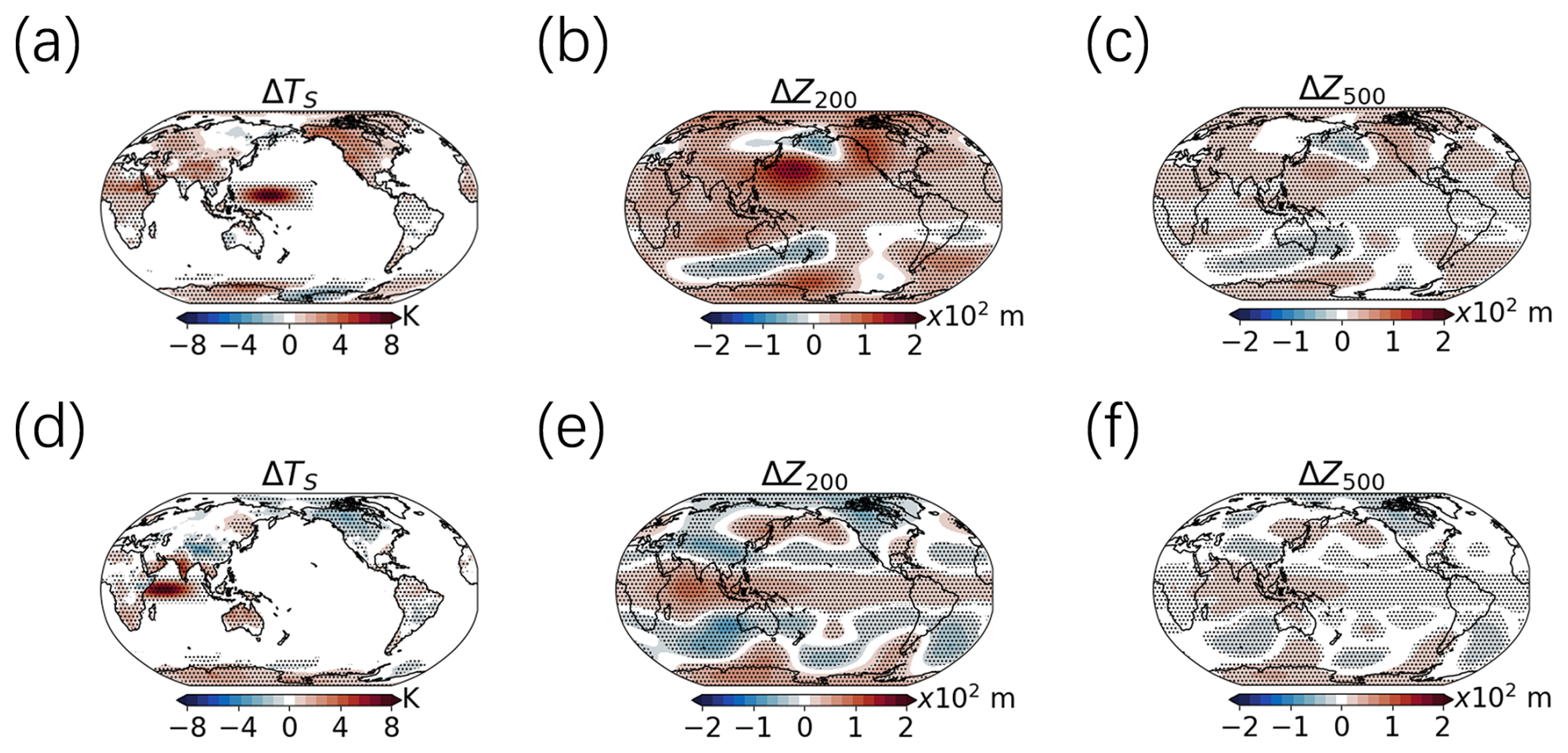
Figure 8 Spatial distributions of responses in ΔT_s (a), ΔZ₂₀₀ (b), and ΔZ₅₀₀ (c) following increased SST in a patch over the tropical Pacific Ocean (TPO) and in ΔT_s (d), ΔZ₂₀₀ (e), and ΔZ₅₀₀ (f) following increased SST in a patch over the tropical Indian Ocean (TIO). Dotted areas indicate regions that passed the 95 % confidence test.

Specifically, warming in the TPO region leads to an increase in ΔT_s over the Tibetan Plateau, eastern Europe, tropical Africa, northeastern North America, and most of the Antarctic regions. Concurrently, ΔZ₂₀₀ exhibits a local increase over the TPO region, a decrease over the North Pacific, and an increase over northeastern North America and Antarctic regions. The ΔZ₅₀₀ response mirrors the ΔZ₂₀₀ pattern but with reduced intensity. In contrast, warming in the TIO region induces ΔT_s increases over Antarctic regions and significant warming over the Indian subcontinent, while the Tibetan Plateau experiences cooling. Notably, the northwest of North America shows marked cooling under TIO warming. The ΔZ₂₀₀ response to TIO warming displays a dipole pattern, characterized by increases in the tropical warming regions and decreases toward the poles, followed by subsequent increases. The ΔZ₅₀₀ response follows a similar trend to ΔZ₂₀₀, with weaker intensity.

To quantify the impacts of SST warming over the TPO and TIO on the Arctic AHT, we computed the AHT responses to the warming of the two patches separately. AHT can be calculated as the vertically integrated and zonally averaged transport of moist static energy (S). According to Neelin and Held (1987), S can be defined as follows:

$$\begin{array}{}\text{(9)}& S=c_p{T}_{\mathrm{a}}+LQ+gZ,\end{array}$$

where T_a represents atmospheric temperature, c_p is the specific heat capacity of air at constant pressure, L denotes the latent heat of vaporization of water, Q is specific humidity, g is the acceleration due to gravity, and Z represents geopotential height. The components of S will be denoted below as S_T, S_Q, and S_Z, respectively.

The poleward transport of moist static energy S can be decomposed into mean meridional circulation (MOC), stationary eddy (SE), transient eddy (TE), and transient overturning circulation (TOC) components, following the methodologies of Priestley (1948) and Lorenz (1955). According to Donohoe et al. (2020), for each latitude θ, atmospheric energy transport is

$$\begin{array}{}\text{(10)}& \begin{array}{rl}& \mathrm{\text{AHT}}\left(\mathit{\theta }\right)=\\ & \mathrm{2}\mathit{\pi }\text{acos}\left(\mathit{\theta }\right){\int }_{\mathrm{0}}^{P_{\mathrm{s}}}\left[\stackrel{\mathrm{‾}}{V}\right]\left[\stackrel{\mathrm{‾}}{S}\right]+\stackrel{\mathrm{‾}}{\left[V^{\ast }{S}^{\ast }\right]}+\left[\stackrel{\mathrm{‾}}{V^{\prime \ast }{S}^{\prime \ast }}\right]+\stackrel{\mathrm{‾}}{\left[V{]}^{\prime }\right[S{]}^{\prime }}{\displaystyle \frac{\mathrm{d}p}{g}},\end{array}\end{array}$$

where V represents the meridional velocity. Square brackets ([  ]) denote zonal averages, overbars denote time averages over each month of analysis, asterisks (^∗) are departures from the zonal average, and primes (^′) are departures from the time average. The first term signifies the MOC driven by the vertical gradient in S, taking into account mass conservation in MOC energy transport. The second term is SE, showing poleward transport in warm or moist sectors. These first two terms can be calculated from monthly mean data. The third term pertains to the transport associated with TE, primarily baroclinic synoptic eddies. The fourth term involves energy transport by the covariance between zonal-mean overturning circulation and vertical stratification, referred to as TOC, which is significantly smaller than the other components and thus is often excluded in AHT discussions.

Figure 9 shows the changes in AHT and its components in response to warmings in the TPO and TIO. AHT response to warmings in the TPO at 60° N is positive, and AHT response to warmings in the TIO at 60° N is negative. For both cases, AHT to the Arctic region is dominated by SE (Fig. 9b), and the opposite SE response to the TPO and TIO leads to opposite responses in AHT, which also causes different responses of TOA and surface energy budgets in the Arctic regions. Additionally, Fig. 9c and d further dissect the SE responses to warmings in the TPO and TIO, respectively. The results indicate that dry static energy predominantly drives the SE response to warmings in both the TPO and the TIO.

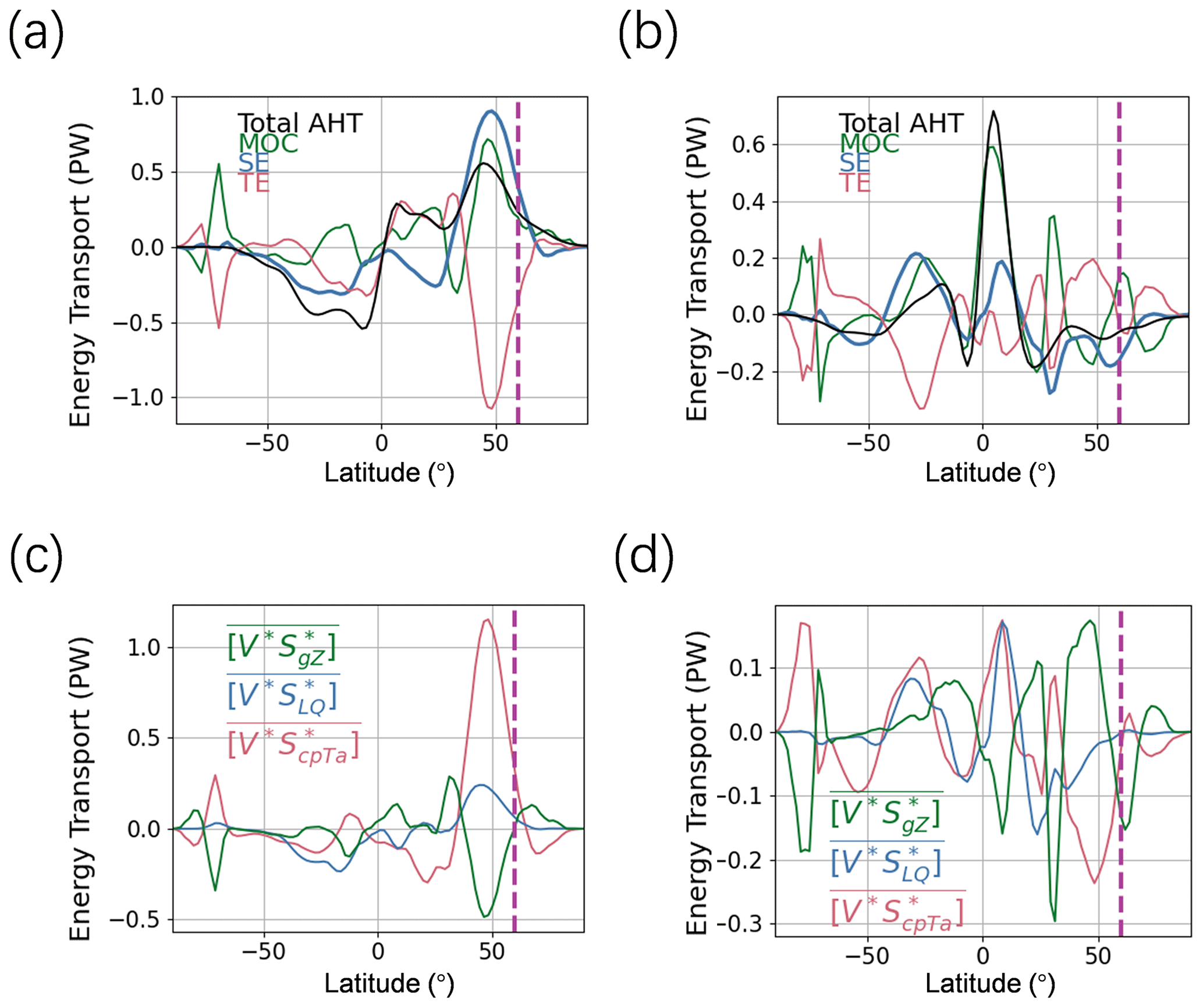
Figure 9 Decomposition of meridional AHT responses. Panels (a) and (b) show the changes in meridional AHT following SST warming in the TPO and TIO, respectively. The total AHT is represented by a thick black line, while the contributions from the MOC, SE, and TE are depicted by fine lines in green, blue, and red, respectively. Panels (c) and (d) detail the decomposition of the SE component from (a) and (b), with the contributions from Z, Q, and T shown in green, blue, and red, respectively. The dotted purple line represents the 60° N latitude line.

To better understand the opposite response of SE heat flux to warmings in the TPO and TIO, we analyzed the spatial distribution of SE heat fluxes. The vertically integrated SE heat flux (ϕ) can be computed through the following integral:

$$\begin{array}{}\text{(11)}& \mathit{\varphi }={\int }_{\mathrm{0}}^{P_{\mathrm{s}}}{V}^{\ast }{S}^{\ast }{\displaystyle \frac{\mathrm{d}p}{g}}.\end{array}$$

In response to warmings in the TPO, the vertically integrated SE heat flux exhibits significant oscillatory characteristics over the Pacific Ocean. According to Fig. 10a, ϕ increases in the tropical western and northwestern Pacific, decreases over the central Pacific, and then increases again over the northeastern Pacific and Alaska. Over land, ϕ increases over northeastern Asia, the Tibetan Plateau, and Europe. This phenomenon is consistent with Goss et al. (2016), who found that warming in the low-latitude Pacific leads to increased ϕ in higher latitudes.

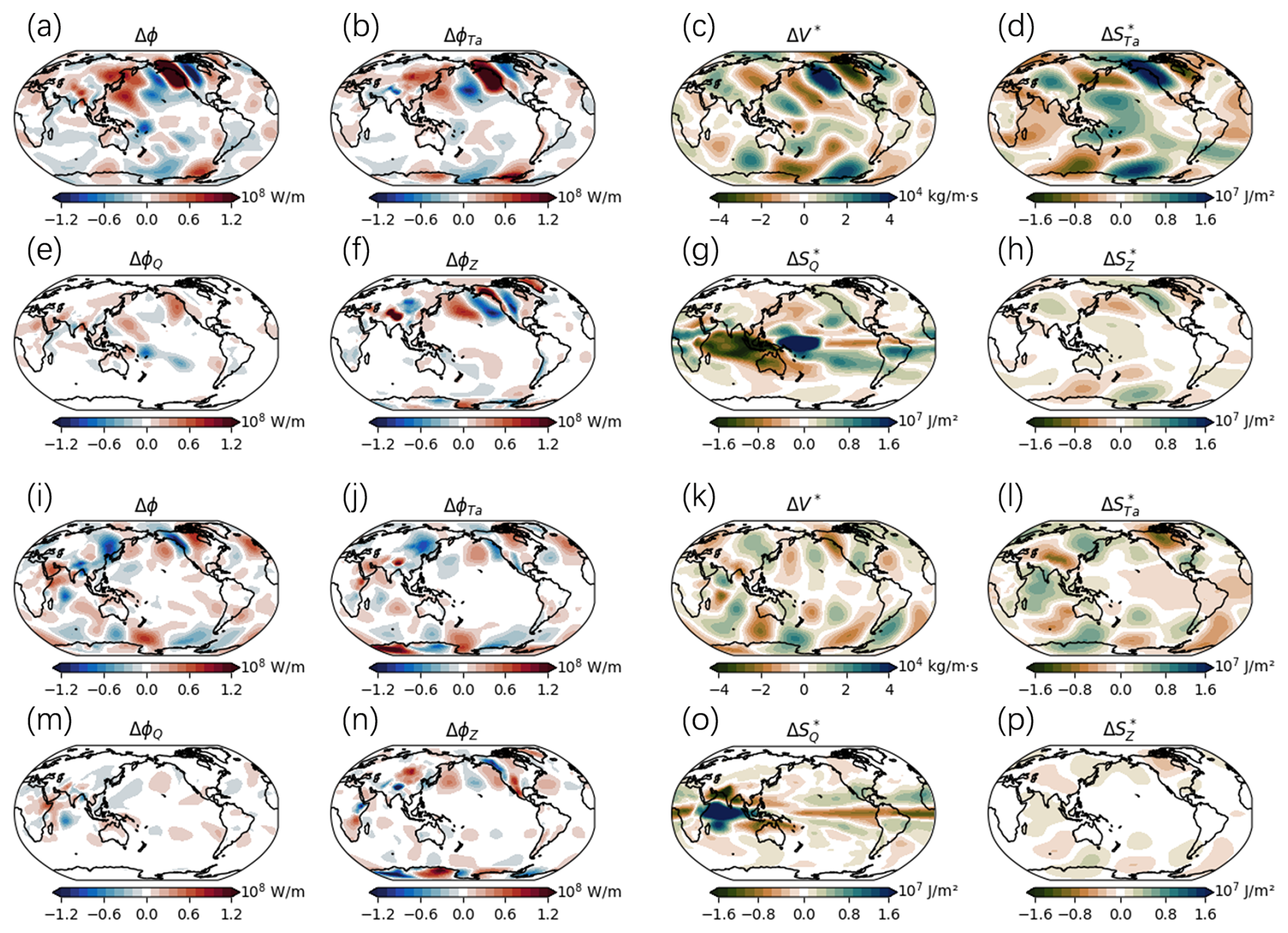
Figure 10 (a) Δϕ induced by SST warming in the TPO. (b) The contribution of Δϕ_Ta to the SE. (c) The vertical integration of ΔV^∗ from the surface to the TOA. (d) The vertical integration of $\mathrm{\Delta }{S}_{\text{Ta}}^{\ast }$ from the surface to the TOA. (e) The contribution of Δϕ_Q to the SE. (f) The contribution of Δϕ_Z to the SE. (g) The vertical integration of $\mathrm{\Delta }{S}_Q^{\ast }$ from the surface to the TOA. (h) The vertical integration of $\mathrm{\Delta }{S}_Z^{\ast }$ from the surface to the TOA. (i)–(p) are the same as (a)–(h) but for responses to warming in the TIO.

Combining Eqs. (9) and (11), we are able to further attribute ϕ to changes in dry static heat flux (Δϕ_Ta), latent heat flux (Δϕ_Q), and potential energy (Δϕ_Z), respectively. Among the three main contributing factors to Δϕ, Δϕ_Ta aligns closely with the overall Δϕ pattern, indicating it as the primary contributor (Fig. 10b). The spatial pattern of Δϕ_Ta can be explained by the change in ΔV^∗ and $\mathrm{\Delta }{S}_{\text{Ta}}^{\ast }$ (Fig. 10c and d), which reflects the spatial pattern of stationary waves. In addition, Δϕ_Q is large in the low latitudes but is small near the poles (Fig. 10e). Interestingly, Δϕ_Z exhibits an opposite pattern to Δϕ in the Northern Hemisphere (Fig. 10f). Despite the changes in $\mathrm{\Delta }{S}_Z^{\ast }$ that have a similar spatial distribution to $\mathrm{\Delta }{S}_{\text{Ta}}^{\ast }$ (Fig. 10h), Δϕ_Z shows an opposite trend to Δϕ_Ta due to the differing correlation between ΔV^∗ and $\mathrm{\Delta }{S}_Z^{\ast }$. This indicates that while $\mathrm{\Delta }{S}_Z^{\ast }$ increases in regions where ΔV^∗ also increases, their combined effect on Δϕ_Z leads to a negative contribution compared to Δϕ.

In response to warmings in the TIO, the spatial pattern of Δϕ oscillation is quite different from the TPO case. The transfer of SE heat flux encounters obstacles near the Tibetan Plateau, which might explain why the response of Δϕ is different in the Northern Hemisphere and the Southern Hemisphere. Globally, Δϕ_Ta remains the dominant contributor to Δϕ, while Δϕ_Q's contribution remains relatively low. Notably, in the Tibetan Plateau region, Δϕ_Z becomes the primary driver of Δϕ (Fig. 10i and n).

Based on these results, we are able to understand why the responses of AHT near 60° N to warmings in the TPO and TIO are different. The response of stationary waves to warmings in these two regions is different, so the poleward moist static energy transported by SE is also different, leading to opposite AHT responses. These findings support the research results of Goss et al. (2016) and the tropical excitation mechanism for Arctic warming outlined by Lee et al. (2011).

4 Conclusion

This study delves into the mechanisms behind the responses of the radiative budget in high-latitude regions to sea surface warmings in the low latitudes through a series of idealized SST change experiments. It elucidates the mechanisms through which the polar energy budget responds to distant SST variations, revealing significant different impacts of SST changes on the Arctic and Antarctic energy budgets across different oceanic regions. These impacts are mediated by alterations in AHT, the distribution of sensible heat flux from stationary eddies, and the interactions among various climatic drivers such as temperature, humidity, and cloud radiative processes.

Specifically, increases in SST in the Pacific and Indian oceans have opposite effects on the Arctic polar energy budget in boreal winter, attributable to different responses of stationary waves to warming in these oceans, which subsequently alter the patterns of poleward AHT. Warming of the Pacific SST tends to enhance heat transport to the Arctic, leading to Arctic air temperature increases, whereas warming in the Indian Ocean reduces the heat transport toward the Arctic, resulting in Arctic air temperature decreases. Additionally, the study highlights the fact that the response of the polar energy budget varies with the season. During boreal winter, the sensitivity of the Arctic polar energy budget to SST changes in tropical regions is stronger, indicating a higher sensitivity of the polar region to tropical ocean warming in winter. Using radiative kernels, the contributions of meteorological factors to the TOA radiation response were quantified. The results indicate that changes in Planck feedback are the primary contributor to changes in polar TOA radiation, while the contributions from clouds and albedo are relatively small. The decomposition of surface radiation also shows that the Planck feedback plays a primary role in driving changes in polar surface radiation. Finally, the study reconstructed the AHT responses under different EOF-SST modes using Green's function approach, validating the consistency between the model experiment results and the Green's function reconstructions. Although biases exist in certain EOF modes, partially due to SST changes within the polar regions and nonlinear effects, Green's function method generally provides a reasonable reconstruction of the polar energy budget response to SST changes.

The primary findings of the study are summarized as follows:

1. In response to SST warmings in most tropical and mid-latitude regions, polar air temperatures increase due to enhanced AHT, leading to an increase in the polar surface energy budget and a decrease in the polar TOA energy budget.

2. The response of Arctic AHT to warmings in the tropical Indian Ocean is negative in boreal winter. Stationary eddies play a crucial role in modulating the polar AHT response to tropical SST changes.

3. Subtropical SST changes have relatively weak impacts on the polar energy budget.

The findings of this study have implications for understanding and predicting polar climate responses to global warming. The distinct responses of the Arctic and Antarctic energy budgets to regional SST changes underscore the necessity of considering regional specificity when modeling and predicting climate change. The different impacts of SST changes in various oceanic regions on the polar energy budgets highlight the importance of incorporating regional specificity in climate models. Moreover, the study underscores the important role of AHT in modulating polar temperatures, emphasizing the critical role of radiative feedbacks in shaping the polar climate. Understanding the mechanisms of AHT and its interaction with stationary eddies can lead to improved predictions of polar climate responses to global SST changes. The analyses of radiative feedbacks, including the roles of temperature, humidity, and clouds, provide a comprehensive understanding of the factors contributing to polar amplification. Results from only one global climate model are analyzed in this study, and analyses with more climate models from Green's Function Model Intercomparison Project (GFMIP; Bloch-Johnson et al., 2024) might be useful to reduce model biases in future studies.