Vertical profiles of liquid water content in fog layers during the SOFOG3D experiment

A better understanding of the fog life cycle is required to improve forecasts by numerical weather prediction models and to reduce impacts of fog on human activities. However there are still many unknowns about the physical mechanisms driving fog variability. In particular, a main issue is that the transition from optically thin to thick fog is too sudden in numerical simulations. The liquid water content (LWC) profile is a key parameter, but observations in fog are sorely lacking. Here, we investigate observations from the SOuth west FOGs 3D experiment for processes study (SOFOG3D). In situ measurements collected under a tethered balloon provide 140 vertical profiles, which allow an exhaustive analysis of 8 thin fogs (thickness <50 m) and 4 developed layers. We estimate the thin-to-thick transition period using thresholds for longwave radiation flux, turbulent kinetic energy, vertical temperature gradient, fog top height and liquid water path. In situ data are used to compute the equivalent fog adiabaticity from closure, which is compared with the value derived using a one-column conceptual model of adiabatic fog, assuming that LWC linearly increases with height. We found that the reverse trend of the LWC profile (LWC maximal at the ground and decreasing with height) is ubiquitous in optically thin fogs under stable temperature conditions, while quasi-adiabatic features with increasing LWC values with height are mainly observed in well-mixed optically thick fogs under slightly unstable conditions. This study provides new insights into the evolution of LWC profile during the fog life cycle, to constrain numerical simulations.

1 Introduction

Fog is defined by the World Meteorological Organization as water droplets (sometimes ice crystals) in suspension in the atmosphere reducing the visibility at the Earth’s surface below 1000 m (5/8 mi) (World Meteorological Organization, 1956). This meteorological phenomenon affects human activities and strongly perturbs the aviation, marine and land transportation, leading to human losses and high financial costs (Gultepe et al., 2007). Despite numerous studies on fog modelling, the accuracy of fog predictions by numerical weather prediction (NWP) models remains a challenge (Müller et al., 2010; Steeneveld et al., 2015; Boutle et al., 2018; Westerhuis et al., 2020)

The difficulties encountered are related to low horizontal (Bergot and Guedalia, 1994; Pagowski et al., 2004; Boutle et al., 2016) and vertical resolutions (Beare and Macvean, 2004; Tardif, 2007; Edwards, 2009), surface heterogeneities (Bergot et al., 2015; Mazoyer et al., 2017), surface conditions (Duynkerke, 1999), large-scale conditions (Koračin et al., 2001), and initial conditions (Rémy and Bergot, 2009). Fog life cycle results from a complex interaction between radiative cooling, turbulence, microphysics and non-local effects. Roach et al. (1976) and Teixeira (1999) illustrated the impact of radiative cooling for reliable fog predictions. The role of turbulence (Musson-Genon, 1987; Turton and Brown, 1987) and non-local effects related to complex terrain (Müller et al., 2010; Cuxart and Jiménez, 2012; Ducongé et al., 2020) were also evidenced.

In particular, a main issue concerns the transition from optically thin-to-thick fog being too sudden in numerical simulations and forecasts due to an excessive amount of liquid water in the fog layer (Poku et al., 2021; Boutle et al., 2022; Antoine et al., 2023). A fog becomes optically thick during its development phase when the layer closest to the ground radiates sufficiently in the longwave (LW) range to warm the surface below (Mason, 1982; Price, 2011). The downward LW radiation then increases so that the net LW flux becomes zero (Duynkerke, 1999; Wærsted et al., 2017; Dupont et al., 2016; Dhangar et al., 2021), while the fog optical thickness, which results from the contribution of geometric thickness and extinction, also increases (Vehil et al., 1989). Its geometric thickness also increases (Wærsted et al., 2017; Price, 2011), as does the liquid water path (LWP), which results from the contributions of geometric thickness and liquid water content (LWC). As the fog top rises, it begins to cool by LW radiation, while the lower part of the fog is shielded from cooling and tends to warm. These two effects destabilize the temperature profile (Roach et al., 1976; Price, 2011), and the vertical temperature gradient becomes negative near the ground (Dupont et al., 2016). This destabilization in turn creates small vertical motions within the fog layer, which gives rise to turbulence (Nakanishi, 2000). However, this transition from thin-to-thick fog is not systematic, contrary to what fog simulations usually predict. Observations at Cardington (UK) and during the LANFEX campaign (Price et al., 2018) have shown that only 50 % of sampled events become optically thick fogs (Price, 2011, 2019). Performing sensitivity tests on droplet concentration, Boutle et al. (2018) and Ducongé et al. (2020) found an optically thin-to-thick fog transition more consistent with observations. They suggested that a lower droplet concentration leads to greater droplet sedimentation, resulting in lower LWC values in the fog layer and thus optically thinner fog. Numerous studies have shown that aerosol properties and droplet size distribution representations through microphysical scheme are also a major cause of uncertainty in fog simulation and forecasting (Bott, 1991; Zhang et al., 2014; Stolaki et al., 2015; Maalick et al., 2016; Schwenkel and Maronga, 2019; Boutle et al., 2022; Fathalli et al., 2022). Therefore, observations of fog microphysics are essential to improve fog simulations.

Previous observations of ground-level microphysics have revealed large and rapid temporal variability of LWC in fogs (Gerber, 1981; Choularton et al., 1981; Fuzzi et al., 1984). Fog campaigns also highlighted significant differences in droplet size distribution during fog episodes (Kunkel, 1984; Wendish et al., 1998; Gultepe et al., 2009; Niu et al., 2011; Price, 2011; Mazoyer et al., 2019), among many others). Recently, Mazoyer et al. (2022) examined the evolution of microphysics during the fog life cycle and showed that it depends on the vertical development of the fog layer. However, most fog campaigns were carried out at ground level or on low masts, and observations inside the fog layer are rare due to the difficulty of the measurements. The pioneering experiments of Okita (1962) along the slope of the Mount Tokachi (2070 m a.g.l) and Pinnick et al. (1978) with a tethered balloon provided the first measurements of vertical profiles of microphysical properties in fog. More recently, Okuda et al. (2010), Egli et al. (2015), and Price et al. (2015) have also reported microphysical measurements using a tethered balloon. Most of these measurements were conducted in deep well-mixed mature fogs or fogs that lifted into stratus. In general, they revealed LWC profiles that were roughly constant or increasing with height, similar to aircraft measurements performed in stratus and stratocumulus clouds. Based on these observations and following the approach of Cermak and Bendix (2011), Toledo et al. (2021) have developed a one-column conceptual model of adiabatic continental fog by assuming that LWC linearly increases with height but with a reduced condensation rate referred to as the local adiabaticity. They used remote sensing data from 7 years of measurements performed at the SIRTA (Site Instrumental de Recherche par Télédétection Atmosphérique) observatory near Paris, to compute the equivalent adiabaticity by closure that would give the same LWP in the fog layer but assuming a linear increase in LWC with height. They showed that this parameter is indeed positive for the majority of their data, corresponding to thick adiabatic and buoyant fog layers, but they noted some negative values for thinner fogs with LWP < 30 g m⁻², suggesting that LWC could be higher at the surface and decrease with height in such cases. Using cloud radar reflectivity measurements, Wærsted et al. (2017) also retrieved higher LWC values near the ground for a thin fog event. Toledo et al. (2021) further proposed a parameterization of the equivalent adiabaticity as a function of cloud top height, producing negative values for thin fogs and converging to 0.65 for developed fogs.

Adiabaticity is a key parameter that describes the extent to which the actual liquid water amount in cloud deviates from the thermodynamically predicted adiabatic value. It has been extensively studied in shallow non-precipitating clouds thanks to aircraft measurements (Brenguier et al., 2011; Wood, 2012; Braun et al., 2018), but in situ observations of the vertical profile of fog microphysics are sorely lacking in the literature. Addressing this issue in fog layers is important to evaluate fog life cycle prediction models and to better understand the physical mechanisms underlying the transition from thin to optically thick fog to improve numerical weather simulations.

The SOuth west FOGs 3D experiment for processes study (SOFOG3D) field campaign took place during winter 2019/2020 in the south-west of France to provide 3D mapping of the boundary layer during fog events (Burnet et al., 2020). The observation strategy combined vertical profiles derived from remote sensing instruments (microwave radiometer (MWR), Doppler cloud radar and Doppler lidars) and balloon-borne in situ measurements of fog microphysics and thermodynamics. Bell et al. (2022) and Vishwakarma et al. (2023) combined cloud radar reflectivity with temperature and humidity profiles and LWP retrieved from MWR, to better estimate the vertical profile of LWC in the fog layer. They demonstrated that LWC retrieval is highly sensitive to the prescribed droplet concentration and that agreement with in situ data is highly dependent on cloud–fog heterogeneity. Dione et al. (2023) combined remote sensing measurements with the conceptual adiabatic fog model to analyse the thermodynamic and turbulent processes involved in fog formation, development and dissipation, focusing of the four deepest case studies: two radiation fogs and two advection–radiation fogs. They defined the different phases characterizing the fog's life cycle and provided quantitative analyses of key parameters and conditions that drive their temporal evolutions.

In this study, we examine in situ microphysical measurements collected under the tethered balloon during the SOFOG3D field campaign, to document the vertical profiles of LWC in the fog layer. For the first time, these observations provide an exhaustive analysis of the evolution of vertical profiles of microphysical and thermodynamic properties during the fog life cycle, from the formation phase in a thin stable layer to the well-mixed fog layer once vertical development has occurred, and even during dissipation when fog lifted in a stratus cloud. They are used to investigate the actual fog adiabaticity in various case studies and to compare it with the equivalent value proposed by Toledo et al. (2021).

This article is organized as follows. Section 2 describes the dataset and proposes an estimate of the thin-to-thick transition period by considering a period of uncertainty using different thresholds. Section 3 introduces fog adiabaticity, presents the methodology for analysing the in situ data, and compares these results with the equivalent adiabaticity values from closure and based on a parameterization. Section 4 documents the evolution of LWC and temperature vertical profiles in the sampled fog layers and provides new information for both thin and optically thick fogs. These results are discussed in Sect. 5, followed by the conclusion and outlook in Sect. 6.

2 Dataset

2.1 Observational sites and instrumentation

The SOFOG3D experiment (Burnet et al., 2020) was conducted during the winter of 2019/2020 in the south-west of France in the Landes forest region (Fig. 1a). A total of 17 instrumented sites were distributed over a 30×50 km area (red rectangle in Fig. 1). The Jachère site (44.41° N, 0.61° W) was selected in a fallow field located in a large open area (Thornton et al., 2023) and was specifically equipped for measurements of aerosols and fog microphysics as well as energy balance with in situ instruments at the surface and on masts. The Charbonnière site, 1.4 km away over a flat terrain (Fig. 1b), was specifically dedicated to remote sensing observations and tethered balloon operations. It was located close to an agricultural building for convenience and was open from SW to NE anticlockwise with a small forested area on the other side. Measurements from these two sites are analysed in this paper to document the evolution of the vertical profile of the microphysical properties.

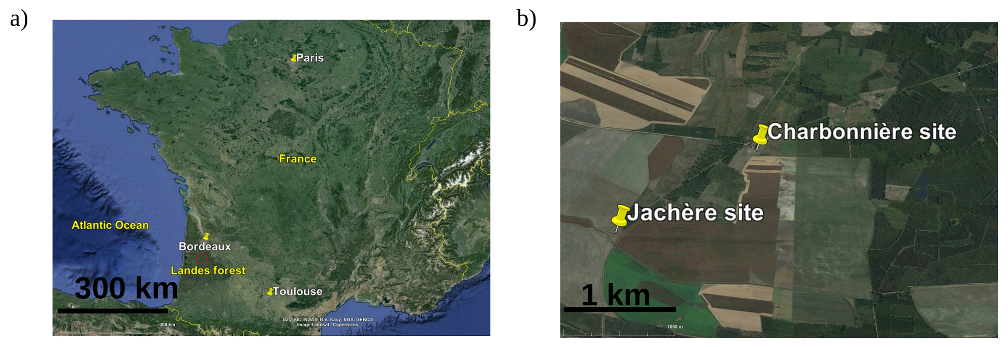
Figure 1 (a) Map of France with the location of SOFOG3D in a red rectangle (© Google Earth). (b) Focus on the Jachère and Charbonnière sites (© Google Earth).

Table 1 List of instruments used in this study. References for uncertainty are ¹ Delanoë et al. (2016), ² Martinet et al. (2022), and ³ Lance et al. (2010).

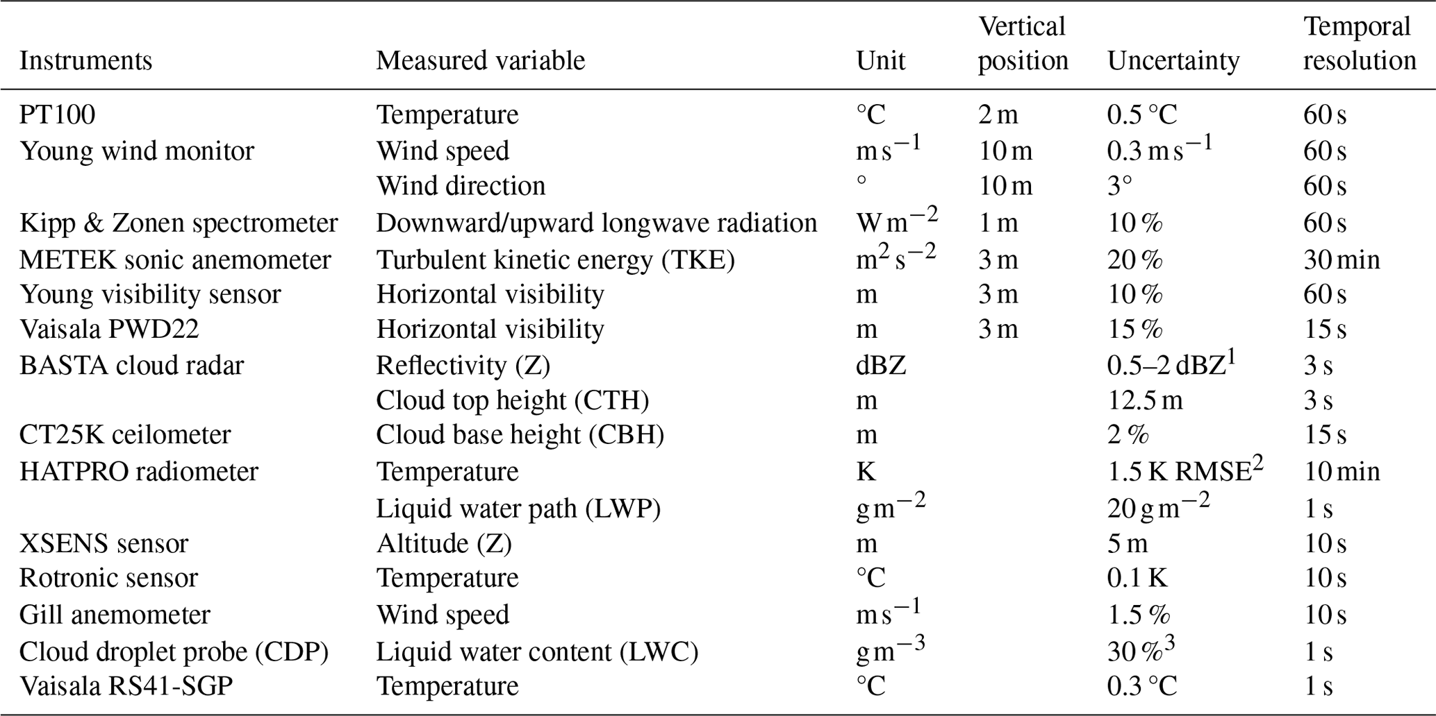
The instruments used in this study are summarized in Table 1. Both sites were equipped with a ground-based meteorological station that provided standard dynamical and thermodynamical measurements such as temperature, wind speed, wind direction, and longwave and shortwave radiation.

A 95 GHz BASTA cloud radar was operated at the Charbonnière site on a vertical pointing mode. It measured radar reflectivity and Doppler velocity up to 18 km with three vertical resolutions (12.5, 25 and 100 m) (Delanoë et al., 2016). The 12.5 m vertical-resolution mode was dedicated to fog and low clouds, with the first available gate between 25 and 37.5 m a.g.l. Cloud top height (CTH) was provided at a time resolution of 3 s, by the level-2 product developed by combining the three modes to derive optimized radar reflectivity, velocity and mask indicating the valid signal from noise. A additional mask was defined to remove radar reflectivities when the tethered balloon was interfering with the cloud radar measurements (Delanoë, 2020). Since qualitative analysis of the BASTA reflectivities is performed here to provide geometrical thickness of the fog layer, we choose to use all the available data, and this specific mask is not applied. Cloud base height (CBH) was determined using observations from a Vaisala CT25K 1/4 Hz ceilometer located at the Charbonnière site, measuring CBH for up to three cloud layers, with a vertical resolution of 15 m. An RPG HATPRO 1/10 Hz microwave radiometer (MWR) was also deployed at the Charbonnière site (Martinet et al., 2022). Using neural network inversion, it provided vertical temperature and humidity profiles up to 2.5 km with a vertical resolution of 25 m up to 100 m high and 30 m above, as well as the liquid water path (LWP) over the whole layer. The synergy between both instruments was investigated for IOP 11 (Vishwakarma et al., 2023) and IOP 14 (Bell et al., 2022), by combining the LWP retrieved from the radiometer and the reflectivity from the BASTA radar in order to better estimate the vertical profile of LWC within the fog layer. Here we analyse independently the BASTA radar and HATPRO radiometer measurements collected during 12 IOPs of the SOFOG3D experiment.

An 18 m³ tethered balloon was operated at the Charbonnière site to provide in situ measurements through the boundary layer up to 500 m during the fog events. The payload consisted of an adapted DMT cloud droplet probe (CDP) for fog microphysics and meteorological sensors to provide thermodynamical vertical profiles of temperature, humidity, wind speed and wind direction. A Gill ultrasonic anemometer and an inertial sensor were used for turbulence measurements (Canut et al., 2016), except for IOPs 6a-c during which they were replaced by a Vaisala tethersonde. The CDP is an aircraft instrument that provides the 1 Hz cloud droplet size distribution from 2 to 50 µm in diameter (Lance et al., 2010). To operate under a tethered balloon, a wind vane was used to align the sampling section perpendicular to the wind and a small fan fixed just to the rear of the laser beam sucked in the air flow. The air speed in the sampling section was therefore equal to the wind speed plus 5 m s⁻¹ (Fathalli et al., 2022).

2.2 Case studies

During the SOFOG3D campaign, 15 intensive observation periods (IOPs) with tethered balloon operations were conducted. Here we analyse 12 fog events sampled with the CDP under the balloon. Their characteristics are summarized in Table 2.

The time of formation and of dissipation and the type of fog are determined on the basis of measurements at the Jachère site since visibility measurements at the Charbonnière site were only available between 23 January and 4 March 2020. A fog event starts when visibility falls below 1 km for at least 30 min, and dissipation occurs when visibility exceeds this threshold for more than 1 h.

The algorithm developed by Tardif and Rasmussen (2007) was implemented to determine the type of fog that should reflect the main processes leading to fog formation. It depends on the magnitude of radiative cooling and wind speed, as well as the presence of precipitation or stratus cloud prior to fog formation. But threshold effects appeared for several cases, leading to fog being classified as either radiative or advective, even though these two major processes are equally important. This is because Tardif and Rasmussen (2007) considered radiative–advective fogs to be radiative fogs because no distinction was made between heating and air drainage. Given the importance of the advective component observed during SOFOG3D linked to the proximity of the Atlantic Ocean, we analysed large-scale conditions using synthetic analysis products, in addition to local conditions in the supersite's surroundings at the fog formation, using satellite data, radar and thermodynamical parameters from meteorological stations at the Jachère and Charbonnière sites. In particular, a sudden increase in longwave radiation, wind speed and specific humidity, as well as a decrease in visibility and variation in wind direction, reflecting advective processes, were analysed for each case. This analysis enabled us to determine the most appropriate classification, allowing a fog to be classified as radiative–advective (Ryznar, 1977; Gultepe et al., 2007; Yang et al., 2018) if both aspects are considered significant. All other possible fog types were the same as those described by Tardif and Rasmussen (2007) (i.e. radiative, advective, precipitation, stratus-lowering and evaporation fogs).

Three deep fog events with a CTH higher than 200 m were sampled with the tethered balloon, namely IOP 6c, 11 and 14. Given such vertical development, they have clearly undergone a transition from thin to thick. The life cycle of these cases has been examined by Dione et al. (2023) to analyse the thermodynamics and turbulent processes involved in fog formation, evolution and dissipation. Most of the fog layers sampled at the Charbonnière site, however, reached much lower thickness than these three cases. Indeed we found only one additional thick fog in the database (IOP 9a), while the other eight cases remained optically thin. For the four thick events, estimations of the onset and ending of the thin-to-thick transition are provided in Table 2 with a duration reflecting the associated uncertainty in the end of the transition based on a method described in the next section.

Table 2 Summary of the IOPs from the SOFOG3D campaign used in this study, based on the measurements at the Jachère site (except for the ending of the transition phase derived from the Charbonnière or Jachère site depending on the instrument). IOPs in bold correspond to episodes that underwent a transition from thin to thick fog. Types RAD and RAD–ADV correspond to radiation and radiation–advection fogs, respectively. Onset of the transition phase is based on Dione et al. (2023) for IOPs 11 and 14. The uncertainty in the transition phase duration, determined by the time interval between the first and last threshold of the transition ending (see text), is indicated in brackets. IOPs 13b, 14, 11 and 6c are studied more specifically in Sect. 4.

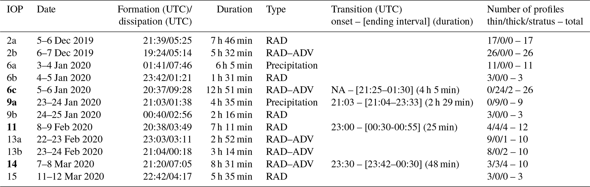
For the in situ measurements performed under the tethered balloon, the observation strategy consisted of ascents and descents through the layer to provide vertical profiles of the fog microphysics and thermodynamics and constant-height sections at various altitude to investigate time evolution and turbulence within the fog layer. To be representative, the turbulent kinetic energy (TKE) is determined over constant-height sections lasting at least 20 min. Tethered balloon tracks for the four fog events analysed in Sect. 4 are illustrated in Figs. 8c, 9c, 10c and 11c superimposed to the radar reflectivity, for IOP 13b, 14, 11 and 6, respectively. The maximum ascent or descent speed of the balloon is 0.5 m s⁻¹. It then theoretically takes 10 min to cross a 150 m thick layer. However, due to the increase in the wind with the altitude that tends to sweep off the balloon away from the winch, the required time is much higher. In addition, the CDP is powered with a battery that allows measurements up to a maximum of around 1.5 h. As a result, some profiles did not cross the entire fog layer from the ground up to the CTH and were discarded for this study. For five episodes, some vertical profiles were performed after the fog lifted into a stratus cloud during the dissipation phase, including the two thin cases sampled at the end of February. Overall a total of 140 vertical profiles were selected, including 87 in thin fogs, 40 in thick fogs, and 13 in stratus clouds. The number of profiles is given for each IOP in the last column of Table 2. The number of profiles available in each phase of the life cycle is highly variable depending on fog duration, vertical extension and various technical difficulties encountered during operations. But with the exception of three events, there are between 9 and 26 profiles per fog case, providing a unique dataset to document the vertical structure of the thermodynamics and microphysical properties of fog layers.

2.3 Determination of the thin-to-thick transition phase duration

As mentioned in Sect. 1, a fog becomes optically thick when the layer closest to the ground radiates sufficiently in the longwave range to warm the surface below. This leads to the destabilization of the fog layer, which evolves from a stable to a neutral or slightly unstable temperature profile. Precise estimation of the transition phase duration is not easy, however. Many authors have proposed various thresholds for different radiative, thermodynamic, geometric and microphysical parameters. We choose to define the onset of the transition phase on the basis of the Dione et al. (2023) study. The transition phase ending is determined by applying the following five conditions for the four thick fogs, in order to assess the uncertainty associated with the definition of the transition phase duration. This methodology allows us to evaluate whether multiple thresholds reached in a short period of time result in a rapid transition phase duration and whether large discrepancies in the ending of the transition phase can be caused by local or non-local processes.

To smooth out high-frequency fluctuations that are not representative of the typical length scale of the fog phases, we compute the transition duration ending for a given parameter from the 30 min running average of its time series except for the TKE and vertical temperature gradient for which original sampling frequency data are used (Table 1).

• As the fog becomes optically thick, the longwave net radiation LW_N= (LW_DOWN−LW_UP) increases during the night and approaches 0 (Wærsted et al., 2017; Dupont et al., 2016; Dhangar et al., 2021). Mazoyer et al. (2017) observed a difference of 8 W m⁻² between LW_DOWN and LW_UP after the fog vertical development. We consider that the transition ends when $\left|{\mathrm{LW}}_{\mathrm{N}}\right|<\mathrm{5}$ W m⁻².

• Warming at the surface and cooling at the fog top destabilize the vertical profile of temperature, which reverses from stable conditions and starts to decrease with height (Roach et al., 1976; Price, 2011). We use the temperature profile provided by the MWR just above the surface, but we have discarded the first two gates because of the excessive influence of the ground on the measurements. The considered threshold is when the temperature gradient between 50 and 25 m becomes negative, i.e. T_50 m<T_25 m.

• Due to the destabilization of the vertical temperature profile, turbulent motions increase (Nakanishi, 2000). A threshold of ${\mathit{\sigma }}_w^{\mathrm{2}}$ values is difficult to define. Price (2019), during the LANFEX campaign, proposed ${\mathit{\sigma }}_w^{\mathrm{2}}$ values higher than 0.002–0.005 m² s⁻² at the transition. But Dione et al. (2023) found much larger values ($\mathrm{0.01}<{\mathit{\sigma }}_w^{\mathrm{2}}<\mathrm{0.04}$ m² s⁻²) during the stable–adiabatic transition of the four deepest fog events of SOFOG3D and an increase in TKE of up to 0.4 m² s⁻². These discrepancies may be explained by the contrasting environment between the two measurement areas, characterized, respectively, by a complex topography for LANFEX with sites located in valleys and at hilltops and a relatively flat area at SOFOG3D with a mixture of open and forested sites (Thornton et al., 2023). In the same way, Dhangar et al. (2021), during the WIFEX campaign over New Delhi, considered a TKE threshold of 0.10 m² s⁻². We then choose TKE > 0.10 m² s⁻².

• An increase in geometrical thickness is systematically observed as the fog becomes optically thick. This vertical development can be detected using the fog cloud top height derived from cloud radars (Wærsted et al., 2017) or tethered balloon systems (Price, 2011). Based on these studies we consider that the transition ends when the CTH > 110 m.

• Finally, the LWP also increases. We apply the condition determined by Wærsted et al. (2017), i.e. LWP > 30 g.m⁻².

The optical depth, τ, increases as the fog becomes optically thick (Vehil et al., 1989). Wærsted et al. (2017) consider opaque fog when τ>5. Droplet size distribution measurements from the CDP collected during vertical profiles provide the opportunity to compute the optical depth of the fog layer:

$$\begin{array}{}\text{(1)}& \mathit{\tau }=\underset{Zb}{\overset{Zt}{\int }}{\mathit{\sigma }}_{\mathrm{ext}}\left(z\right)\mathrm{d}z,\end{array}$$

where σ_ext is the extinction, and Zb and Zt are the cloud base and cloud top heights, respectively. Optical depth from CDP measurements is computed for each of the 140 vertical profiles to provide an independent assessment of the optically thin and thick foggy periods.

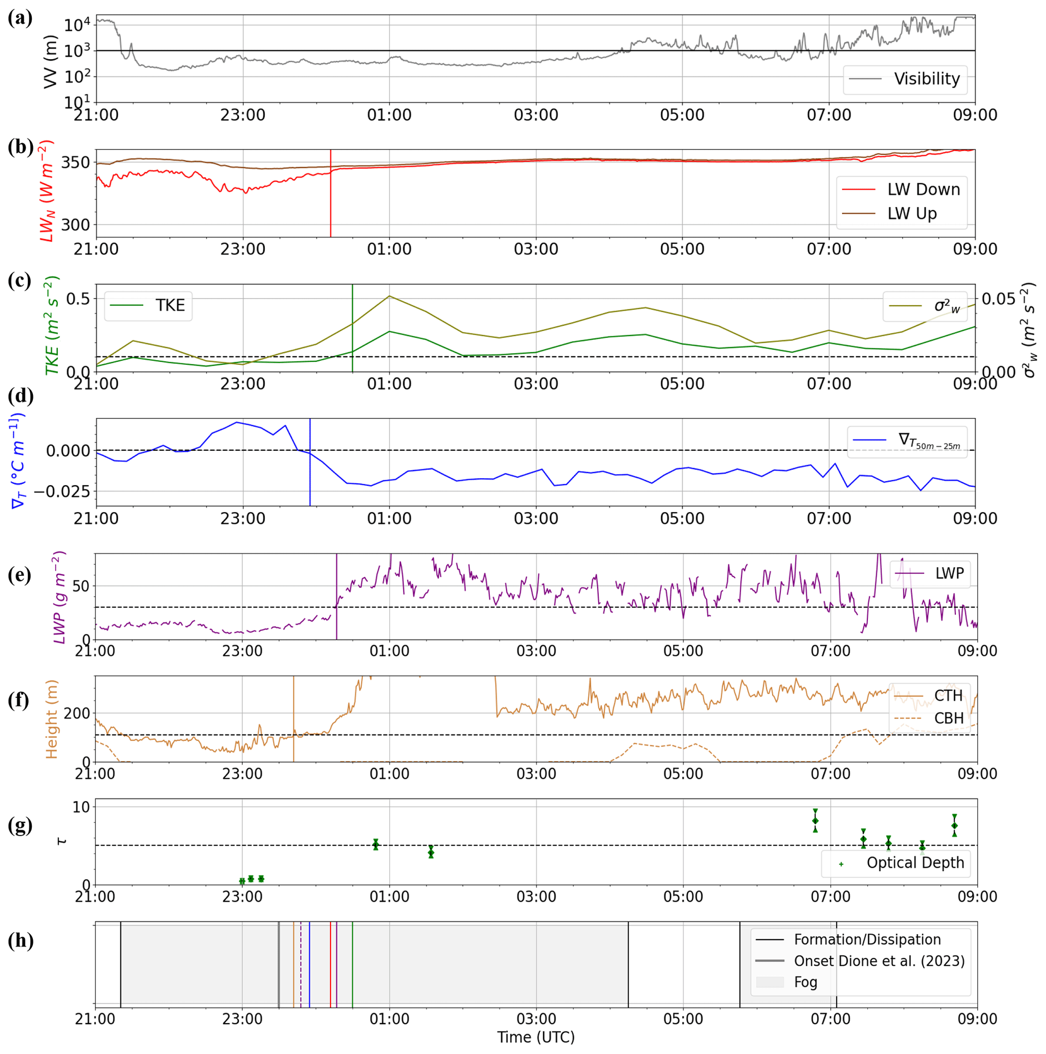
Figure 2 Time series for IOP 14 fog event: (a) visibility (b) downward (light red) and upward (brown red) longwave radiative fluxes, (c) TKE (green) and ${\mathit{\sigma }}_w^{\mathrm{2}}$ (light green), (d) vertical gradient of temperature between 25 and 50 m from the MWR, (e) LWP from the MWR, (f) CTH from the BASTA cloud radar and CBH from the ceilometer, and (g) optical depth from the CDP. In panels (c) to (g), threshold values are indicated by the dotted horizontal lines. In panels (b) to (f), the vertical segments represent the transition ending times. (h) Summary graph with the five transition ending times and their respective colours superimposed over the foggy period (grey area) delimited by the formation and dissipation times in vertical black lines. Onset of the transition phase following Dione et al. (2023) is indicated by a thick vertical grey line. The vertical dotted purple segment represents the transition ending time derived from the LWP with a threshold of 15 g m⁻² instead of 30 g m⁻². Measurements from the Charbonnière site, except visibility and TKE in panels (a) and (c) from the Jachère site.

Results for IOP 14 case study are illustrated in Fig. 2. Each transition ending time for a given parameter is represented by a vertical bar on the corresponding time series in Fig. 2b–f, and they are all reported in Fig. 2h for a synthetic representation. Optical depth (Fig. 2g) reveals low values for the first three profiles with τ<1, while it remains close to or above the threshold of 5 from profile 4. This suggests that fog becomes optically thick between 23:15 (profile 3) and 00:49 UTC (profile 4). These observations are consistent with Dione et al. (2023), who defined the onset of the transition phase at 23:30 UTC. In addition, the transition phase ending is systematically associated with an increase in LW_N, TKE, LWP and CTH and a decrease in the vertical temperature gradient. For this case, the different transition time ending values are very close within a 48 min period around midnight, leading to a short transition phase duration ranging between 12 min (CTH, orange) and 1 h (TKE, green). But there could be large discrepancies. Figure A1 presents the results for IOP 11, where Dione et al. (2023) determined the onset of the transition phase at 23:00 UTC, while ending times are distributed from 00:30 to 00:55 UTC, except the 30 g m⁻² LWP threshold about 2 h later. This threshold seems too high in this case since the transition rather ends when LWP reaches 15 g m⁻². The transition phase duration is longer for this case, from 1.5 h to 1 h and 55 min, but it is not associated with a higher uncertainty in the ending time, which is shorter than for IOP 14 (Table 2). Furthermore, we do not observe a significant increase in optical thickness during the transition phase, with values not exceeding 2 until the fog dissipates at 03:56 UTC. Indeed, we will see in Sect. 5 that these low values of optical depth while the fog is optically thick result from the sedimentation process. IOP 6 reveals the largest uncertainty in the transition phase ending (Fig. A2) with the LW flux exceeding 5 W m⁻² very early (50 min) after the fog onset, about 2.5 h before the TKE threshold and 3.5 h before both CTH and vertical temperature gradient thresholds. This appears to be mainly due to advective processes that perturbed the fog life cycle. Indeed all these parameters are also close to their respective thresholds (CTH = 87.5 m, TKE = 0.06 m² s⁻² and vertical temperature gradient = 0.0007 °C m⁻¹), but the vertical development of the fog layer is temporarily stopped as the surface wind decreased before its direction shifted from SW to SE (Fig. 11a). The fog started to deepen again around midnight, and then all parameters reached their thresholds shortly after, except the 30 g m⁻² LWP threshold, which required 1 h and 15 min more. The optical depth follows a similar evolution with values close to 2 shortly after fog formation, decreasing to 0.32 and 0.21 for profiles 4 and 5, respectively, around 23:00 UTC, when the vertical development is stopped, and increasing again after midnight during the second vertical development, with values up to 6. The threshold of 5 seems then too high since values are closer to 2 when fog is optically thick shortly after fog formation. Dione et al. (2023) defined the onset of the transition phase at 00:00 UTC, which actually corresponds to the second period of thick fog. Consequently, for this case, the onset remained undefined. This illustrates the difficulty in defining accurate thresholds for complex fog life cycles. Finally, during IOP 9a (not shown), which was not examined by Dione et al. (2023), LW_N indicates that the fog is already thick at its formation, due to the immediate condensation of liquid water over a 80 m thick layer but with a rather low value of LWP < 5 g m⁻². A cloud passing above temporarily caused the fog layer to drop below 50 m, and as for IOP 6, other parameters then exceed their thresholds later on when the fog started to deepen again, resulting in a transition ending time uncertainty of 2 h and 29 min, as indicated in Table 2.

For these four cases, transition phase ending occurred with LWP values systematically much lower than the 30 g m⁻² threshold. To be consistent with the other parameters, we find that a value of 15 g m⁻² is more suited to detect the transition ending. The other estimations are in agreement during IOPs 11 and 14, during which there was a clear thin-to-thick transition phase ending period shorter than 1 h, but they are more dispersed during IOPs 9a and 6c while the fog became optically thick immediately after its formation or shortly after, respectively. As a result, no tendency is observed between the time interval during which the different thresholds are reached and the duration of the transition period. This suggests that multiple thresholds reached in a short period of time do not seem to favour a rapid thin-to-thick transition and, conversely, that a slow transition is not systematically associated with inconsistencies between all the thresholds. In addition, these four cases do not reveal any trend in the order of exceeding the thresholds by the different parameters. Furthermore it appears that non-local processes such as the change in wind orientation or the advection of clouds can disrupt the usual fog life cycle by stopping the vertical development of the fog layer. Finally, evolution of the optical depth revealed a strong increase at the transition during IOP 14, while lower values are found for IOPs 11 and 6. The threshold of 5 appears then too high, and we find that a value of 2 is more appropriate to discriminate between optically thin and thick fogs. Note that this value is consistent with retrievals reported by Guy et al. (2023) from spectral measurements of downwelling longwave radiation performed with the Atmospheric Emitted Radiance Interferometer (AERI). For the 12 optically thin fogs sampled in central Greenland, including 9 mixed-phase cases, most of the 5 min liquid and ice optical depth retrievals are much lower than 2, with median values of 0.8 and 0.5, respectively.

This analysis provides estimations of the transition phase duration for each case with an associated period of uncertainty, independent of the in situ measurements performed under the tethered balloon. These are now examined to document the evolution of the vertical profile of microphysical properties during the fog life cycle, with particular emphasis on fog adiabaticity.

3 Fog adiabaticity

3.1 Equivalent adiabaticity from closure and parameterization as a function of CTH

In adiabatic liquid clouds, the liquid water content increases almost linearly with the altitude as LWC$\left(z\right)={\mathrm{\Gamma }}_{\mathrm{ad}}(T,P)(z-Zb)$, where Γ_ad(T,P) is the condensation rate that depends on pressure P and temperature T at the cloud base (Betts, 1982; Albrecht et al., 1990; Brenguier, 1991) following

$$\begin{array}{}\text{(2)}& {\mathrm{\Gamma }}_{\mathrm{ad}}(T,P)={\mathit{\rho }}_{\mathrm{d}}({\displaystyle \frac{(\mathit{ϵ}+w_{\mathrm{s}})w_{\mathrm{s}}{l}_v{\mathrm{\Gamma }}_w}{R_{\mathrm{d}}{T}^{\mathrm{2}}}}-{\displaystyle \frac{g{w}_{\mathrm{s}}P}{(P-e_{\mathrm{s}})R_{\mathrm{d}}T}}),\end{array}$$

with l_v the latent heat of vaporization, g the acceleration of gravity, R_d the dry-air ideal gas constant, ϵ the ratio between the dry air to water vapour ideal gas constant equal to 0.622, e_s the vapour saturation pressure, w_s the saturation mixing ratio, ρ_d the dry-air density, and Γ_w the moist adiabatic lapse rate given in Eq. (3) (Hummel and Kuhn, 1981).

$$\begin{array}{}\text{(3)}& {\mathrm{\Gamma }}_w={\displaystyle \frac{g}{c_{\mathrm{p}}}}{\displaystyle \frac{\mathrm{1}+\frac{l_v{w}_{\mathrm{s}}}{R_{\mathrm{d}}T}}{\mathrm{1}+\frac{\mathit{ϵ}{l}_v^{\mathrm{2}}{w}_{\mathrm{s}}}{R_{\mathrm{d}}{c}_{\mathrm{p}}{T}^{\mathrm{2}}}}},\end{array}$$

with c_p the specific heat of dry air at constant pressure.

The liquid water path of a cloud layer is the total amount of liquid water:

$$\begin{array}{}\text{(4)}& \mathrm{LWP}=\underset{Zb}{\overset{Zt}{\int }}\mathrm{LWC}\left(z\right)\mathrm{d}z.\end{array}$$

In shallow convective clouds where the condensation rate can be assumed relatively constant, it follows Albrecht et al. (1990): LWP${}_{\mathrm{ad}}=\frac{\mathrm{1}}{\mathrm{2}}{\mathrm{\Gamma }}_{\mathrm{ad}}(T,P)(Zt-Zb{)}^{\mathrm{2}}$.

Processes such as entrainment mixing of dry air or precipitation formation, however, tend to reduce LWC values, and Betts (1982) introduced the in-cloud mixing parameter β to reduce the condensation rate as $(\mathrm{1}-\mathit{\beta }){\mathrm{\Gamma }}_{\mathrm{ad}}(T,P)$. Many studies have quantified departure from the adiabatic values using aircraft in situ data and revealed that the reduction in stratiform clouds is much lower than in cumulus ones and results mainly from mixing at the cloud top and drizzle formation (Gerber, 1996; Wood, 2005; Brenguier et al., 2011; Braun et al., 2018). By using remote sensing instruments in shallow stratocumulus clouds, Albrecht et al. (1990) also noticed a large reduction in LWP, compared to the adiabatic values, when drizzle is observed. Observations in fog are rare due to the difficulty of measurement, but previous studies have reported LWC profiles that are fairly constant or increase with height in a well-developed fog layer (Okita, 1962; Pinnick et al., 1978; Price et al., 2015; Egli et al., 2015).

To retrieve the cloud base from satellite data, allowing discrimination between low stratus and fog, Cermak and Bendix (2011) developed a subadiabatic model of cloud microphysics. They derived a complex cloud profile parameterization used for LWP computation by dividing the cloud in three layers with different β values to account for processes reducing the LWC near the ground, in the central region and at the cloud top.

Recently, to improve nowcasting of fog dissipation, Toledo et al. (2021) developed a one-column conceptual model of adiabatic continental fog by assuming that the LWC linearly increases with height with a reduced condensation rate expressed as α(z)Γ_ad(T,P), where α(z) is the local adiabaticity. The LWP of a fog layer is then computed considering that the equivalent adiabaticity ${\mathit{\alpha }}_{\mathrm{eq}}=\mathrm{1}-\mathit{\beta }$ remains constant throughout the fog layer from the ground to the CTH:

$$\begin{array}{}\text{(5)}& \mathrm{LWP}={\displaystyle \frac{\mathrm{1}}{\mathrm{2}}}{\mathit{\alpha }}_{\mathrm{eq}}{\mathrm{\Gamma }}_{\mathrm{ad}}(T,P)\cdot {\mathrm{CTH}}^{\mathrm{2}}+{\mathrm{LWC}}_{\mathrm{0}}\cdot \mathrm{CTH},\end{array}$$

where LWC₀ is the LWC value at the ground.

Toledo et al. (2021) then used data from 7 years of measurements performed at the SIRTA (Site Instrumental de Recherche par Télédétection Atmosphérique) observatory near Paris, to compute this equivalent adiabaticity α_eq. Without measurements of the vertical profiles of LWC, they used an inversion of Eq. (5) to calculate α_eq by closure:

$$\begin{array}{}\text{(6)}& {\mathit{\alpha }}_{\mathrm{eq}}^{\mathrm{closure}}={\displaystyle \frac{\mathrm{2}(\mathrm{LWP}-{\mathrm{LWC}}_{\mathrm{0}}\cdot \mathrm{CTH})}{{\mathrm{\Gamma }}_{\mathrm{ad}}(T,P)\cdot {\mathrm{CTH}}^{\mathrm{2}}}},\end{array}$$

where LWP and CTH are provided by a HATPRO MWR and a BASTA radar, respectively, and LWC₀ is derived from the measured visibility at ground level by the parameterization developed in Gultepe et al. (2006).

${\mathit{\alpha }}_{\mathrm{eq}}^{\mathrm{closure}}$ is then the equivalent adiabaticity that would give the same LWP in the fog layer but assuming a linear increase in LWC with height. Note that from Eq. (6), ${\mathit{\alpha }}_{\mathrm{eq}}^{\mathrm{closure}}=\mathrm{0}$ corresponds to a constant LWC profile equal to LWC₀ from the ground to CTH and is quite different from β=1, which corresponds to the total evaporation of the cloud due to mixing with clear air (Betts, 1982). Toledo et al. (2021) found that ${\mathit{\alpha }}_{\mathrm{eq}}^{\mathrm{closure}}$ depends mainly on the CTH, converging to ≈0.7 for developed fogs, and pointed out that thinner fog with LWP values lower than 20 g m⁻² has ${\mathit{\alpha }}_{\mathrm{eq}}^{\mathrm{closure}}$ values below 0.6 and can even reach negative values. They thus proposed the following parameterization:

$$\begin{array}{}\text{(7)}& {\mathit{\alpha }}_{\mathrm{eq}}\left(\mathrm{CTH}\right)={\mathit{\alpha }}_{\mathrm{0}}(\mathrm{1}-e^{-\frac{\mathrm{CTH}-H_{\mathrm{0}}}{L}}),\end{array}$$

where α₀=0.65, H₀=104.3 m and L=48.3 m.

Dione et al. (2023) used this parameterization to analyse the four deepest fogs of SOFOG3D. They revealed negative values of α_eq (CTH) during the stable phase, which increase from 0 to 0.5 during the thin-to-thick transition and finally exceed 0.5 when LWP > 20 g m⁻². Therefore, analysis of α_eq (CTH) enables the discrimination between optically thin and thick fog, characterized by negative and positive values, respectively.

Note that negative adiabaticity values result mathematically from high LWC₀ values at the surface and low LWP of the fog layer. This reflects that the LWC profile is not increasing with height and consequently that the basic assumption of the conceptual model is not valid. We now use the CDP measurements to analyse fog adiabaticity derived from in situ measurements.

3.2 Vertical profiles of LWC and temperature from in situ measurements

Droplet size distribution recorded by the CDP under the tethered balloon during SOFOG3D allows us to retrieve vertical profiles of LWC in the fog layer and then to examine the actual fog adiabaticity and compare it to the equivalent values derived by closure.

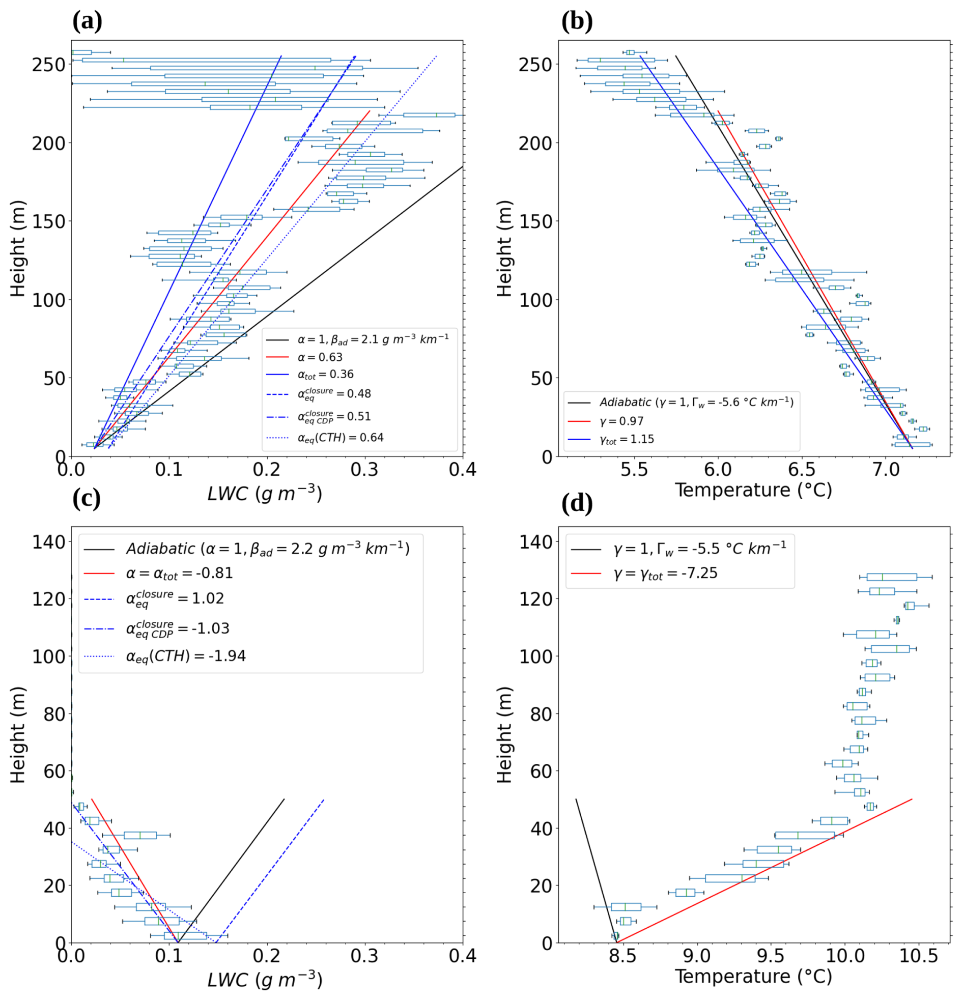
Figure 3 Vertical profiles of (a, c) LWC and (b, d) temperature measured during (a, b) a descent of IOP 14 between 06:11 and 06:47 UTC and (c, d) a descent of IOP 11 between 22:09 and 22:23 UTC. Boxplots are derived from data collected within 5 m height layer. Adiabatic values are indicated by a black line. Adiabaticity calculated over the entire profile and adiabaticity over the profile truncated at the altitude of the maximum of LWC are indicated by a solid blue and a red line, respectively. The equivalent adiabaticity from closure (Eq. 6) retrieved by remote sensing $({\mathit{\alpha }}_{\mathrm{eq}}^{\mathrm{closure}}$) and in situ measurements (${\mathit{\alpha }}_{\mathrm{eqCDP}}^{\mathrm{closure}}$) are indicated by a dashed and dash-dotted blue line, respectively, while the equivalent adiabaticity derived from the parameterization as a function of CTH (Eq. 7) is indicated by a dotted blue line.

Figure 3 presents vertical profiles of LWC and temperature measurements collected during IOP 14 (upper panels) and IOP 11 (lower panels). Boxplots correspond to statistics computed within 5 m height layers from the ground up to the fog top. Black lines indicate the adiabatic theoretical calculation of LWC and lapse rate, from Eqs. (2) and (3), respectively.

The ascent of IOP 14 was performed between 06:11 and 06:47 UTC, about 6 h after the fog became optically thick (Fig. 2) and 2 h before its dissipation in stratus (profile 6 of Fig. 9d). As a general trend, LWC values increase with the altitude up to 215 m, before they drop suddenly in the upper fog layers near the fog top at 255 m (Fig. 3a). In this deep fog, however, we can observe that the increase in LWC is not continuously monotonic, with the presence of a layer with much lower LWC values at heights between 120 and 170 m. The vertical profile of temperature decreases almost regularly with height up to the fog top (Fig. 3b). Unfortunately, the balloon failed to cross the summit due to the increase in wind speed to over 6 m s⁻¹, but the radiosonde launched 35 min earlier indicates a sharp temperature inversion of −1.5 °C (not shown). These observations are consistent with previous measurements in well-mixed fog layers revealing mainly adiabatic vertical profiles of LWC and temperature, as well as a sharp reduction in LWC at the fog top, probably due to entrainment mixing of dryer air in the upper fog layers.

In contrast, the descent during IOP 11 between 22:09 and 22:23 UTC reveals a reverse trend with LWC being maximal at the ground, around 0.11 g m⁻³, and decreasing with altitude up to the CTH at 55 m, except a thin slice around 40 m. It is associated with a stable vertical profile of temperature that increases from 8.5 °C at the ground to 10.1 °C above the CTH. Indeed at this time (profile 2 of Fig. 10d) the fog is still optically thin as the transition to thick fog will occur about 1.5 h later. Such reverse LWC profiles were almost systematically observed in optically thin fogs during the SOFOG3D campaign and are investigated in more detail in Sect. 4. These results highlight contrasting vertical profiles between well-mixed fogs, whose characteristics can be correctly represented by the adiabatic model, and thin fogs exhibiting an opposite trend.

For LWC profiles, the linear increase corresponding to ${\mathit{\alpha }}_{\mathrm{eq}}^{\mathrm{closure}}$ calculated from Eq. (6) following Toledo et al. (2021) is plotted as a dashed blue line with values of 0.48 and 1.02 for IOP 14 and IOP 11, respectively. It is worth noting that these values differ from the values of α_eq (CTH) derived from the parameterization as function of CTH (Eq. 7) used by Dione et al. (2023). As expected for the well-mixed fog case, the resulting profile of LWC tends to underestimate actual values of LWC in the lower part of the layer with predicted values that can be half the measured ones. The dotted and long dashed blue line corresponds to the fog adiabaticity from closure but computed with the CDP data ${\mathit{\alpha }}_{\mathrm{eqCDP}}^{\mathrm{closure}}$ (see next section) and produces a very similar result. Indeed, these low values of ${\mathit{\alpha }}_{\mathrm{eq}}^{\mathrm{closure}}$ result mainly from the strong reduction of LWC at the fog top. Consequently, the corresponding profiles of ${\mathit{\alpha }}_{\mathrm{eq}}^{\mathrm{closure}}$ are not really representative of the global agreement of the measured LWC with the adiabatic model. An overall agreement is, however, clearly reflected in the temperature (Fig. 3b), the adiabaticity (blue) being less affected by the evaporation following the mixing below the fog top. The profile of α_eq (CTH), represented by a dotted blue line, enables one to retrieve an equivalent adiabaticity more in agreement with the general trend of LWC with altitude. The value of 0.64 is close to the asymptote of the parameterization (α₀=0.65) due to a high CTH reaching 255 m. Surprisingly, the reverse LWC profile of IOP 11 is well reproduced with data aligned along the negative slope −1.03 of ${\mathit{\alpha }}_{\mathrm{eqCDP}}^{\mathrm{closure}}$. In contrast for this case, ${\mathit{\alpha }}_{\mathrm{eq}}^{\mathrm{closure}}$ is positive due to a larger LWP value provided by the MWR (7.12 g m⁻²) compared to the CDP measurements (2.67 g m⁻²), and the profile is shifted to larger LWC due to a larger value of LWC₀ provided by the parameterization of Gultepe et al. (2006) (0.15 g m⁻³) compared to the CDP measurements (0.11 g m⁻³). In addition, α_eq (CTH) reveals a negative value of −1.94, in agreement with ${\mathit{\alpha }}_{\mathrm{eqCDP}}^{\mathrm{closure}}$ and the general trend of LWC with height, related to a low CTH value of 55 m. These observations indicate that for optically thin fogs characterized by low LWP values (LWP < 10 g m⁻²), uncertainties in LWP measurements and LWC₀ retrievals induce inconsistencies between LWP, CTH and LWC₀ values, which implies that the closure conditions required for the calculation of ${\mathit{\alpha }}_{\mathrm{eq}}^{\mathrm{closure}}$ are not satisfied.

To better estimate the agreement of the measurements with the adiabatic model, we calculate the adiabaticity parameters α and γ with respect to LWC and lapse rate, respectively, by determining the slope of the linear regression between median values of the statistics at each altitude range and dividing by Γ_ad and Γ_w, respectively. To avoid underestimation of adiabaticity resulting from entrainment-mixing processes below the fog top for well-mixed fog, we discard this layer by truncating the vertical profile at the altitude where LWC reaches its maximum value. The corresponding profiles are superimposed as red lines in Fig. 3a and b. With such a procedure α=0.63 for IOP 14, close to α_eq (CTH), and the corresponding fit to the measurements better represents the general shape of the vertical profile than ${\mathit{\alpha }}_{\mathrm{eq}}^{\mathrm{closure}}$ and ${\mathit{\alpha }}_{\mathrm{eqCDP}}^{\mathrm{closure}}$. In addition, taking into account the entrainment-mixing layer above 220 m strongly reduces the adiabaticity to α_tot=0.36 (solid blue line). Thus, the adiabaticity derived by truncating the entrainment-mixing layer for well-mixed buoyant fogs seems to be a relevant metric to characterize the global deviation of the LWC profile from the adiabatic one. For the lapse rate γ=0.97, which is then very close to the adiabatic decrease. In contrast, the descent during IOP 11 reveals negative α and γ values of −0.81 and −7.25, respectively.

In a first step, we take advantage of the 140 selected profiles to evaluate the agreement between ${\mathit{\alpha }}_{\mathrm{eq}}^{\mathrm{closure}}$, α_eq (CTH) and the equivalent values derived from in situ data.

3.3 Comparison between equivalent fog adiabaticity estimations

For each vertical profile, ${\mathit{\alpha }}_{\mathrm{eq}}^{\mathrm{closure}}$ is computed from Eq. (6) by using the median values over the duration of the profile of CTH from the radar, LWP from the MWR and visibility measurements. Due to an instrument failure, data from the visibilimeter deployed at the Charbonnière site were only available for IOPs 9a to 13b. As for the other seven IOPs, the visibilimeter at the Jachère site (at 1.4 km) must be used. To compute the fog adiabaticity from closure with CDP data (${\mathit{\alpha }}_{\mathrm{eqCDP}}^{\mathrm{closure}}$), CTH is determined by using an LWC threshold of 0.01 g m⁻³, the LWP is calculated by integrating the median value of LWC in each altitude range up to CTH, and LWC₀ is defined as the median value of LWC in the lowest altitude range. The median height corresponding to LWC₀ is 3.5 m with first and third quartiles of 2.5 and 6.2 m, respectively, i.e. very close to the height of the visibilimeters deployed at 3 m above ground level but over a short time period typically of about 10 s. Except for CTH_CDP, the first and third quartiles of the distribution of each parameter are calculated for each vertical profile, to assess the variability during the corresponding time interval.

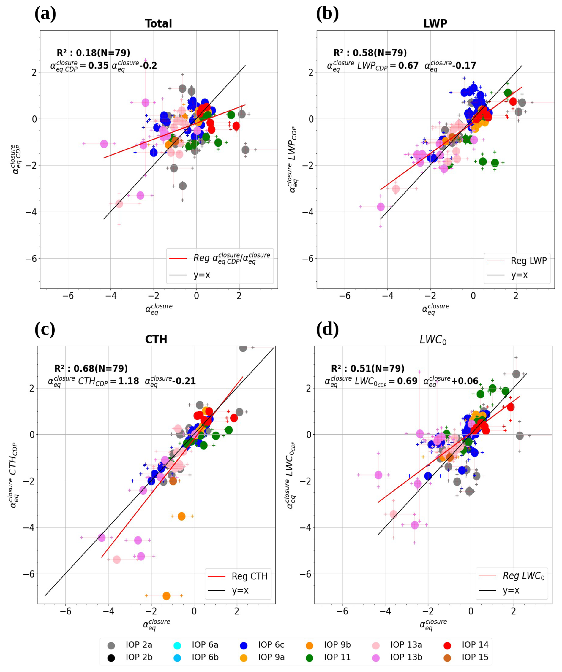
Figure 4 Fog adiabaticity from closure values comparison: (a) ${\mathit{\alpha }}_{\mathrm{eq}}^{\mathrm{closure}}$ values derived from the CDP measurements as a function of ${\mathit{\alpha }}_{\mathrm{eq}}^{\mathrm{closure}}$. Sensitivity tests performed on ${\mathit{\alpha }}_{\mathrm{eq}}^{\mathrm{closure}}$ using only one parameter derived from CDP measurements: (b) LWP, (c) CTH and (d) LWC₀. The dots and crosses correspond to the mean and the first and third quartiles of the distribution for each profile. Each IOP is represented by a specific colour, as indicated in the legend.

Comparisons of ${\mathit{\alpha }}_{\mathrm{eqCDP}}^{\mathrm{closure}}$ vs. ${\mathit{\alpha }}_{\mathrm{eq}}^{\mathrm{closure}}$ are reported in Fig. 4a and reveal large discrepancies, with very low values of the coefficient of determination R² and the slope of the linear regression, which reach 0.18 and 0.35, respectively. The first available gate of the radar being 37.5 m, it obviously cannot detect CTH below this height. In total 21 profiles performed by the tethered balloon are lower than this limit, which is about 20 % of the dataset. This provides additional motivation to compute ${\mathit{\alpha }}_{\mathrm{eqCDP}}^{\mathrm{closure}}$ in order to evaluate the conceptual approach against the actual vertical profile for the thin layers, which correspond to the formation phases of many radiation fog events in stable conditions. For LWP retrieved from the MWR measurements, caution should be taken when clouds above the fog layer are detected, because it is not possible to dissociate the LWP values of the fog layer and of the cloud layer above. Therefore, due to the presence of clouds above fog during IOP 2b and IOP 6a, these two cases were discarded. Finally, profiles within stratus cloud have also been removed to allow calculation of ${\mathit{\alpha }}_{\mathrm{eq}}^{\mathrm{closure}}$. In total the dataset is then reduced to 79 profiles. Note that both methods lead to values of ${\mathit{\alpha }}_{\mathrm{eq}}^{\mathrm{closure}}>\mathrm{1}$ but not for the same cases. This suggests that such values result from inaccuracy in measurements rather than reflecting superadiabatic conditions.

Sensitivity tests are carried out on LWP, CTH and LWC₀, by modifying only one of the three variables in Eq. (6) using the CDP measurements, the other two remaining based on the ${\mathit{\alpha }}_{\mathrm{eq}}^{\mathrm{closure}}$ calculation in order to determine which parameters introduce the most dispersion in the comparison. Discrepancies seem less related to CTH as the sensitivity test on this variable presents a satisfactory correlation with an R² value of 0.68 (Fig. 4c). For this parameter, for which no variability from the CDP measurements can be calculated, the worst cases, from IOP 9b and 13b, are mainly due to overestimation of CTH by the radar for actual CTH just above its detection limit that results in overestimation of ${\mathit{\alpha }}_{\mathrm{eq}}^{\mathrm{closure}}$. Then, the sensitivity test on LWP shows a lower but correct correlation with an R² value of 0.58 (Fig. 4b). Indeed comparison of LWP provided by the MWR to the CDP measurements reveals a very good agreement for values below 15 g m⁻², but some differences are observed for well-mixed fogs characterized by the highest LWP values (not shown). The worst cases in Fig. 4b (two green points) correspond to the IOP 11 profiles with LWP from CDP much lower than the MWR value and highlight the impact of such a difference. Note that the variability represented by first and third quartiles is relatively small compared to the dispersion and similar for both estimates, indicating that the temporal variability of LWP during the profile does not have a significant impact on the derived value of adiabaticity by closure. Finally, large differences are observed when LWC₀ is replaced by the CDP values: Fig. 4d shows that there is a strong increase in the scatter of the data, consistent with a poor value of the coefficient of determination of 0.51. Indeed, the comparison of LWC₀ values is reported in Fig. 5, which reveals large discrepancies with a coefficient of determination as low as 0.42. The slope of the regression is 0.63 (Fig. 5), but this likely results from the large scatter of the data, and it is not clear that the parameterization of Gultepe et al. (2006) with visibility measurements tends to produce systematically LWC values larger than the CDP measurements. Part of the discrepancies could arise from temporal fluctuations of LWC₀ during the time taken by the balloon to complete each profile, which cannot be truly inferred from the CDP measurements. It is also likely that the use of the visibility measurement from the Jachère site for 7 out of the 12 IOPs studied contributes to the dispersion. Therefore, these sensitivity tests reveal that the discrepancies between ${\mathit{\alpha }}_{\mathrm{eq}}^{\mathrm{closure}}$ and ${\mathit{\alpha }}_{\mathrm{eqCDP}}^{\mathrm{closure}}$ arise both from the LWC₀ values derived from visibility measurement and by differences in LWP between the CDP and the MWR. Note also that the data in Fig. 4a are not completely distributed in the same way as in Fig. 4b and d, reflecting that some differences between the parameters compensate for each other.

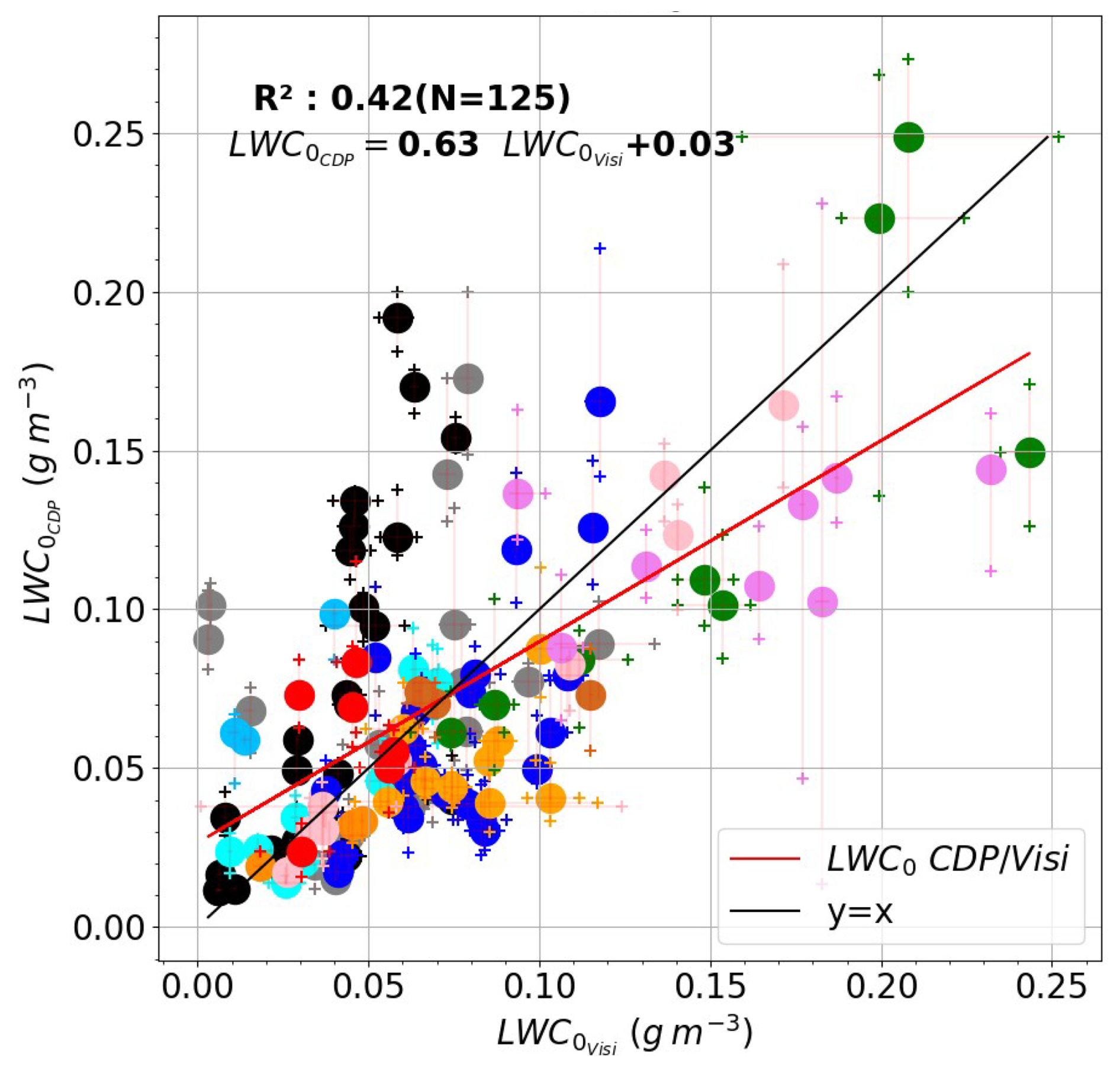
Figure 5 LWC₀ derived from the CDP measurements as a function of LWC₀ derived from the visibility measurements at the Jachère site using the parameterization defined in Gultepe et al. (2006). The dots and crosses correspond to the mean and the first and third quartiles of each profile. Each IOP is represented by a specific colour (see legend in Fig. 4).

Toledo et al. (2021) have shown the dependency of ${\mathit{\alpha }}_{\mathrm{eq}}^{\mathrm{closure}}$ on LWP and CTH, for which a parameterization as a function of CTH was proposed (Eq. 7). We therefore examined evolution of ${\mathit{\alpha }}_{\mathrm{eqCDP}}^{\mathrm{closure}}$ as a function of LWP and CTH issued from the CDP measurements for our dataset in Fig. 6, where measurements in stratus clouds have been excluded for consistency with previous studies. The observations reveal a similar trend with mainly negative values of ${\mathit{\alpha }}_{\mathrm{eqCDP}}^{\mathrm{closure}}$ when LWP < 5 g m⁻², which represents 67 % of the sampled profiles. Note that some values reach −4, much lower than those reported in Toledo et al. (2021). Indeed they correspond to very thin layers with CTH in the blind zone of the radar BASTA. Except for two profiles of IOP 11 (green dots), ${\mathit{\alpha }}_{\mathrm{eqCDP}}^{\mathrm{closure}}$ is always positive when LWP exceeds 10 g m⁻². Surprisingly, these two profiles of IOP 11 correspond to large values of CTH (Fig. 6b). Indeed we will see in Sect. 5 that these particular reverse profiles of LWC result from the sedimentation process. Beyond a LWP of 15 g m⁻², ${\mathit{\alpha }}_{\mathrm{eqCDP}}^{\mathrm{closure}}$ tends to converge around 0.5, but the number of samples is too limited for a precise evaluation of this limit. Two cases from IOP 2a exhibit superadiabatic conditions with ${\mathit{\alpha }}_{\mathrm{eqCDP}}^{\mathrm{closure}}>\mathrm{1}$. In fact, these profiles correspond to a particular case where the condensation of liquid water at the fog formation occurred first at altitude before the surface, which therefore distorts the slope calculation (see Fig. C1).

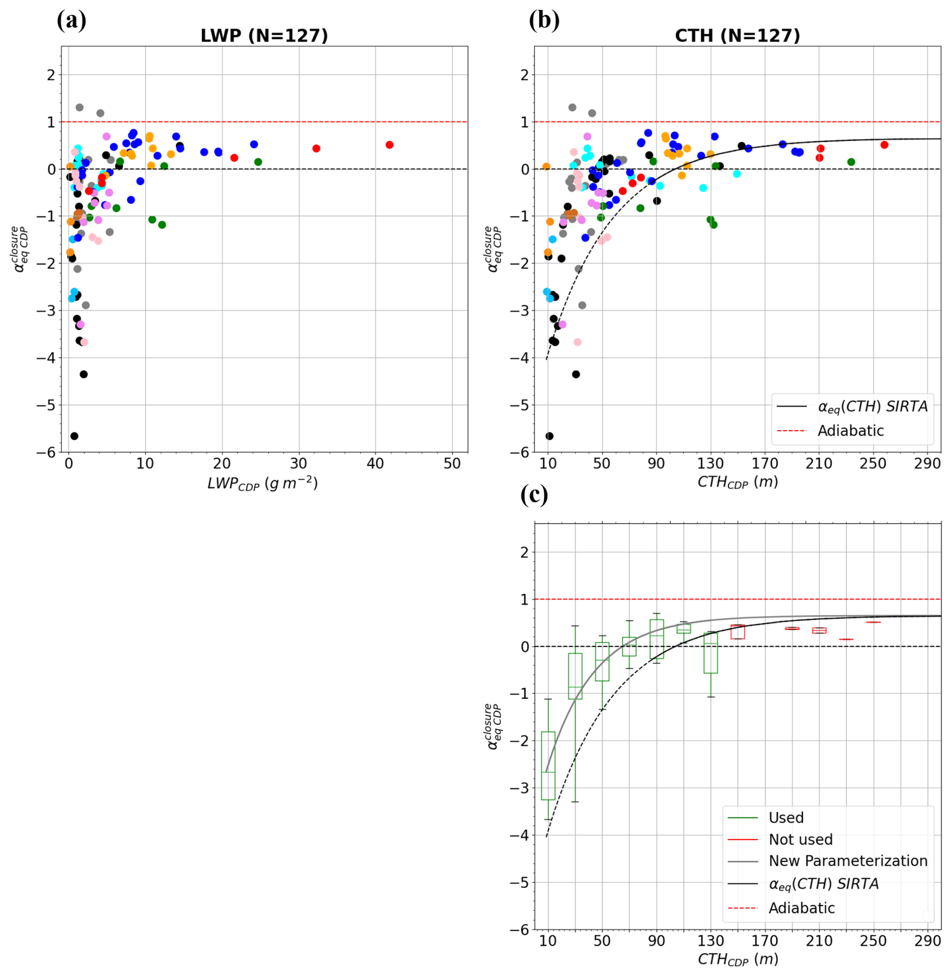
Figure 6 Equivalent adiabaticity from closure derived from CDP as a function of (a) LWP and (b) CTH. Each IOP is indicated by a specific colour, as indicated in the legend of Fig. 4. (c) Boxplot of ${\mathit{\alpha }}_{\mathrm{eq}\mathrm{CDP}}^{\mathrm{closure}}$ for each CTH range of 20 m. The parameterization of Toledo et al. (2021) and the new one based on the SOFOG3D observations are superimposed by a black and grey curve, respectively. The samples used in the new parameterization are indicated by green boxplots; those not used are indicated by red boxplots. The extension of the parameterization of Toledo et al. (2021) outside its range of validity is represented by a dashed line. The red line marks the adiabatic value.

The evolution of ${\mathit{\alpha }}_{\mathrm{eqCDP}}^{\mathrm{closure}}$ as a function of CTH depicted in Fig. 6b is very similar. The parameterization of Toledo et al. (2021) has been defined for CTH > 85 m, corresponding to the first gate of the radar used at the SIRTA site. This limit has been extended here to 10 m (dashed line) to compare with in situ data: most of them are located above this curve, reflecting that positive values of ${\mathit{\alpha }}_{\mathrm{eqCDP}}^{\mathrm{closure}}$ can be observed for a CTH lower than 85 m. Statistics on classes of 20 m width indicate that the median of ${\mathit{\alpha }}_{\mathrm{eqCDP}}^{\mathrm{closure}}$ values is positive when CTH > 70 m (Fig. 6c). For CTH > 150 m, ${\mathit{\alpha }}_{\mathrm{eqCDP}}^{\mathrm{closure}}$ values fluctuate around 0.4. This limit is lower than the convergence values of 0.65 and 0.6 reported for fog conditions in Toledo et al. (2021) and Dione et al. (2023), respectively. However, the number of profiles sampled in such developed fogs is obviously too limited here to derive significant convergence. Note that calculations of ${\mathit{\alpha }}_{\mathrm{eq}}^{\mathrm{closure}}$ with remote sensing measurements for the same profiles exhibit the same trend and do not improve the convergence estimation (Fig. B1). This attests that lower values of ${\mathit{\alpha }}_{\mathrm{eq}}^{\mathrm{closure}}$ for well-mixed deep fogs in our dataset do not result from the type of instrument used to compute adiabaticity from closure (in situ or remote sensing) but reflect the actual properties of the fogs sampled during SOFOG3D. Following Toledo et al. (2021) a parameterization of α_eq as a function of CTH is derived by minimizing Eq. (7) with respect to the median value of α_eq for each CTH range of 20 m. Only intervals with more than five valid samples are used. Given the lack of valid samples for CTH > 140 m (Fig. 6c, green boxplots), the α₀ asymptotic value is set to 0.65 as determined by Toledo et al. (2021). Thus, only the parameters H₀ and L from Eq. (7) are determined, which represent the typical CTH values at which LWC increases with height (α_eq=0) and at which the thin-to-thick transition begins (α_eq=0.5), respectively. The retrieved values, H₀=65.3 m and L=34.8 m, are lower than the values obtained by Toledo et al. (2021), 104.3 and 48.3 m, respectively. Therefore, the thinner fog layers sampled during SOFOG3D suggest that fog becomes optically thick at lower CTH than previously derived from SIRTA observations.

In summary, the comparison of equivalent fog adiabaticity from closure calculations reveals that, despite the large variability that results mainly from LWC₀ and LWP retrievals, the distribution of equivalent fog adiabaticity is approximately the same between in situ or remote sensing measurements and the Toledo et al. (2021) approach. Additionally, in situ data allow the characterization of large negative ${\mathit{\alpha }}_{\mathrm{eq}}^{\mathrm{closure}}$ values relative to thin fogs, for which a new parameterization as a function of CTH has been proposed. We now focus on in situ CDP data to examine relationships of equivalent fog adiabaticity with the actual adiabaticity.

3.4 Comparison between α, ${\mathit{\alpha }}_{\mathrm{eq}}^{\mathrm{closure}}$ and α_eq (CTH)

We introduced in Sect. 3.2 a calculation of the adiabaticity α by fitting CDP measurements (red lines in Fig. 3a, c). The diluted layer just below the top is not taken into account to represent the general shape of the LWC vertical profiles. The main objective is now to derive a synthetic parameter to better quantify departure from the adiabatic model and document its evolution during the fog life cycle. To perform a quantitative evaluation of this parameter, we extend the analysis to the 140 selected profiles of the campaign. The thermodynamical and microphysical properties of each vertical profile are calculated with a vertical resolution of 5 m for episodes that experienced thin-to-thick transition. For fogs that remained thin and very thin (less than 10 m) throughout their life cycle, the vertical resolution is increased to 3 and 1 m, respectively. Except for very thin fog episodes, the minimum number of 1 Hz CDP samples required to calculate the statistics over each altitude range was set to 5. Given that, the average speed of the tethered balloon is about 0.5 m s⁻¹; this represents a height of about 3 m corresponding to the vertical resolution required for most vertical profiles. Then, α and γ are calculated only on representative vertical profiles gathering at least five different altitude ranges. As discussed above, the diluted region below CTH is removed for the well-mixed fog. For doing so, α is first calculated over the entire profile. Cases with α>0.1 are identified as increasing with height, and α is therefore recalculated on the lower part of the profile delimited by the maximum median LWC values. Otherwise, they are classified as reverse profiles.

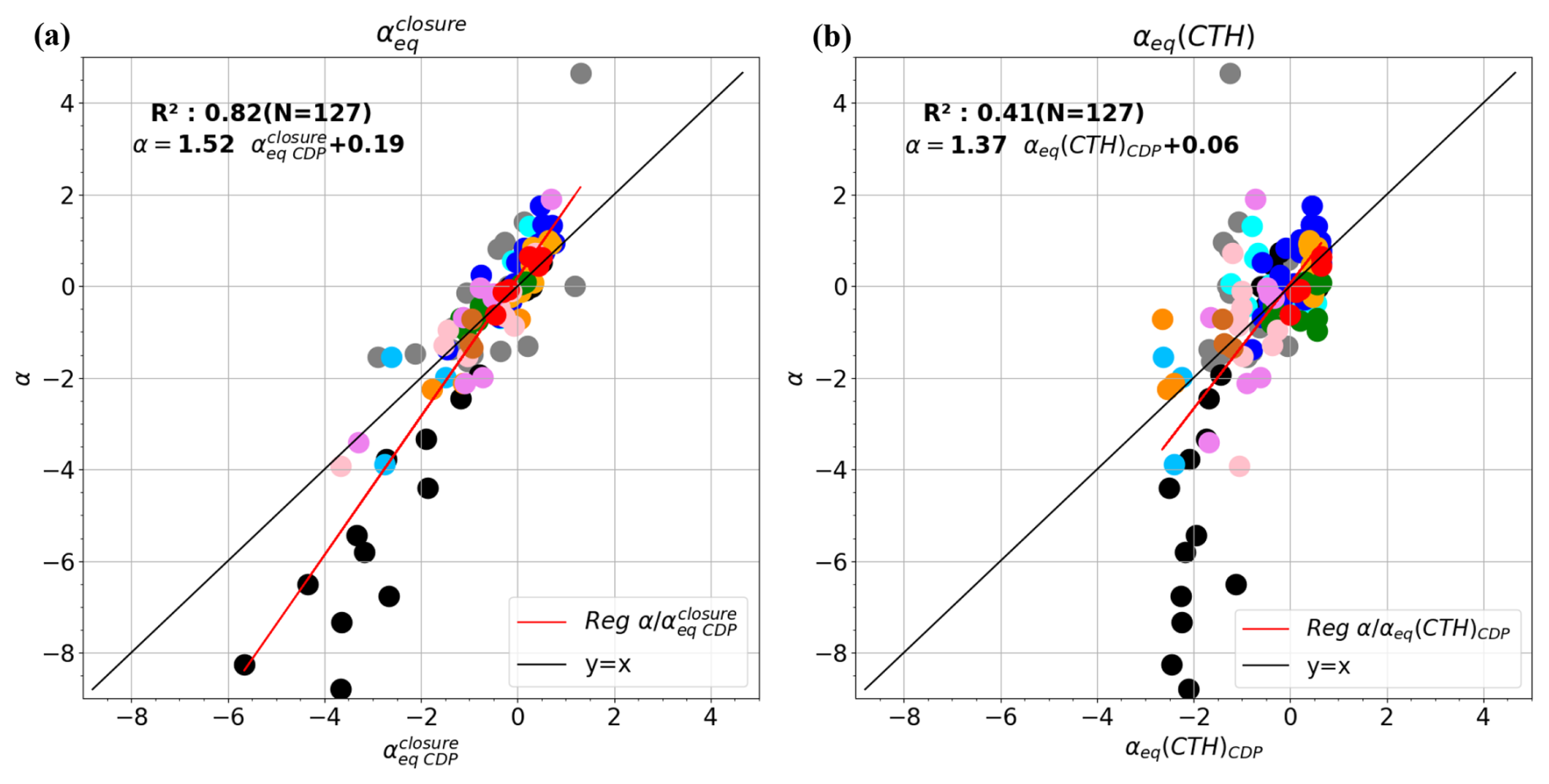
Figure 7 Adiabaticity α as a function of the equivalent adiabaticity (a) from closure issued from the CDP measurements (b) based on the parameterization as a function of the CTH from the CDP using the values retrieved in the previous section for H₀ and L. Each IOP is indicated by a specific colour from IOP 2a to IOP 15 (see legend in Fig. 4).

Comparisons of α with ${\mathit{\alpha }}_{\mathrm{eqCDP}}^{\mathrm{closure}}$ (Eq. 6) and α_eq (CTH)_CDP from the new parameterization are reported in Fig. 7 for the 127 selected profiles in fog. As expected, the absolute values of α are generally larger than those of ${\mathit{\alpha }}_{\mathrm{eqCDP}}^{\mathrm{closure}}$ and α_eq(CTH)_CDP, as attested by the slope of linear regression of 1.52 (Fig. 7a) and 1.37 (Fig. 7b), respectively. Removing the diluted region at fog top for well-mixed fog increases α values. However only a few samples over the 32 profiles identified as increasing with height are significantly impacted, and the comparison with α calculated over the entire profile leads to very similar results (not shown). Some values of α exceed 1, but the examination of such profiles does not reveal any superadiabatic growth. In fact, these values rather result from the uncertainties of the method, which could be very sensitive to the highest values of LWC below the top or LWC₀ at the bottom (e.g. see profiles 6 and 7 of IOP 6 in Fig. 11). This is particularly the case for the first profile of IOP 2a (in grey), where high values of LWC > 0.1 g m⁻³ at 20 m height while condensation at the surface has not yet taken place lead to an α as high as 4.66 as depicted in Fig. C1c. In contrast, given that CTH only reaches 30 m, the parameterization leads to a negative value of α_eq(CTH)_CDP (Fig. 7b). Indeed, as a general trend, the parameterization generates too much negative adiabaticity values due to low values of CTH, ​​while ${\mathit{\alpha }}_{\mathrm{eqCDP}}^{\mathrm{closure}}$ values are positive, in agreement with α. In contrast for thinnest layers, α_eq(CTH)_CDP remained larger than −3, which is clearly overestimated compared to α and ${\mathit{\alpha }}_{\mathrm{eqCDP}}^{\mathrm{closure}}$. Fitting the CDP data produces higher negative values for such reverse LWC profiles. Appendix C1a illustrates the corresponding profile for one of the lowest values ($\mathit{\alpha }=-\mathrm{8.3}$) obtained during IOP 2b, which appears to be realistic given the linear regression on the vertical profile of LWC. Note that for such thin fog layer of 10 m height, the LWP is only 0.7 g m⁻² although LWC₀ reaches 0.1 g m⁻³. Therefore ${\mathit{\alpha }}_{\mathrm{eq}}^{\mathrm{closure}}$ appears to be a better predictor of fog adiabaticity, with an R² value of 0.82, since the parameterization taking only CTH into account does not allow the retrieval of positive adiabaticity values of optically thin fogs and overestimates minimum values of thinnest fogs, leading to an R² value of 0.41.

Reverse LWC profiles for thin fogs were frequently observed during the experiment and are mainly associated with stable atmospheric conditions resulting from radiative cooling established before the fog formation phase. As a next step, the evolution of vertical profiles during the fog life cycle is now studied in more detail to determine to what extent LWC profiles correlate with temperature profiles and how they both evolve during the thin-to-thick transition, when it exists, towards the adiabatic shapes of well-mixed fog layers.

4 Evolution of vertical profile properties during the fog life cycle

The analysis is first carried out on an episode that remains optically thin throughout its life cycle as the majority of fog cases sampled during the SOFOG3D campaign (8 out of 12; Table 2). Then, the contrast with fogs that underwent a transition from optically thin-to-thick is investigated with three other case studies. Finally, a generalization of the thermodynamical and microphysical properties over all fog samples of the 12 IOPs is conducted in Sect. 4.3.

4.1 Thin fog event: IOP 13b case study

The radiation fog sampled during IOP 13b occurred during the night of 23–24 February 2020, associated with anticyclonic conditions and clear sky during the day, leading to a significant radiative cooling shortly after sunset, while wind speed remained low during this period (Fig. 8a). The fog appeared in patches around 20:00 UTC and remained intermittent for 2 h before visibility dropped below 1 km for a longer period between 22:00 and 00:00 UTC (Fig. 8a). At this point, radiative cooling stopped and the temperature stabilized at around 2.5 °C until the fog dissipated at 00:18 UTC due to the advection of a 300 m thick stratus cloud at 23:30 UTC, as depicted by radar reflectivity (Fig. 8c). It should be noted that this fog episode is too thin to be detected by radar, with the exception of a few isolated signals between 25 and 50 m height.

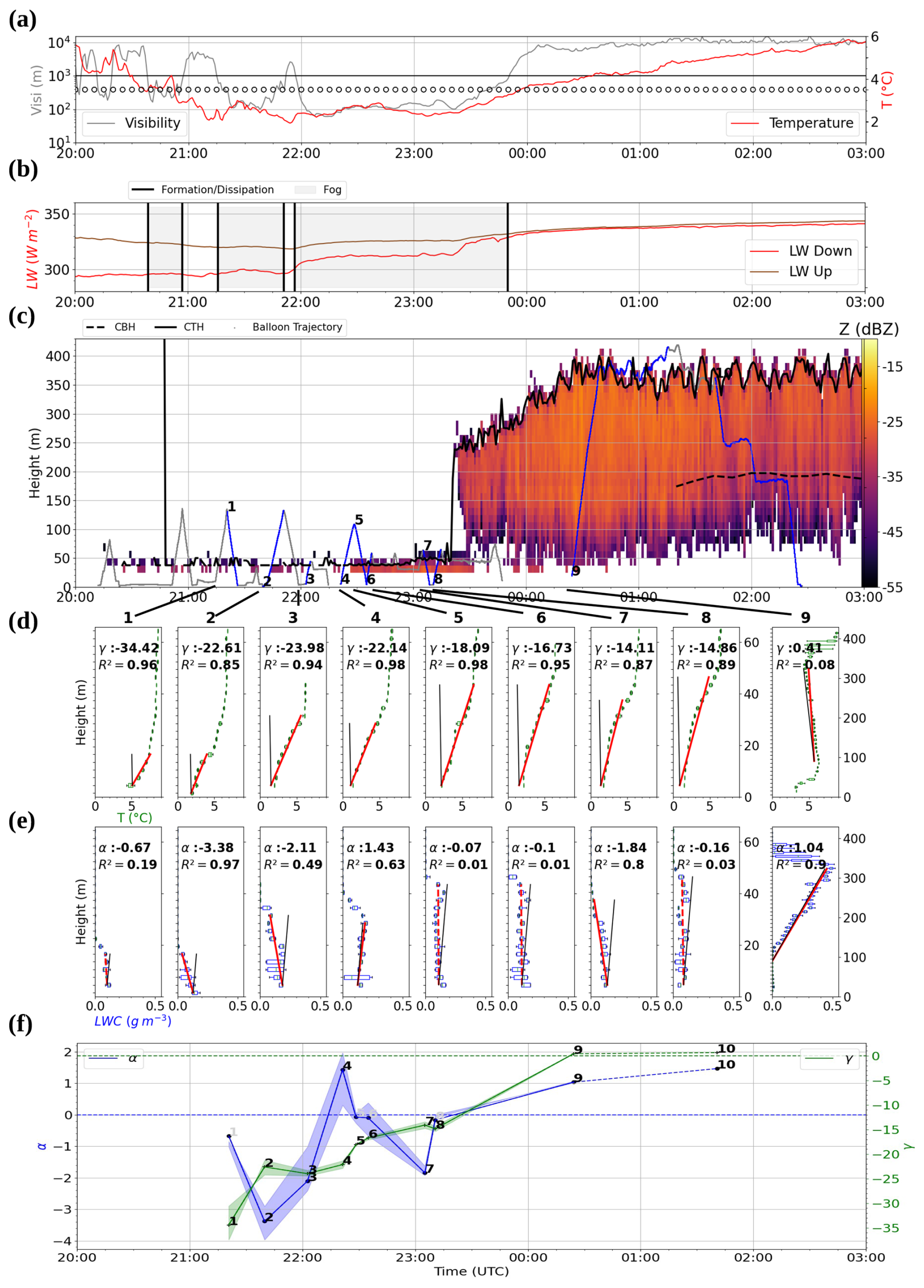
Figure 8 Temporal evolution during IOP 13b at the Charbonnière site of (a) visibility, temperature at 2 m and wind barbs at 10 m above ground level (empty circles, half barbs and full barbs represent wind speeds <2.5, 5 and 10 m s⁻¹, respectively, with the orientation of the barbs giving the wind direction); (b) the upward (brown) and downward (red) longwave radiation. The grey shaded areas delimitate foggy periods; (c) reflectivity and CTH derived from the BASTA cloud radar and CBH (dashed line) from the ceilometer. The trajectory of the tethered balloon is superimposed in grey. Each selected vertical profile is highlighted in blue and labelled by its number. (d) Corresponding vertical profiles of measured temperature, with adiabaticity (red) and adiabatic lapse rate (black). (e) Corresponding vertical profiles of LWC measured by the CDP with adiabaticity (red) and adiabatic (black). (f) Temporal evolution of the adiabaticity for the selected profiles: LWC (blue line) and lapse rate (green line).

The eight profiles performed in the fog layer are displayed in Fig. 8d–e for temperature and LWC, respectively. Despite an increase in the CTH from 20 to 50 m, this fog remains optically thin throughout its life cycle (Fig. 8b). This optical thinness is associated with strong stable vertical profiles of temperature throughout the night, with γ values ranging from −34.4 to −14.1. LWC vertical profiles are characterized by high values of LWC near the ground of around 0.1–0.2 g m⁻³ which tend to decrease with height, particularly profiles 2 and 3 (Fig. 8e), or to remain almost constant. Consequently, α values are also negative throughout the fog life cycle, ranging from −3.4 to −0.07, with the exception of vertical profile 4, which reaches 1.43 due to high variability of LWC near the ground. Figure 8f illustrates the temporal evolution of γ and α during the fog life cycle and clearly shows that both parameters increase progressively with CTH from negative values close to 0 and become positive in the stratus cloud after fog dissipation. Therefore, during a fog episode that remains optically thin throughout its life cycle, stable conditions persist and appear to be associated with a vertical profile of LWC more or less decreasing with height, in contrast to the adiabatic characteristics usually observed in well-developed fogs.

4.2 Fog events with thin-to-thick transition

4.2.1 IOP 14 case study

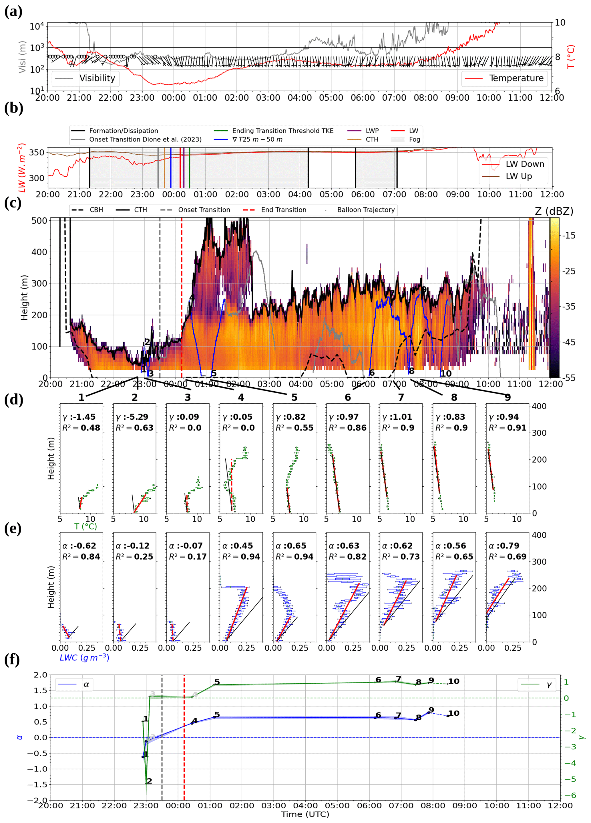
Figure 9 Same as Fig. 8 but for IOP 14. In addition (b) the onset time from Dione et al. (2023) and the different ending times of the thin-to-thick fog transition are indicated by vertical lines, as in Fig. 2; panels (c) and (f) indicate the onset time by a vertical dashed grey line, and the ending time derived from longwave net radiation is indicated by a vertical dashed red line. Visibility in (a) is issued from the Jachère site.

IOP 14 took place on the night of 7–8 March 2020, characterized by a ridge. Shortly after the last residue of the warm front had dissipated, radiative cooling set in over the Charbonnière site, associated with a low wind (Fig. 9a). A low cloud appeared on the reflectivity at around 150 m height at 20:30 UTC (Fig. 9c) and lowered for 40 min before reaching the ground at 21:20 UTC as fog formed. This cloud formation at 150 m height may be explained by the presence of a fence of trees near the Charbonnière site, i.e. in the direction of the wind, as simulated at the SIRTA site by Mazoyer et al. (2017) using large eddy simulations. Due to radiative and advective processes, this fog was classified as a radiative–advective case as in Dione et al. (2023) and not as a fog by stratus lowering due to its rapid descent. The fog layer remained about 100 m thick for 1 h, but the CTH then rapidly lowered as the wind speed aloft dropped, with the wind shifting from SW to SE direction between 22:30 and 23:00 UTC (see Fig. 10d of Dione et al., 2023). The ground temperature then decreased until 23:30 UTC (Fig. 9a) when the fog layer began to thicken again.

The onset of the transition phase is defined at 23:30 UTC following Dione et al. (2023), and the ending times determined from the different parameters are very close, within a 48 min period around 00:12 UTC (Figs. 9b and 2 in Sect. 2.3). In fact, for this case, the advection around 00:30 UTC of a stratus with a base height just above the fog top height contributes to the increase in LWP above the 30 g m⁻² threshold. The CTH derived from the radar also increased sharply above 400 m, but in situ measurements from the tethered balloon attest that it is a distinct cloud layer above the fog. The transition phase duration is therefore short for this case, less than 1 h, and included in the period determined by Dione et al. (2023), which extends to 01:00 UTC. The fog began to dissipate at 04:16 UTC, but visibility remained around 1000–2000 m for 2 h before it dissipated completely at 07:05 UTC, shortly after sunrise, and lifted in stratus cloud that persisted until 10:00 UTC.

The first three vertical profiles with CTH < 80 m reported in Fig. 9d–e were performed during the optically thin phase of the fog event. The first profile reveals low negative values of −0.62 and −1.45 for α and γ, respectively, with a reverse LWC profile which rapidly became almost constant with height for profiles 2 and 3 with α values close to 0. Vertical profiles 4 and 5, which are consecutive descent and ascent after the transition, show contrasting microphysical properties. Profile 4 indicates a continuous increase in LWC with height throughout the fog layer, except at the fog top, consistent with the quasi-adiabatic characteristic. But the α value only reached 0.45, indicating that some dilution has occurred. Vertical profile 5 exhibits a similar trend up to a height of 100 m, but above that, in contrast, the LWC gradually decreased up to the CTH. The temperature profiles show a significant warming between 100 and 200 m height (+2 °C), which explains the evaporation of liquid water in the upper part of the layer. It is likely that this warming is linked to the advection of a stratus above the fog top. In this case, the α value reached 0.65, but this represents only the lower part of the profile. The last vertical profile performed in the fog layer 5 h later also depicts an adiabatic profile, as discussed previously (Fig. 3).

Finally, the three profiles in the stratus following fog dissipation indicate a similar trend with α and γ values between 0.56–0.79 and 0.83–1.01, respectively. Figure 9f illustrates the temporal evolution of α and γ during the fog life cycle, with the thin-to-thick transition indicated by the dashed segment. It appears that α and γ distinctly transition from negative values, when the fog is optically thin, to positive values after the fog development.

4.2.2 IOP 11 case study

IOP 11 took place on the night of 8–9 February 2020, characterized by the establishment of a ridge after an inactive cold front had crossed the country during the day. Shortly after sunset, the sky cleared and radiative cooling set in over the Jachère and Charbonnière sites, leading to the formation of a radiative fog at 20:54 UTC at the Charbonnière site (Fig. 10b). This fog persisted until 03:56 UTC, when advection of warm air at the supersite caused the fog to lift into low stratus, which gradually dissipated until 08:30 UTC.

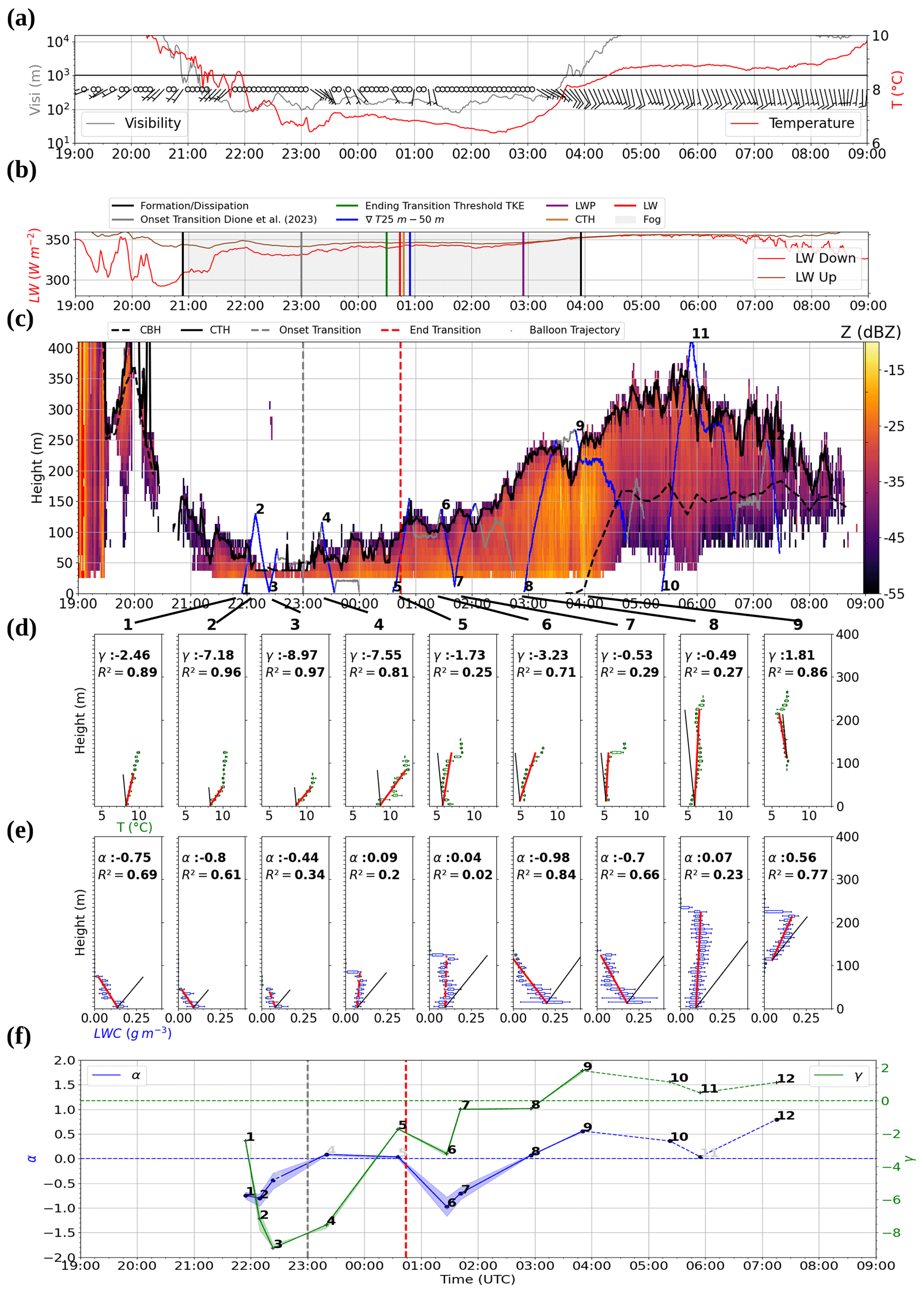
Figure 10 Same legend as Fig. 9 but for IOP 11. Visibility in (a) is issued from the Charbonnière site.

As pointed out in Sect. 2.3, the onset of the transition phase is determined at 23:00 UTC based on Dione et al. (2023), while the end time values are very similar for the different parameters between 00:30 and 00:55 UTC except for LWP, which took 2 h more to exceed the 30 g m⁻² threshold (Fig. A1 in Appendix). Dione et al. (2023) considered that the transition period extended to 02:30 UTC, which is the longest period of their four cases studies.

Of the nine selected vertical profiles reported in Fig. 10d–e, three were performed during the thin phase, two during the transition, three during the thick phase and the last shortly after the fog lifted into stratus. As with IOP 14, the first three vertical profiles during the thin phase with CTH < 80 m present stable lapse rate and reverse LWC profiles with the highest values near the ground. Both α and γ values are negative, but the γ values range from −2.46 and −8.97, which are higher, as for IOP 14, than those obtained during thin fog at IOP 13b, when γ values are systematically lower than −15. Consistently, α values range from −0.44 to −0.8, which are also generally higher than IOP 13b. Note that these higher α and γ values are associated with a thicker fog layer with CTH values from 45 to 75 m compared with the maximum height of 50 m for IOP 13b. It is worth noting that 1 h later, around 23:00 UTC, LWC profile 4 increases slightly with height, in line with the onset of the transition period defined by Dione et al. (2023). The associated temperature profile is still globally stable, but some warming is observed between 65 and 120 m height, which could be explained by the change in wind direction. Below this, the layer between 25 and 65 m has begun to destabilize, possibly reflecting the onset of vertical motions. At the end of the transition phase (profile 5), the entire layer was much colder and unstable. The LWC exhibited a two-layer profile with an adiabatic tendency up to 50 m height and lower values in the upper part.

Surprisingly, reverse LWC trends were observed for profiles 6 and 7 with α<0 even though the thin-to-thick transition had already ended 1 h earlier. In addition, LWC values at the ground reached 0.25 g m⁻³, which are the highest values measured on all IOPs. Note that consistently high radar reflectivities were also observed near the ground (Fig. 10c). The corresponding lapse rates are fairly constant through the layer, contrasting with the stable profiles observed during the thin phase. The LWC profile increases again with a slightly positive α at profile 8 sampled when the fog is 240 m thick, as well as in stratus where α reaches 0.56 with a vertical profile of temperature that has finally destabilized with γ=1.81. The following vertical profiles measured inside the stratus reveal the same microphysical and thermodynamical properties (not shown) as those observed in IOP 14.

Consequently, it is clear from Fig. 10f that the temporal evolution of α and γ during the fog life cycle follows the same trend as for IOP 14, from negative values when the fog is optically thin to positive values after the transition to thick fog, except for the sharp decrease in α for profiles 6 and 7, which disrupts the overall trend, due to sedimentation and collision–coalescence processes as discussed in Sect. 5.

4.2.3 IOP 6 case study

IOP 6 took place during the night of 5–6 January 2020 and was characterized by anticyclonic conditions over France, associated with clear sky and negligible wind. Surface radiative cooling became established on the “supersite” after sunset, and as the south-westerly wind began to blow, ground visibility suddenly dropped by more than 10 km in 10 min (Fig. 11a). This sudden fog formation at 20:37 UTC is associated with the appearance of a 75 m thick liquid water layer on the BASTA reflectivity (Fig. 11c), which was also detected at different heights of the towers surrounding the “supersite” (not shown). Fog formation was spread out over time at the various instrumented sites and was observed earlier and later for the sites located to the southwest and northeast of the domain, respectively (not shown). This suggests that a mesoscale advection coming from the west with moist maritime characteristics favoured the formation of fog in addition to radiative cooling near the ground. Therefore, we rather classify this episode as radiative–advective fog, although Dione et al. (2023) estimated that the formation was mainly driven by radiative cooling at the surface.

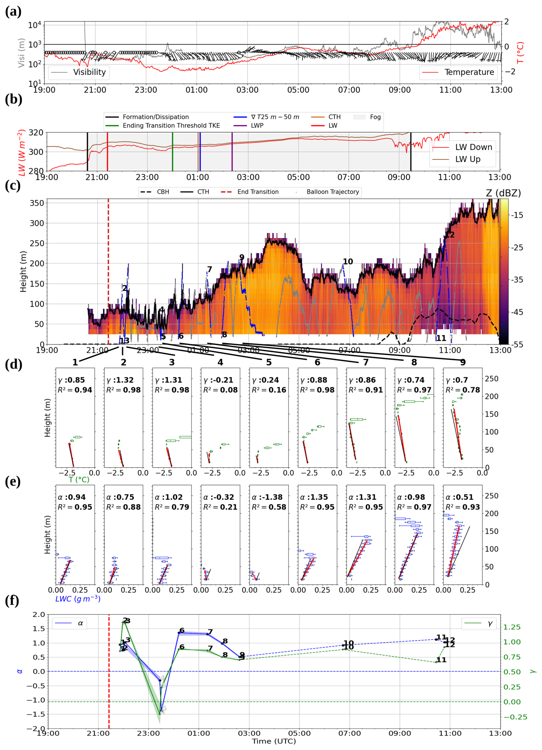
Figure 11 Same legend as Fig. 9 but for IOP 6. Visibility in (a) is issued from the Jachère site.

As discussed in Sect. 2.3, the transition from thin-to-thick fog ended very rapidly (50 min) after fog formation based on LW flux measurements. However, the vertical development of the fog layer was temporarily stopped when the wind direction shifted from southwest to southeast, and it took around 2.5 h for the fog to deepen again around midnight. Consequently, the other parameters indicate a transition ending much later between 00:00 for TKE and 02:30 UTC for LWP, in agreement with Dione et al. (2023), who estimated that the period lasted 2 h from midnight. Finally, the fog dissipated completely at 09:28 UTC, around 1.5 h after sunrise, as it lifted into a deep stratus that persisted throughout the day until it lowered and formed fog again around 16:00 UTC.

Among the 27 vertical profiles validated during IOP 6, 9 representative profiles selected between 21:52 and 03:00 UTC are reported in Fig. 11 to illustrate the evolution of the microphysical and thermodynamical properties during the fog development period. In addition, the α and γ values for the last three profiles when the fog remained adiabatic, despite the decrease in thickness of around 100 m and the rise in stratus (profiles 10 to 12 from 06:00 to 11:00 UTC), are also indicated in Fig. 11f.

As a result, they all show quasi-adiabatic characteristics with positive values of α and γ, except during the period where development is stopped from 22:30 to 00:00 UTC. This confirms that IOP 6 became optically thick very early as indicated by LW measurements. Note that for this case, Dione et al. (2023) classified the period from 20:40 to 00:00 UTC as stable, considering that the transition period started at midnight, as they observed that α_eq (CTH) values remained negative with MWR LWP values <10 g m⁻². In contrast, the first three profiles in Fig. 11d–e show a clear increase in LWC with height associated with the quasi-adiabatic lapse rate. This suggests that other thresholds characterizing the transition with remote sensing measurements should be defined to better detect the transition when the fog life cycle is perturbed by non-local processes.

During the period corresponding to the wind rotation, the CTH dropped from 80 to 30 m in height, and large variability appears in the LWC vertical profiles. The α values decrease and become negative, although the vertical profiles do not reveal decreasing values with maximum values near the ground but rather a constant LWC with height as seen in profile 4, except for the minimum values of $\mathit{\alpha }=-\mathrm{1.38}$ when the fog is at its thinnest (profile 5). During this period, the lapse rate decreased and remained almost neutral (γ≈0) but did not reach low negative values as in previous cases. It is likely that the layer could not return to thermally stable conditions because the time period is too short to allow coupling with the surface, despite the ground temperature losing 1 °C. From midnight, fog thickness increased again. In the same way, the LWC increased with height, and the α values were positive and ranged between 0.51 and 1.35 until the end of the episode, including in the stratus that followed dissipation (Fig. 11f, dotted blue line). As a result, the corresponding temperature profiles are very close to the moist adiabatic lapse rate with γ between 0.7 and 0.88.

This event therefore corroborates the fact that the profiles sampled after the thin-to-thick transition exhibit quasi-adiabatic characteristics with positive values of both α and γ, except when dynamic conditions interrupt vertical development and lead to a significant reduction in fog thickness.

4.3 Correlation between the microphysical and thermodynamical properties

The four case studies presented above have revealed a similar temporal evolution of the vertical profiles of microphysical and thermodynamical properties with contrasting patterns before and after the transition from optically thin-to-thick fog. Values of α and γ of the 140 validated profiles of the campaign are reported in Fig. 12a with empty, full circles, and diamonds, for thin and thick fogs and stratus, respectively, to highlight the contrast between the different phases.

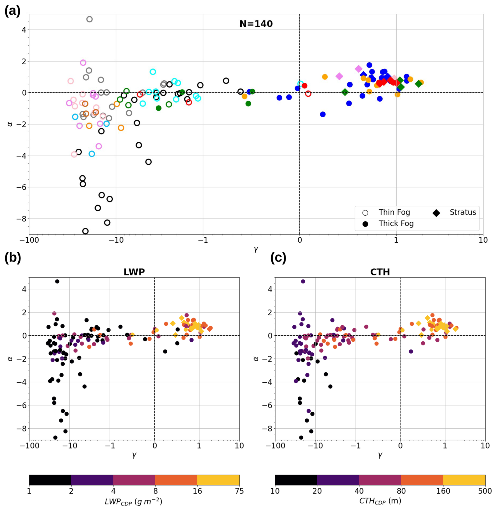
Figure 12 Adiabaticity parameter α as a function of γ in logarithmic scale, over the 12 IOPs: (a) colours of IOPs as in Fig. 4, with open, filled circles, and diamonds for thin and thick fog and stratus, respectively; (b) colour based on LWP values derived from the CDP measurements; and (c) colour based on CTH values derived from the CDP measurements.

A large majority of profiles performed during the thin phase are located in the lower left part of the graph, corresponding to negative γ and α values, while those performed in thick fog are located in the upper right part corresponding to positive or near-zero γ and α values. This trend is particularly marked for the lapse rate. For instance, $\mathit{\gamma }<-\mathrm{0.5}$ for all the profiles performed in thin fog except profile 3 of IOP 14. Similarly, $\mathit{\gamma }>-\mathrm{0.5}$ for all the profiles in thick fog except the two specific reverse LWC profiles of IOP 11. LWC profiles are a bit more scattered, but α<0 for 74 % of the thin cases and α>0 for 75 % of the thick ones. The lowest α values, between −5 and −8, correspond to very stable conditions with $\mathit{\gamma }<-\mathrm{10}$. These profiles performed during IOP 2b are associated with the lowest CTH values <10 m (Fig. 12c) as well as with very low LWP values <2 g m⁻² (Fig. 12b). In contrast, optically thick fogs and stratus by fog lifting are associated with the highest values of LWP and CTH, as illustrated previously by IOP 6c, 13b and 14. In between, intermediate samples of γ ranging between −10 and 0 are associated with intermediate values of α around 0. These profiles are associated with CTH values reaching 50 m but not necessarily with significantly higher LWP values.

An interesting difference when comparing the thin phase of these fogs concerns the range of α and γ. For fogs that remained optically thin during their life cycle, γ ranges from −30 to −15 on average and α from −4 to 0. On the other hand, for those that underwent a transition to thick fog, γ ranges from −10 to 0 and α fluctuates around $-\mathrm{1.5}/-\mathrm{1}$. This would suggest that fogs that remained thin are associated with much stable conditions and stronger reverse LWC profiles. But there are only three thick cases sampled before the transition, and more data are needed to confirm this result.

In conclusion, the analysis of the 140 profiles sampled during the experiment reveals significant differences between thin and thick fogs, with adiabaticity parameters being much lower for thin fogs (α<0, $\mathit{\gamma }<-\mathrm{0.5}$) than for the thick ones and stratus (α>0, $\mathit{\gamma }>-\mathrm{0.5}$). This confirms the temporal evolution from reverse LWC profile and stable conditions during the thin phase to quasi-adiabatic features after the transition as depicted by the three deepest IOPs.

5 Discussion

The CDP data collected below the tethered balloon have revealed a reverse trend of the LWC profile (LWC being maximal at the ground and decreasing with altitude) when stable temperature conditions exist during the optically thin phase of fogs. Oliver et al. (1978) obtained similar shapes of LWC profiles in advective–radiative fog by using a second-order closure model of turbulence. But in their simulation, the fog forms in an unstable mixed layer initiated by the advection of a stable boundary layer over a region with warmer surface temperature. Toledo et al. (2021) mentioned that such a shape should exist to explain their observations of ${\mathit{\alpha }}_{\mathrm{eq}}^{\mathrm{closure}}<\mathrm{0}$. By using cloud radar reflectivity measurements, Wærsted et al. (2017) also retrieved higher LWC values near the ground for a thin fog event. But to our knowledge, only two cases of LWC vertical profiles decreasing with height have been reported in the literature. Okita (1962) measured one profile in a very thin layer <20 m just after the fog formation. More recently, one of the two profiles through the radiative fog sampled during IOP 1 of the LANFEX experiment in Boutle et al. (2018) also presented higher values at the surface, with CTH <40 m and LWP <15 g m⁻². Measurements presented here then suggest that such features are ubiquitous in optically thin fogs. Because such cases also correspond to a geometrically thin fog layer (typically from 10 to 50 m height), the LWP is very low (typically a few g m⁻²), and these properties can hardly be captured by current remote sensing instruments (first available gate of the cloud radar from 25 to 37.5 m height).

We therefore use these in situ data to compute adiabaticity parameters α and γ using linear regressions in order to best fit the vertical profiles of LWC and temperature, respectively. This method allows the removal of the impact of the mixing at fog top, and it is not very sensitive to significant gradients between two consecutive altitude ranges. As a result, it provides valuable information to investigate departure of the general trend of the profile from the adiabatic model and to document the evolution during the fog life cycle, highlighting the contrast between optically thin and thick fogs. However, these calculations must be interpreted with great caution when the fog layer is thin or very thin (lower than 10 m), because it may lead to very low or very high values of α and γ when LWC and temperature gradients are calculated on a reduced number of data. Figure C1a in the Appendix illustrates that the methods work perfectly for a sharp decrease in LWC at an altitude of 10 m, resulting in a very low value of α at −8.26. But Fig. C1c–d report measurements from the first profile sampled during IOP 2a, which exhibit the highest α value (4.66) with one of the lowest γ values (−20). This particular profile was performed at the very beginning of fog formation, when condensation first occurred at a height of around 20 m before the surface, thus distorting the slope calculation and giving a misleading result. This is also the case for profile 4 of IOP 13, where slightly high values of LWC at 30 m height combined with some low values at 10 m height lead to an α value of 1.4, whereas the profile appears to be fairly constant with altitude. Thick fogs are also subject to crude approximation when profiles are not monotonic, such as LWC profile 5 of IOP 11 and IOP 14. In such cases α values obviously cannot represent the shape of the profiles.

Nevertheless, despite such uncertainty, this analysis has shown that these reverse LWC profiles sampled during the thin phase evolve towards quasi-adiabatic features with increasing LWC values with altitude and a neutral to slightly unstable temperature lapse rate, when the transition to optically thick fog occurs. The three deepest episodes presented previously provide convincing elements that highlight such evolution of the vertical profiles during the fog life cycle. The number of sampled profiles, however, is limited, and these fog life cycles were perturbed by non-local processes such as low cloud advection or changes in wind direction, which complicate the interpretation of the observations. On the whole, however, the 140 profiles sampled during the experiment provide a robust assessment of this finding.

To determine the transition phase duration independently of the tethered balloon measurements, we used the onset time determined by Dione et al. (2023) and defined five thresholds for LW flux, TKE, vertical temperature gradient, CTH and LWP for the ending time. Optical depth, which enables one to discriminate between optically thin and thick fogs, was also analysed using the CDP, but the non-continuous measurements did not allow the accurate estimation of the end of the transition phase. We found that the threshold values of 5 for optical depth and 30 g m⁻² for LWP proposed by Wærsted et al. (2017) are too high for our cases and that values of 2 and 15 g m⁻², respectively, are more suited. Dione et al. (2023) also found that the adiabaticity from closure α_eq (CTH) exceeds 0.5 when LWP >20 g m⁻². In fact, in general, the fogs sampled at the Charbonnière site during SOFOG3D have lower LWP values than previous studies at SIRTA (Wærsted et al., 2017; Toledo et al., 2021), but they are similar to IOP 1 of LANFEX (Boutle et al., 2018). Note that LWP measurements at Agen in the Garonne valley during SOFOG3D were much larger, confirming that site characteristics determine fog layer properties. Note also that while the 30 g m⁻² LWP threshold is too high for our dataset, the CTH threshold is adequate. This is confirmed by the new parameterization of ${\mathit{\alpha }}_{\mathrm{eqCDP}}^{\mathrm{closure}}$ (CTH), which exceeds 0.5 when CTH reaches 110 m.

Transition ending time estimates from these different parameters are in agreement during IOPs 11 and 14, during which there was a clear thin-to-thick transition (uncertainty periods of 25 min, and 48 min, respectively), but they are more dispersed during IOPs 9a and 6c (uncertainty periods of 2 h and 29 min and 4 h and 5 min, respectively) since the fog became optically thick immediately after its formation or shortly after, respectively. It is worth noting that the evolution of the LWC profiles is consistent with these transition period estimations, with reverse profiles before the onset of the transition evolving towards an increase in LWC with altitude after the end of the transition. With respect to IOP 6c, the LWC profiles provide a finer-scale understanding of the fog evolution, confirming that the layer is already thick very shortly after the fog onset and becomes temporarily thin as the wind direction changes. Recently, Dione et al. (2023) proposed to additionally use the parameterization α_eq (CTH) to better discriminate the different phases of the fog life cycle (stable, transition, adiabatic and dissipation). The resulting durations of the transition from stable to adiabatic phase for IOP 11, 14 and 6 are 3.5, 1.5 and 2 h, respectively (their Table 2). The durations derived from our analysis are shorter, about 1.5–2 h, and less than 1 h, for IOP 11 and 14, respectively. These discrepancies mainly arise from their criteria that determine the end of the transition phase, namely when α_eq (CTH) >0.5 for IOP 11, but this remained unclear for IOP 14. For IOP 6, the beginning of the transition provided by Dione et al. (2023) is delayed and corresponds to the second vertical development of the fog layer. Then, time series reported in Dione et al. (2023) indicate a promising evolution of α_eq (CTH) during the fog life cycle with respect to periods of thin and thick fog, but further case studies are needed to better define the key parameter values for characterizing the transition.

We have shown that large differences exist between LWC₀ values derived from the CDP and from the visibility by the parameterization of Gultepe et al. (2006) that contribute to the uncertainty in the calculation of ${\mathit{\alpha }}_{\mathrm{eq}}^{\mathrm{closure}}$. Figure 13 reveals that LWC₀ values from CDP data are higher as α decreases for thin fogs, although there is a large dispersion, while there is a significant reduction of LWC₀ values for α>0. This suggests that LWC near the ground decreases after the transition, as the LWC profile is changing from reverse to increasing with height. This is consistent with observations of Mazoyer et al. (2022) that reveal a decrease in the LWC measured near the ground during the mature phase of fogs, resulting from the evaporation due to surface warming induced by infrared radiation emitted by the fog itself.

Figure 13 LWC₀ as a function of the adiabaticity α for the 12 IOPs with the same symbols as Figs. 4 and 12.

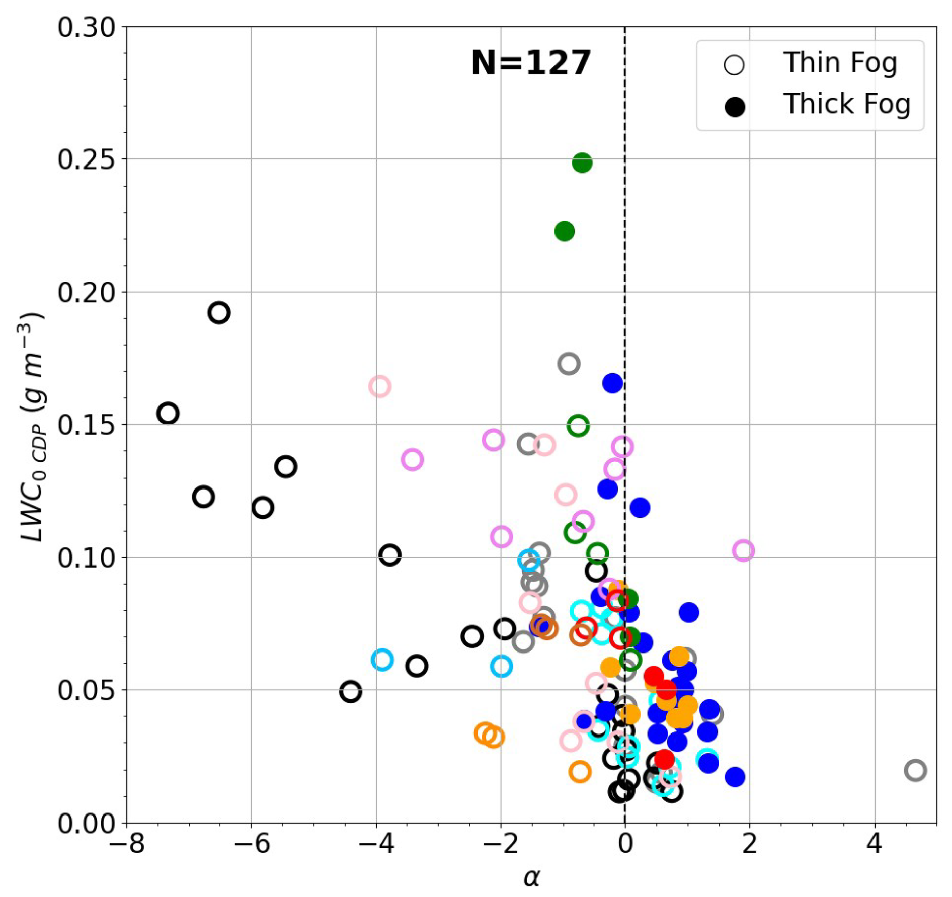
Profiles sampled after the transition exhibit a continuous increase in the LWC with height, but with a large variability of the adiabaticity, profiles 6, 7 and 8 of IOP 6 are very close to the adiabatic trend, whereas profile 4 of IOP 14 and profile 8 of IOP 11 are much more diluted throughout the fog layer. We have seen that ${\mathit{\alpha }}_{\mathrm{eqCDP}}^{\mathrm{closure}}$ values for the few thick profiles with CTH > 150 m sampled with the CDP fluctuate around 0.4, which is below the convergence value ≈0.6 reported for fog conditions in Toledo et al. (2021) and Dione et al. (2023). During SOFOG3D, 13 profiles were performed in stratus cloud. They reveal that the adiabaticity is also highly variable, with profile 9 of IOP 13b adiabatic and others very diluted such as profile 8 of IOP 14 or profile 9 of IOP 11. The mean ${\mathit{\alpha }}_{\mathrm{eqCDP}}^{\mathrm{closure}}$ value reaches 0.61 with first and third quartiles of 0.48 and 0.67, respectively, and the mean α value reaches 0.76 with first and third quartiles of 0.56 and 1.01, respectively. These statistics are in agreement with the typical adiabaticity of 0.7 observed in stratocumulus clouds from airborne measurements (Brenguier et al., 2011; Cermak and Bendix, 2011; Braun et al., 2018). This confirms that these lower adiabaticity values derived from CDP measurements result from the actual properties of the sampled fogs. Other case studies are obviously necessary to assess whether this is a general trend and to better understand the processes that explain such characteristics.

As pointed out previously, the three LWC profiles sampled after the transition during IOP 11 depict a very unexpected trend. Profile 5 presents a two-layer structure with adiabatic increase until 50 m height and reduced values above. Such a shape has already been observed in a fog formed by stratus lowering (Fathalli et al., 2022), but it remains difficult to explain. The wind and temperature profiles reported in Dione et al. (2023) (their Fig. 8d) indicate wind speed shear and strong cooling after 23:00 UTC below 200 m height, suggesting that differential advection could explain this two-layer structure. Surprisingly reverse LWC trends are observed for profiles 6 and 7 sampled less than 1 h later with the highest LWC₀ values measured near the ground (0.25 g m⁻³). Interestingly, these two LWC₀ values come out of all the samples in Figs. 6, 12a and 13. Given that these profiles were sampled 1.5 h after the transition when the fog layer was well developed, with LWP >10 g m⁻² and CTH >120 m and the lapse rate slightly unstable: it is very unlikely that these reverse profiles result from condensation at the surface due to radiative cooling, as observed during the thin phase of radiation fogs.

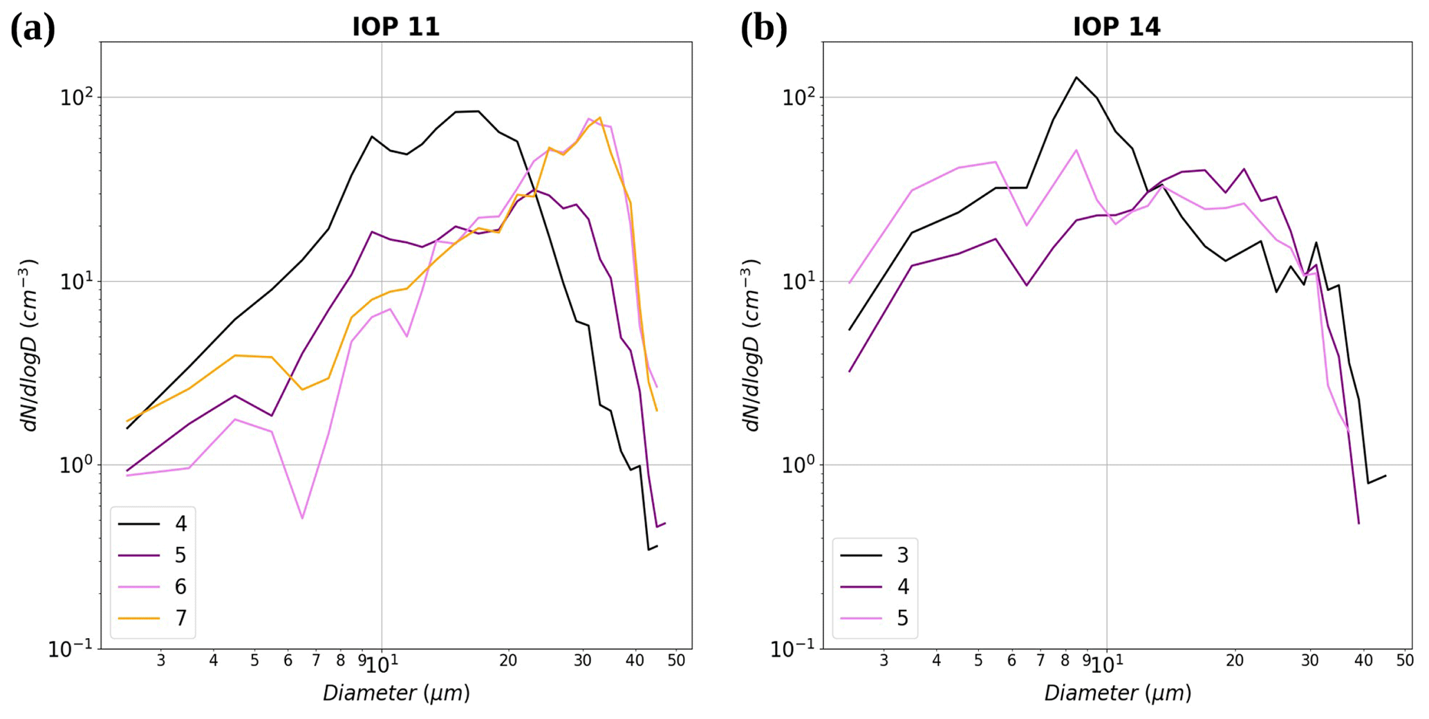
Figure 14 Droplet number size distributions measured by CDP in the 15 m thick layer above the surface for profiles (a) 4 to 7 from IOP 11 and (b) 3 to 5 from IOP 14.

Indeed, these high values of LWC₀ result from the existence of a mode of large droplets as attested by Fig. 14a, which shows the evolution of the droplet number size distributions (DSDs) measured by the CDP at the surface during IOP 11. Initially centred around 15–20 µm (profile 4, black line), the DSD broadens and shifts towards larger sizes during the transition (profile 5, purple line). Finally, for profiles 6 and 7, the DSDs near the ground are very similar with modes as large as 35 µm. In contrast, for IOP 14 (Fig. 14b), the DSD before the transition exhibits a mode below 10 µm, which is further shifted to about 20 µm. Note that droplets as large as 30 µm also exist but at a much lower concentration. DSDs with such modes of large droplets have been observed in many experiments, such as those reported in Wendish et al. (1998), Gultepe et al. (2009), Niu et al. (2011), Formenti et al. (2019), Mazoyer et al. (2022), and Wagh et al. (2023). Usually, they are mainly observed in bimodal DSD and are attributed to a mass transfer from the smaller droplets into the larger ones through collision–coalescence or Ostwald ripening processes and droplet removal through sedimentation. It is remarkable here that the DSDs of profiles 6 and 7 of IOP 11 have a single mode and are very narrow with a high concentration of large droplets. In addition, vertical profiles reveal that LWC has decreased in the upper part of the fog layer, also contributing to the reversal of the LWC trend with height. It is therefore likely that collision–coalescence and sedimentation processes actively contributed to produce such features by redistributing the liquid water through the fog layer from the top to the ground. A more detailed analysis of the evolution of the vertical profile of the microphysical properties is currently being conducted to confirm this hypothesis and will be presented in a related article to be submitted soon.

6 Summary and conclusions

The aim of this study was to document vertical profiles of microphysical and thermodynamic properties in fog layers from in situ measurements collected under a tethered balloon during the SOFOG3D field campaign. Droplet size distributions recorded by an adapted CDP provide 140 vertical profiles of LWC, which allow an exhaustive analysis of eight thin fogs (thickness <50 m) and four developed layers, including three episodes exceeding 200 m in thickness. These data reveal that reverse trends of LWC profiles (LWC being maximal at the ground and decreasing with altitude) are ubiquitous in optically thin fogs, while quasi-adiabatic features with LWC values increasing with altitude are mainly observed in well-mixed optically thick fogs. We used remote sensing instruments (microwave radiometer and Doppler cloud radar) and surface measurements to determine the thin-to-thick transition ending time, based on five thresholds for LW flux, TKE, vertical temperature gradient, fog top height and LWP, enabling us to assess an associated interval of duration. We also used CDP data to compute optical depth on vertical profiles to provide independent measures to discriminate optically thin and thick fog periods. We found that a LWP threshold value of 15 g m⁻² and an optical depth threshold value of 2 are more suited for the four thick fogs sampled at the Charbonnière site than the values of 30 g m⁻² and 5, respectively, proposed by Wærsted et al. (2017). No tendency is observed between the time interval during which the different thresholds are reached and the duration of the transition period.

The CDP data are used to compute the equivalent fog adiabaticity from closure and to compare to the value defined by Toledo et al. (2021), which is derived from remote sensing instruments, 2 m height visibility and an one-column conceptual model of adiabatic continental fog assuming that LWC linearly increases with height. The comparison shows a large variability resulting from differences between both LWC values at ground level and measurements of LWP, but their evolution as a function of the fog thickness follows the same trend, demonstrating the consistency between both methods. A new parameterization of the equivalent fog adiabaticity as a function of fog thickness was developed, on the basis of CDP observations, extending the previous parameterization for optically thin fogs. In addition, we found large negative values for thin layers, associated with low LWP values, that represent a specificity of the fog layers sampled at the Charbonnière site during the SOFOG3D experiment. In situ data are further used to investigate the actual fog adiabaticity parameters α and γ by using linear regressions to best fit the vertical profiles of LWC and temperature, respectively. We presented an analysis of four episodes that highlights that reverse LWC profiles, when stable temperature conditions exist during the optically thin phase of fogs, evolve towards quasi-adiabatic features with increasing LWC values with altitude and neutral to slightly unstable temperature lapse rate when fog becomes thick. This study reveals that non-local processes, such as low cloud advection or changes in wind direction, perturb the fog life cycle and modulate the thin-to-thick transition. On the whole, however, the 140 profiles sampled during the experiment provide a robust assessment of the vertical profile temporal evolution. We also found that LWC at ground level is higher during the thin phase and significantly decreases as the profile changes from reverse to increasing with height. But this trend could be balanced when collision–coalescence and sedimentation processes redistribute the LWC through the fog layer from the top to the ground.

This study provides new insights into the evolution of LWC profiles during the fog life cycle that would help constrain numerical simulations. Although this analysis is based on 140 vertical profiles, the number of samples collected during the thin-to-thick transition remains limited. More continuous observations are therefore required to examine the triggering factors of this transition and to disentangle the local and non-local processes involved in the fog life cycle. The method developed to evaluate the adiabaticity by fitting the vertical profiles of LWC allows the removal of the impact of mixing at the fog top. However, the results revealed large variability among the different cases, with some profiles highly diluted. More analysis is then needed to explain such a departure from the adiabatic model in well-mixed fogs.

To take a step forward, we are currently conducting a detailed analysis of the vertical profiles of droplet size distribution measurements. Following Mazoyer et al. (2022), the main objective is to investigate the vertical and temporal evolution of the droplet size as a function of the number concentration. The vertical profile dataset is extended with constant-height sections at various altitudes within fog layers, which were performed for TKE measurements. Reflectivity and Doppler velocity along the sight of water drops, measured by the BASTA cloud radar, also provide valuable information on the dynamical and microphysical properties of the fog layer (Vishwakarma et al., 2023; Dione et al., 2023). A scanning unit was deployed around 1 km from the vertical pointing unit of the Charbonnière site, which allowed for the first time a volume sampling of a fog layer. Investigation of these data in synergy with CDP measurements would improve the three-dimensional retrieval of microphysical properties and provide new insights to better understand the key processes driving the microphysical evolution during the fog life cycle.

Appendix A: Determination of the thin-to-thick transition time

A1 IOP 11

As for IOP 14 (Fig. 2), there is consistency in the temporal determination of all the thresholds for the time of the transition phase ending (Fig. A1), which range from 00:30 UTC (TKE, green line) to 00:55 UTC (vertical temperature gradient, blue line), i.e. an amplitude of 25 min (Table 2), the onset time being determined at 23:00 UTC following Dione et al. (2023).

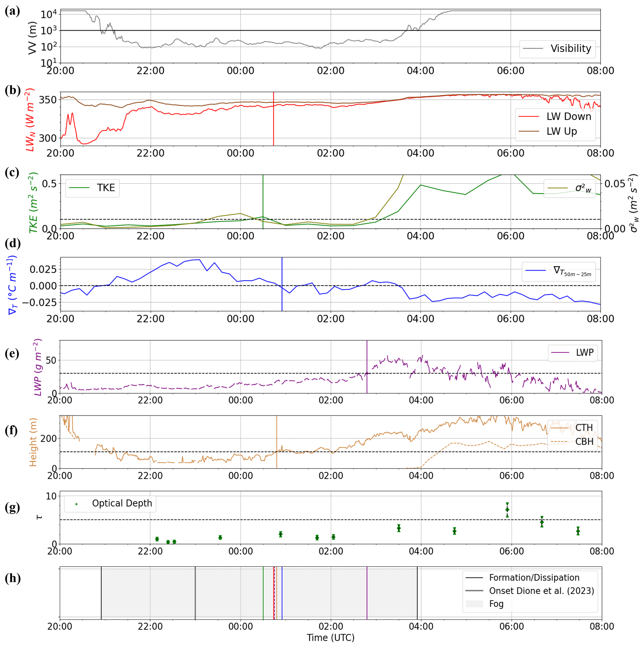
Figure A1 Same legend as Fig. 2 but for IOP 11. Visibility in (a) is issued from the Charbonnière site.

Figure A2 Same legend as Fig. 2 but for IOP 6.

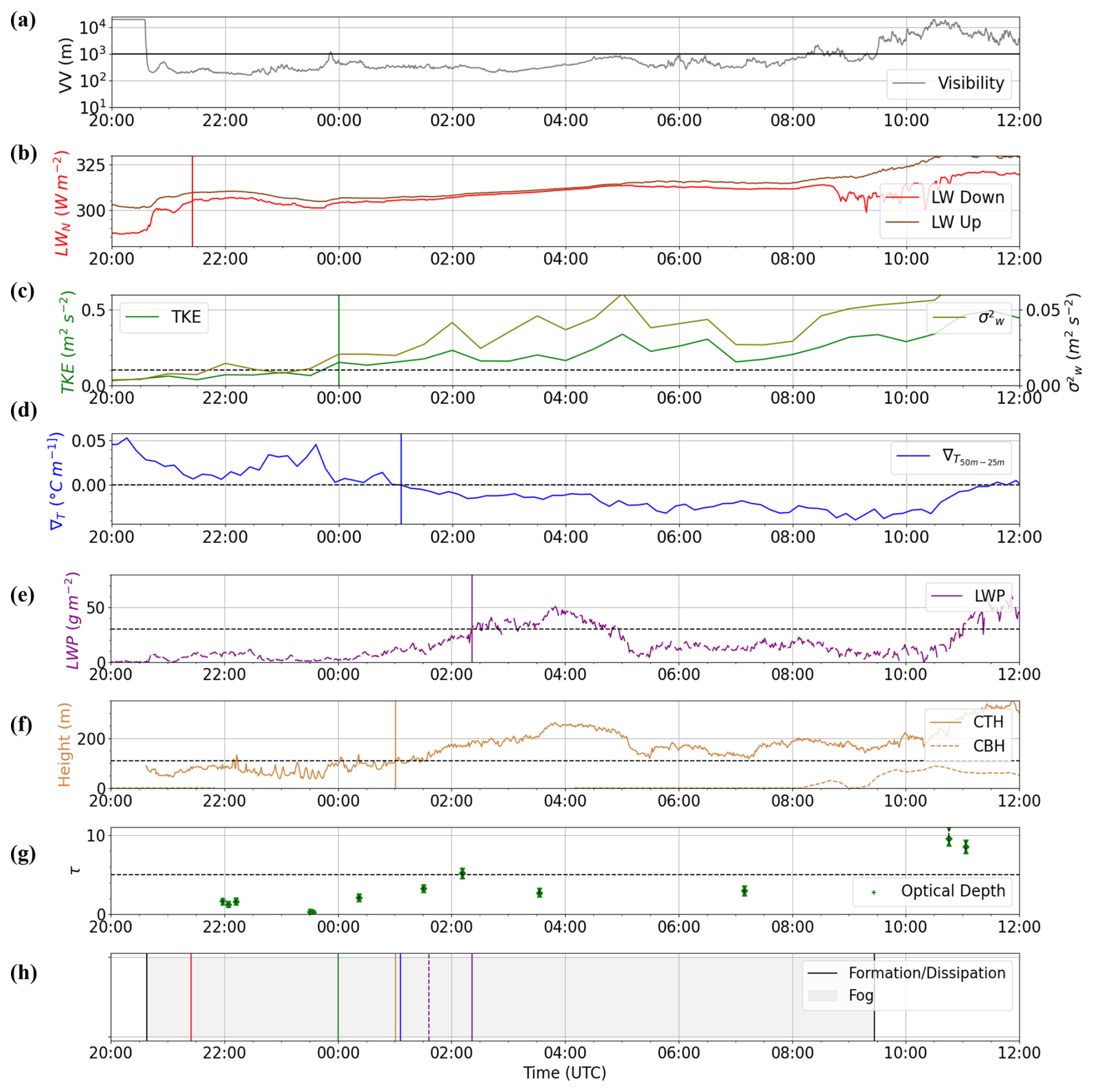
A2 IOP 6

A significant variability is observed in the temporal determination of the transition phase ending between all the thresholds (Fig. A2). Downward longwave radiation strongly increases at the fog formation, leading to a decrease in LW_N, reaching 5 W m⁻² at 21:26 UTC, 49 min after the fog formation at 20:37 UTC (Fig. A2b). At this point, a decrease in vertical temperature gradient is observed, with the fog layer closest to the ground becoming almost neutral and therefore almost reaching the vertical temperature gradient threshold (Fig. A2d). An increase in LWP and CTH is also observed at this time, with the latter close to the 110 m threshold (Fig. A2f). Then, all the variables diverge from their respective threshold, with the exception of LW_N. When the fog deepens vertically at around 00:00 UTC (Fig. 11), TKE exceeds its threshold, while CTH, vertical temperature gradient and LWP thresholds are reached later, between 01:01 and 01:36 UTC. Evolution of the optical depth follows this trend, with values close to 2 shortly after fog formation and up to 6 after the vertical development at around midnight.

Appendix B: Fog equivalent adiabaticity from closure

Figure B1 illustrates the comparison between the values of ${\mathit{\alpha }}_{\mathrm{eq}}^{\mathrm{closure}}$ and LWP as well as CTH, using the measurements retrieved from the HATPRO radiometer and the BASTA radar, respectively. The results are quite similar to those using the CDP measurements (Fig. 6). However, as in Fig. 6, some vertical profiles exhibit superadiabatic behaviour. The two profiles during IOP 2a (in grey) show ${\mathit{\alpha }}_{\mathrm{eq}}^{\mathrm{closure}}$ values greater than 1 due to low LWC₀ values, which are associated with low LWP and CTH values as well, resulting in a strong overestimation of ${\mathit{\alpha }}_{\mathrm{eq}}^{\mathrm{closure}}$. In addition, the superadiabatic vertical profiles during IOP 14 (red) and IOP 11 (green) are associated with a value of CTH just above the detection limit of the BASTA radar.

Figure B1 Same legend as Fig. 6 but using LWP and CTH derived from the HATPRO radiometer and BASTA radar, respectively.

Appendix C: Vertical microphysical properties

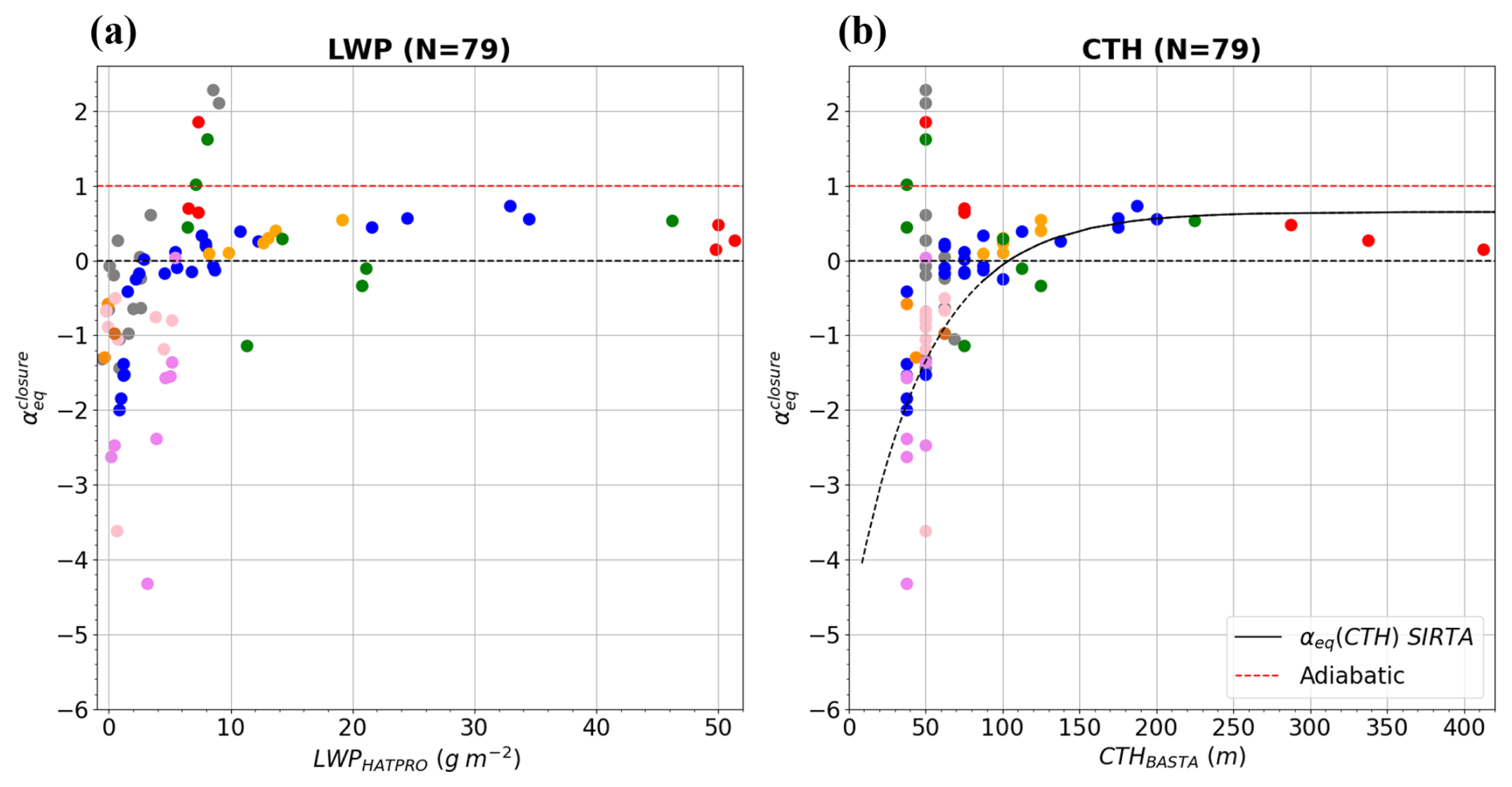
Figure C1a and b show the vertical profiles of temperature and LWC during IOP 2b. This IOP is characterized by three distinct fog periods: between 19:24 and 21:10 UTC, associated with a 130 m thick fog; between 00:02 and 01:36 UTC with a 60 m vertically thick fog; and between 03:31 and 05:13 UTC, associated with a thin fog with a maximum CTH of 30 m. These dissipations may be explained by the presence of temporary medium and low clouds detected by the BASTA radar at around 21:30 and 01:00 UTC, close to 3000 and 1100 m, respectively. The two vertical profiles illustrated in Fig. C1a and b are representative of the last fog episode, characterized by very low values of α and γ. Figure C1c and d show the vertical profiles of temperature and LWC for the first sample during IOP 2a, which reveals a sharp increase in LWC below the fog top, related to condensation occurring at 20 m a.g.l. before the surface.

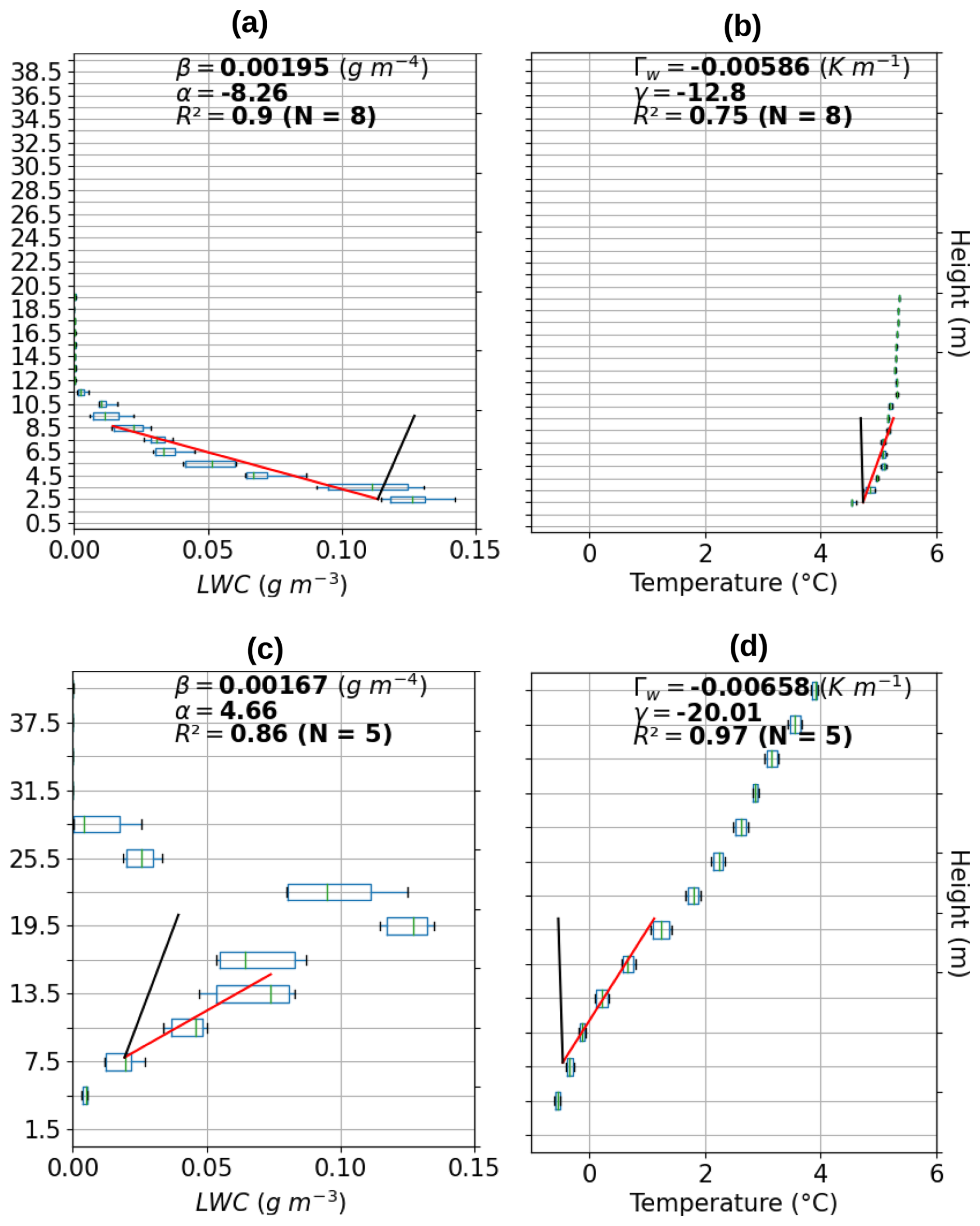
Figure C1 Vertical profile of (a, c) LWC (b, d) temperature during (a, b) the ascent between 03:36 and 03:39 UTC of IOP 2b and (c, d) the ascent between 21:39 and 21:41 UTC of IOP 2a. N corresponds to the number of points used for the linear regression.