Representing improved tropospheric ozone distribution over the Northern Hemisphere by including lightning NO_x emissions in CHIMERE

Estimating nitrogen oxide emissions from lightning (LNO_x) in models is highly uncertain, affecting the accuracy of atmospheric composition and air quality assessments. Still, it is essential to include these emissions in models to increase the realism of representing the gases and aerosols. LNO_x emissions have recently been incorporated into the updated version of the CHIMERE model (v2023r2). In this study, we evaluate the present state of modelling the lightning flashes over the Northern Hemisphere (NH), using a classical scheme based on cloud-top height (CTH) and an updated ice-flux-based scheme (ICEFLUX). We conduct a comprehensive 3D comparison of model outputs, including in situ measurements and satellite data, to rigorously assess the robustness and applicability of these parameterizations. The comparative analysis reveals that the CTH scheme provides a more accurate spatial variability of lightning flashes over lands and tropical oceans. Both parameterizations accurately capture the magnitude of lightning flashes over the tropics, while the ICEFLUX scheme is more effective in representing mid-latitudinal flashes. However, both schemes perform well in capturing the seasonal variation of lightning flashes. The estimated flash frequencies over the NH from the experiments closely align with satellite observations, and the LNO_x emissions fall within the range reported in previous modelling studies. There is an overall increase in ozone (O₃) concentration due to inclusion of LNO_x, which substantially improves the tropospheric O₃ distribution, specifically in the tropical free troposphere. The LNO_x emissions hence critically influence the O₃ burden as well as the hydroxyl radicals, which further impact the atmospheric lifetime of trace gas methane.

1 Introduction

Nitrogen oxides (NO_x), consisting of nitric oxide (NO) and nitrogen dioxide (NO₂), are trace gases that play a key role in atmospheric chemistry, particularly in the formation of tropospheric ozone (O₃) (Finney et al., 2014; Luo et al., 2017; Akimoto and Tanimoto, 2022). NO_x emissions arise from both anthropogenic sources, e.g., fossil fuel combustion; biomass burning; and natural processes, such as lightning and soil-NO_x emissions (Verma et al., 2021; Butler et al., 2020). Among these sources, lightning-induced NO_x (LNO_x) contributes approximately 10 %–15 % to global NO_x emissions, with an even greater contribution (up to 70 %) in the upper troposphere (Maseko et al., 2021; Luhar et al., 2021; Wu et al., 2023). Importantly, LNO_x has a stronger impact on tropospheric O₃ formation compared to surface-based sources, due to the altitude at which LNO_x is injected into the atmosphere and the efficiency of O₃ production in the upper troposphere (Finney et al., 2016a; Luhar et al., 2021). The mean estimated rate of NO_x emissions from lightning is highly uncertain, with recent studies indicating variations ranging between 33–660 mol of NO per flash (Luhar et al., 2021; Bucsela et al., 2019; Murray, 2016; Schumann and Huntrieser, 2007), although Schumann and Huntrieser (2007) suggest a mean value of 250 mol of NO per flash. In spite of this uncertainty, inclusion of these emissions in models is essential to enhance the accuracy and reliability of model projections.

The inclusion of LNO_x in chemistry–transport models has been a research topic for several decades (Kang et al., 2020), with seminal studies (Price and Rind, 1992; Price et al., 1997a; Schumann and Huntrieser, 2007; Allen et al., 2010; Finney et al., 2014) pioneering the quantification of lightning flash rates and their associated NO_x production. These foundational studies laid the groundwork for understanding the contribution of LNO_x to tropospheric chemistry (Allen et al., 2010; Banerjee et al., 2014; Finney et al., 2016a; Kang et al., 2019, 2020). A range of parameterization schemes, including diverse empirical equations, have been developed over decades to quantify lightning flash rates and their spatial distribution (Finney et al., 2014). Despite the significant progress made, challenges remain in accurately quantifying LNO_x emissions, due to uncertainties in characterizing both the spatial and temporal variations in lightning frequency and intensity, the apportionment among cloud-to-ground (CG) and in-cloud (IC) flashes, the rates of NO_x production from lightning discharges, and the vertical distribution and transportation of LNO_x after its generation (Labrador et al., 2005; Schumann and Huntrieser, 2007; Menut et al., 2020a; Wu et al., 2023). Recent studies have focused on improving the representation of lightning in models through various parameterization schemes based on cloud-top height (CTH; Price and Rind, 1992; Price et al., 1997a; Clark et al., 2017), ice flux (ICEFLUX; Finney et al., 2014), convective precipitation, updraught of mass flux (Allen et al., 2000; Allen and Pickering, 2002), and convective available potential energy (CAPE; Choi et al., 2005; Zhao et al., 2009). These approaches aim to better capture the spatial and temporal variability of lightning activity, leading to more accurate estimates of LNO_x emissions.

In this study, we expand on the previous work by implementing the ICEFLUX scheme in the chemistry–transport model CHIMERE and comparing it with the CTH scheme. The CHIMERE model has been developed since 1997 and has been modified on a regular basis for better prediction of trace gases and aerosols (Menut et al., 2020b). The improvement in the natural emissions in the recent version of the model allows for the incorporation of LNO_x emissions (Menut et al., 2024a). The study by Menut et al. (2020a), conducted over a short period of 2 months (July–August 2013), covering Europe and the northern part of Africa, demonstrates changes in tropospheric O₃ and NO_x concentrations resulting from the inclusion of LNO_x emissions in CHIMERE, using the CTH scheme. However, opportunities remain to improve the representation of flash rates in the model. To address this, we have applied the recent ICEFLUX parameterization. The CTH scheme does not incorporate the complex interactions and charge distributions that drive lightning production (Price and Rind, 1992; Finney et al., 2014), nor does it account for detailed microphysical processes, storm dynamics, or the presence of ice particles (Price and Rind, 1992). The improved modelling of cloud ice has facilitated the inclusion of the upward flux of ice crystals (Finney et al., 2014). However, ice flux alone is insufficient to fully capture the complexities of lightning phenomena, as additional factors likely influence the charging process. Therefore, a comparative analysis of the traditional CTH and the updated ICEFLUX schemes is essential to assess their effectiveness in the regional model CHIMERE. We perform a 3D comparison of model outputs with each other and with a simulation devoid of LNO_x. Model outputs are also compared with in situ measurements and satellite data. Furthermore, validating and evaluating these lightning parameterizations across different models (global and mesoscale) are crucial for fully assessing their robustness and applicability, underscoring the significance of this study. Additionally, a thorough evaluation of simulated tropospheric O₃ is also essential to refine model accuracy and deepen our understanding of the role of LNO_x in atmospheric composition.

Lightning-generated NO_x also influences the tropospheric hydroxyl radical (OH) budget, in addition to affecting O₃ concentrations (Murray et al., 2013; Murray, 2016; Mao et al., 2021). The OH radical is primarily formed due to photolysis of O₃ (O(¹D)) at a shorter wavelength (≤ 330 nm) in the presence of water vapour and secondarily through the reaction between hydroperoxyl radical (HO₂) and NO (Lelieveld et al., 2016; Banerjee et al., 2014). As a highly reactive and short-lived oxidant, with a lifetime of just a few seconds, OH is essential to tropospheric chemistry (Lelieveld et al., 2016). However, substantial variability exists among global models, with differences of up to ±30 % in estimating the mean OH burden (Murray et al., 2021). OH further controls the lifetime of many important trace gases, such as methane (CH₄), carbon monoxide (CO), and non-methane volatile organic compounds (NMVOCs) (Akimoto and Tanimoto, 2022; Luhar et al., 2021). For example, the increase in OH burden reduces the lifetime of CH₄ (Reaction 1), a potent greenhouse gas and a major contributor to global warming (Naik et al., 2013; Banerjee et al., 2014; Murray et al., 2021). By improving the parameterization of LNO_x in CHIMERE, this study strengthens our understanding of tropospheric chemistry and the dynamics of trace gases.

$$\begin{array}{}\text{(1)}& {\text{CH}}_{\mathrm{4}}+\text{OH}\to {\text{CH}}_{\mathrm{3}}+{\text{H}}_{\mathrm{2}}\text{O}\end{array}$$

Hence, the specific objectives of the study are (i) to evaluate and improve the modelling of lightning flashes, with the CHIMERE model using the classical CTH and the upgraded ICEFLUX scheme; (ii) to evaluate the effect of LNO_x emissions on tropospheric O₃ and trace gases; and (iii) to evaluate the influence on the OH burden and lifetime of CH₄ quantified against the chemical loss. The detailed methodology is provided in Sect. 2. An analytical evaluation of the simulated results have been carried out and presented in the following sections.

2 Method of study

2.1 CHIMERE model configuration and experimental set-up

In this study, simulations are carried out with the CHIMERE chemistry–transport model (version 2023r2; Menut et al., 2024a) over the domain of the Northern Hemisphere (NH) expanded from 0–90° N, at a horizontal resolution of 100 × 100 km². Here, meteorological fields are forced externally to CHIMERE with a 3-hourly forecast dataset from the European Centre for Medium-Range Weather Forecasts (ECMWF) Integrated Forecasting System (IFS) (https://www.ecmwf.int/en/forecasts/datasets, last access: 16 May 2024). Simulations are done in 20 vertical levels in sigma-pressure coordinates ranging from the surface to 200 hPa for a period of 1 year (January–December 2018) with a spin-up time of 15 d. The MELCHIOR2 scheme is used for the chemical mechanism. The CHIMERE model employs a 10-bin logarithmic sectional size distribution ranging from 0.01 to 40 µm. Fields of chemical concentration are calculated with a time step of a few minutes, using an adaptive time step, to ensure that the Courant–Friedrichs–Lewy (CFL) stability criterion is satisfied (Menut et al., 2021). Boundary and initial conditions are derived from the Copernicus Atmosphere Monitoring Service (CAMS) reanalysis dataset of atmospheric compositions produced by ECMWF, consisting of three-dimensional time-consistent atmospheric composition fields, including aerosols and chemical species (Inness et al., 2019), and from GOCART for dust concentrations (Chin et al., 2002). Biogenic emissions are provided by a reduced online version of the Model of Emissions of Gases and Aerosols from Nature (MEGAN) (version 2.10) (Guenther et al., 2012). Mineral dust and sea-salt emissions are calculated using the schemes of Alfaro and Gomes (2001) and Monahan (1986), respectively. Anthropogenic emissions and fire emissions in the model are incorporated, respectively, from the CAMS Global and CAMS Global Fire Assimilation System (GFAS, https://atmosphere.copernicus.eu/global-fire-emissions, last access: 16 May 2024). The formation of secondary organic aerosols (SOAs) is as described in Pun and Seigneur (2007) and Bessagnet et al. (2008). The aerosol dynamic processes, such as condensation, coagulation, wet and dry deposition, absorption, and scavenging, are incorporated into the model (Menut et al., 2021). The mixing state is considered as internal homogeneous aerosol mixing (Menut et al., 2013). The online calculations for radiation and photolysis are incorporated using the FastJX module (Wild et al., 2000; Mailler et al., 2016). The horizontal and vertical transports are solved with the van Leer (1977) scheme. Boundary layer height and vertical diffusion are calculated by the parameterization proposed by Troen and Mahrt (1986), and deep convective fluxes are estimated using the Tiedtke (1989) scheme. Gaseous and aerosol species undergo dry or wet deposition, and fluxes are calculated using the Wesely (1989) and Zhang et al. (2001) parameterization schemes. With access to anthropogenic and biogenic emissions, CHIMERE simulates 3D concentrations for a range of gaseous and size-resolved particulate species, based on the chosen chemical scheme.

Simulations carried out for this study are (i) not including LNO_x emissions (experiment: noLNOx), (ii) including LNO_x emissions estimated with a parameterization based on cloud-top height (CTH) (experiment: LNOx-CTH), and (iii) including LNO_x emissions estimated with the parameterization based on ice flux (experiment: LNOx-ICEFLUX).

2.2 Parameterization of lightning flash

2.2.1 Cloud-top-height-based parameterization (CTH)

Derived from the theories advanced by Vonnegut (1963) and Williams (1985), Price and Rind (1992) formulated the CTH parameterization, wherein the flash rate is contingent upon the cloud-top height (H_top). The distinct relationships governing flash rates over land and ocean are delineated as follows:

$$\begin{array}{}\text{(1)}& \begin{array}{rl}& F_{\mathrm{l}}=a\times H_{\mathrm{top}}^{\mathrm{4.9}},\\ & F_{\mathrm{o}}=b\times H_{\mathrm{top}}^{\mathrm{1.73}}.\end{array}\end{array}$$

Here, a and b are constants (values are provided in Table 1), and H_top represents the cloud-top height above the ground level in kilometre. Cloud-top height (H_top) and cloud-bottom height (H_bottom) are estimated based on the convection scheme of the model for each time step. F denotes the total flash rate in flash number min⁻¹ 25 km⁻², with subscripts l and o indicating land and ocean, respectively (Menut et al., 2020a). The distinction between land and ocean is employed to incorporate the disparity in updraught velocity over these two surface types. For instances where the cloud depth (H_top−H_bottom) is less than 5 km, the flash number is set to zero. This threshold reflects the physical condition necessary for charge separation and buildup in a storm to generate lightning. The assumption of minimum required cloud depth of 5 km may introduce uncertainty in estimating lightning flashes, as it inherently assumes that every convective cloud with a depth of 5 km corresponds to a thunderstorm (Luhar et al., 2021). It would be worthwhile to investigate the sensitivity of the modelled flash rates to the minimum cloud depth by varying this arbitrary threshold, either increasing or decreasing it. It is noteworthy that Price and Rind (1994) formulated an equation to adapt the above equations to various model resolutions. The scaling factor (C) determined to accommodate the model grid cell size is outlined as follows:

$$\begin{array}{}\text{(2)}& C=\mathrm{0.97241}{e}^{\mathrm{0.048203}\times \mathrm{\Delta }x\times \mathrm{\Delta }y}.\end{array}$$

Here, the product of longitude and latitude resolution, denoted as Δx×Δy, is measured in degrees². This factor typically remains close to 0.97, and its impact on the results is minimal, especially when compared to the uncertainties due to other parameters. These uncertainties are offset by adjustment factors that align the model more closely to observations (Gordillo-Vázquez et al., 2019). In preliminary simulations, we observed a highly overestimated flash rate, estimated based on the formulations by Price and Rind (1992), compared to the measurements from the Lightning Imaging Sensor on the International Space Station (ISS-LIS) for the year 2018, over the land grids, followed by the ocean grids. Considering the overestimation in the modelled flash rate, we have applied factors 0.1 and 0.5, respectively, to constants a and b in Eq. (1) over the land and ocean grids, in experiment LNOx-CTH, to reconcile the modelled lightning flash rate to the satellite observations (Table 1).

Price and Rind (1992)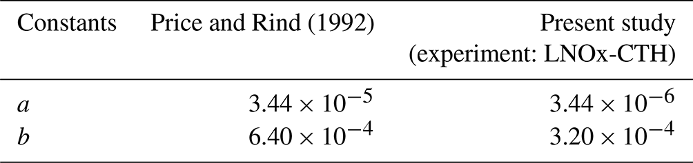

Table 1 Values of constants in Eq. (1).

For each grid cell, the relative fraction of sea (x_sea) is determined using the land–sea mask from the land use database (Menut et al., 2020a). The total flash rate (F_CTH) is then calculated as follows:

$$\begin{array}{}\text{(3)}& F_{\mathrm{CTH}}={\displaystyle \frac{C\times \left(x_{\text{sea}}\times F_{\mathrm{o}}+(\mathrm{1}-x_{\text{sea}})\times F_{\mathrm{l}}\right)}{\mathrm{25}}}.\end{array}$$

2.2.2 Ice-flux-based parameterization (ICEFLUX)

The equations used to estimate the flash rates in the ICEFLUX parameterization are as follows (Finney et al., 2014):

$$\begin{array}{}\text{(4)}& \begin{array}{r}{f}_{\mathrm{l}}=\mathrm{6.58}\times {\mathrm{10}}^{-\mathrm{7}}{\mathit{\varphi }}_{\mathrm{ice}},\\ f_{\mathrm{o}}=\mathrm{9.08}\times {\mathrm{10}}^{-\mathrm{8}}{\mathit{\varphi }}_{\mathrm{ice}}.\end{array}\end{array}$$

Here, f_l and f_o represent the flash rate (flash number m${}_{\mathrm{cell}}^{-\mathrm{2}}$ s⁻¹) over land and ocean, respectively; ϕ_ice denotes the upward ice flux (kg_ice m${}_{\mathrm{cloud}}^{-\mathrm{2}}$ s⁻¹) at 440 hPa and is determined using the following equation:

$$\begin{array}{}\text{(5)}& {\mathit{\varphi }}_{\mathrm{ice}}={\displaystyle \frac{q\times {\mathrm{\Phi }}_{\mathrm{mass}}}{c}}.\end{array}$$

In this context, q represents the specific cloud ice water content at 440 hPa (kg_ice kg${}_{\mathrm{air}}^{-\mathrm{1}}$), Φ_mass denotes the updraught mass flux at 440 hPa (kg_air m${}_{\mathrm{cell}}^{-\mathrm{2}}$ s⁻¹), and c represents the fractional cloud cover at 440 hPa (m_cell² m${}_{\mathrm{cloud}}^{-\mathrm{2}}$). In instances where c is less than 0.01 m${}_{\mathrm{cloud}}^{\mathrm{2}}$ m${}_{\mathrm{cell}}^{-\mathrm{2}}$, upward ice flux is set to zero. Additionally, if no convective cloud top is identified, the flash rate is also set to zero (Finney et al., 2016a). The total flash rate (F_ICEFLUX) is then calculated as follows:

$$\begin{array}{}\text{(6)}& F_{\mathrm{ICEFLUX}}=x_{\text{sea}}\times f_{\mathrm{o}}+(\mathrm{1}-x_{\text{sea}})\times f_{\mathrm{l}}.\end{array}$$

The estimated flash frequency from LNOx-ICEFLUX has been scaled down by a factor of 5 to align with satellite-observed frequencies. Consequently, the evaluation of LNOx-ICEFLUX results has been carried out using these adjusted flash rates.

2.2.3 Distribution of CG and IC lightning flashes

The empirically derived formula used to determine the relative proportion of cloud-to-ground (CG) flashes in a single thunderstorm is initially based on the cold-cloud depth (H_f, from 0 °C to cloud top) (Price and Rind, 1993). In this study H_f (in km) is calculated with the temperature profile in the model, estimating the freezing temperature height or the freezing level. The modelled H_f therefore varies from 6.9 to 7.76 km. The freezing level (0 °C temperature), estimated in the model, varies from 1 to 4.9 km, being the highest in the tropics and decreasing with higher latitudes. The flashes from freezing level to the cloud-top height are considered as in-cloud (IC) flashes, and those from the freezing level to ground are considered as CG flashes. The freezing level acts as a natural boundary between the upper and lower parts of the cloud. Above the freezing level, ice particles contribute to the development of IC lightning, while below it the atmosphere is typically in a liquid state, with the warmer environment aiding in the development of CG lightning (Dwyer and Uman, 2014).

The mean ratio of IC to CG flash rates (β= IC $/$ CG) is estimated as 3.09 from model estimates. β, in this study, is estimated with the empirical equation (Eq. 7) by Price and Rind (1993), which is frequently used in several modelling studies (Luhar et al., 2021; Gordillo-Vázquez et al., 2019). The empirical relationship between β and the cold-cloud depth (H_f) was developed by Price and Rind (1993) based on data collected for 139 individual thunderstorms over the western United States of America (USA) during summer. Several studies support the fact that the parameterization Price and Rind (1993) successfully estimates the distribution of CG and IC flashes in global, as well as in mesoscale, models (Pickering et al., 1998; Fehr et al., 2004). Theoretically, β varies between 1 and 50 for H_f varying between 5.5 and 14 km to prevent unrealistic values. The value of β estimated in our study is comparable to that obtained in recent modelling studies (Luhar et al., 2021; Gordillo-Vázquez et al., 2019). Wu et al. (2023) estimates the values of β as 2.94–3.70 with a lightning nitrogen oxide (LNO_x) emissions model using satellite-observed lightning optical energy. Further, experiments conducted with satellite- and ground-based observations over different parts of the world also produce a β value in the range of 2.64–2.94 (±1.1–1.3) over the USA (Boccippio et al., 2001) and 3–4 over India and China (Ghosh et al., 2023; Ren et al., 2024). β= IC $/$ CG (Eq. 7), obtained in our study, again shows consistency with the above-mentioned results.

$$\begin{array}{}\text{(7)}& \mathit{\beta }=\mathrm{0.021}{H}_{\mathrm{f}}^{\mathrm{4}}-\mathrm{0.648}{H}_{\mathrm{f}}^{\mathrm{3}}+\mathrm{7.49}{H}_{\mathrm{f}}^{\mathrm{2}}-\mathrm{36.54}{H}_{\mathrm{f}}+\mathrm{63.09}\end{array}$$

The relative part of CG in the total (IC + CG) is denoted by p (Eq. 8). The estimated value of p from our study is 0.25, aligning with findings from recent research (Luhar et al., 2021).

$$\begin{array}{}\text{(8)}& p={\displaystyle \frac{\mathrm{1}}{\mathrm{1}+\mathit{\beta }}}\end{array}$$

Hence, the β in our study is not predetermined but is calculated based on the cold-cloud thickness (H_f), which is estimated with the temperature profile in CHIMERE and agrees well with the values estimated theoretically from other model-based studies.

2.3 Estimation of LNO_x emissions

Lightning flash energy estimates span a broad range from 0.35–5 GJ based on length-specific discharge values up to 6.7 GJ considering contributions to the global atmospheric electric circuit (Krider et al., 1968; Uman, 2001; Price et al., 1997a). The NO_x production rate per unit discharge energy also exhibits substantial variation, ranging from 1.1 × 10¹⁶ to 50 × 10¹⁶ molec. J⁻¹ in laboratory experiments (Schumann and Huntrieser, 2007) and 5 × 10¹⁶–15 × 10¹⁶ molec. J⁻¹ in theoretical models (Price et al., 1997a). In this study, we adopt flash energies of 3 GJ for CG flashes and 0.9 GJ for IC flashes, along with a NO production rate of 14.2 × 10¹⁶ molec. NO J⁻¹ (Schumann and Huntrieser, 2007). Using these values, we calculate the NO production in moles per flash as described in Eq. (9), yielding a mean value of 332 mol of NO per flash. This estimation considers CG flashes as 25 % of the total lightning flashes.

$$\begin{array}{}\text{(9)}& \begin{array}{rl}& P(\mathrm{CG},\mathrm{NO})=\mathrm{697.44}\mathrm{mol}\mathrm{per}\mathrm{flash},\\ & P(\mathrm{IC},\mathrm{NO})=\mathrm{199.27}\mathrm{mol}\mathrm{per}\mathrm{flash}.\end{array}\end{array}$$

Recent research indicates comparable NO production rates for CG and IC lightning flashes, with a mean of 70–700 mol of NO per flash (Bucsela et al., 2019; Ott et al., 2010; Finney et al., 2016a; Luhar et al., 2021). Despite this, significant differences in NO_x production between IC and CG flashes are well documented through theoretical models and observational studies, emphasizing the challenges and variability in quantifying NO_x production rates (Gordillo-Vázquez et al., 2019; Carey et al., 2016; Koshak et al., 2014; Pickering et al., 1998; Price et al., 1997a). Global modelling efforts, such as those using National Aeronautics and Space Administration (NASA) Goddard Earth Observing System (GEOS)-5 and GEOS-Chem systems, combined with satellite and airborne observations, used lightning NO production rates of 260 mol per flash (Jourdain et al., 2010), 246 mol per flash (Liaskos et al., 2015), and a range of 346 mol per flash (over the tropics) to 665 mol per flash (for mid-latitude regions) (Nault et al., 2017). Additionally, Miyazaki et al. (2014) derived a global average of 310 mol of NO per flash by integrating lightning data from the Optical Transient Detector (OTD) and the Lightning Imaging Sensor (LIS) with atmospheric composition measurements in a global chemistry–transport model. Overall, the mean NO production varies across 2 to 3 orders of magnitude in moles of NO per flash, as noted by Bucsela et al. (2019), Murray (2016), and Schumann and Huntrieser (2007), although a mean value of 250 mol of NO per flash has been suggested by Schumann and Huntrieser (2007). The estimate derived in this study is close to the values estimated by Miyazaki et al. (2014) and Luhar et al. (2021), consistent with prior findings, underscoring the complexity of accurately assessing lightning-induced NO production. Lightning generates NO₂ with an NO₂ $/$ NO_x ratio varying from 0.1 to 0.5 (Schumann and Huntrieser, 2007). Therefore, it is important to include NO₂ emissions also. The NO₂ emissions from lightning are assumed to be 10 % of the NO emissions estimated due to lightning in this study.

2.4 Estimation of CH₄ lifetime due to chemical loss

The loss in tropospheric methane (CH₄) is primarily (90 %) due to oxidation by hydroxyl radicals (OH, Reaction 1) (Ghosh et al., 2015). The estimation of tropospheric chemical loss rate of CH₄ is as follows (in molec. cm⁻³ s⁻¹) (Zhao et al., 2023):

$$\begin{array}{}\text{(10)}& \mathrm{rate}=k\left(T\right)\left[{\mathrm{CH}}_{\mathrm{4}}\right]\left[\mathrm{OH}\right]\end{array}$$

where, [CH₄] and [OH] are the concentrations of CH₄ and OH (in molec. cm⁻³). [OH] is taken from the simulations in CHIMERE, whereas [CH₄] is from chemical boundary conditions derived from the CAMS reanalysis dataset of atmospheric compositions, as CH₄ anthropogenic emissions are not taken into account in the model. The reaction rate (k(T) in cm³ molec.⁻¹ s⁻¹) is temperature (T) dependent (Burkholder et al., 2019) and is represented (Menut et al., 2013) as

$$\begin{array}{}\text{(11)}& k\left(T\right)=\mathrm{2.3}\times {\mathrm{10}}^{-\mathrm{12}}\exp \left(-{\displaystyle \frac{\mathrm{1765}}{T}}\right).\end{array}$$

The total tropospheric chemical loss of CH₄ (L in Tg yr⁻¹) is estimated as

$$\begin{array}{}\text{(12)}& L_{{\text{CH}}_{\mathrm{4}}}=\underset{\mathrm{V}}{\int }k\left(T\right)\left[{\mathrm{CH}}_{\mathrm{4}}\right]\left[\mathrm{OH}\right]\mathrm{d}V,\end{array}$$

where dV is the differential volume element in the troposphere. The lifetime of CH₄ (${\mathit{\tau }}_{{\text{CH}}_{\mathrm{4}}}$ in year) is expressed as

$$\begin{array}{}\text{(13)}& {\mathit{\tau }}_{{\mathrm{CH}}_{\mathrm{4}}}={\displaystyle \frac{B_{{\mathrm{CH}}_{\mathrm{4}}}}{L_{{\mathrm{CH}}_{\mathrm{4}}}}}.\end{array}$$

Here, $B_{{\mathrm{CH}}_{\mathrm{4}}}$ is the annual tropospheric burden (in Tg) of CH₄. Note that all the calculations in our study are done for the NH.

2.5 Observation data for evaluation

Flash data for the year 2018, from the Lightning Imaging Sensor (LIS) on the International Space Station (ISS) platform, are used for evaluating flash rate estimated with the model (https://www.earthdata.nasa.gov/data/catalog/ghrc-daac-isslis-v2-fin-2, last access: 21 June 2025). ISS-LIS optically detects lightning flashes that occur within its field of view during both day and night with storm‐scale (4 km × 4 km) horizontal resolution (Blakeslee et al., 2020) and 2 ms of temporal resolution. After time corrections comparing with Geostationary Operational Environmental Satellite (GOES) 16 and 17 Geostationary Lightning Mappers (GLM-16/17) and ground-based observations, the timing accuracy of ISS-LIS is better than its native precision of 2 ms. ISS operates in low Earth orbit (LEO) and overpasses one region on the Earth's surface up to three times a day and up to two times in the tropics. Lightning observation of a specific point lasts up to 90 s per overpass (Erdmann et al., 2020). The flash detection efficiency of ISS-LIS is around 60 % with diurnal variability of 51 %–75 % (Blakeslee et al., 2020). Monthly averaged flash rates are obtained from a combined climatology product of satellite observations from the Optical Transient Detector (OTD) on satellite OrbView-1 (formerly Microlab-1) and the Lightning Imaging Sensor (LIS) on the Tropical Rainfall Measuring Mission (TRMM) satellite for the period of May 1995 to December 2014 (https://www.earthdata.nasa.gov/data/catalog/ghrc-daac-lohrmc-2.3.2015, last access: 21 June 2025). The product utilized in this study is the High Resolution Monthly Climatology (HRMC), which offers 12 monthly values at a horizontal resolution of 0.5° × 0.5°. Details are provided in Cecil et al. (2014).

For evaluating the vertical profile of O₃, altitudinal data measured by ozonesonde, launched on small balloons, are downloaded from the World Ozone and Ultraviolet Radiation Data Centre (WOUDC, https://woudc.org/data, last access: 5 July 2024) for the year 2018. Ozonesonde data from 122, 977, and 121 stations are collected, respectively, over the tropical (0–30° N), mid-latitude (30–60° N), and polar regions (60–90° N). We also have used vertical O₃ profile data from the Southern Hemisphere ADditional OZonesondes (SHADOZ) ozonesonde measurements (https://tropo.gsfc.nasa.gov/shadoz, last access: 21 November 2024) at four tropical stations (Kuala Lumpur: 3.14° N, 101.69° E; Hanoi: 21.02° N, 105.80° E; Costa Rica: 9.62° N, 84.25° W and Hilo: 19.72° N, 155.08° W) for the year 2018. Global distributions of tropospheric column of ozone (TCO) are derived from the Ozone Monitoring Instrument (OMI) and Microwave Limb Sounder (MLS) on board the Aura satellite (https://acd-ext.gsfc.nasa.gov/, last access: 5 July 2024) for the year 2018. The monthly mean TCO data from OMI/MLS are derived by subtracting the stratospheric column of ozone (SCO) from the total column of ozone measured by the OMI sensor. This process utilizes the tropospheric ozone residual (TOR) algorithm along with stratospheric ozone profile information from the MLS sensor (Ziemke et al., 2006). The dataset covers the spatial range of ±60° with a spatial resolution of 1° × 1.25°, spanning the period from October 2004 to December 2020.

This study utilizes total tropospheric column of NO₂ from daily global gridded (0.25° × 0.25°) NO₂ L3 product from OMI (https://www.temis.nl/airpollution/no2.php, last access: 21 June 2025) for the year 2018 (Levelt et al., 2018). OMI is an ultraviolet–visible (UV–Vis) spectrometer on the polar-orbiting NASA Aura satellite, launched on 15 July 2004 (Lamsal et al., 2021). The simulated O₃ and NO₂ mixing ratio is compared with ground-based observations from OpenAQ (https://openaq.org, last access: 5 July 2024; Hasenkopf et al., 2015), the U.S. Environmental Protection Agency (EPA, https://www.epa.gov, last access: 5 July 2024), the European Environment Agency (EEA, https://www.eea.europa.eu, last access: 5 July 2024), Environment and Climate Change Canada (ECCC) data catalogue (https://data-donnees.az.ec.gc.ca, last access: 5 July 2024), Subsistema de Información de Calidad del Aire (SISAIRE, IDEAM, 2019), and the China National Environmental Monitoring Centre (CNEMC, https://quotsoft.net/air/, last access: 5 July 2024; Dufour et al., 2021), collected over the study period. The total number of observation stations over the NH is mentioned in Table 6. The evaluation of simulated data is done with the statistical analyses estimating the mean absolute bias (MAB), normalized mean error (NME), and root-mean-square error (RMSE), using the annual mean of O₃ and NO₂ mixing ratio.

3 Results and discussions

3.1 Evaluation of modelled lightning flash rate

In this section, we analyse the estimated lightning flash rates over the Northern Hemisphere (NH) from simulations conducted with the CHIMERE model by applying parameterization schemes based on cloud-top height (experiment: LNOx-CTH) and ice flux (experiment: LNOx-ICEFLUX). The modelled flash rates from the two simulations are compared with observed flash rates from ISS-LIS (domain: ±55° latitudes) for the year 2018 and the combined climatology product of satellite observations from the LIS/OTD for the period of May 1995 to December 2014. The spatial distributions of annual flash rates are presented in Fig. 1. Please note that the flash rates over the land, estimated with the ICEFLUX parameterization, are divided by 5 for each grid to match the ISS-LIS satellite observations.

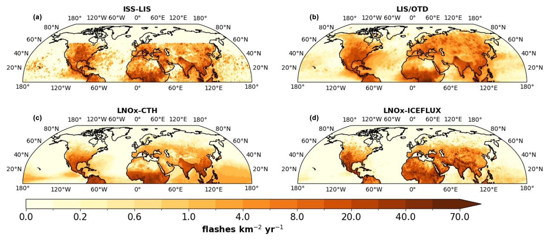
Figure 1 Spatial distribution of annual flash rates (flashes km⁻² yr⁻¹) over the NH based on (a–b) observations from (a) ISS-LIS satellite for the year 2018 (domain: 0–55° N) and (b) LIS/OTD climatology data (May 1995 to December 2014) and (c–d) simulation experiments from (c) LNOx-CTH and (d) LNOx-ICEFLUX.

As observed from our study, warm tropical regions (0–30° N), especially central Africa, South America, India, and southern China are the regions with high lightning flash rates due to large convective activity, followed by the mid-latitudes (30–60° N; Fig. 1c and d). South Asia, including India and southern China, where significant flash rates are observed, are known to exhibit the greatest seasonal and interannual variation in lightning activities (Pawar et al., 2012a; Xu et al., 2023). The annual flash rate is observed as 10–20 flashes km⁻² yr⁻¹ from both experiments, over most of the tropical lands (Fig. 1c and d), which is in agreement with the satellite observations from ISS-LIS and LIS/OTD (Fig. 1a and b). Over the mid-latitudes, flash rates are observed in the range of 2–4 flashes km⁻² yr⁻¹, while the polar regions (60–90° N) exhibit significantly lower values (0.1–0.2 flashes km⁻² yr⁻¹) as indicated by the simulations as well as the satellite observations. Therefore, the tropical and mid-latitude land regions dominate lightning activity. The spatial distribution of flash rates closely resembles the patterns observed in previous model-based studies using CTH and ICEFLUX schemes (Luhar et al., 2021; Gordillo-Vázquez et al., 2019; Finney et al., 2014, 2016a; Murray, 2016). However, patches of high flash rate observed in satellite data over central Canada, the central and southeastern parts of the USA, central European countries, and northern Russia are not reflected in the modelled flash rates from either experiment. Additionally, the elevated flash rates over central Asia are not captured in the LNOx-CTH simulation. Flash rates over land are significantly higher than the oceans due to intense convection over land regions (Albrecht et al., 2016). In oceanic regions, relatively higher flash rates (1–2 flashes km⁻² yr⁻¹) are observed in the tropical regions, particularly over the Bay of Bengal and the Pacific Ocean, as simulated in the LNOx-CTH experiment. Previous studies have reported inconsistencies in the equation for oceanic flashes developed by Price and Rind (1992) (Michalon et al., 1999; Boccippio, 2002; Luhar et al., 2021). However, our study demonstrates an improved flash rate distribution over tropical oceans, using the CTH scheme with a correction factor of 0.5 applied to constant b in Eq. (1), for the oceanic grids. A simulation with the original scheme by Price and Rind (1992) showed an overestimated flash rate over the tropical ocean by a factor ≈ 2, which is lowered to 1.3–1.4 after application of the correction factor in the present study. On the other hand, the magnitude of oceanic flash rates are significantly lower in simulations using the ICEFLUX scheme compared to the CTH scheme. The ICEFLUX scheme explicitly relates lightning flash rates to the upward ice flux; therefore, the weaker updraught strength in oceanic storms leads to less-efficient charge separation, resulting in fewer lightning flashes over the ocean (Finney et al., 2014).

Table 2 Mean annual flash rate over the NH, lands in the NH, and ocean in the NH for three latitude bands. Latitudinal coverage for the lightning data from ISS-LIS is 0–55° N.

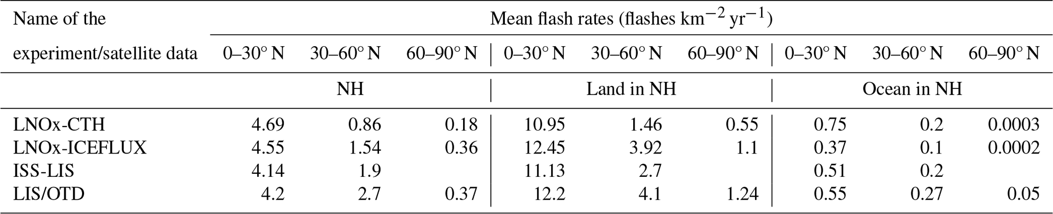
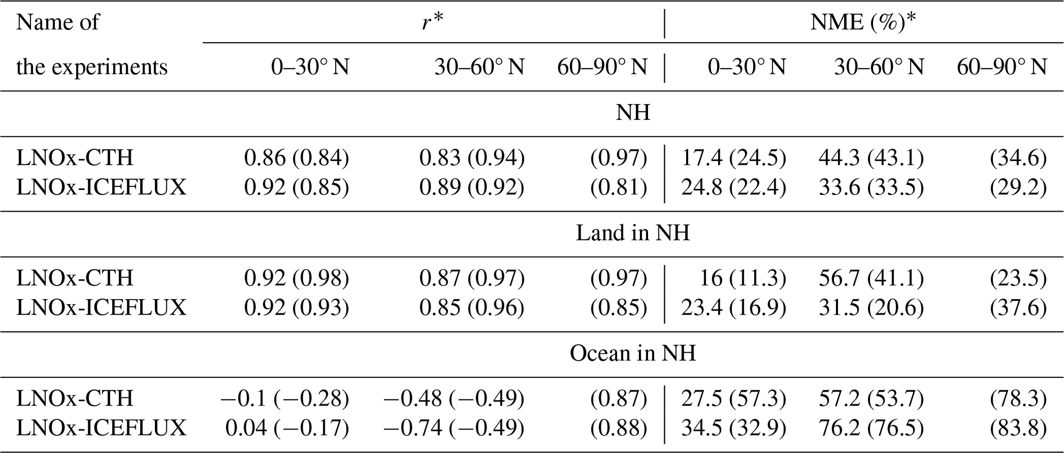
Table 3 Statistical analysis of spatially varying annual flash rates from the model compared with ISS-LIS and LIS/OTD satellite observations over the NH, land in the NH, and ocean in the NH for three latitude bands. Latitudinal coverage for the ISS-LIS data is 0–55° N. Statistical scores for comparison of simulated flash rates with LIS/OTD observations are provided in parentheses.

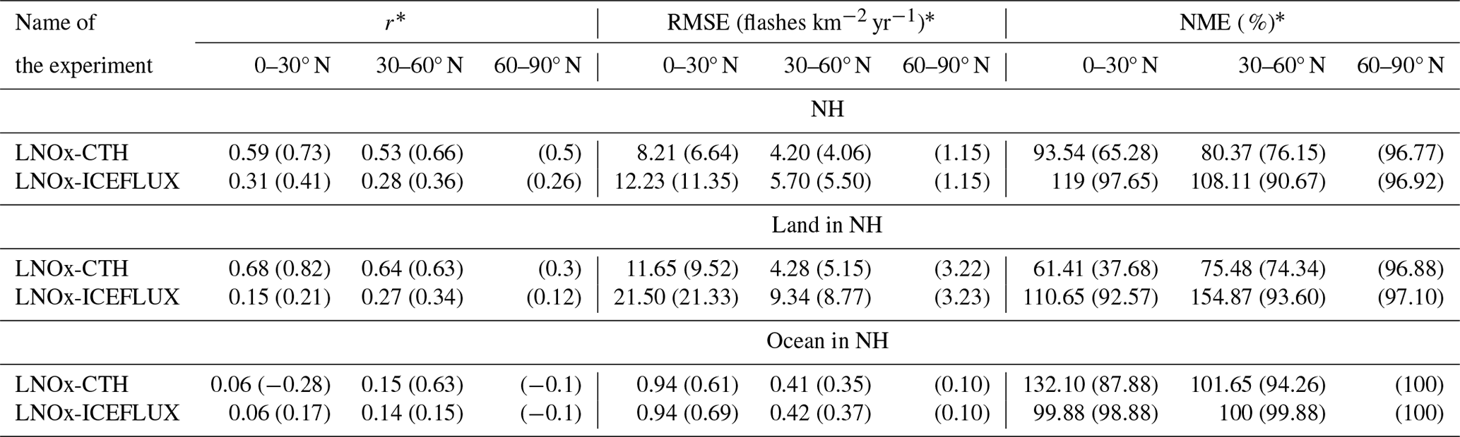
^* Correlation coefficient (r), RMSE, and NME are estimated by comparing simulated flash rates and ISS-LIS and LIS/OTD satellite observations for the spatially varying annual mean flash rates.

The spatial mean of annual flash rate over the NH tropics and NH tropical lands are comparable from two experiments, whereas the flash rate from LNOx-CTH is lower than that from LNOx-ICEFLUX by a factor of 2 at mid-latitudes (Table 2). These flash rates over the tropics are 5–8 times higher than the mid-latitudes for NH and lands, as estimated from the experiment with CTH. These factors are comparatively lower from the experiment with ICEFLUX and from the satellite observations, explaining the effectiveness of the ICEFLUX scheme over CTH in capturing flashes over the mid-latitudes. While the CTH scheme provides a useful approximation, since deeper convection generally correlates with higher lightning activity, it likely does not capture the full complexity of the processes driving lightning generation. Factors, such as updraught strength, cloud depth, ice water content, and mixed-phase regions play critical roles in charge separation and lightning production. By strictly capping cloud heights at the tropopause in the CTH scheme, the model may indeed underestimate flash rates in the mid-latitudes. This highlights the need to consider a multi-parameter approach for estimating flash rates, incorporating updraught dynamics, cloud microphysics, and ice-phase processes alongside cloud-top height. The ICEFLUX scheme, by explicitly modelling ice fluxes, provides a more realistic approach in predicting charge separation and lightning activity (Finney et al., 2014). This leads to improved flash rate estimations, particularly in mid-latitude storms where vertical motion, ice microphysics, and latent heat fluxes play a complex role in thunderstorm electrification. Spatially mean annual flash rates over tropical lands from both experiments are close enough to the satellite measurements in the tropics over the NH and lands, while at mid-latitudes only a good resemblance is observed for data from LNOx-ICEFLUX. On the other hand, the simulation with the CTH scheme estimates the flash rates over tropical ocean as almost twice that of those estimated using the ICEFLUX scheme, unlike what is shown in previous studies (Finney et al., 2016b). We compare the spatially varying simulated annual flash rates with satellite observations (ISS-LIS and LIS/OTD), and the corresponding statistical metrics are presented in Table 3. Correlation coefficients for spatially varying flash rates show comparatively stronger correlations over the tropics and mid-latitudes of the NH and land regions, between that from LNOx-CTH and satellite data, compared to LNOx-ICEFLUX, being consistent with the findings by Clark et al. (2017). The flash rates from LNOx-CTH exhibit significantly higher correlations, particularly when evaluated against LIS/OTD data. Analysis of RMSE and NME also indicates lower errors for LNOx-CTH over these regions in comparison to those observed for LNOx-ICEFLUX, indicating the spatial variations of flashes from the first experiment align well with the satellite data. The worst performance is observed in the polar lands compared to the other two latitude bands, as well as over oceanic regions from both experiments, characterized by weak correlations and higher errors. Hence, both schemes struggle to accurately simulate flash rates over oceans and high-latitude lands. However, since lightning activity is minimal in these regions, the impact of this limitation is relatively minor. These results also underscore the ongoing challenges of accurately representing convection and capturing lightning flashes over the oceans. In summary, the statistical analysis points out the effectiveness of the LNOx-CTH scheme in reproducing the spatially varying lightning flashes reasonably well, particularly in the tropics over the NH and lands. However, both schemes exhibit limitations in the polar regions and over oceans, indicating scopes for further improvement in the parameterizations. While LNOx-ICEFLUX provides a reasonable estimate of flash rate magnitudes over both the tropics and mid-latitudes, it struggles to accurately capture the observed spatial pattern of lightning flashes, emphasizing the need for further improvement.

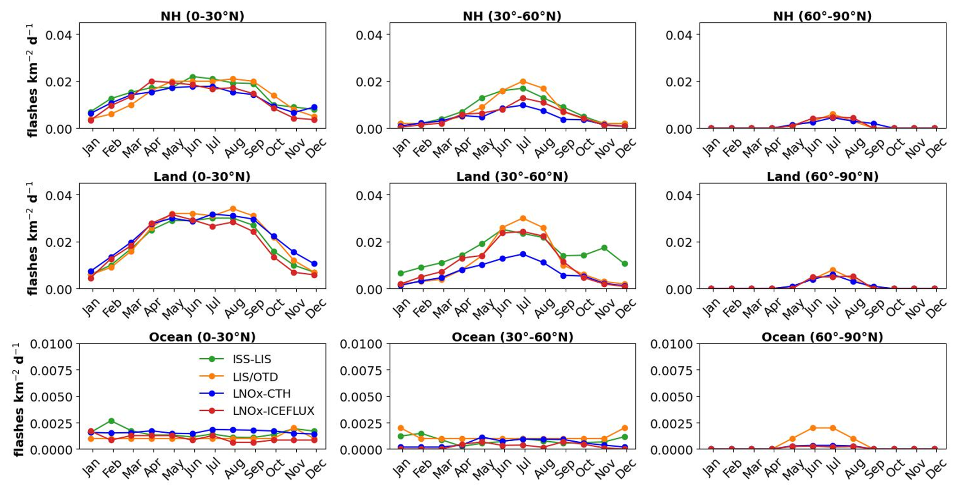
Figure 2 Comparison of monthly mean flash rates (flashes km⁻² d⁻¹) from simulations (LNOx-CTH and LNOx-ICEFLUX) with ISS-LIS satellite observations for the year 2018 (domain: 0–55° N) and LIS/OTD monthly climatology (May 1995 to December 2014), over the NH, land, and ocean in NH for the three latitude bands. Please note that the y axis in the plots for oceans is presented on a different scale.

Figure 2 compares the monthly averaged lightning flash rates across different latitude bands in the NH, land, and ocean regions. The figure incorporates satellite observations (ISS-LIS and LIS/OTD) and results from two simulation experiments (LNOx-CTH and LNOx-ICEFLUX). Flash rates from the LNOx-CTH experiment show a clear seasonal cycle, with peaks occurring in May–August over the NH and land. During the winter months (November–January), flash rates drop significantly, being 5–7 times lower than the summer (May–August) peak values. The seasonal variation observed in the LNOx-ICEFLUX experiment and satellite observations closely align with this trend. Over land, both observations and simulations indicate high flash rates, particularly in the tropics, followed by mid-latitudes for all the months. Peak lightning activity over land occurs during late spring and early summer (May–August), corresponding to enhanced convective activity (Holle et al., 2016; Ghosh et al., 2023). In contrast, flash rates over oceans are consistently lower over all latitude bands. The tropical ocean shows a uniform flash rates throughout the year, without any prominent seasonality. The delay in the seasonal peak of flash rates over the NH with CTH, and particularly with ICEFLUX, as noted by Finney et al. (2014), is not seen in our simulations. Therefore, using near real-time, high spatially and temporally resolved meteorological data from ECMWF-IFS with continuous updates and improved configuration for advection in CHIMERE, we achieve an improved seasonal distribution that match well with the satellite measurements.

Table 4 Statistical analysis of monthly mean flash rates from the model compared with ISS-LIS and LIS/OTD satellite observations over the NH, land in the NH, and ocean in the NH for three latitude bands. Statistical scores for comparison of simulated flash rates with LIS/OTD observations are provided in parentheses.

^* Correlation coefficient (r) and NME estimated by comparing simulated monthly mean flash rates and the same from ISS-LIS and LIS/OTD satellite observations.

The modelled monthly mean flash rates from the simulations exhibit a strong positive correlation with satellite observations (ISS-LIS and LIS/OTD), with correlation coefficients ranging from 0.85 to 0.97 (Table 4). This agreement is consistent across all latitude bands over the NH, land regions, and the polar ocean region from both experiments (LNOx-CTH and LNOx-ICEFLUX). These findings indicate that the simulations successfully capture the seasonal variability of flash rates. In contrast, a weaker negative temporal correlation is observed over tropical and mid-latitudinal oceans, indicating an inverse relationship between simulated and observed seasonality in flash rates in these regions. When comparing the simulated monthly flash rates with satellite observations, the results from LNOx-CTH align more closely with satellite observations for the tropics than the mid-latitudes, as evidenced by lower NME for the tropics over the NH, land, and ocean regions. Notably, the simulation LNOx-ICEFLUX exhibits a better performance at mid-latitudes than the LNOx-CTH experiment, over the NH and land regions, especially when compared with LIS/OTD measurements. Further, advancement in the seasonal representation of oceanic convection processes is essential for improving the simulation of flash rates over oceans.

Table 5 Estimated flash frequencies and LNO_x emissions from simulations over the NH. Flash frequencies in parentheses are estimated for the domain 0–55° N, comparable to the ISS-LIS satellite data (23.6 flashes s⁻¹). The flash frequencies from the LIS/OTD climatology data are 26.4 and 25.3 flashes s⁻¹ over the NH and for the domain 0–55° N.

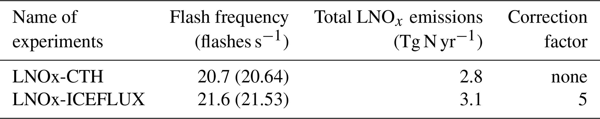
Table 6 Statistical analysis comparing simulated mixing ratio at surface to the ground-based observations for O₃ and NO₂. The positive and negative values of MAB show that the simulated surface concentration is higher and lower than the observations, respectively.

The annual flash frequencies over the NH are estimated as 20.7 and 21.6 flashes s⁻¹, respectively, from the LNOx-CTH and LNOx-ICEFLUX experiments (Table 5). These values are consistent with the satellite observations (23.6 and 26.4 flashes s⁻¹, respectively, from ISS-LIS and LIS/OTD observations over the NH) as well as to those obtained in recent model-based studies over the NH (Luhar et al., 2021). While no scaling factor is applied in the simulated flash rates from LNOx-CTH, the flash frequency from LNOx-ICEFLUX is divided by a factor of 5 to reconcile with the satellite-observed frequency. Accordingly, the evaluation of the results from LNOx-ICEFLUX has been conducted using flash rates adjusted by this factor. For instance, a recent study by Finney et al. (2016a) utilizing the UK Chemistry and Aerosol (UKCA) model determined that the global flash rate scaling factors required for the UKCA model are 1.44 and 1.12 for the CTH and ICEFLUX lightning parameterizations, respectively. Another study by Gordillo-Vázquez et al. (2019) produced scaling factors of 2.05 and 4, respectively, for the CTH and ICEFLUX lightning schemes in the Community Atmosphere Model (CAM5). A study by Tost et al. (2007) reported that scaling factors may vary by up to 2–3 orders of magnitude, depending on the lightning parameterization used and the resulting flash rate, to better match the observations. Uncertainties in the estimated lightning frequency may arise from the input meteorological data and model configuration, and the detection efficiency of satellite measurements is also a significant factor when comparing the modelled flashes with satellite observations (Blakeslee et al., 2020; Erdmann et al., 2020; Zhang et al., 2023).

3.2 NO_x emissions from lightning

The production of LNO_x emissions depends on the average flash frequency (in flashes s⁻¹) and the NO_x production efficiency per flash, which represents the rate of NO_x emissions per flash (Schumann and Huntrieser, 2007; Gordillo-Vázquez et al., 2019; Bucsela et al., 2019; Luhar et al., 2021). In this study, the mean LNO_x emission per flash is estimated as 332 mol. The estimated annual NO emissions from lightning are 2.8 and 3.1 Tg N yr⁻¹ over the NH, respectively, from LNOx-CTH and LNOx-ICEFLUX simulations (Table 5). Notably, LNO_x emission from LNOx-ICEFLUX is 7.5 % higher than that from LNOx-CTH. Recent studies estimate global LNO_x emissions typically range from 2 to 8 Tg N yr⁻¹ (Schumann and Huntrieser, 2007; Finney et al., 2016b; Nault et al., 2017), with variations reaching up to 25 Tg N yr⁻¹ in extreme scenarios (Price et al., 1997a, b). Price et al. (1997b) suggested that the global annual LNOx emissions cannot be less than 5 Tg N or exceed 25 Tg N. The LNOx emissions from our study align well with the estimates by Luhar et al. (2021), which ranged from 2.39 to 3.41 Tg N yr⁻¹ over the NH when using CTH and a new parameterization by Luhar et al. (2021). A recent study shows that the estimated global LNO_x emissions, with the CTH scheme and the new parameterization by Luhar et al. (2021), are, respectively, 5.66 and 5.58 Tg N yr⁻¹ in the model EMAC (Pérez-Invernón et al., 2024). These estimates are, respectively, 17 % higher and 15 % lower than that estimated by Luhar et al. (2021) with the same parameterizations, showing that the LNO_x emissions are highly sensitive to the model configurations. The monthly variation in LNO_x emissions, in our study, from the two simulations is shown in Fig. 3a. The results indicate that peak emissions occur in July–August, followed by May–June and September, in the LNOx-CTH experiment. The emissions from the LNOx-ICEFLUX experiment peak in May, followed by the remaining summer months (April, June–August). Approximately 60 %–70% of the total annual LNO_x emissions are contributed during late spring and summer (April–August), when lightning activity is at its highest.

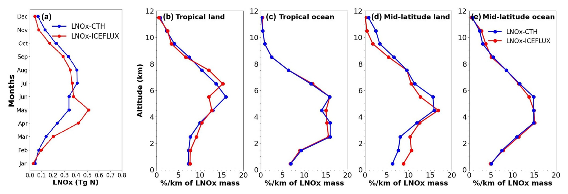
Figure 3 (a) Monthly LNO_x emissions (in Tg N) from simulations LNOx-CTH and LNOx-ICEFLUX. (b–e) Vertical distribution of percentage of annual LNO_x mass per kilometre from simulations LNOx-CTH and LNOx-ICEFLUX averaged over (b) tropical land, (c) tropical ocean, (d) mid-latitudinal land, and (e) mid-latitudinal ocean.

Figure 3b–e represent the vertical distribution of LNO_x emissions as percentage of LNO_x mass per kilometre. The emissions from CG and IC flashes are calculated separately considering CG flashes only below the freezing level and the IC flashes only above the freezing level and below the cloud top. A simple vertical structure of the emissions is adopted in this study, considering the emissions to be evenly distributed over an altitude range. The distribution shows the maximum of LNO_x mass lies between the altitude range of 4–7 km at all regimes from both simulations, showing the typical backward C-shape (Ott et al., 2010); 60 %–65 % of LNO_x mass is injected at this altitude range. Here, it is to be mentioned that annually 1.85 and 1.9 Tg N LNO_x are being generated over tropical land as obtained from LNOx-CTH and LNOx-ICEFLUX simulations, respectively, being almost 63 %–66 % of total annual LNOx over the NH. The amounts are 0.55 (0.76), 0.15 (0.09), and 0.07 (0.03) Tg N for mid-latitudinal land, tropical ocean, and ocean and mid-latitudinal ocean, respectively, from the LNOx-CTH (LNOx-ICEFLUX) simulation. Therefore, the mid-tropospheric region (4–8 km) contributes the maximum to the LNOx mass, especially over the tropical land region. The vertical profiles available from previous studies, e.g., Pickering et al. (1998); Ott et al. (2010); Luhar et al. (2021), reveal a similar shape for all the profiles but contributing a maximum at the upper-tropospheric region (within 2–4 km of the tropopause) rather than middle troposphere. However, the study by Pickering et al. (1998) presents a high emission near the surface due to a strong downdraught, where the distribution is low and almost uniform up to 5–6 km as observed from the studies by Ott et al. (2010) and Luhar et al. (2021). Nevertheless, the profile over mid-latitude lands from our study matches well with that from the study by Ott et al. (2010), with a maximum at 5 km. In our study, 13 %–19% of total LNO_x mass is estimated from the surface up to 2 km over tropical and mid-latitude lands and tropical oceans. LNO_x production is suggested to be proportional to atmospheric pressure by Goldenbaum and Dickerson (1993) and Pickering et al. (1998). The vertical distribution of LNO_x mass can be improved by replacing the simple distribution currently used with the more detailed scheme developed by Pickering et al. (1998).

3.3 Vertical distribution of gases: effects of LNO_x

3.3.1 Ozone

Numerous studies have demonstrated that LNO_x emissions play a significant role in influencing the levels of ozone and other trace gases as a result of the oxidation of CO, CH₄, and volatile organic compounds (VOCs), particularly in the free troposphere (Luhar et al., 2021; Mao et al., 2021; Finney et al., 2016b; Liaskos et al., 2015). The changes in the annual mean of O₃ mixing ratio, due to the inclusion of LNO_x in simulation LNOx-CTH, with respect to that from simulation noLNOx, averaged over four altitude bands (998–900, 900–750, 750–500, and 500–200 hPa), are presented in Fig. 4. The same changes from experiment LNOx-ICEFLUX with respect to LNOx-CTH are also produced in Fig. 5. The highest increase in simulated O₃ is observed in the altitude band 750–500 hPa, specifically over the tropics, by 6–10 ppbv. And a 4–6 ppbv increase over the tropics is also observed at the altitude bands 900–750 and 500–200 hPa (middle to upper troposphere). The increase in O₃ is at a maximum over the tropical region of America, central Africa, southern Asia, and the Maritime Continent in Southeast Asia (Indonesia, the Philippines, and Malaysia). The above-mentioned regions with comparatively larger increase in O₃, identified for all the altitude bands, are observed as regions with the largest convection depth and LNO_x emissions (Banerjee et al., 2014). A higher value by 2–4 ppbv in annual mean O₃ is also observed from LNOx-ICEFLUX with respect to LNOx-CTH over the tropical region for the altitude band 750–500 hPa, followed by the 900–750 hPa band (Fig. 5); an even higher increase over the tropical region of America, central Africa, and the Tibetan Plateau is also found from LNOx-ICEFLUX. On the other hand, the changes in O₃ mixing ratio are insignificant over mid-latitude and polar regions from both simulations with respect to noLNOx. The percentage changes in the annual mean of O₃ mixing ratio from LNOx-CTH with respect to noLNOx, averaged over selected latitude and altitude bands, present an overall improvement in tropospheric O₃ (Table S2 in the Supplement). O₃ levels are significantly elevated by 10 %–19 % in the middle and upper troposphere (750–200 hPa), where O₃ production occurs efficiently (Dahlmann et al., 2011). Tropical middle- and upper-troposphere regions are more crucial in O₃ production as most lightning discharges occur in these regions (Luhar et al., 2024; Bucsela et al., 2019; Murray, 2016). A moderate (3 %–5%) to low (1 %–2 %) increase in annual mean of middle- and upper-tropospheric O₃ is also observed over mid-latitudes followed by the polar region. The increase is comparatively higher during late spring and early summer (May–August), being 6 %–15 % over mid-latitudes and 2 %–4 % over polar regions. Higher annual mean values of O₃ mixing ratios are observed in LNOx-ICEFLUX compared to LNOx-CTH in the middle to upper troposphere across all latitude bands, likely due to comparatively higher LNO_x production from LNOx-ICEFLUX in these regions.

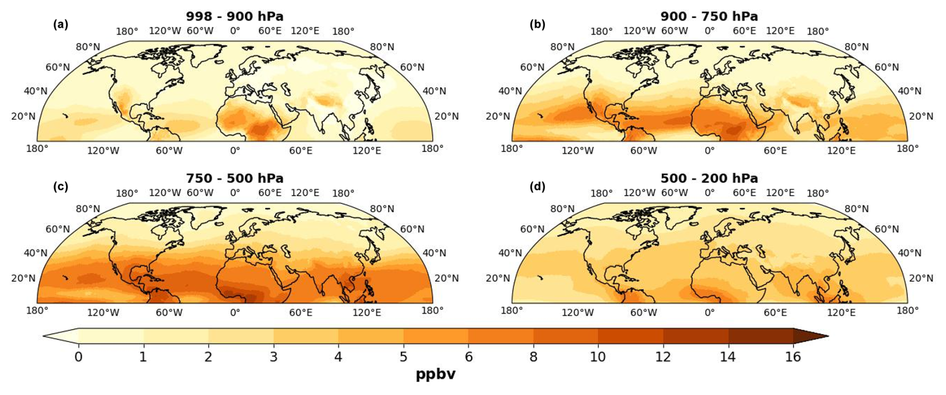
Figure 4 Changes in annual mean of O₃ mixing ratio from experiment LNOx-CTH with respect to noLNOx (ΔO₃) at the altitude bands of (a) 998–900 hPa, (b) 900–750 hPa, (c) 750–500 hPa, and (d) 500–200 hPa; positive and negative values represent the increase and decrease in the O₃ mixing ratio, respectively.

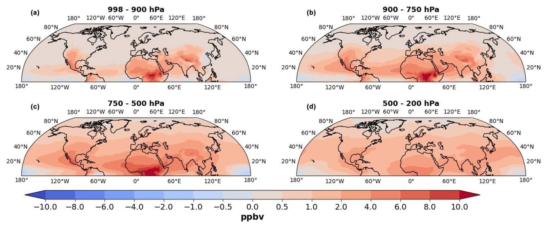
Figure 5 Changes in annual mean of O₃ mixing ratio from experiment LNOx-ICEFLUX with respect to LNOx-CTH at the altitude bands of (a) 998–900 hPa, (b) 900–750 hPa, (c) 750–500 hPa, and (d) 500–200 hPa; positive and negative values represent the increase and decrease in the O₃ mixing ratio, respectively.

Figure 6 represents the vertical profile of annual mean O₃ mixing ratio from simulations and their comparison with the WOUDC ozonesonde measurements, averaged for the stations over three latitude bands (0–30° N, 30–60° N, and 60–90° N). The upper-tropospheric O₃ mixing ratio is moderately higher than that observed at the surface for the tropics by 30 %–60 %, while it is 2–3 times higher over the mid-latitudes and polar region as observed from simulation LNOx-CTH (Table S2). The upper-tropospheric O₃ over the polar region is also almost twice that over the tropics (Table S2). Notably, the vertical profile from observations represents an increasing O₃ mixing ratio with altitude, whereas those from simulations show an overestimated O₃ mixing ratio near the surface, which tend to decrease near the boundary layer in the tropics (Fig. 6). The simulated O₃ is also observed to be higher near the surface and show a continuous increasing pattern over mid-latitude and polar regions. It is seen in Fig. 6 that the simulated O₃ mixing ratio from the experiments with LNO_x represents the measured O₃ adequately well, specifically in the free troposphere over the tropics, where a large underestimation is observed in simulated O₃ from the noLNOx simulation. The absolute bias in simulated O₃ in the free troposphere, especially over the tropics, is reduced due to inclusion of LNO_x in the model (Table S3). The bias is, however, lower for that from LNOx-CTH in comparison to LNOx-ICEFLUX. O₃ production efficiency due to LNO_x is higher in the mid-to-upper troposphere, primarily because lower temperatures extend the lifetime of NO_x, while enhanced photolysis rates further favour O₃ accumulation (Labrador et al., 2005). The high underestimation in the simulated O₃ mixing ratio in the altitude band 500–200 hPa, i.e., the upper troposphere and lower stratosphere, over mid-latitudes and polar regions still exists, even after the inclusion of LNO_x; however, lower underestimation is observed for LNOx-ICEFLUX. The underestimation suggests that the modelled stratosphere–troposphere exchange still requires significant refinement, and the cross-tropopause transport may not be adequately resolved due to the low model top.

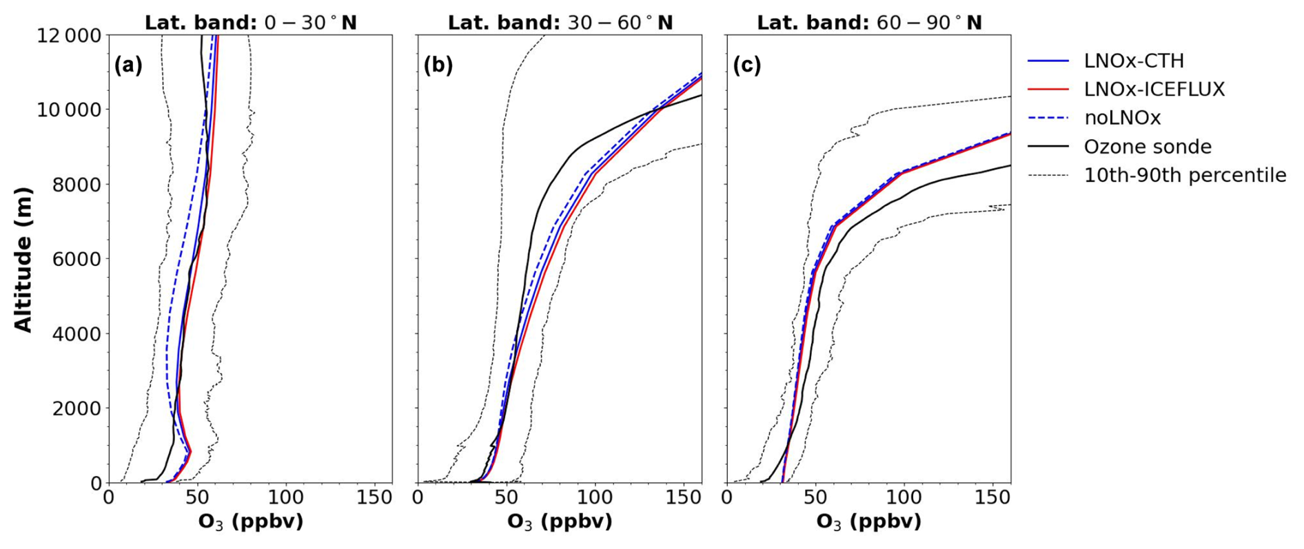
Figure 6 Vertical profile of annual mean of O₃ mixing ratio from noLNOx (dashed blue line), LNOx-CTH (blue solid line), and LNOx-ICEFLUX (red solid line) simulations and comparison with the WOUDC ozonesonde measurements (black solid line), averaged for the stations over the latitude bands (a) 0–30° N, (b) 30–60° N, and (c) 60–90° N; the dashed black lines indicate the 10th and 90th percentiles of the WOUDC ozonesonde-measured values.

We also compare the vertical profiles of simulated O₃ with those from SHADOZ ozonesonde-measured data at the stations of Kuala Lumpur, Hanoi, Costa Rica, and Hilo, situated over the NH tropics. The plots are provided in the Supplement (Fig. S1). Among the stations, at Kuala Lumpur the simulated O₃ profile from LNOx-ICEFLUX shows a good match with the observations for the free troposphere, while the profile from LNOx-CTH aligns well with observations at Costa Rica. However, the modelled O₃ profiles show underestimation and overestimation at most of the altitudes, respectively, at Hanoi and Hilo, but overall they replicate the observed altitudinal distribution quite well. The comparisons once again represent the effect of LNO_x on O₃, specifically for the free troposphere.

The monthly comparison of simulated O₃ from the LNOx-CTH and LNOx-ICEFLUX experiments with WOUDC ozonesonde measurements is presented in Fig. S2, across two altitude (750–500 and 500–200 hPa) and three latitude bands. The monthly variation reveals the highest peaks during March and October in the tropics, with the lowest levels observed during June–July for both altitude bands. A similar variation is noted at mid-latitudes and in the polar regions for the 750–500 hPa altitude band, aligning well with the observed monthly trends. The simulated O₃ from both experiments closely matches the observed values for the tropics and mid-latitudes for both altitude bands, exhibiting a low bias of ±3–10 ppbv. However, an overestimation of simulated O₃ is apparent during January–April, particularly over the tropics. While there is a good agreement between simulated and observed O₃ over the polar region for the 750–500 hPa altitude band, a significant underestimation of simulated O₃ is evident in the 500–200 hPa altitude band as discussed previously.

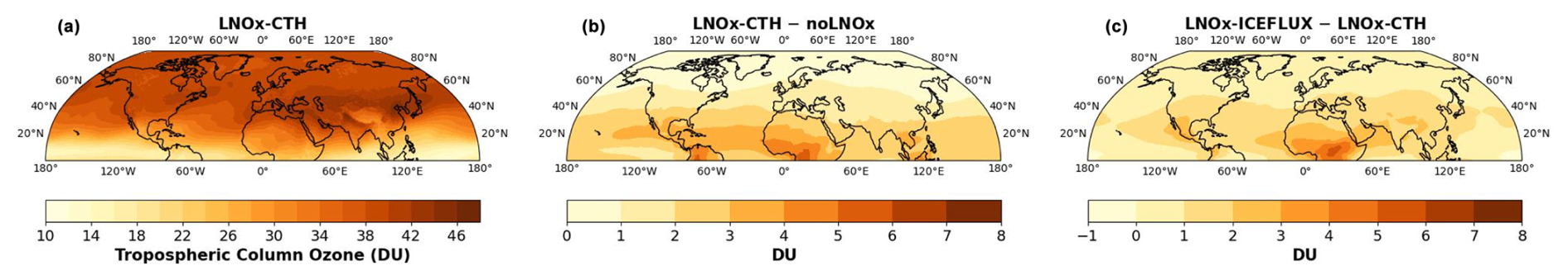
Figure 7 (a–c) Spatial distribution of (a) simulated tropospheric column of ozone (TCO) in DU (Dobson unit), over the NH from experiment LNOx-CTH, (b) changes in simulated TCO from experiment LNOx-CTH with respect to noLNOx simulation, (c) differences in simulated TCO from experiment LNOx-ICEFLUX with respect to LNOx-CTH; positive and negative values represent the increase and decrease, respectively.

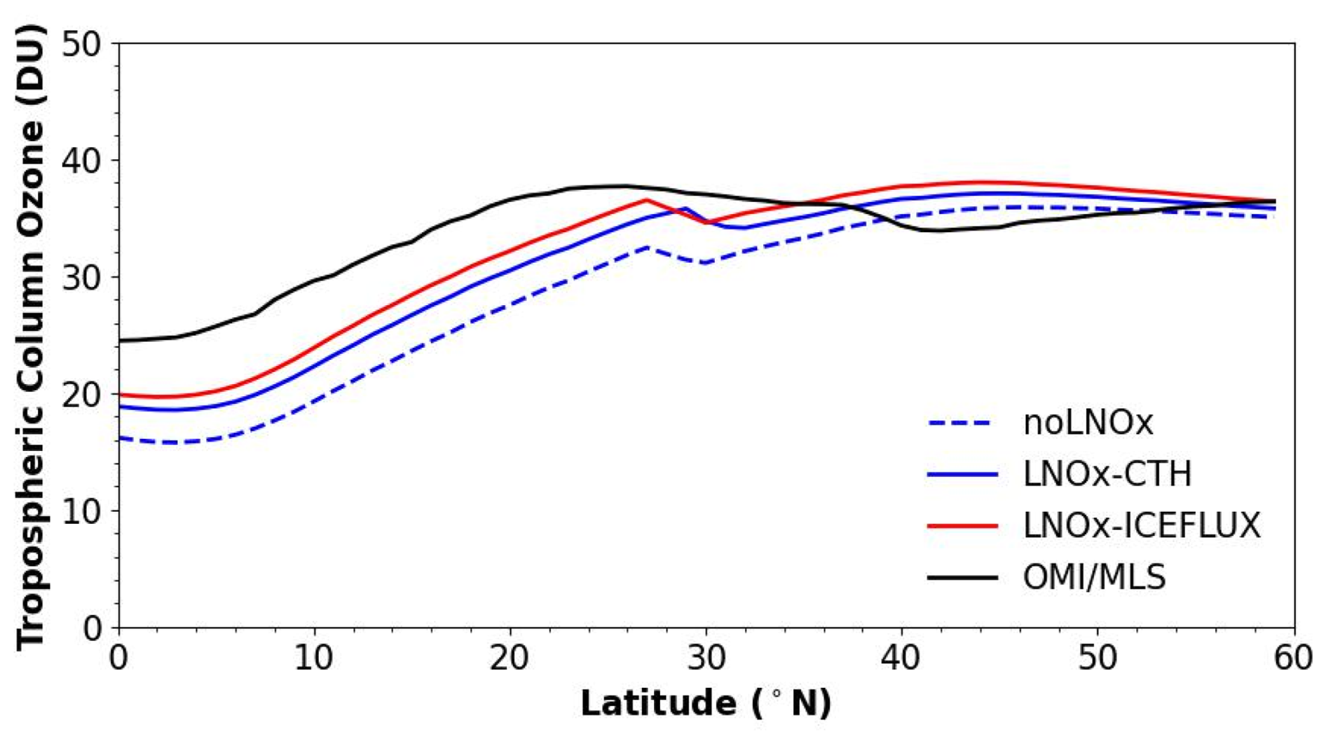
Figure 8 Zonal average of TCO from simulations over the NH and its comparison with the same from OMI/MLS.

The spatial distributions of the tropospheric column of ozone (TCO) from the LNOx-CTH simulation, along with the changes in TCO relative to the noLNOx and LNOx-ICEFLUX simulations, are shown in Fig. 7. The TCO is observed to increase from the tropics toward higher latitudes, with the higher values occurring over the mid-latitudes (32–42 DU, Dobson unit), particularly over Asian countries (40–44 DU; Fig. 7a). The lower TCO values in the tropics are attributed to the model’s top height being lower than the tropopause height in this region (refer to the Table S1 in the Supplement, presenting the tropopause height). The TCO from the LNOx-CTH simulation is higher by 2–4 DU for the tropics than that from the noLNOx simulation, while the LNOx-ICEFLUX simulation produces even higher TCO values compared to LNOx-CTH, especially over the tropics (Fig. 7b–c). The tropospheric O₃ burdens, estimated from the simulation LNOx-CTH and LNOx-ICEFLUX, are, respectively, 176 (150) Tg and 182 (155) Tg, over the NH and over the domain of 0–60° N (presented inside parentheses). These burdens represent a 7 %–11 % increase relative to the noLNOx simulation (Table 8). Notably, the estimated O₃ burden in this study aligns closely with observations from OMI/MLS (159 Tg) for the domain of 0–60° N. The spatial distribution of TCO from OMI/MLS is shown in Figure S3 in the Supplement. A comparison of the zonal mean TCO over 0–60° N reveals good agreement between the simulated TCO and OMI/MLS observations in the mid-latitudes (Fig. 8). However, the simulations underestimate TCO in the tropics by 7 %–26 %, owing to the limited model top height, which excludes part of the troposphere above it. Despite this limitation, incorporating LNO_x into the model leads to significant improvements in simulated TCO.

3.3.2 NO₂

Figure 9a represents the spatial distribution of NO₂ column density estimated from LNOx-CTH. A high NO₂ column density of 2–3 × 10¹⁵ molec. cm⁻² is observed over southern and eastern Asia (India and eastern China), northwest Europe, and eastern parts of the USA. The spatial variation in NO₂ column matches well with that obtained from OMI observations (Fig. S4), highlighting elevated NO₂ column densities in countries with significant industrial activities (Cooper et al., 2022). A decrease in NO₂ column density (0.2–0.6 × 10¹⁵ molec. cm⁻²) due to inclusion of LNO_x emissions is primarily observed over the above-mentioned regions with high NO₂ pollution (Fig. 9b). The inclusion of LNO_x in the model increases large-scale O₃ and OH concentrations, therefore reducing the lifetime of NO_x through oxidation reactions with HO_x including OH (Labrador et al., 2005; Schumann and Huntrieser, 2007). Figure S5 in the Supplement depicts the increase in HNO₃ column density over the above-mentioned region, supporting the fact that NO₂ is oxidized and converted to HNO₃, increasing the column density of HNO₃. Hence, rapid conversion of NO₂ into other compounds, such as HNO₃, leads to its subsequent removal and a net decrease in NO₂ column density over the regions with high anthropogenic pollution. Figure S6, showing changes in annual mean NO₂ mixing ratio (in ppbv) from experiment LNOx-CTH with respect to noLNOx, demonstrates a decrease in NO₂ by 0.1–0.3 ppbv over the regions with higher anthropogenic NO₂ pollution as mentioned above, at the altitude band of 998–900 hPa, i.e., mostly near the surface followed by the altitude band 900–750 hPa. A very small increase (0.05 ppbv) is observed over most parts of the NH at the higher-altitude bands (750–500 and 500–200 hPa), due to inclusion of LNO_x emissions. Overall, the NO₂ column density decreases over the regions with high anthropogenic pollution. Again, small increases of 0.1–0.3 × 10¹⁵ molec. cm⁻² are observed over Africa, South America, Southeast Asia, the Maritime Continent, and the tropical oceans, where NO₂ pollution is relatively lower (Fig. 9a and b). Notably, NO₂ column densities from LNOx-ICEFLUX are higher by 0.6–0.8 × 10¹⁵ molec. cm⁻² compared to LNOx-CTH over southern Asia, central Africa, and parts of the United States (Fig. 9c).

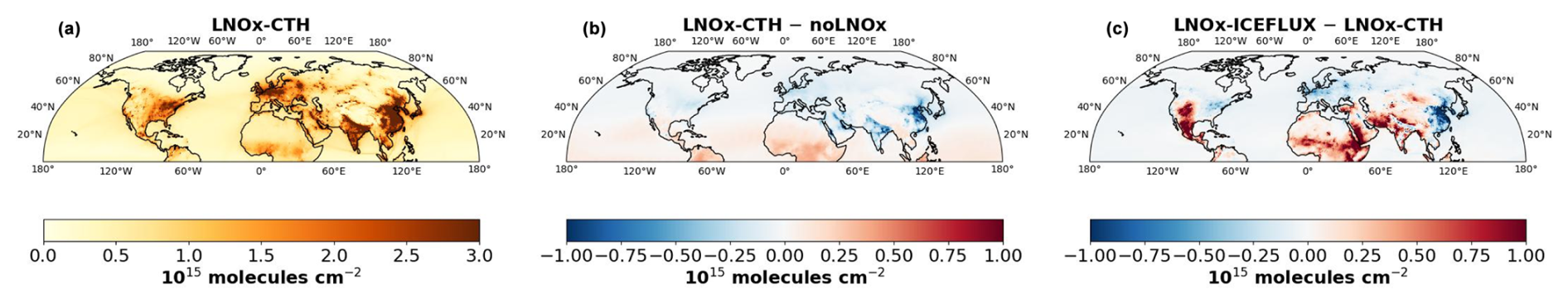
Figure 9 (a–c) Spatial distribution of (a) simulated NO₂ column density in 10¹⁵ × molec. cm⁻², over the NH from experiment LNOx-CTH, (b) changes in simulated NO₂ column density from experiment LNOx-CTH with respect to the noLNOx simulation, and (c) differences in simulated NO₂ column density from experiment LNOx-ICEFLUX with respect to LNOx-CTH; positive and negative values represent the increase and decrease, respectively.

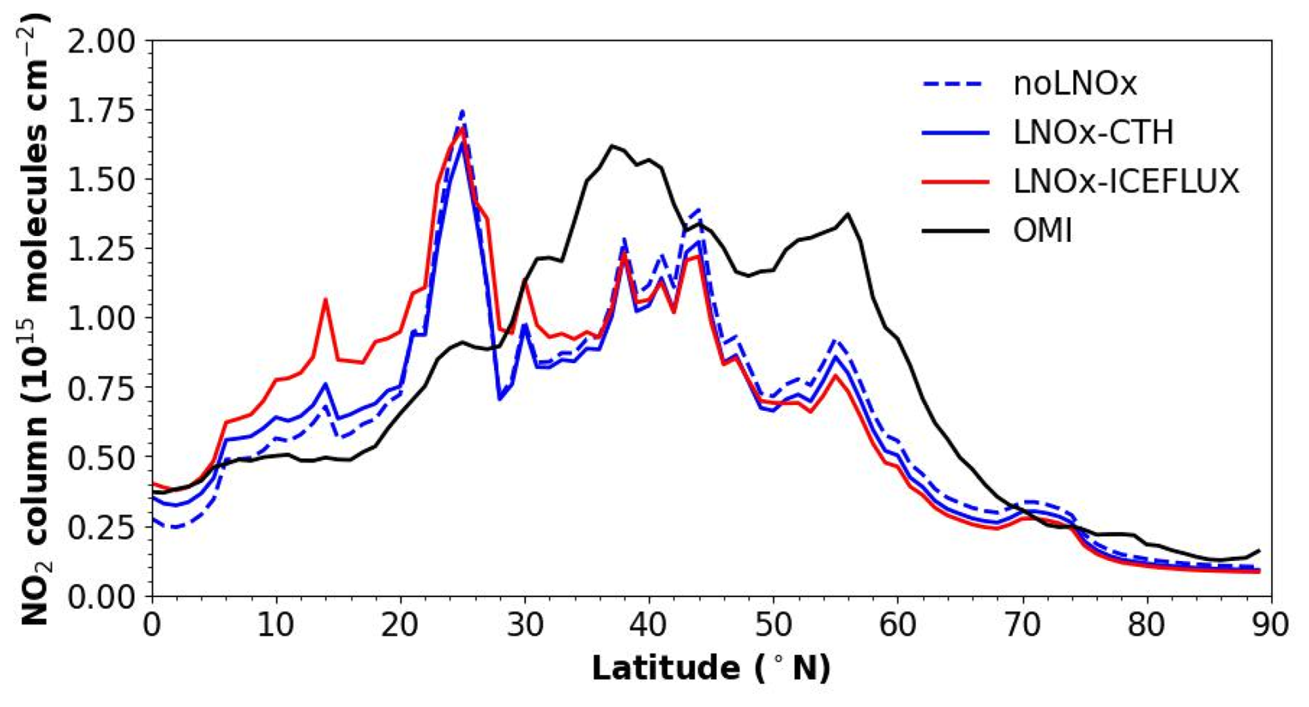
Figure 10 Zonal average of NO₂ column density from simulations over the NH and their comparison with the same from OMI.

The zonally averaged NO₂ column distribution (Fig. 10) reveals elevated column densities over the tropics, especially between 20–30° N, and the mid-latitudes, even in the absence of LNO_x emissions. The zonal averages range from 0.35–1.75 × 10¹⁵ molec. cm⁻² in these regions, which is nearly double the values observed at higher latitudes (60–90° N). The peak at 20–30° N (1.75 × 10¹⁵ molec. cm⁻²) is due to the high NO₂ column density estimated from simulations over southern and southeast Asia due to high NO₂ emissions from larger industrial activities. This peak is, however, not observed in OMI observations. On the other hand, a study by Luhar et al. (2021) has depicted that the NO₂ column density obtained from Copernicus Atmosphere Monitoring Service (CAMS) reanalysis data shows a peak of 1.5 × 10¹⁵ molec. cm⁻² at this latitude band (20–30° N), where OMI underestimates the NO₂ column density. The higher uncertainty in OMI-retrieved NO₂ columns, as compared with available satellite observations (GOME-2, SCIAMACHY, and TROPOMI) is considerable in this regard. The uncertainties are primarily due to instrumental errors, limitations of the OMI sensor in capturing the NO₂ below the cloud level, vertical profile assumptions, and surface reflectivity (Bucsela et al., 2013; Boersma et al., 2018). A secondary maximum in NO₂ column density is identified between 35–45° N from simulations as well as from satellite observations. However, the simulated NO₂ column density is underestimated at mid-latitudes by 20 %–40 %. At higher latitudes (60–90° N), where the magnitudes are comparatively lower, the simulated NO₂ column density matches well with satellite-based observations. Overall, the zonally averaged NO₂ column densities from the simulations closely replicate satellite observations, except for a pronounced peak at 20–30° N from simulated NO₂. The tropospheric burden of NO₂ is 146 Gg from LNOx-CTH, being comparable to that from noLNOx and 11 % lower than that estimated from OMI (Table 8). The burden estimated from LNOx-ICEFLUX is 3 % higher and 8 % lower than LNOx-CTH and OMI, respectively.

3.4 Impacts of LNO_x on surface-level O₃ and NO₂

The effect of LNO_x on surface-level O₃ and NO₂ over the NH is analysed in this section. The spatial distribution of the annual mean of O₃ mixing ratio and NO₂ at the surface from experiment LNOx-CTH and changes in the mixing ratio due to inclusion of LNO_x (ΔO₃ and ΔNO₂) are presented in Fig. 11a and d and Fig. 11b and e, respectively. Other than natural sources (e.g., lightning, soil-NO_x emissions), emissions from fossil fuel combustion for transportation, industrial activities, energy generation, and biomass burning also have a profound influence on tropospheric O₃ and NO₂ concentrations (Lelieveld and Dentener, 2000; van der A et al., 2008; Butler et al., 2020). In our study, the O₃ mixing ratio at the surface varies spatially with higher values ranging between 35–45 ppbv over the latitude band of 10–50° N, specifically over the land, being almost 1.5–2 times that observed over the rest of the NH. The NO₂ at the surface is within a range of 0.5–2 ppbv over most parts of the NH, showing higher magnitudes over the USA, western Europe, India, eastern China, and Japan (5–10 ppbv). To indicate the impact of LNO_x emissions on changes in surface-level O₃ and NO₂, the annual mean of mixing ratio obtained from experiment LNOx-CTH is compared with that from noLNOx. The positive and negative values of ΔO₃ and ΔNO₂ depict an increase and decrease, respectively, in surface mixing ratio (Fig. 11b and e). The study shows an overall increase in surface O₃ by 1–3 ppbv over most parts of the tropical lands and mid-latitudes up to 50° N (Fig. 11b), while the increase is almost negligible over 50–90° N (< 1 ppbv). A comparatively larger increase of 3–5 ppbv is observed over tropical parts of America and Africa and the Tibetan Plateau but is particularly noteworthy (5–10 ppbv) over the central part of Africa, which is a hotspot location with a high lightning flash rate (refer to Sect. 3.1). The O₃ level from LNOx-ICEFLUX is even higher (2–4 ppbv) than that estimated from LNOx-CTH (Fig. 11c). Unlike O₃, NO₂ exhibits both an increase and decrease in mixing ratio at the surface as an effect of lightning (Figure 11e) but by a lesser magnitude (0.01–0.1 ppbv). While the increase is observed over South America, Africa, the Maritime Continent, and Southeast Asia, a decrease in NO₂ mixing ratio is also there over India, eastern and southwest Asia, and most of the continents north of 30° N. O₃ and NO₂ both exhibit a slight increase over the Atlantic and Pacific oceans in the tropics. The magnitudes and spatial patterns of ΔO₃ and ΔNO₂ from our study bear a resemblance to those from recent studies (Murray, 2016; Li et al., 2022; Cheng et al., 2024). The increase and decrease in NO₂ surface mixing ratio from LNOx-ICEFLUX in respect to LNOx-CTH are represented in Fig. 11f. The impact on surface O₃ and NO₂ concentrations is a localized effect of thunderstorms, crucially influenced by the specific photochemical conditions in the area (Murray, 2016). An increase in surface O₃ levels due to LNO_x suggests the NO_x concentration to be below the titration threshold (Pawar et al., 2012b).

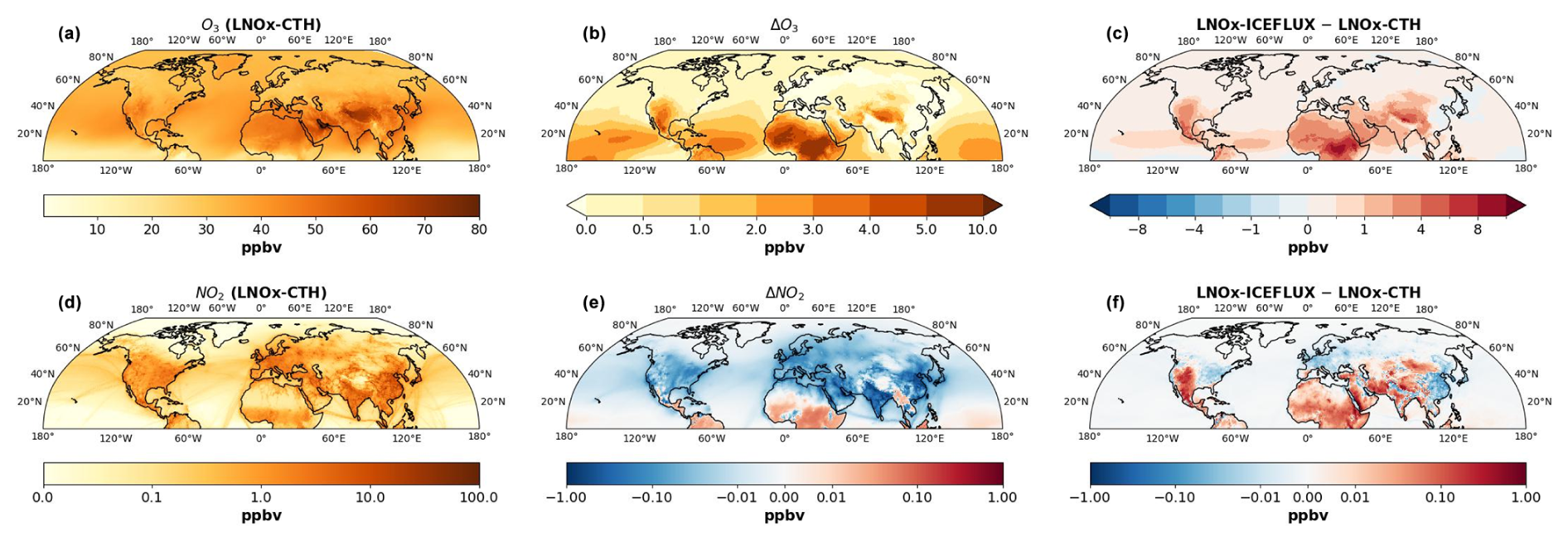
Figure 11 (a, d) Spatial distribution of annual mean mixing ratio (in ppbv) at the surface over the NH from experiment LNOx-CTH for (a) O₃ and (d) NO₂; (b, e) changes in mixing ratio at the surface due to inclusion of LNO_x emissions (LNOx-CTH − noLNOx) for (b) O₃ and (e) NO₂; (c, f) differences in mixing ratio at the surface from experiment LNOx-ICEFLUX with respect to LNOx-CTH for (c) O₃ and (f) NO₂; positive and negative values show an increase and decrease, respectively.

The statistical analyses are also done comparing the simulated mixing ratios at the surface to the observations and are presented in Table 6. The agreement between simulated and observed O₃ is considered good, as indicated by lower values of RMSE (10.7–11 ppbv), MAB (6.5–7.1 ppbv), and NME (26.9 %–27.8 %). In contrast, the comparison for simulated NO₂ with observations shows higher NME (51.5 %–52.7 %). Figure S7a–d represent the absolute bias in the simulated annual mean of O₃ and NO₂ at the surface from experiments LNOx-CTH and LNOx-ICEFLUX compared to the observations at available stations over the NH. The simulated O₃ and NO₂ mixing ratio is close enough to the observations at most of the stations over Europe and China, as well as over the USA for O₃ and Canada and South America for NO₂. A higher bias for O₃ is, nonetheless, observed over Canada, South America, and over eastern China. However, the inclusion of LNO_x does not significantly impact the statistical scores. A detailed analysis of the altitude-wise changes in the mixing ratio of O₃, due to the impact of LNO_x, is therefore necessary and has already been discussed in the Sect. 3.3.1 and 3.3.2.

3.5 Impacts on tropospheric OH burden and CH₄ lifetime

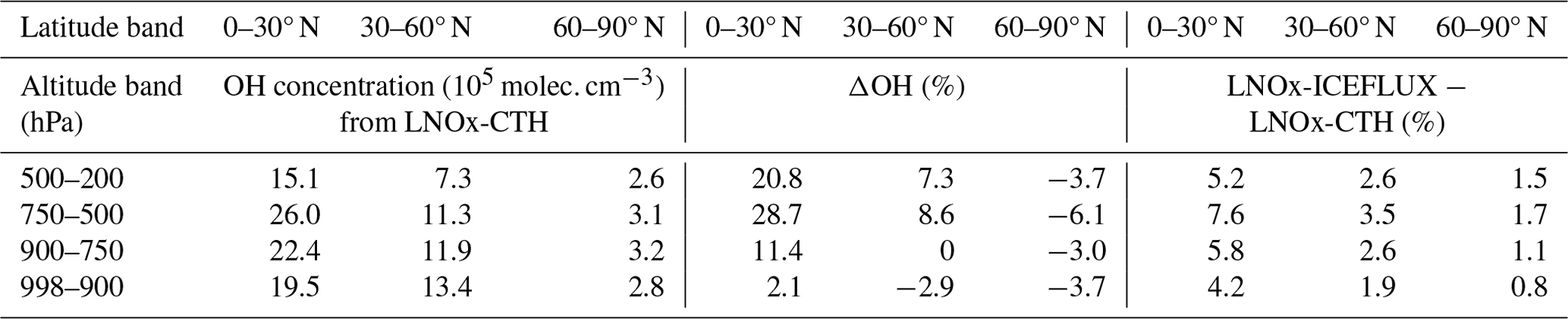
We also have evaluated the effects of LNO_x on tropospheric chemistry in terms of changes in the burden of a major oxidant (OH) and the lifetime of trace gas CH₄. Table 7 illustrates the concentration of OH from experiment LNOx-CTH and the changes in concentration of OH with respect to that from noLNOx averaged over selected latitude and altitude bands. The OH concentration from the LNOx-ICEFLUX is also compared with that from LNOx-CTH in Table 7. The OH concentration in our study, over the tropics, is almost twice higher and 6–7 times higher than that over mid-latitudes and polar regions, respectively, which is consistent with the study by Mao et al. (2021). Again these concentrations are close enough to those values obtained in a multi-model study by Naik et al. (2013) but shows a higher OH concentration in the tropical middle troposphere (22–26 × 10⁵ molec. cm⁻³), unlike the studies by Naik et al. (2013) and Luhar et al. (2021). A higher OH concentration in the upper troposphere is reported by Banerjee et al. (2014), due to transportation of water vapour through convection to the upper troposphere, promoting OH production due to reaction of exited state oxygen with water vapour. The annual mean OH concentration over the NH, from our study, is 14.5 × 10⁵ and 15.4 × 10⁵ molec. cm⁻³ from LNOx-CTH and LNOx-ICEFLUX, respectively, being 6.6 % and 13.2 % higher than that obtained from noLNOx simulation (Table 8). The annual mean OH concentration is higher by 30 %–38 % in comparison to the multi-model mean obtained from ACCMIP simulations (11.1 ± 1.8 × 10⁵ molec. cm⁻³; Naik et al., 2013; Voulgarakis et al., 2013). We find an increase in OH concentration due to LNO_x, which is again the largest over the free troposphere for the tropics (11 %–28 %), followed by mid-latitudes (Table 7). A 5 %–7 % higher OH concentration is also observed from LNOx-ICEFLUX in comparison to that from LNOx-CTH for the free troposphere. A warmer atmosphere for the tropics and high humidity favour the increase in OH and a faster OH to CH₄ reaction, causing a shorter CH₄ lifetime in these regions (Voulgarakis et al., 2013). The geographical distribution of changes in OH due to lightning is usually affected by the lightning parameterization used (Gordillo-Vázquez et al., 2019). The spatial distribution of changes in simulated OH concentration from LNOx-CTH with respect to noLNOx and from LNOx-ICEFLUX with respect to LNOx-CTH, at selected altitude bands, are also presented, respectively, in Figs. S8 and S9. The OH burden over the NH is increased by 14 % and 24 % in LNOx-CTH and LNOx-ICEFLUX, respectively, from 0.082 Gg, estimated in simulation noLNOx (Table 8).

Table 7 Analysis of simulated OH concentration averaged over selected latitude and altitude bands. ΔOH represents changes in OH from experiment LNOx-CTH with respect to that from experiment noLNOx; positive and negative values represent the increase and decrease in OH concentration, respectively.

In our study, we have estimated CH₄ lifetime (${\mathit{\tau }}_{{\text{CH}}_{\mathrm{4}}}$) due to chemical loss, mainly due to reaction with OH. The average lifetimes over the NH are 4.84 and 4.5 years, as obtained, respectively, from experiments LNOx-CTH and LNOx-ICEFLUX, which are reduced, respectively, by 11 % and 17 % compared to the estimate from the noLNOx simulation (Table 8). The CH₄ lifetime as estimated from previous modelling studies is within a range of 7–14 years (Naik et al., 2013; Lelieveld et al., 2016) and is visibly underestimated in our study. The CH₄ concentration is considered from chemical boundary conditions from the CAMS reanalysis dataset of atmospheric compositions produced by ECMWF, as in our study. CH₄ anthropogenic emissions are not taken into account. The annual mean CH₄ burden (1930–1933 Tg) estimated in this study over the NH is ∼ 20 % lower than the multi-model mean CH₄ burden, obtained from ACCMIP simulations (Naik et al., 2013), considering half of the global CH₄ burden over the NH (≈ 2406 Tg). As mentioned above, the OH concentration is also overestimated in our study. Therefore, the lower CH₄ burden and higher chemical loss due to reaction with OH cause the underestimated lifetime of CH₄ in this study, even in the absence of LNO_x. Therefore, the underestimated CH₄ lifetime in the present study is not attributed to LNO_x but likely stems from other factors including issues related to deficiencies in CH₄ burden, the chemistry, or photolysis schemes. Addressing and resolving these concerns will require further investigation in future studies. The CH₄ lifetime is underestimated, especially over the tropics, showing values of 2–4 years (Fig. S10). The lifetime increases with higher latitudes and is at a maximum at the polar region (40–60 years), which matches well with the estimated values from the study by Lelieveld et al. (2016) over higher latitudes (45–90° N).

Table 8 Tropospheric O₃, NO₂, OH burden, and CH₄ lifetime from simulation experiments. The numbers within parentheses represent the tropospheric O₃ burden over the domain from 0–60° N.

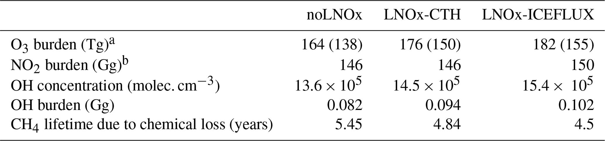
^a Tropospheric O₃ burden from OMI/MLS, estimated over the domain 0–60° N, is 159 Tg. ^b Tropospheric NO₂ burden over the NH from OMI is 164 Gg.

4 Conclusion

This study evaluates the incorporation of lightning-produced NO_x (LNO_x) into the CHIMERE chemistry–transport model to assess its impact on tropospheric ozone (O₃) over the Northern Hemisphere (NH). A classical lightning parameterization based on cloud-top height (CTH), developed by Price and Rind (1992), is applied (experiment: LNOx-CTH) with modifications to better align modelled flash rates over lands and oceans to satellite observations. Additionally, flash rates are computed using an updated ice-flux-based lightning scheme (experiment: LNOx-ICEFLUX; Finney et al., 2014). We perform a detailed evaluation of model simulations, integrating in situ measurements and satellite observations, to critically assess the reliability and applicability of these parameterizations. The annual flash frequencies over the NH are 20.7 and 21.6 flashes s⁻¹ as estimated from the LNOx-CTH and LNOx-ICEFLUX experiments, respectively. For LNOx-ICEFLUX, a correction factor of 5 is applied to the simulated annual flash frequencies. The estimated LNO_x emissions are 2.8 and 3.1 Tg N yr⁻¹ from the LNOx-CTH and LNOx-ICEFLUX experiments, respectively. Our study provides a comparative assessment of these two lightning parameterizations, evaluating their influence on modelled lightning flashes, LNO_x emissions, and tropospheric distribution of O₃ and trace gases, with implications for improving both the parameterizations and the model.

The major outcomes from our study are delineated here. Annual flash rates in tropical land and NH regions from both experiments, as well as in mid-latitudes from LNOx-ICEFLUX, show good agreement with satellite observations. Both the ICEFLUX and CTH schemes, as implemented in CHIMERE, reproduce the seasonal cycle of lightning flash rates correctly over the lands. LNO_x emissions peak during May–August, contributing 60 %–70 % to the total annual emissions, with most emissions concentrated in the tropics and mid-latitudes, and 60 %–65 % occurring in the mid-tropospheric region. The inclusion of LNO_x emissions in CHIMERE significantly improves the simulated tropospheric O₃ distribution, particularly in the free troposphere over the tropics. A significant bias at the upper troposphere and lower stratosphere at higher latitudes, however, highlights the necessity of improving the representation of stratosphere–troposphere exchange processes in the model. The model adequately simulates the O₃ and NO₂ burden over the NH compared to satellite observations, showing a 7 %–11 % increase in O₃ burden from 164 Tg, due to the inclusion LNO_x. Our study demonstrates that the inclusion of LNO_x consequently reduces the overall NO₂ column density over regions with high anthropogenic pollution. Additionally, it leads to a 14 %–24 % increase in OH burden from 0.082 Gg and an 11 %–17 % reduction in CH₄ lifetime compared to the without LNO_x scenario, though there remains scope for refining OH-related chemistry.

Our study underscores that, despite its simple representation, the CTH scheme better captures the spatial variability of flashes compared to satellite observations, outperforming the ICEFLUX scheme. However, the limitations of the CTH scheme in capturing mid-latitude flashes highlight the efficacy of the ICEFLUX scheme in these areas. Additionally, improving convective parameterization is crucial for better representation of oceanic flash rates. The ICEFLUX scheme also faces challenges in accurately simulating high-energy, less frequent flashes over oceans, emphasizing the need to incorporate additional factors alongside ice flux. The challenges to constrain parameters, such as cloud ice content and updraught mass flux, which are utilized in flux-based lightning schemes, continue due to limited available observations. A recent study by Cummings et al. (2024), which evaluated 18 lightning parameterization schemes, demonstrates that schemes based on storm kinematics and structure performed better than the microphysical schemes, in their study. Developing integrated parameterizations that incorporate both storm kinematics and microphysical processes, along with improved observational constraints, may provide a more robust and accurate representation of lightning flash rates, particularly in complex storm environments.