Monitoring of total and off-road NO_x emissions from Canadian oil sands surface mining using the Ozone Monitoring Instrument

The oil sands in Alberta, Canada, are a significant source of air pollution. Observations from the Ozone Monitoring Instrument (OMI) on the NASA Aura satellite have been used to quantify NO_x emissions from the surface mining region of the oil sands. Two related emissions methods were utilized, one for point and one for area sources, where OMI vertical column densities of NO₂ were combined with winds from a meteorological reanalysis and a two-dimensional exponentially modified Gaussian (EMG) plume model. This work better connects the two (point and area) emissions methods and discusses the interpretation of fit parameters and the ability of OMI (and other sensors) to resolve emissions between neighbouring sources.

The two methods employed, in good agreement with each other, indicated an increase in emissions from about 55 to 80 kt [NO₂] yr⁻¹ between 2005–2011 and a flat trend thereafter. Reported emissions were within 15 % of reported emissions, consistent to within uncertainties. In an extension of this methodology, OMI observations were combined with reported point source emissions to derive the more uncertain emissions component from the large off-road mining fleet. These were found to make up about 60 % of total NO_x emissions, also consistent with reported emissions. The OMI-derived 0.9 % yr⁻¹ increase in fleet emissions and the 5.5 % yr⁻¹ increase in bitumen mined, generally a good proxy for fleet emissions, can be reconciled by considering the evolution of the mine fleet over this period. OMI is therefore able to track the transition from US EPA Tier 1 standards, through Tier 4 standards, to the present and in doing so demonstrates the efficacy of this policy. Furthermore, this analysis shows that had the fleet remained at Tier 1, this source would currently be emitting an additional 40 kt [NO₂] yr⁻¹.

1 Introduction

The utilization of satellite observations of atmospheric composition for estimating or constraining emissions has expanded significantly in the past 2 decades (Streets et al., 2013) following improvements in sensor spatial resolution and precision, retrieval algorithms, and emissions methodologies. While satellite observations alone can often be used as proxies for emissions, at best they only contain information on the emitted mass of a pollutant and not the rate of emission. To bridge this divide, additional information on the dispersion (via atmospheric transport) and removal (though physical and chemical processes, if relevant) must be incorporated.

One common approach to obtaining “top-down” emissions estimates is through the use of 3D chemical transport or air quality models that simulate all relevant physical and chemical processes. Model emissions are adjusted such that the model-simulated and satellite-observed quantities match to within some tolerance. The specifics of the approach may depend on several factors such as resolution of the model and lifetime of the pollutant and vary from the straightforward mass balance (e.g. Martin et al., 2003) to a more formal Bayesian approach in which a cost function is minimized (Streets et al., 2013).

An alternative class of top-down methods have become increasingly common over the past decade in which satellite observations are paired with wind information to directly estimate emissions of air pollutants such as NO_x, SO₂, NH₃, CO, CH₄, and CO₂. This was done initially for point (or near-point) sources (Beirle et al., 2011; Pommier et al., 2013; Fioletov et al., 2015; Nassar et al., 2017; Varon et al., 2018; Dammers et al., 2019) but more recently for area sources (Fioletov et al., 2017; Beirle et al., 2019; McLinden et al., 2020; Fioletov et al., 2022; Liu et al., 2021; Wren et al., 2023; Fioletov et al., 2025). After several years of development, testing, refining, and validating, these methods are now being applied to emissions detection, verification, and analysis (e.g. McLinden et al., 2016b; Ialongo et al., 2018; Goldberg et al., 2019a; McLinden et al., 2020).

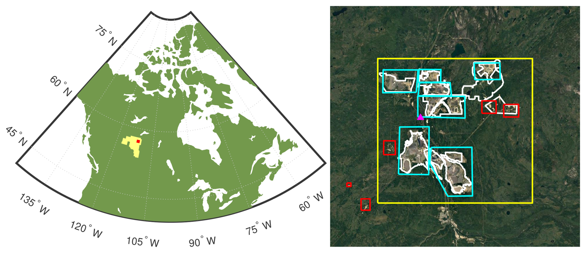
Figure 1 Left: map of the Canada showing the Athabasca oil sands region (yellow) and the location of the surface mining area (red), which also corresponds to the area outlined by the yellow box in the right panel. Right: map of the oil sands surface mining region (spanning 134 km N–S and 79 km E–W). The yellow box indicates the region over which emissions are added and assumed to be surface mining, although there are some minor emissions from in situ facilities that also reside within the yellow box. The cyan boxes indicate surface mines, whereas the red boxes are smaller in situ facilities. The magenta triangle shows the location of the Bertha Ganter – Fort McKay monitoring site, and the Fort Chipewyan site is 169 km due north of this. Map data: © Google, Image Landsat/Copernicus.

In this work, direct methodologies such as these have been applied to surface mining within the Athabasca Oil Sands Region (AOSR), located just north of the community of Fort McMurray (57° N, 111.6° W), in the Canadian province of Alberta (see Fig. 1). The AOSR contains large deposits of bitumen, a viscous form of oil, which can be converted into a synthetic crude oil. In total, the AOSR is estimated to contain the equivalent of 170 billion barrels of oil, making it the second-largest reserve globally. In 2023, production from the AOSR was (the equivalent of) 3.4 million barrels of oil per day (mBPD) from bitumen, a number expected to rise to 4.0 mBPD by 2030 (Alberta Energy Regulator, 2023b).

Within the AOSR, about 20 % of the proven reserves reside near the surface, at a depth of ∼ 75 m or less, and can be extracted through a process called surface mining. Surface mining first requires the removal of the overburden (muskeg and soil) in order to expose the deposit, followed by the extraction and transport of the raw bitumen to another on-site location for further processing to separate the bitumen from the sand and other impurities. For deeper deposits, in situ extraction methods must be employed in which steam is injected to reduce the bitumen viscosity so that it can be pumped to the surface. In either case, the bitumen is then converted into a synthetic crude oil through a process known as upgrading. Some facilities have on-site upgrading, while others transport the bitumen elsewhere.

There are a number of environmental concerns associated with oil sands operations (e.g. Kelly et al., 2010), including water usage; deforestation (Rosa et al., 2017); greenhouse gas emissions (Rosa et al., 2017; Liggio et al., 2019; Wren et al., 2023); and various potential environment effects to air, water, land, biota, and human health arising from the emission of pollutants, in particular, potential harmful effects on ecosystems from acidifying deposition (Makar et al., 2018), often referred to as cumulative effects. This refers to the environmental impact of past, present, and potentially future deposition, to the land and water. A comprehensive understanding of this impact, and how to mitigate it, requires an accurate knowledge of the emission rates of atmospheric pollutants (Galarneau et al., 2014; Gordon et al., 2015; Liggio et al., 2016; Li et al., 2017). Cumulative effects encompass many pollutants, but in this work the focus is nitrogen oxides, NO_x (or the sum of NO and NO₂), which are emitted as a by-product of combustion.

The Ozone Monitoring Instrument (OMI) satellite sensor has been used previously to help understand the distributions of NO₂ and SO₂ (McLinden et al., 2012, 2016a, 2020) in the AOSR. These studies showed that a “hotspot”, or local enhancement, in NO₂ can be readily observed over the surface mining. Likewise, OMI has been utilized to quantify NO_x emissions with methods similar to the method employed here from urban, industrial, and natural sources (Beirle et al., 2011; de Foy et al., 2014; Adams et al., 2019; Fioletov et al., 2022). This study builds on these to quantify NO_x emissions from AOSR surface mining using the now 19-year time series from OMI with the specific aim of understanding how they have evolved given its continued expansion and the changes in vehicle emissions standards over time.

2 Measurements and methods

2.1 Emissions data

This study is focused on quantifying NO_x emissions originating from a group of facilities within a region in the northeast corner of the AOSR dominated by surface mining, defined here by a box bounded by latitudes of 56.80 and 57.46° N and longitudes of 112.0 and 110.7° W. This box (see Figs. 1 and A1) contains all seven AOSR surface mining facilities, three relatively small in situ facilities, and other minor NO_x emitters such as the community of Fort McKay (pop. < 1000). Bottom-up inventories (Zhang et al., 2018) suggest that oil sands surface mining facilities and activities are responsible for roughly 95 % of total NO_x emissions within this area, and so the term “surface mining region” is used here for convenience. Just south of this area is the community of Fort McMurray (pop. 70 000, 15+ km south), and further south still are numerous in situ facilities (50+ km south).

Several sources of emissions information were used in this work. Annual emissions from point sources reported to the Canadian National Pollutant Release Inventory (NPRI) (Environment and Climate Change Canada, 2020) are available up to 2023. NPRI point source emissions are based on a variety of methods: some stacks employ continuous emissions monitoring systems (CEMS) (Alberta Government, 1998), others are based on engineering estimates, and some use a combination of both. The primary source of mine fleet emissions was created in accordance with the Environmental Protection and Enhancement Act (EPEA) (Alberta Environment and Parks, 2025) spanning 2010–2023, while those from the Cumulative Environmental Management Association (CEMA) for 2010 (Zhang et al., 2018) are also used for comparison. Related industrial activity data, including the total amount of oil sands mined on a monthly basis (Alberta Energy Regulator, 2023a), were helpful for interpretation and sampling corrections.

Emissions of NO_x from surface mining originate primarily from two source types. The first is the off-road vehicle fleet composed of large, diesel shovels and trucks that operate $\mathrm{24}/\mathrm{7}$. Three of the seven mining operations also have large point sources, stack emissions, from the upgraders that convert the bitumen into a synthetic crude oil. The in situ facilities also have stack emissions, though these are quite modest (< 5 %) in comparison. The databases indicate that, in 2010, within the surface mining region, roughly 38 kt [NO₂ yr⁻¹] originated from the surface mining off-road fleet, 29 kt [NO₂ yr⁻¹] from surface mine point sources, and about 1–2 kt [NO₂ yr⁻¹] from in situ point sources. All other sources are estimated to emit considerably less than 1 kt [NO₂ yr⁻¹] and are therefore ignored.

2.2 OMI observations

OMI is a Dutch–Finnish instrument launched in 2004 on the NASA Aura satellite (Levelt et al., 2006, 2018). OMI measures back-scattered sunlight in the UV–visible using a two-dimensional detector that measures simultaneously at 60 across-track positions. Its spatial resolution at nadir is 13 × 24 km², but it gets progressively worse at larger off-nadir angles. A blockage beginning in 2007 – the so-called “row anomaly” – has meant some track positions are no longer reliable (Levelt et al., 2018; van Geffen et al., 2020). As of 2023, more than half of the across-track positions were affected.

Version 4.0 of the OMI NO₂ standard product (Krotkov et al., 2024; Lamsal et al., 2021) is used here. It, like many UV–visible NO₂ retrievals, uses a three-step approach to determine tropospheric NO₂ vertical column densities (VCDs) from measured spectra, where the tropospheric VCD represents the vertically integrated number density between the surface and the tropopause.

The first step in the retrieval is a determination of the total absorption by NO₂, quantified in terms of a slant column density (SCD). The SCD represents the NO₂ number density integrated along the path of the sunlight through the atmosphere. Since OMI measures scattered light, the path is complex and includes one or more scattering events and/or surface reflections. SCDs are derived through an analysis of the measured spectra by exploiting the difference in absorption at nearby wavelengths and involves a spectral fit of reference spectra, one of which is the NO₂ absorption cross-sections, to the measured spectra . The second step is the removal of the stratospheric component of the total SCD. This is accomplished using a complex high-pass filtering approach. The final step is a conversion of the remaining tropospheric SCD into a tropospheric VCD via an air mass factor (AMF) that accounts for the sensitivity of the instrument to NO₂ for a particular scene, where VCD = SCD $/$ AMF. In practical terms, a multiple-scattering model is used to calculate AMFs (Palmer et al., 2001) to account for the complex path of light through the atmosphere. AMFs depend on factors such as solar and viewing geometry, the presence of clouds, scene reflectivity, and the vertical distribution of NO₂.

AMFs are one of the largest sources of uncertainty in NO₂ VCDs (Lorente et al., 2017). In the OMI NO₂ standard product (SP, version 4.0), model profiles at 1° resolution are used for the vertical distribution. As these are coarser than the individual OMI pixels, this acts to smooth the VCD distribution. To improve the effective spatial resolution, AMFs were recalculated using higher-resolution inputs and more recent oil sands emissions (McLinden et al., 2014). These inputs include NO₂ profiles from the Global Environmental Multi-scale – Modelling Air quality and CHemistry (GEM-MACH) forecast model, discussed in Sect. 2.3, and an annually varying monthly-mean MODIS clear-sky reflectivity at 0.05° (Schaaf et al., 2002) smoothed to 15 km. Furthermore, snow pixels are identified using the Interactive Multisensor Snow and Ice Mapping System (Helfrich et al., 2007), which was found to be the snow product best suited for distinguishing between snow-free and snow-covered scenes (Cooper et al., 2018). When snow was detected, AMFs were then calculated using a MODIS-derived 15 km snow reflectivity as per McLinden et al. (2014).

OMI NO₂ VCDs were filtered as follows: track positions affected by the row anomaly are not used, and the track positions at the edge of the detector, 1–7 and 54–60, which correspond to the coarsest spatial resolution, are also removed. Note that pixels affected by the row anomaly change over the course of the mission, which impacts both the data density and, as discussed below in Fig. 3c, the effective spatial resolution. See Torres et al. (2018) for more information on the evolution of the row anomaly. Only observations made for solar zenith angles (SZAs) of 75° or less are retained. At a latitude of 57° N, this removes the majority of data for the months of November to January. Note that a seasonal correction was developed to account for this in the determination of annual emissions (see Sect. 2.4.4, below).

2.3 The GEM-MACH air quality forecast model

This study utilizes output from the Canadian Global Environmental Multi-scale – Modelling air quality and Chemistry (GEM-MACH) regional operational air quality forecast model (Moran et al., 2010; Pavlovic et al., 2016; Makar et al., 2017; Pendlebury et al., 2018), which covers most of North America. GEM-MACH is an online chemical transport module that is embedded within the ECCC weather forecast model. GEM-MACH was utilized as described in McLinden et al. (2014) where monthly-mean NO₂ profiles at 15 km × 15 km were computed for use in the AMF calculations. As discussed below in Sect. 2.4.3, GEM-MACH was also used to better quantify the NO₂ $/$ NO_x ratio.

2.4 Satellite-derived emissions

Emissions are derived using a direct approach in which wind information is paired with individual OMI NO₂ VCD observations. In this step, vertical profiles of the u and v components of wind speed are obtained from the ECMWF (European Centre for Medium-Range Weather Forecasts) reanalyses, ERA-5 (Hersbach et al., 2020).

From here, two related emission algorithms are employed: one developed for isolated, near-point sources (Fioletov et al., 2015) and one for multiple or area sources (Fioletov et al., 2017). Both algorithms rely on a two-dimensional exponentially modified Gaussian (EMG) plume function, which translates the emissions into a spatial distribution. The functional form for the 2D EMG, provided in Appendix B, is essentially a modified version of the traditional Gaussian plume with simple (e-fold) chemistry (Stockie, 2011) but is integrated in the vertical dimension and accounts for the finite size of the source and spatial resolution of the instrument. The EMG plume distribution varies with upwind/downwind and across-wind distance from a reference point that represents the location of the source and wind speed and also depends on three parameters: pollutant mass, m; its effective lifetime τ; and a plume width parameter, σ. The emission rate, assuming a mass balance, is simply $E=m/\mathit{\tau }$. Henceforth the EMG will be described as a function of (E, τ, σ) for simplicity.

The effective lifetime describes the rate of decay of the pollutant due to chemical (e.g. conversion into other species) or physical (e.g. dry deposition) loss. It is well known that the lifetime of NO_x depends on NO_x itself, and a recent study (Laughner and Cohen, 2019) elucidates this in the context of theoretical NO_x-lifetime curves for various volatile organic compound reactivity regimes. Previous studies using EMG-like functions found effective lifetimes of 2–5 h by following the downwind decay of NO₂ VCDs (Beirle et al., 2011; de Foy et al., 2015; Lange et al., 2022).

The effective plume width (or spread) parameter, σ, is interpreted as a combination of a plume diffusion parameter, σ_diff, the spatial resolution of the satellite instrument, σ_pixel, and the physical size or extent or size of the source itself, σ_size. Given the Gaussian nature of the EMG, it is reasonable to assume that these are related through a functional form resembling

$$\begin{array}{}\text{(1)}& {\mathit{\sigma }}^{\mathrm{2}}={\mathit{\sigma }}_{\mathrm{diff}}^{\mathrm{2}}+{\mathit{\sigma }}_{\mathrm{pixel}}^{\mathrm{2}}+{\mathit{\sigma }}_{\mathrm{size}}^{\mathrm{2}}.\end{array}$$

Considering the physical extent of the oil sands, σ_size is expected to be tens of kilometres. Similarly, given the OMI spatial resolution, σ_pixel should be on the order of 20 km. The remaining term, from Eq. (B4), is ${\mathit{\sigma }}_{\mathrm{diff}}^{\mathrm{2}}=\mathit{\alpha }\cdot y^{\mathit{\beta }}$, where y is the downwind distance, and α=1.5 km and β=1 (Fioletov et al., 2015). Conventional Gaussian plume models use values more like α=0.33 km and β=0.86 (Stockie, 2011). The larger value for α accounts for additional uncertainty in the wind downwind of the source. In the case of OMI, with its rather coarse resolution, decreasing α has virtually no impact on the fit.

The precise relationship between σ, σ_diff, σ_size, and σ_pixel is explored in Appendix F using a simple model in which a collection of true Gaussian plume point sources were used to simulate a near-point source (of some radius σ_size) and smoothed to a specified satellite resolution (for pixel size σ_pixel). Fitting this combined distribution to an EMG allowed a relationship between these various terms to be established. Figure F1 shows σ has a dependence reminiscent of ${\mathit{\sigma }}_{\mathrm{size}}^{\mathrm{2}}$ and ${\mathit{\sigma }}_{\mathrm{pixel}}^{\mathrm{2}}$ and, for small values of both, values less than 1 km, which suggests σ_diff is small. Figure F1 will be used below to help interpret results. This further suggests that only for instruments with substantially higher spatial resolution than OMI, and likely even TROPOMI or TEMPO (Zoogman et al., 2017), would this σ_diff term need to be refined.

The EMG plume function is used in two ways. The first is an inverse mode, where combined OMI-wind data are fit in order to derive (E, τ, σ). The second way is in a forward mode to predict the spatial distribution of VCDs (at an OMI-like spatial resolution) by prescribing winds and values for (E, τ, σ). The input emissions used for this forward mode can be those derived from OMI (in the inverse mode), in which case the intent is to “reconstruct” the original OMI observations to test for consistency. Alternatively, a modified or even completely independent source of emissions, E, can be used, with τ and σ as derived from OMI, in order to examine the predicted spatial distribution of VCD (at OMI spatial resolution).

2.4.1 Point source method

The first emissions approach considered is the point source method of Fioletov et al. (2015), used previously to derive emissions of SO₂ (Fioletov et al., 2016; McLinden et al., 2020), NH₃ (Dammers et al., 2019), and NO_x (Griffin et al., 2021). Observations from many OMI overpasses are combined using a rotation procedure in which all observations are re-positioned about a reference location according to their individual wind directions such that, after rotation, all observations share a common wind direction (Pommier et al., 2013). In other words, the upwind/downwind and cross-wind positions, relative to the reference location, of each observation are preserved. In this way multiple overpasses can be analyzed as a single, average plume. In this method values of (E, τ, σ) are determined that minimize the difference between the EMG plume function and the OMI observations in the rotated plume. Since τ and σ are non-linear parameters, a non-linear solver is used. A variation of this method is also used in which τ and σ are prescribed, thereby allowing E to be determined using a linear regression, which is more stable and often means fewer observations are required. Details on the practical implementation of this method are given in Appendix C.

2.4.2 Multi-source method

The second method, developed for multiple or area sources (Fioletov et al., 2017, 2022), was also employed. This is a complementary approach to the point source method in that the same EMG plume function is used except here (τ, σ) specified and emissions from multiple locations are solved for simultaneously. At each location, an EMG basis function is generated for all OMI observations being used in the fit. The OMI VCDs are modelled as the sum of all EMG functions which represent the local sources, and a background term, which represent the NO₂ that would be present in the absence of local sources. The background can be a simple constant offset or allowed to vary linearly in latitude and longitude. A multi-linear regression is then performed which provides a set of emissions that minimize the difference between the OMI and modelled (or reconstructed) VCDs. Unlike the point source method, this fit is performed in the original latitude–longitude frame (i.e. not in the rotated frame) and a positive constraint is placed on the emissions.

In this multi-source method, the choice of emission locations is arbitrary. If the emission sources are well known, then these locations can be used. Likewise, a grid of locations can be used when their spatial distribution is uncertain or complex. One aspect of this approach is that τ and σ must be specified. While the effective lifetime can be estimated from a model, there is a question as to how precisely to do this. An alternative approach, and the one adopted here, is to use the effective lifetime derived from the point source method. The choice of σ is not necessarily obvious since it encompasses multiple parameters, as indicated by Eq. (1). It should be chosen such that σ_size represents the physical size of the emissions. For a collection of point sources, σ_size=0. For a grid representing an area source, σ_size should be on par with the grid spacing. Of course, this assumes σ_OMI, or at least ${\mathit{\sigma }}_{\mathrm{diff}}^{\mathrm{2}}+{\mathit{\sigma }}_{\mathrm{OMI}}^{\mathrm{2}}$, is known. One method to estimate these other terms is to fit σ for a true point source, as is discussed below. Additional information is provided in Appendix D.

2.4.3 Other considerations

One important parameter that must be specified is the altitude of the winds, where the altitude is chosen to represent the average height of the NO₂ plumes. As emissions are roughly proportional to wind speed, and wind speeds typically increase rapidly with height through the boundary layer, this also represents one of the larger sources of uncertainties. Previous studies used winds averaged over the lowest 500 m for urban, primarily vehicle (Goldberg et al., 2019a), emissions, while another study used winds over the lowest 1 km (Fioletov et al., 2015).

In this work, wind heights are based on the observations from aircraft campaigns conducted in 2013 and 2018 which studied pollutant transformation downwind of the oil sands (Li et al., 2017; Liggio et al., 2019). These aircraft data indicated that NO_x within plumes was found to reside at altitudes between the lowest altitudes sampled by the aircraft (100–300 m above the surface) and 800 m. In these same plumes, SO₂, which originates only from the upgrader stacks (e.g. McLinden et al., 2020), was found at 400–800 m. This indicates that NO_x from the upgrader stacks is best represented at 400–800 m while emissions from the fleet at 0–400 m. On this basis, and assuming roughly equal emissions from the stacks and the vehicles as suggested by the bottom-up inventory, winds, averaged between the surface and 800 m, will be used for the majority of the analysis herein. Furthermore, an uncertainty of 100 m is assigned to the wind height, which translates into a difference in wind speed of roughly 10 % since, in the vicinity of the oil sands, wind speeds on average were found to roughly double between the surface and 1000 m. For situations where fleet and stack emissions are treated separately, winds averaged over 0–400 and 400–800 m are used, respectively.

As OMI only observes NO₂ a correction must be applied to account for the missing NO. Typically this is done by estimating the NO_x $/$ NO₂ concentration ratio and scaling the derived emissions by this. Previous studies often used more generic values of 1.3–1.4 (Beirle et al., 2011; Goldberg et al., 2019a). Here, a site-specific value was determined from the GEM-MACH model. The annual average surface mining concentration ratio for NO_x $/$ NO₂, considering grid boxes within a 40 km radius and using the same monthly sampling pattern as OMI, is 1.50. The larger value is due in part to the inclusion of non-summertime chemistry where the photolysis of NO₂ is typically slower, particularly at higher latitudes.

However, using a single concentration ratio does not account for any spatial variability. Close to the actual site of the emissions this ratio can be larger as NO_x is primarily emitted as NO (relatively less NO_x is NO₂), while further downwind the opposite is true (relatively more NO_x present as NO₂). This acts to skew the shape of the (rotated) plume thereby impacting the fit. Similar to Griffin et al. (2021), the GEM-MACH model is used to quantify the impact of this: VCDs of NO₂ and NO_x for a year of simulations over the oil sands, along with model winds, are each fit to the EMG plume function using the point source method. Taking the ratio of NO_x to NO₂ emissions derived in this way reveals a ratio of 1.63, which is roughly 10 % higher than the simple concentration ratio. This 10 % difference is a systematic effect that should be largely independent of location provided emissions are from combustion. This value of 1.63 was used here. See Appendix F for additional information.

2.4.4 Uncertainties

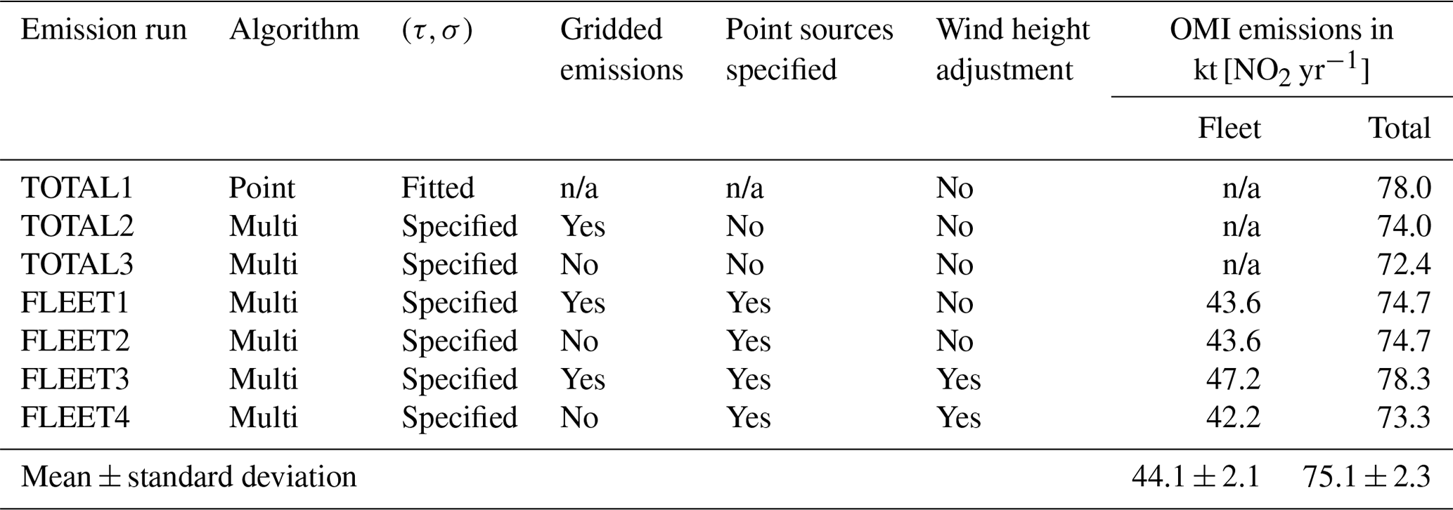
There are several sources of uncertainty that limit the accuracy and precision of these OMI-derived emissions. Table 1 shows a breakdown, with each listed as a random or systematic sources of uncertainty, for the point source method. They are arranged under five categories – AMF, data filtering, the EMG fit, winds, and the NO_x $/$ NO₂ ratio.

Table 1 OMI NO_x emissions uncertainty budget when considering 3 years of observations. For the uncertainty type, R is random, and S is systematic.

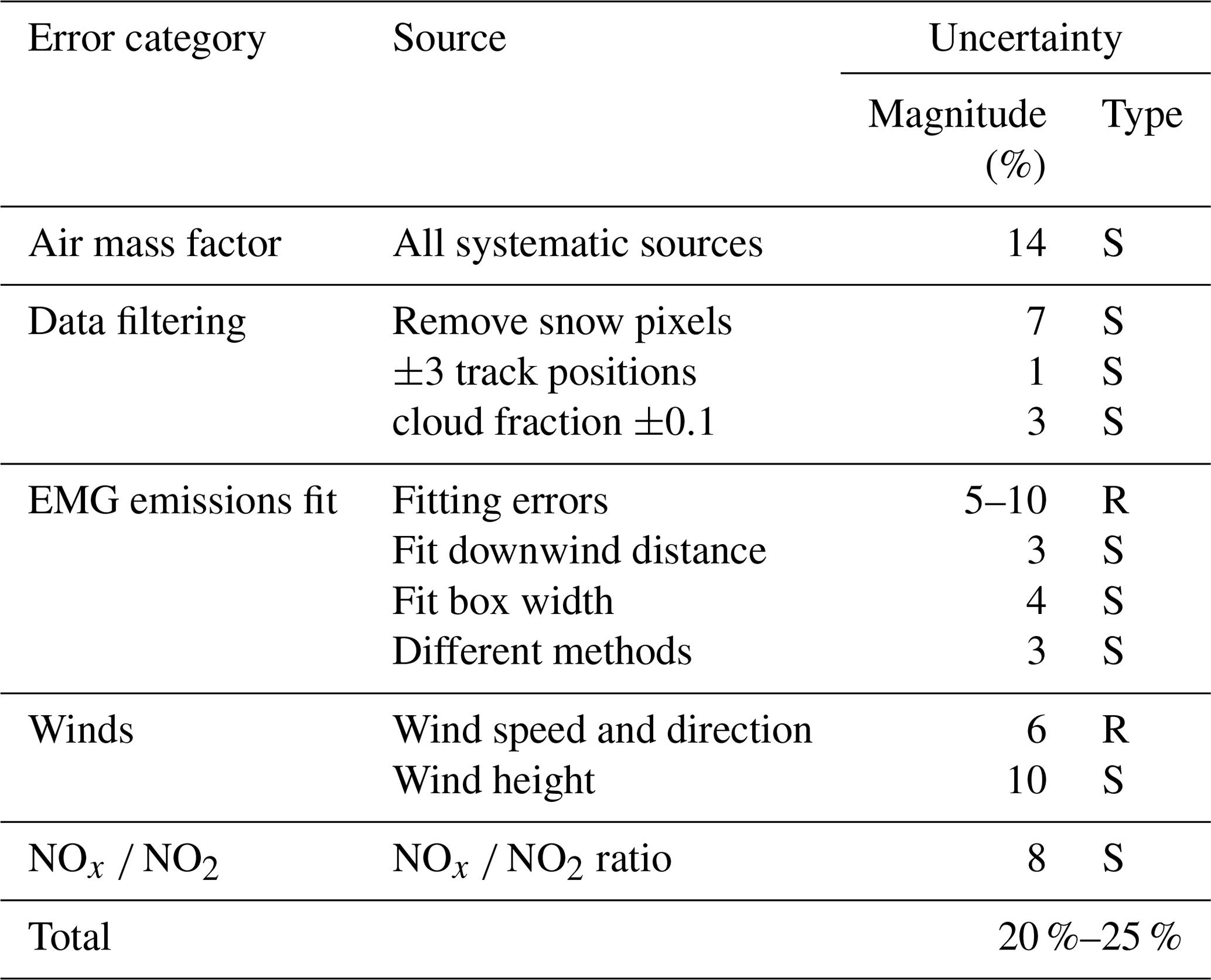
Only systematic errors in AMFs are considered since random errors should largely cancel out as data spanning multiple years are analyzed together. A previous study (McLinden et al., 2014) found systematic uncertainties to be 14 % due to approximations with how aerosols are handled and the use of a Lambertian surface albedo. Data filtering refers to what OMI data are included or excluded in the analysis for which different thresholds could be argued: exclusion of snow pixels; track position cut-off, which really denotes the maximum size of the pixels; and maximum cloud fraction. These are systematic effects that collectively represent an 8 % uncertainty.

The EMG fit contributes a random uncertainty to emissions related to the quality of the fit itself, which varies from 5 %–10 % depending on the number of data used. Beyond that, there are small systematic effects when it comes to the spatial domain used in the fit itself, specifically the cross-wind, upwind, and downwind distances. There is also a small uncertainty included here that reflects how different variants of the algorithm produce slightly different emissions.

From Sect. 2.4.3, a systematic error of 10 % from using an incorrect wind height is reasonable. Also, random errors in wind speed and direction were estimated to be 6 % from a previous study (McLinden et al., 2016b). The NO_x $/$ NO₂ emission ratio used here is 1.63 as discussed in Sect. 2.4.3. An 8 % systematic uncertainty is assigned to this category, arrived at by considering the differences between the average of the aircraft measurements from Fig. E3 and multiple years of GEM-MACH output.

There are also potential sources of bias due to the sampling of the OMI instrument: overpasses are only in the early afternoon, and there is an unequal distribution of observations throughout the year. The first of these is only an issue if there is a diurnal cycle in emissions. Hourly emissions of SO₂, co-emitted with NO_x, from the upgraders indicate no consistent difference in time of day emissions. Likewise, the heavy-hauler fleet of trucks is used $\mathrm{24}/\mathrm{7}$, and it is assumed there is no systematic diurnal variation in these emissions. High-resolution GEM-MACH forecasts assume flat NO_x emissions for both source types (Zhang et al., 2018). In addition, the fitting algorithm itself smooths the diurnal cycle impact to some extent as NO_x emitted before the overpass time is sampled downwind.

Any potential seasonality bias is largely eliminated using OMI observations from all months. Nonetheless, the SZA cut-off of 75° and the change in cloud cover with season means not all months contribute equally. The impact of this is assessed using monthly bitumen mining data (Alberta Energy Regulator, 2023a). Each OMI pixel is assigned a bitumen-mined value equal to its corresponding monthly total. An annual average bitumen-mined value was then calculated averaging over all pixel values, thereby capturing the OMI sampling, and these were then compared to the average assuming an equal weighting. The resultant bias is typically about 1 %–2 %, with 1 year reaching 5 %. This correction was applied directly to the OMI emissions. See Appendix F for the time series and additional information.

Constructing an error budget for the multi-source method is more challenging, but it is argued here that it would be very similar since the largest contributors are systematic errors from the AMFs and winds, which would be common to both. As discussed below, fitted parameters from the point source method are used as inputs to the multi-source which also speaks to their connection. Given all this, and what was found to be a high degree of consistency in emissions as obtained from each method, this uncertainty budget is used for both approaches.

It is worth noting that the uncertainties derived here are smaller than those reported in other satellite-based NO_x emission studies. There are several reasons for this: (i) location-specific and temporally resolved fitting parameters (τ and σ), (ii) the use of multiple years of data to reduce fit uncertainties, (iii) aircraft observations of real plumes providing more confidence in wind heights, and (iv) a location-specific and more detailed consideration of the NO₂ $/$ NO_x ratio.

3 NO_x emissions from the oil sands

3.1 Surface mining as a point source

An initial assessment of NO_x emissions for oil sands surface mining is made using the point source method. Here, a reference location of 55.06° N, 111.55° W is used as it is the location of the maximum in the mean OMI NO₂ VCD distribution, as shown in Fig. 2a. Winds are taken as the average between the surface and 800 m (see Sect. 2.4.3). Figure 2 shows a summary of the emissions procedure considering the entire OMI time series (2005–2024). These maps were created using a 2 × 2 km² grid and a 12 km oversampling radius (Fioletov et al., 2011). Figure 2a shows the mean NO₂ VCD along with an outline of the surface mines and the reference location. Figure 2b uses the same data as Fig. 2a but averaged in the rotated frame, as a function of downwind and cross-wind distance from the reference location. In this frame the reference location corresponds to (0,0). There is a clear plume-like feature that peaks just downwind of the reference location before it decays close to background some 100–150 km downwind. The peak value in the rotated frame is roughly 10 %–15 % larger as compared to the original frame as a result of a greater cohesion in the distribution. Figure 2d shows the map that results from the non-linear fit of the individual VCD observations to the EMG plume function in the rotated frame, and it can be seem to capture the shape of the average plume in Fig. 2b. The fit parameters are $E=\mathrm{69.7}\pm \mathrm{2.2}$ kt [NO₂] yr⁻¹, $\mathit{\tau }=\mathrm{3.2}\pm \mathrm{0.1}$ h, and $\mathit{\sigma }=\mathrm{20.6}\pm \mathrm{0.3}$ km, where the uncertainties are statistical only, an indication of how well the EMG represents the OMI/wind observations. The overall uncertainty in the emissions would be roughly ±20 %, from Sect. 2.4.4.

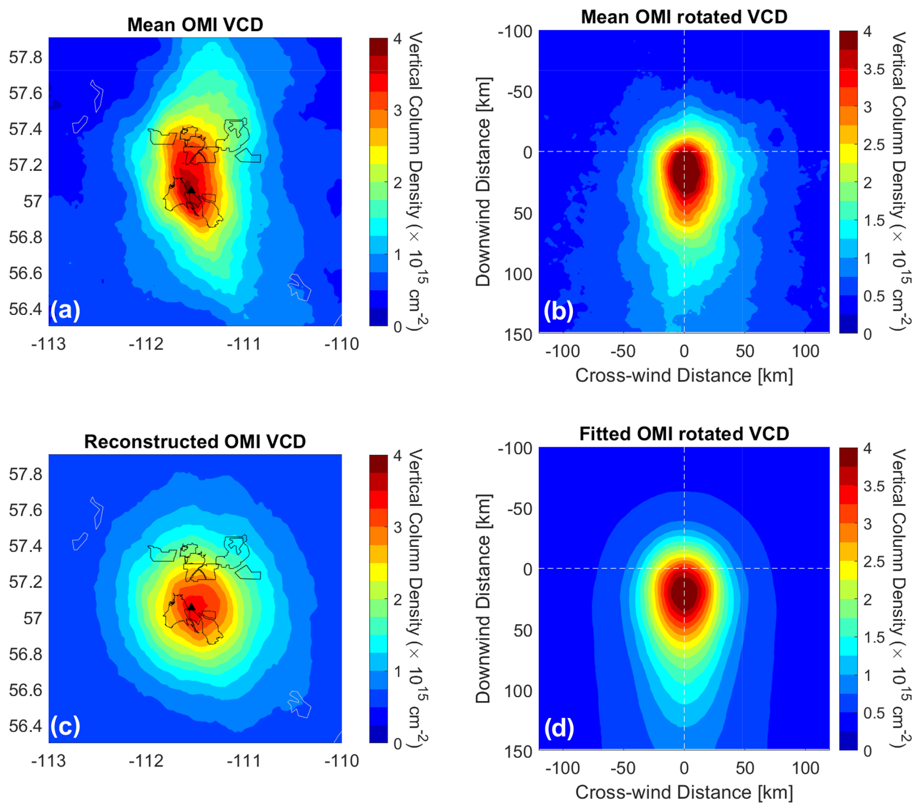
Figure 2 Summary of the point source emissions procedure using 2005–2022 OMI NO₂ VCDs. (a) Mean OMI VCD over the surface mining region of the oil sands. The black lines denote the different mining operations; (b) mean OMI VCD after rotation showing plume-like structure; (c) reconstructed spatial distribution using EMG plume and fitted parameters; (d) fit to rotated VCD using 2D EMG plume function, with fitted parameters of E=69.7 kt [NO₂] yr⁻¹, τ=3.2 h, and σ=20.6 km. The black triangles in panels (a) and (c) show the reference location used in the emissions retrieval that corresponds to the (0,0) point in panels (b) and (d).

The remaining panel, Fig. 2c, shows the reconstructed VCD distribution as found by rotating the fitted values in Fig. 2d back to the original latitude–longitude co-ordinates. This generally resembles the mean OMI VCD map in Fig. 2a but has a smaller peak value and appears much more symmetric. This is a result of assuming all emissions originate from a single point, the reference location given by the triangle. Of course in reality emissions are spread out (see Fig. 1) over a 60 km (N–S) × 40 km (E–W) expanse, which motivates the use of the area or multi-source approach. The only reason why the reconstruction from Fig. 2c departs from a symmetrical pattern is that there is a preferred wind direction, out of the W and SW.

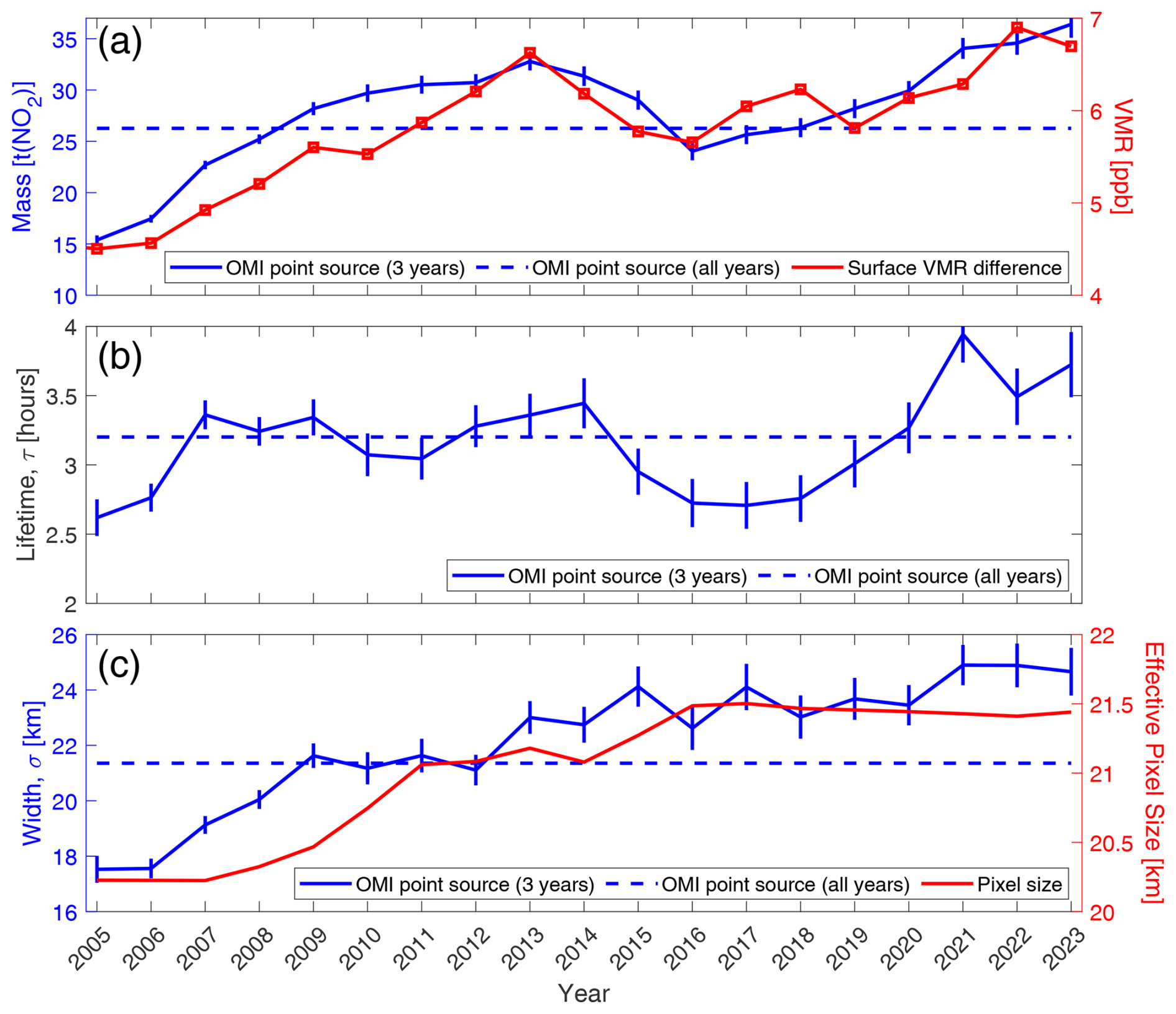
Figure 3 OMI point source emissions and parameter time series: (a) mass of the NO₂ enhancement and, for comparison, the difference in surface volume mixing ratio (VMR) between a surface mining and background site (see text); (b) effective lifetime of plume; and (c) plume width parameter and effective OMI pixel size, calculated as the square root of the mean of pixel area. All OMI-derived quantities are based on 3 years of observations, such that, for example, 2006 considered observations from 2005–2007, with the exception of 2005, which is based on 2 years, 2005–2006.

This approach is repeated but now considering successive 3-year time periods, where 3 years is combined to help ensure the stability of the non-linear, fitted parameters τ and σ, particularly in latter years when the row anomaly means less than half of all pixels are usable. An example of the mean and fitted VCD plots, analogous to Fig. 2 but for 2005–2007, is given in Fig. C1. The fitted parameters are presented first, deferring any discussion of the emissions to Sect. 2.4. Figure 3a shows the time series of the mass of the NO₂ enhancement. This represents the average mass of NO₂ that is present as a consequence of the surface mining NO_x emissions discussed in Sect. 2.4. It is seen to increase with time, peaking mid-time series (∼ 2013) and then decreasing slightly. The dip in 2016 is attributed to the large forest fire just south of the surface mining in and around the community of Fort McMurray (Adams et al., 2019) that significantly impacted production throughout the month of May. Note that NO_x from the fires themselves originated 20 km south of the surface mines and 2 weeks later approached the southernmost edge (MNP, 2017). There is only 1 or 2 d for which it is conceivable that there could be some misidentification of fire NO_x for oil sands, but given their proximity and wind direction, these data tended to be filtered due to a higher cloud fraction. There is no obvious sign that COVID-19 public health restrictions affected emissions in the most recent years, consistent with the 2020–2023 production data remaining roughly constant compared with previous years (Alberta Energy Regulator, 2023b). The increase in the 1σ fitting error bars (in all panels, Fig. 3a–c) reflects the decrease in the number of OMI pixels due to the onset and expansion of the row anomaly.

For comparison, the 3-year running average of in situ NO₂ volume mixing ratio (VMR) is also shown in Fig. 3a. Here, the average from the Bertha Ganter – Fort McKay monitoring station, located between the northern and southern cluster of mines, is used but, subtracted from it, is the NO₂ from a background station at Fort Chipewyan, roughly 170 km to the north. This difference in station values is used as the mass reflects an enhancement in NO₂ above background levels due to the local sources. While this simple comparison cannot be considered a validation, their general consistency provides confidence in the approach.

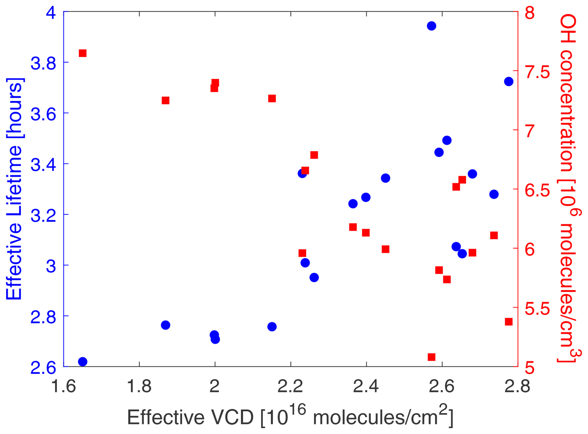
From Fig. 3b, the effective lifetime displays some variation with time, between 2.7–3.9 h. It is well known than NO₂ can impact the abundance of OH, and hence its own lifetime (Valin et al., 2013), and it is in this context that this is explored further, below. Krol et al. (2024) also highlight the importance of not using a single lifetime for an accurate determination of emissions.

The variation of σ is shown in Fig. 3c, where it is seen to increase from ∼ 18 km in the mid-2000s to ∼ 21 km by 2009 and with a smaller rate of increase to ∼ 24 km near the end of the OMI record. This is broadly consistent with an expansion of the surface mining activities in the north, including new mining operations coming online, which effectively increase the area of NO_x emissions. Also shown is the average effective size of the OMI pixels used in the analysis, calculated here as the square root of mean pixel area, and it is seen to increase slightly with time due to the expansion of the row anomaly, particularly through 2008–2011. While similar to the increase in σ, the magnitude of the increase in pixel size is much smaller. The link between pixel size and σ is discussed below. From Fig. F1, 21 km pixels for a surface mining radius of 30 km would predict a value for σ of about 21 km, consistent with that derived here.

These results can be contrasted with a previous study (McLinden et al., 2012) in which, between 2005–2011, the mass was seen to increase at a similar rate over this period but was a factor of 2–3 smaller. This is due primarily to the differences in AMF, where the former study used the VCDs as provided in the KNMI version 2 data product (Boersma et al., 2011). In that data product, the model-simulated NO₂ profiles were for background conditions as it has no emissions in the AOSR (McLinden et al., 2014). Other differences are due to the data version and the more sophisticated fitting in this work. It is this difference in fitting that also complicates any quantitative comparison between the fitted width parameters in these two studies.

In order to examine the variation in lifetime more thoroughly, an effective-VCD was derived using the mass from Fig. 3a (converted to molecules) and divided by an area taken to be $\mathit{\pi }{\mathit{\sigma }}_{\mathrm{eff}}^{\mathrm{2}}$, where σ_eff is the width parameter from Fig. 3c. This would peak at the middle and end of the time series and be a minimum towards the early years. Note that such a quantity is not the mean VCD but simply one that accounts for the changing spatial extent of the source with time. Plotting this effective lifetime vs. effective VCD shows a reasonably compact relationship, as shown in Fig. 4, with a correlation coefficient of 0.78. For pure chemical loss of NO_x via NO₂ + OH, $\left[\mathrm{OH}\right]=\mathrm{1}/(k_{\mathrm{OH}+{\mathrm{NO}}_{\mathrm{2}}}\cdot \mathit{\tau })$ can be used to estimate [OH], giving values between 5–8 × 10⁶ molec. cm⁻³, also shown in Fig. 4. For the 2013 flight campaign in the oil sands, summertime OH was estimated at 10 × 10⁶ molec. cm⁻³ (Liggio et al., 2016). The 2013 value from this OMI analysis, 6 × 10⁶ molec. cm⁻³, is generally consistent since it considers all seasons (albeit weighted towards spring and summer), and wintertime values would be considerably smaller. This analysis suggests that at least some of the temporal variation of τ is real and highlights the importance of using the period-specific τ when estimating emissions. Using the 2005–2023 mean τ (or some other constant value) could lead to a 10 %–15 % additional error and skew the trend.

Figure 4 Relationship between effective VCD and lifetime and inferred OH concentration. Each point represents one 3-year value from Fig. 3.

3.2 Surface mining as a collection of point sources

When quantifying emissions from a location where the spatial scale of the emissions is larger than σ (as is the case here), the multi-source method may be more appropriate than the point source method. If the locations of the emissions are well known, then these can simply be specified; alternatively, a grid of potential source locations can be used. In this work both options were explored.

Initially, a grid of potential source locations covering the entire surface mining region is used. Initially an 8 × 8 km² grid is defined over an area of 250 km × 250 km centred on the surface mining. Each grid box is treated as a (potential) point source, analogous to the approach used in Fioletov et al. (2017). As discussed in Sect. 2.4 and Appendix D, emissions are derived for each grid box such that their combined VCDs match the OMI observations. The positive constraint ensures most of these fitted values, and hence emissions, are zero.

In this approach σ and τ must be specified. Here τ is taken from the point source analysis in Fig. 3b and used for all individual sources. This is a simplification as it was already demonstrated in Fig. 4 that τ depends on VCD and hence local emissions. It is argued here that this will be a secondary effect since (i) plumes from individual sources will frequently overlap due their proximity and the coarse spatial resolution of OMI and (ii) significant cancellation of errors since the point source lifetime used was for the combination of all local sources, small and large. In the future, when isolating individual sources is the goal, it would be worthwhile exploring a parametrization which might account for this dependency.

Determining a value for σ is not as straightforward. The reason for this is because σ, as derived above, has embedded within it the spatial scale of the entire surface mining source (that is, the σ_size term in Eq. 1). Following the discussion in Sect. 2.4, additional insight into how OMI views a point source was obtained by analyzing a different location, one which is more of a true point source. For this purpose, the Poplar River Power Station (NPRI ID 2079), a coal-burning power plant located in southernmost Saskatchewan (49.05° N, 105.49° W), was considered. Average reported emissions over the 2005–2020 period are 13.4 kt [NO₂] yr⁻¹, where OMI finds 11.5 kt [NO₂] yr⁻¹, suggesting a reliable fit. From this analysis a σ of 11 km was derived. This can be compared with the value from Fig. F1, which, for σ_pixel=21 km and σ_size=0, yields a value of about 13 km, which is generally consistent. A value of σ_pixel=11 km is used for the multi-source method.

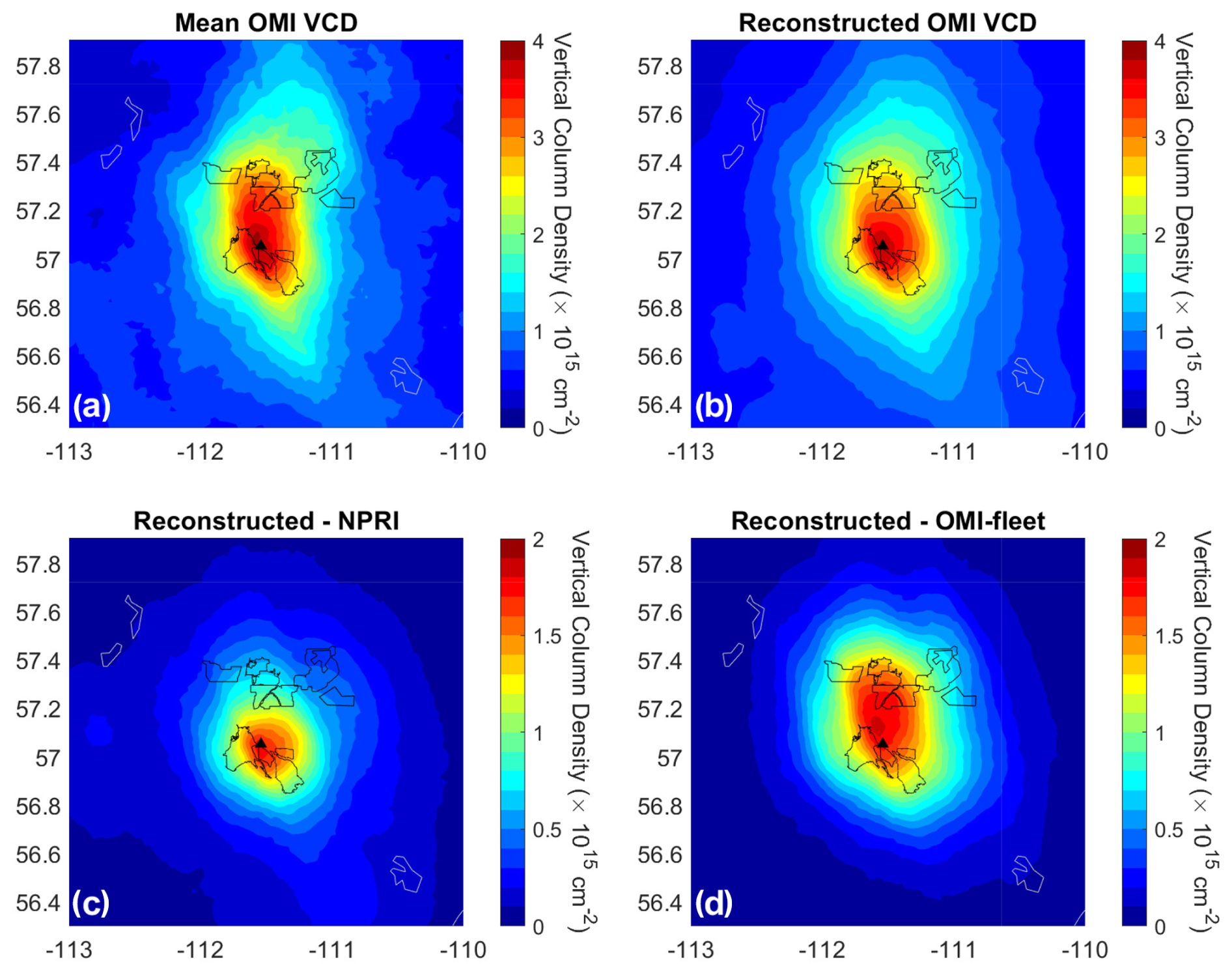
Figure 5 Summary of the multi-source emissions retrieval using 2005–2024 OMI NO₂ VCDs. (a) Mean OMI VCD over the surface mining region of the oil sands. The black lines denote the different mining operations (this panel is the same as Fig. 2a). (b) Reconstructed spatial distribution using the gridded emissions from Fig. 6b. Panels (c) and (d) are the VCDs reconstructed using emissions from the NPRI point source database and OMI-derived area fleet emissions, also from Fig. 6b. Note that the background is omitted from panels (b) and (c).

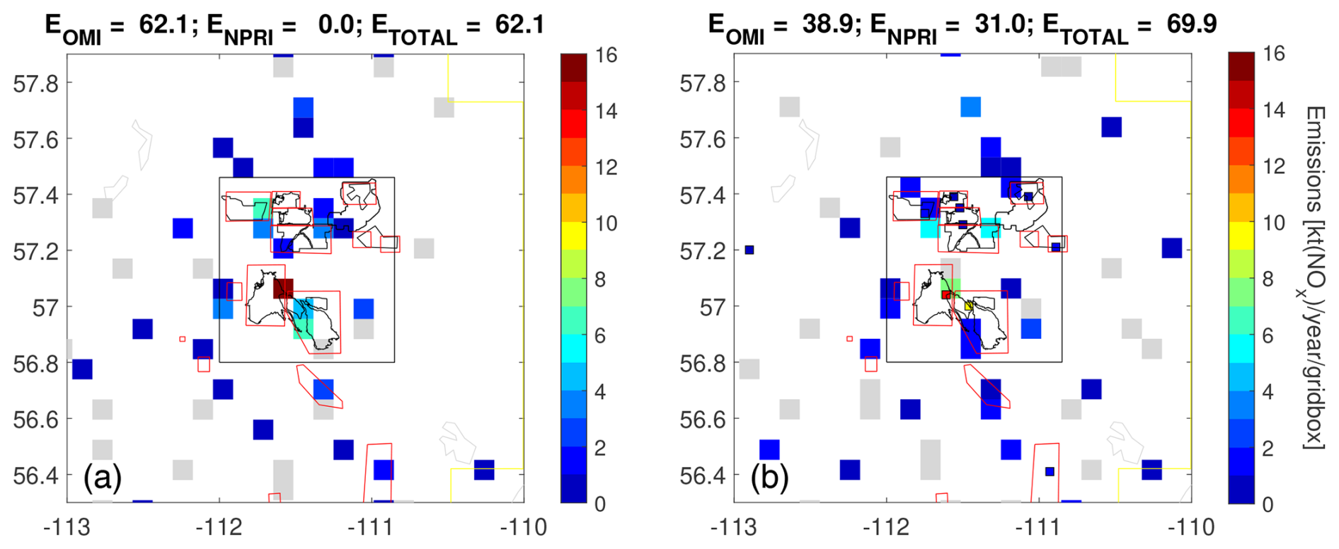
Figure 6 (a) OMI-derived NO_x emissions retrieved on an 8 × 8 km² grid using the multi-source method. These emissions represent the total of point and area sources. (b) As panel (a) but when point source emissions from the NPRI database, totalling 30.6 kt [NO₂] yr⁻¹, are specified. These gridded emissions represent area emissions only. Grey boxes represent retrieved emissions between 0 and 0.5 kt [NO₂] yr⁻¹. In panel (a) the total emissions within the box is 63.5 kt [NO₂] yr⁻¹; in panel (b) the total is 69.9 kt [NO₂] yr⁻¹, where 30.4 kt [NO₂] yr⁻¹ was specified and the remaining 39.5 kt [NO₂] yr⁻¹ was derived from the multi-source method.

Initially all OMI observations spanning 2005–2024 are analyzed together, and so a value of τ=3.2 h (see Fig. 2) is used. Performing the multi-linear fit provides a grid of retrieved NO_x emissions. A comparison of the mean VCD map with the reconstruction using these retrieved gridded emissions is given in Fig. 5a–b. The multi-source reconstruction now closely resembles the observations and is much more realistic than the point source reconstruction from Fig.  2d. The map of retrieved, gridded emissions used for Fig. 5b is shown in Fig. 6a. The emissions map shows large values over the surface mines, as expected, with the largest corresponding to the upgrader at the Syncrude Mildred Lake and Suncor facilities. Total surface mining emissions, calculated by summing grid boxes within the rectangle shown, are 62 kt [NO₂] yr⁻¹. Outside of this box, other small but non-zero emissions can be seen. Some of these correspond to known NO_x sources such as the city of Fort McMurray, in situ mining operations, and other small non-oil and gas related sources. Some of the small but non-zero emissions retrieved are likely the result of systematic biases in the VCDs.

This retrieval grid is 31 × 31, totalling 961 grid boxes. An important issue is the degree of independence of each box. One would not expect OMI, with its ∼ 21 km pixels, to be able to resolve emissions on an 8 × 8 km² grid. The multi-source method is based on EMG plume functions which serve as the basis functions in the multi-linear regression, and the extent to which they are correlated can be used to help determine the ability of OMI to spatially resolve emissions. At a distance of 8 km, neighbouring OMI NO₂ plume functions have a correlation of 0.92. Given uncertainties in the data and approximations of the method, this confirms that OMI is unable to disentangle them. A more reasonable correlation threshold is 0.5, below which individual sources can be resolved. This is explored further in Appendix F, where Fig. F2 shows how achieving this 0.5 threshold separation distance, z_min, varies with σ and, to a lesser extent, τ. For OMI NO₂, it was found that sources must be separated by about 22 km.

The concept of a minimum distance being required to distinguish between neighbouring emissions is very important for satellite emissions monitoring. An expression relating z_min directly to satellite resolution, σ_pixel, can be estimated by combining Figs. F1 and F2. The result is shown in Fig. 7. Estimates for several satellite data products are shown. While longer-lived species tend to require a slightly larger separation, the main driver is spatial resolution. This figure suggests TROPOMI and TEMPO (Zoogman et al., 2017) are able to resolve NO_x emissions sources that are ∼ 9 and 7 km apart, respectively. This approach does not account for real data characteristics, source strength (and relative strength of the two sources), and quantity of data used. One might also argue that a correlation coefficient threshold of 0.5 is too stringent, and that perhaps 0.7 might be more appropriate.

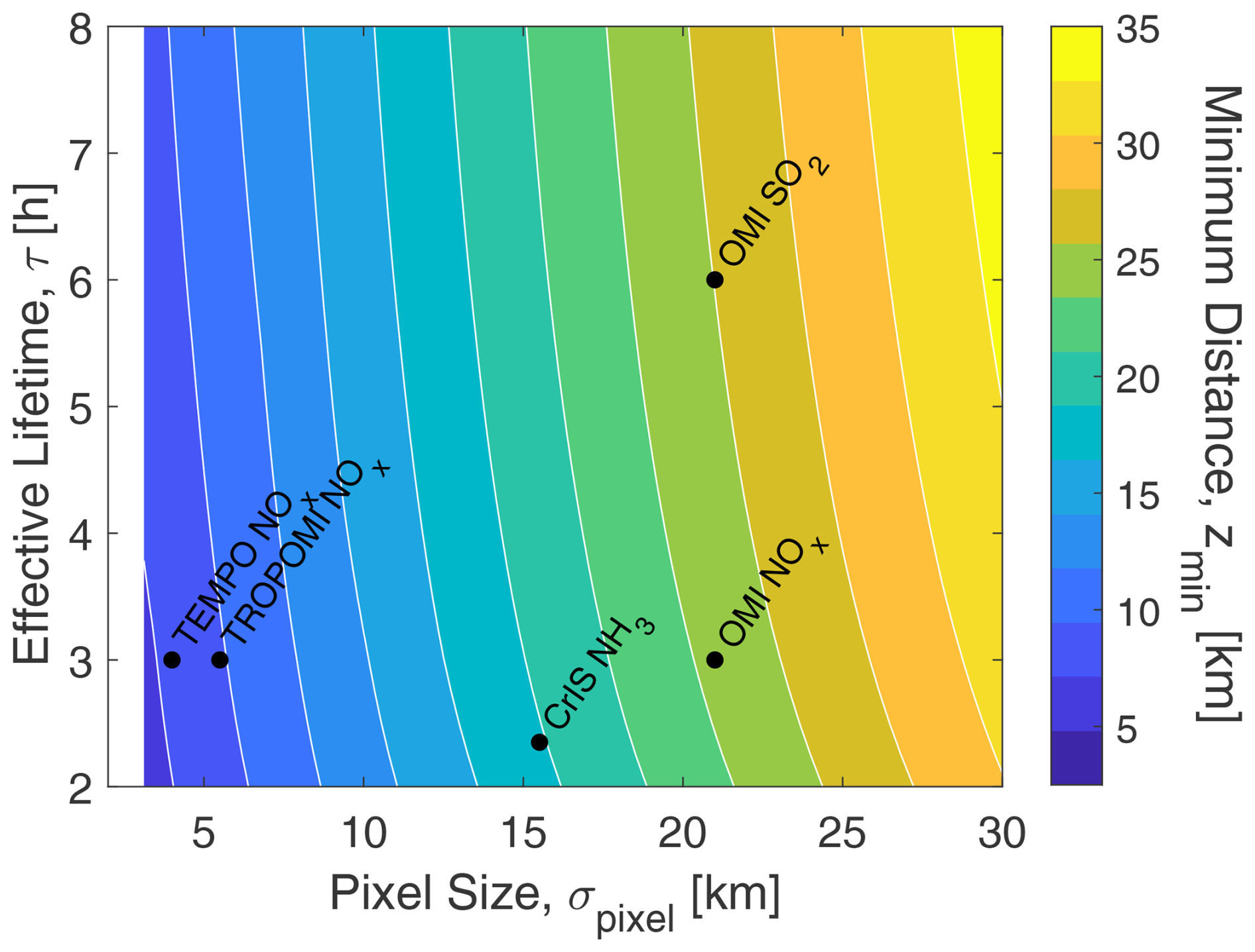
Figure 7 Minimum distance required to distinguish between two point sources as a function of satellite pixel resolution and effective lifetime. Values for several satellite emissions data products are also denoted.

The spatial scale of the individual surface mines is 5–20 km, but they are often separated by little or no distance. It is on this basis, albeit with one exception in Appendix D where this is explored further, OMI emissions derived from the multi-source method were simply summed over the surface mining box. It is noted that TROPOMI, with its superior spatial resolution, should be able to separate out emissions for the majority of these mines.

An alternative implementation of the multi-source method was used to derive vehicle fleet emissions. Recall that NO_x is primarily emitted by point sources, or stacks, and the off-road vehicle fleet. Some of the stack emissions make use of CEMS, and overall stack emissions are believed to be well known. Therefore, if the contribution to the OMI observations from the stacks can be removed, the remainder, from the fleet, can be fit using the same approach as above. This requires an initial step in which VCDs are reconstructed for each OMI observation, assuming stack emissions from NPRI, with these then subtracted from the actual OMI VCDs. This approach also allows an additional refinement as the height of the winds used for the prescribed stack emissions (400–800 m) can be different from those used to derive the off-road fleet emissions (0–400 m).

In practice this was done by first taking the NPRI emissions in the region, averaged over 2005–2023, and using these to reconstruct VCDs as shown in Fig. 5c. The peak over the southern mines reflects the larger emissions from the two upgraders separated by about 10 km. These VCDs were then subtracted from the OMI observations and the remainder used in the multi-source retrieval. The reconstructed total VCDs, those from the multi-source added to the NPRI VCDs from Fig. 5c, are virtually identical to those from Fig. 5b, and so they are not shown. Figure 5d shows the VCD reconstructed considering only the retrieved emissions which are attributed to the mine fleet. This VCD distribution is more homogeneous through the area, reflecting the more diffuse nature of this source.

The corresponding emissions map is shown in Fig. 6b, where the small squares represent the prescribed NPRI point source emissions, and the grid box values are the retrieved (fleet) emissions. Total (point + fleet) emissions for the two methods differ due primarily to how the wind height is handled. Had the same winds been used in both, then the totals would be the same (to within 0.1–0.2 kt [NO₂] yr⁻¹) and one could have obtained the same result by simply subtracting the NPRI total from that in Fig. 5a.

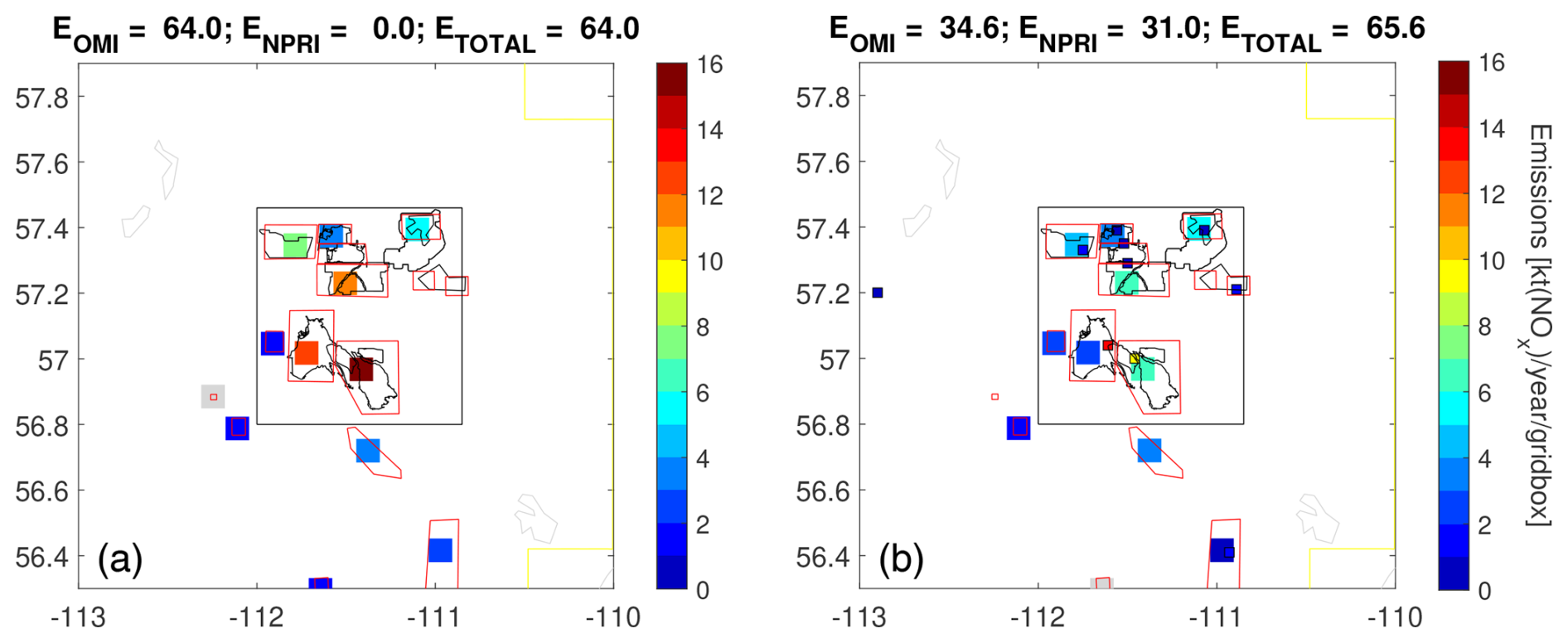
Figure 8 (a) OMI-derived NO_x emissions retrieved using the multi-source method where emissions locations are assigned to the centre of mining facilities. These emissions represent the total of point and area sources. (b) As panel (a) but when point source emissions from the NPRI database, totalling 30.6 kt [NO₂] yr⁻¹, are specified. In panel (a) the total emissions within the box is 65.6 kt [NO₂] yr⁻¹; in panel (b) the total is 66.3 kt [NO₂] yr⁻¹, where 30.4 kt [NO₂] yr⁻¹ were specified and the remaining 35.9 kt [NO₂] yr⁻¹ were derived from the multi-source method.

Two more variants of this method are considered. Here, instead of a grid, potential source locations are limited to known emissions sites, including industry and the city of Fort McMurray. The resultant emissions maps are shown in Fig. 8. The squares reflect the emissions retrieved from each location. No attempt was made to account for the spatial scale of the mining operation; rather each was treated as a point source. As can be seen, the emissions maps are similar overall to the grid approach in both spatial distribution and surface mining total.

3.3 Emissions time series

As with the point source method, emissions using the multi-source approach were also derived considering 3-year time increments and using the effective lifetime time series from Fig. 3b. Maps of average VCD maps and their reconstructions are shown in Figs. D2 and D3, respectively. The emissions time series is shown in Fig. 9.

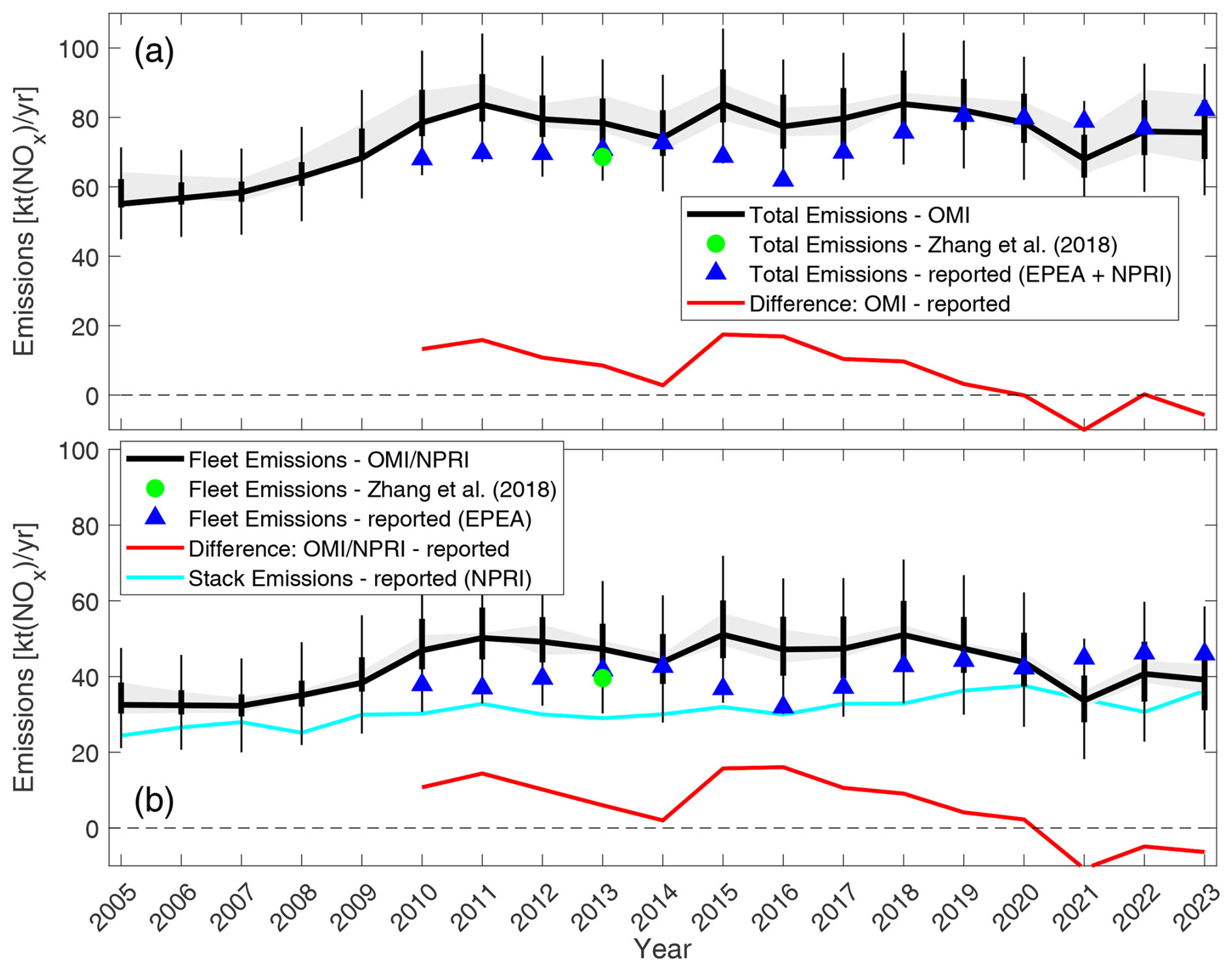
Figure 9 Comparison of reported and OMI-derived NO_x emissions for (a) total and (b) fleet in the oil sands surface mining region. Thick error bars represent the random uncertainty, and thin error bars represent total (random and systematic) uncertainty. The shading indicates the variability among the various methods for deriving emissions (and is included in the total uncertainty).

Several variations of the multi-source were utilized, analogous to what was discussed in Sect. 3.2. A summary of these is given in Table E1. Considering these together with the point source results shows relatively little variation amongst them, typically a few percent with the largest being 15 % for a single 3-year period. Based on this and the difficulty in determining which method is “best” it was decided to take the mean of several methods, according to Table E1), as the final emissions value, with their variability taken as a measure of uncertainty.

Emissions are found to steadily increase over the OMI record from about 55 to 80 kt [NO₂] yr⁻¹, as seen in Fig. 9a, between 2005 and 2010, remaining roughly flat thereafter. Comparing total NO_x emissions, there is good overall agreement between OMI and the bottom-up estimates. The bottom-up values are consistently 0–15 kt [NO₂] yr⁻¹ smaller but within the OMI uncertainties. As the time period over which the NO_x emissions were found to increase (2007–2011) generally corresponds to the main expansion of the OMI row anomaly, emissions over the entire time series were recalculated but restricted only to track positions that were unaffected by the anomaly over the entirety of the mission to date. Considering the previous criteria of excluding pixels near the edge of the detector due to their coarse spatial resolution, only track positions between 8 and 23 were considered for this sensitivity study. Emissions calculated in this way were found to be minimally impacted, reaching roughly 3 kt [NO₂] yr⁻¹ in 2007, well below the calculated precision, and not changing the overall time series picture.

Fleet emissions, as derived by prescribing stack emissions, are shown in Fig. 9b. These generally follow the total emissions since the stack emissions only display a modest increase with time. The magnitude of the fleet emissions uncertainties is taken to be the same as that from the total emissions in Fig. 9a. Fleet emissions were found to comprise about 60 % of the total emissions. Neither reported nor satellite emissions show much variation over the 2010–2023 period for which both are available.

4 Discussion

As can be seen in Fig. 10a, the average rate of increase in fleet emissions is 1.3 % yr⁻¹ from 2005, with the bulk of the increase occurring 2005–2011. Yet the rate of increase in the mass of oil sands mined, which is generally considered a reasonable proxy for fleet emissions since they must transport the bitumen from the mine to the separation facility, is considerably larger. This apparent discrepancy may be reconciled by considering the evolving standards as the Canadian vehicle NO_x emissions transitioned from unregulated (Tier 0) to present-day standards (Tier 4i/4) (Environment Protection Agency, 2016). As part of an agreement with the United States, Canada adopted the EPA Tier 1 standard for heavy-duty, non-road vehicles (9.2 g [NO_x] kWh⁻¹) in 2000, the Tier 2 standard (6.4 g [NO_x] kWh⁻¹) in 2006, and then the Tier 4 standard (3.5 g [NO_x] kWh⁻¹) in 2012. There were no Tier 3 standards for this class of vehicle. Lower-tier trucks could still be used as these stricter regulations were phased in, but any new or replacement engines were required to comply with the standard of the time. With a typical engine lifetime of 12 years, the benefits of Tier 4 regulations will not be fully realized until the late-2020s (M. J. Bradley & Associates, 2008).

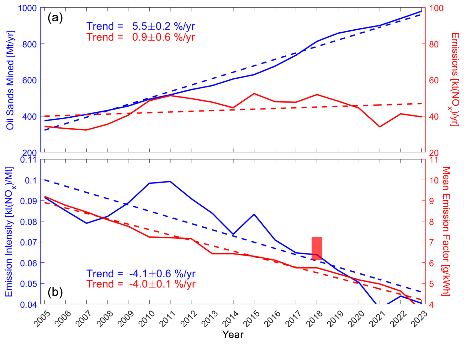
Figure 10 (a) Time series of mass of oil sands mined and fleet emissions from OMI. Dashed lines are linear trend lines, with the calculated trends indicated. (b) Emission intensity (defined as the ratio of fleet emissions to oil sands mined) and an estimated mean emission factor (see text). The shaded red bar show an estimate of the mean emission factor using reported fleet data.

An emission intensity metric is defined here as the mass of NO_x emitted from the mining fleet per unit mass of mined oil sands, and this is shown in Fig. 10b. It is seen to decrease at 3.8 % yr⁻¹. To contrast this with an expected decline, the composition of the vehicle fleet is required. Unfortunately, it was only in 2018 as part of the new Alberta Emissions Inventory Reporting (AEIR) program that industry was required to report on fleet composition. While useful as a snapshot, this means there is no direct information on fleet evolution over the study period.

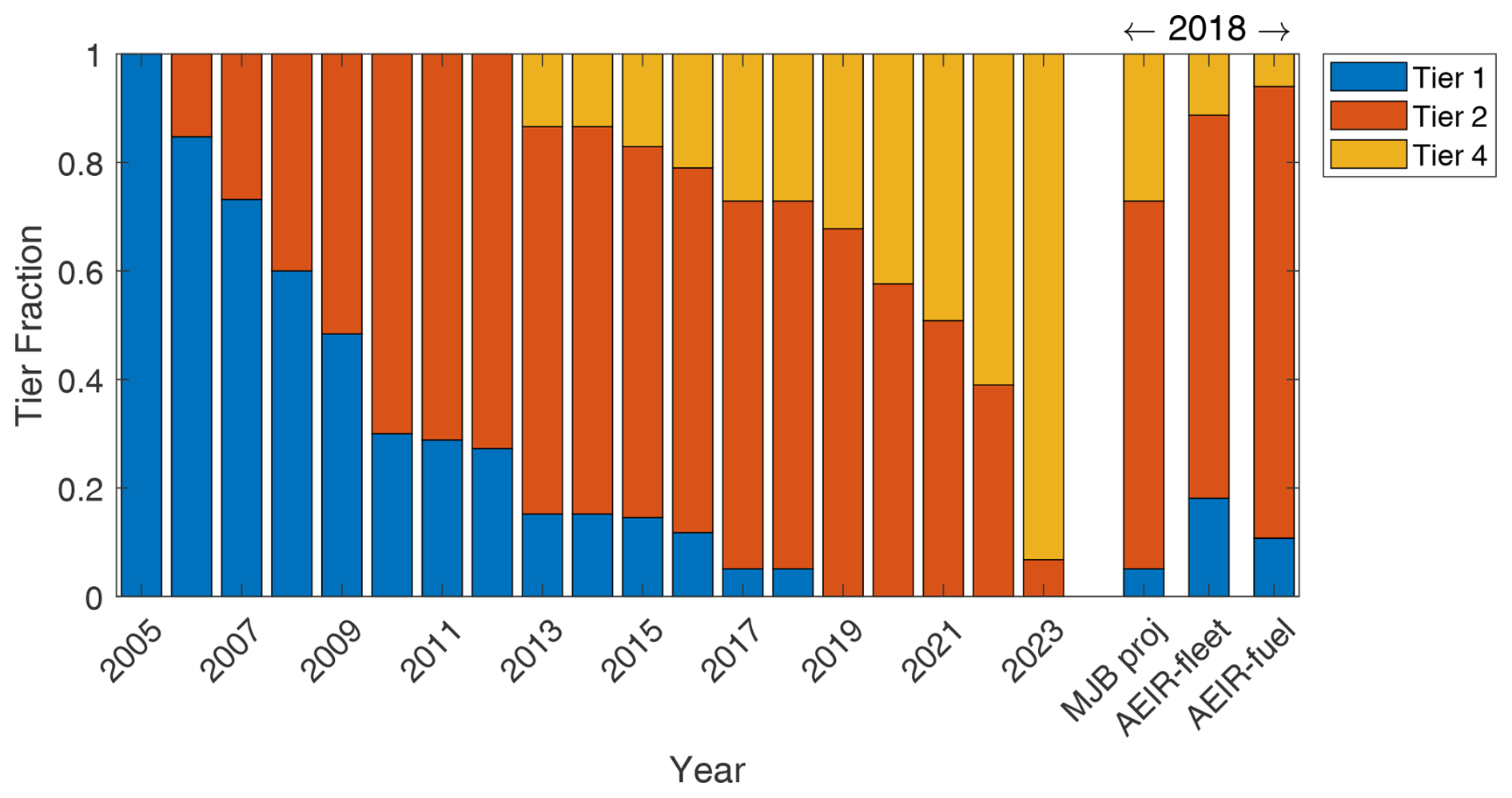
Figure 11 Composition of mine fleet according to emissions tier, shown as a cumulative fraction. The time series shows projections from the M. J. Bradley & Associates (2008) study for large (> 750 hp), diesel vehicles. The three on the right compare 2018-projected values with the 2018 AEIR fleet report, total vehicles, and fuel consumed.

One alternative is a study delivered to Environment and Climate Change Canada in 2006 projecting the make-up of the mine fleet going forward (M. J. Bradley & Associates, 2008). Their projected mine fleet composition is shown in Fig. 11. This study predicted the largest growth between 2005 and 2010, where total vehicles increased from about 200 to 500, before levelling off at 600. This is the reason for the rapid increase in Tier 2 fraction. For comparison the AEIR data indicate a fleet size of 730 large (> 750 hp) trucks in 2018. A comparison with AEIR reported tier fractions is also shown in Fig. 11, where the weighting was done using total vehicles as a function of tier as well as fuel consumed by tier. There is general agreement with the projections, with Tier 2 vehicles composing the majority. One difference is the fraction of Tier 1 vs. Tier 4, with there being fewer Tier 4 vehicles than projected. Note that one large facility in the AEIR did not report which tier their vehicles belonged to, and so these trucks were excluded from this analysis.

As a second alternative, a simple model was constructed beginning with 205 Tier 1 trucks in 2005. Trucks were increased at the same rate as total bitumen mined, with a fraction of existing trucks being replaced each year with ones at the current tier. Assuming a 12-year lifetime (M. J. Bradley & Associates, 2008), where for simplicity lifetime is taken as an e-fold such that 8.0 % of trucks (or engines) were replaced each year. As suggested by the bitumen-mined time series in Fig. 10a, the total trucks increased steadily and doubled over the time frame considered. The largest difference between this approach and the M. J. Bradley & Associates (2008) and AEIR data is the difference in Tier 2 truck fraction.

While the 730 large (> 750 hP) diesel trucks from the 2018 AEIR mine fleet report make up fewer than half of the 1610 total vehicles listed in the report, they accounted for 92 % of the fuel consumed and so would also be responsible for the large majority of NO_x emissions. Overall, the AEIR total number of trucks and the breakdown among the tiers agree better with the projections. Nonetheless, the model remains a useful sensitivity study.

Assuming each truck uses the same amount of fuel and emits according to its standard, the weighted average emission factor can be computed for the projected fleet compositions. This was done by weighting the Tier 1, 2, and 4 emission standard (9.2, 6.4, and 3.5 g [NO_x] kWh⁻¹) with the fractions from Fig. 11. Thus 2005 would have a value of 9.2 since it is entirely Tier 1, and 2006 would be slightly smaller since it is about 85 % Tier 1 and 15 % Tier 2. This metric, from Fig. 10b, changes at −4 % yr⁻¹, a decrease that is essentially the same as that for the emissions intensity. In 2018, the emission intensity as defined above had declined by about 31 % since 2005, and the mean emission factor using the fleeted projections had declined by 46 %. These can be compared with the change in AEIR mean emission factor, assuming an initial value of 9.2 g kWh⁻¹, the Tier 1 NO_x standard. A decline of 21 %–31 % is calculated, with the range depending on whether total vehicles or total fuel consumed was used to weight the mean.

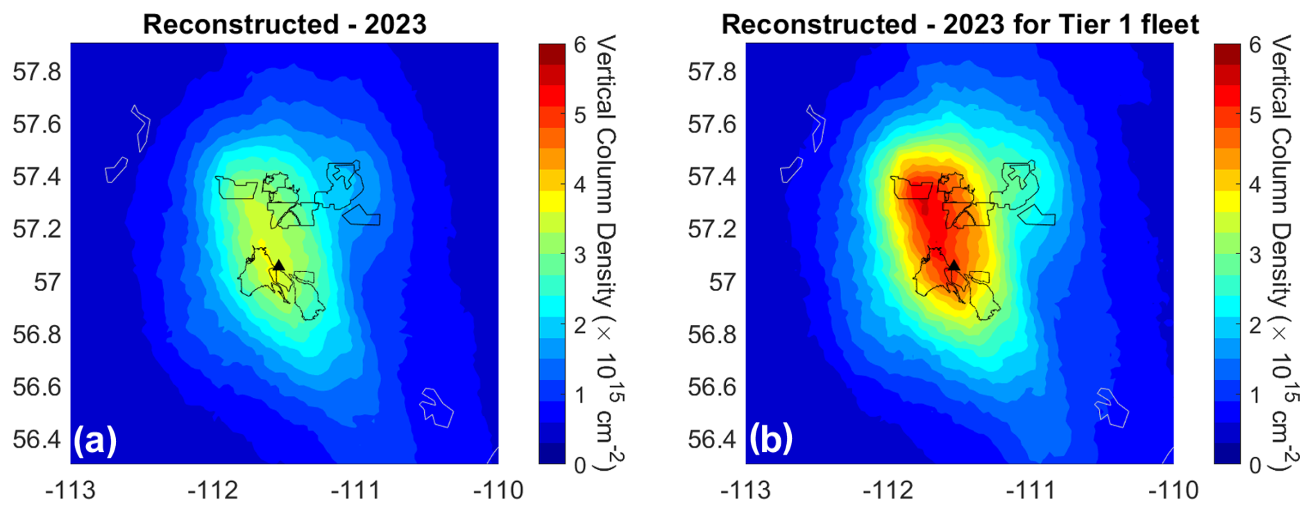
Figure 12 (a) Reconstructed 2023 NO₂ VCD map using OMI-derived fleet emissions and NPRI point source emissions. (b) As panel (a) but with fleet emissions doubled to approximate expected VCD distribution assuming Tier 1 emission standards. Note the colour bar range here is different as compared with previous figures.

Figure 10b suggests that the efficacy of the EPA emissions standards, at least in the case of the oil sands fleet, adopted by Canada is at or close to the level expected. Considering Fig. 10b further, emission intensities remained constant at 2005 levels, with 2005 being the final year of Tier 1 standards, and increased with oil sands mined (5.6 % yr⁻¹) instead of that observed (1.3 % yr⁻¹). The fleet emissions reduction brought about from the adoption of Tier 2 and later Tier 4 standards, relative to Tier 1, is roughly 40 kt [NO₂] yr⁻¹ in 2023. To put this into context, a value of 40 kt [NO₂] yr⁻¹ is comparable to that emitted from an urban area (minus local industry) of 5 million people using an approximate value for a per-capita rate of emissions of 7 kt [NO₂] yr⁻¹ per 1 million people (Fioletov et al., 2022) or not quite half the roughly 100 kt [NO₂] yr⁻¹ emitted from the greater Toronto area (Goldberg et al., 2019b) in the summer. Over the past 19 years, this amounts to roughly 400 kt [NO₂] less NO_x being emitted as a result.

The multi-source method can also be used to examine emission scenarios. For example, the impact on the average NO₂ VCD distribution due to a 20 % reduction in fleet emissions or the opening of a new operation emitting 15 kt [NO₂] yr⁻¹ could readily be evaluated. This is demonstrated in Fig. 12 by comparing NO₂ VCD maps calculated using 2022–2024 OMI-derived fleet and NPRI emissions to VCDs derived using these fleet emissions increased by 50 % as might be expected for Tier 1 vehicles. In order words, Fig. 12b represents the scenario avoided by implementing Tier 2 and later Tier 4 standards.

5 Summary and conclusions

OMI observations of NO₂ tropospheric VCD were used to quantify NO_x emissions from the surface mining region of the Canadian oil sands between 2005 and 2024. Two different, though related, emissions algorithms were found to give very similar results. One assumes all emissions emanate from a single (near) point source, whereas the other treats the area as multiple point sources or an area source. These methods utilize both wind speed and direction from a meteorological reanalysis and a two-dimensional exponentially modified Gaussian (EMG) plume model.

OMI-derived emissions were found to increase from 55 to 80 kt [NO₂] yr⁻¹ between 2005–2011 and then remain roughly flat afterwards. These were found to be within 15 % of reported emissions, but given a 20 % uncertainty in the OMI emissions, this difference is not significant. In an additional variation of this methodology, OMI observations were combined with reported point source emissions to derive the more uncertain emissions component from the large off-road (heavy-hauler) mining fleet. These were found to make up about 60 % of total NO_x emissions, consistent with about 55 % from reported emissions. The 0.9 % yr⁻¹ increase from this source and the 5.5 % yr⁻¹ increase in bitumen mined, generally a good proxy for fleet emissions, can be reconciled by considering the evolution of the mine fleet over this period. OMI is therefore able to track the transition from US EPA Tier 2 standards (in 2006) through to Tier 4 (in 2012) to the present and in doing so demonstrate the efficacy of this policy. Furthermore, this analysis shows that had the fleet remained at Tier 1 (emission intensity), the surface mines would currently be emitting an additional 40 kt [NO₂] yr⁻¹, or an additional 35 % of the current total, an amount equivalent to that from a city of ∼ 5 million inhabitants (Fioletov et al., 2022).

Some improvements over other studies include more consistent, emissions-based scaling to convert NO₂ to NO_x, which was found to give a conversion factor about 10 % larger than a simple NO_x $/$ NO₂ concentration ratio. Another improvement lay in the use of an evolving effective lifetime, reflecting the fact that NO₂ impacts its own loss rate. In addition to emissions, this work better connects the point source and area source emissions methods and discusses the interpretation of fitting parameters and the ability to resolve emissions from sources in close proximity.

Appendix A: The oil sands surface mining facilities

The individual mining facilities are shown in Fig. A1.

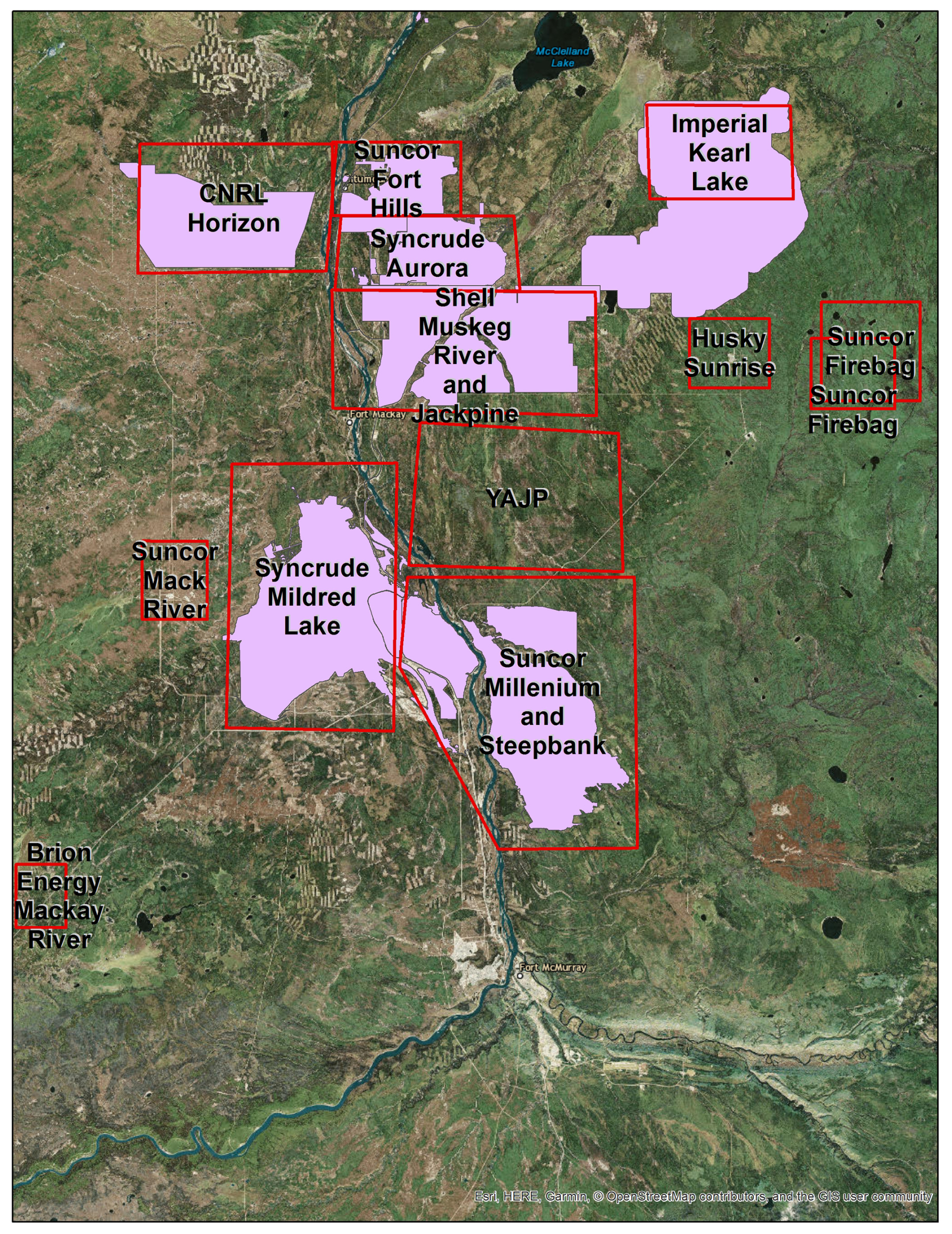
Figure A1 Location and name of all mining facilities.

Appendix B: The two-dimensional exponentially modified Gaussian plume function

The two-dimensional exponentially modified Gaussian (EMG) is used to model the vertical column density, VCD, distribution of the plume as seen from a satellite instrument. It is preferred over the traditional Gaussian plume (Stockie, 2011) as it better accounts for the finite spatial extent of the source itself and the relatively coarse spatial resolution of the satellite observations being utilized. Mathematically it is the convolution of a two dimensional Gaussian (i.e. integrated through the vertical dimensional) and an exponential. It depends on the cross-wind distance, x, and the downwind distance, y, each in kilometres and relative to the location of the emission source, and the wind speed, s, in km h⁻¹ and where the wind is aligned in the y direction. Carrying out the convolution leads to the following functional form, described by Eqs. (B1)–(B5),

$$\begin{array}{}\text{(B1)}& \mathrm{VCD}(x,y,s)=\mathrm{EMG}(x,y,s)=a\cdot f(x,y)\cdot g(y,s),\end{array}$$

where the functions f and g are

$$\begin{array}{}\text{(B2)}& {\displaystyle }f(x,y)={\displaystyle \frac{\mathrm{1}}{{\mathit{\sigma }}_{\mathrm{1}}\sqrt{\mathrm{2}\mathit{\pi }}}}\cdot \exp \left(-{\displaystyle \frac{x^{\mathrm{2}}}{\mathrm{2}{\mathit{\sigma }}_{\mathrm{1}}^{\mathrm{2}}}}\right)\text{(B3)}& {\displaystyle }\begin{array}{rl}g(y,s)=& {\displaystyle \frac{{\mathit{\lambda }}_{\mathrm{1}}}{\mathrm{2}}}\cdot \exp \left({\displaystyle \frac{{\mathit{\lambda }}_{\mathrm{1}}({\mathit{\lambda }}_{\mathrm{1}}{\mathit{\sigma }}^{\mathrm{2}}-\mathrm{2}y)}{\mathrm{2}}}\right)\\ & \cdot \mathrm{erfc}\left({\displaystyle \frac{{\mathit{\lambda }}_{\mathrm{1}}{\mathit{\sigma }}^{\mathrm{2}}-y}{\sqrt{\mathrm{2}}\mathit{\sigma }}}\right)\end{array}\end{array}$$

and where

$$\begin{array}{}\text{(B4)}& {\displaystyle }{\mathit{\sigma }}_{\mathrm{1}}=\left\{\begin{array}{ll}\sqrt{{\mathit{\sigma }}^{\mathrm{2}}+\mathrm{1.5}y},& y>\mathrm{0}\\ \mathit{\sigma },& y\le \mathrm{0}\end{array}\right.\text{(B5)}& {\displaystyle }{\mathit{\lambda }}_{\mathrm{1}}={\displaystyle \frac{\mathrm{1}}{\mathit{\tau }\cdot s}}.\end{array}$$

The a factor represents the concentration enhancement by the source and is directly proportional to the mass of the enhancement, m; σ is the parameter describing the width of the Gaussian (in km); τ is the effective lifetime (in hours); and $\mathrm{erfc}\left(x\right)=\frac{\mathrm{2}}{\sqrt{\mathit{\pi }}}{\int }_x^{\mathrm{\infty }}{e}^{-t^{\mathrm{2}}}\mathrm{d}t$. This formulation is the same as in Fioletov et al. (2015) except that y has been replaced by −y so that distances downwind of the source are now positive. The emission rate is given by $E=m/\mathit{\tau }$, and ultimately the distribution is characterized by (E, τ, σ). See Fioletov et al. (2015) for additional information.

Equation (B2) can be recognized as the standard Gaussian describing the cross-wind distribution and is a function of the downwind distance via the diffusion term embedded in σ₁. In Eq. (B3), g(y,s) is a convolution of a Gaussian and exponential in the downwind direction, where the exponential accounts for first-order loss due to chemistry and deposition (with decay rate τ and thus the decay being $\sim \exp [-y/(\mathit{\tau }\cdot s\left)\right]$, and ${\mathit{\lambda }}_{\mathrm{1}}=\mathit{\lambda }/s$ from Eq. B5). Figure B1 shows a sample plume.

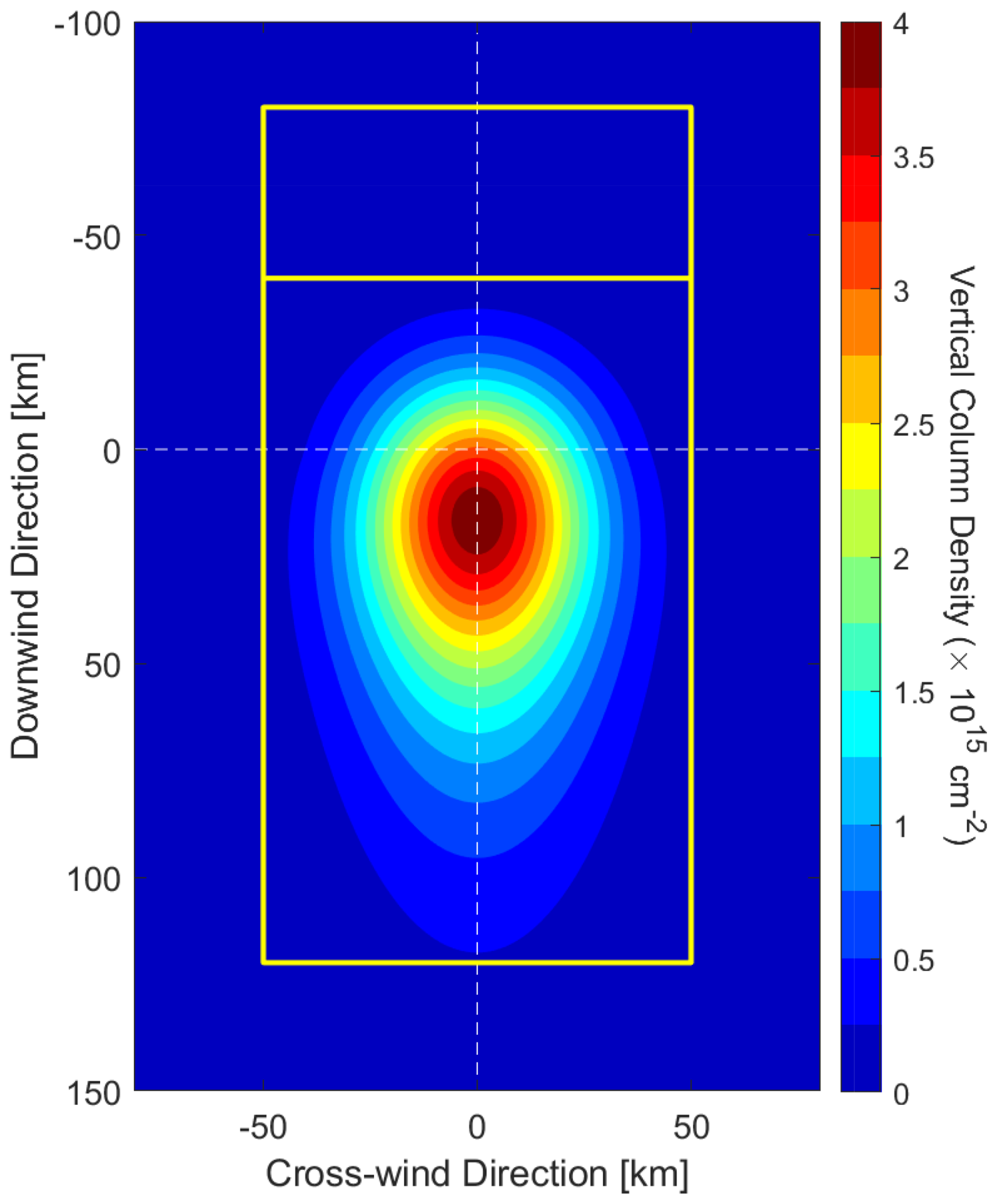
Figure B1 Sample of NO₂ VCDs generated using the EMG plume function as defined in Eqs. (B1)–(B5). In this example E=50 kt [NO₂] yr⁻¹, τ=2.8 h, and σ=18 km, and a constant wind speed of 12 km h⁻¹ was specified. The upper box shows the domain used to calculate the background, and the lower box shows the domain over with the EMG function is fit. The limits in x are ±50 km and $y=-\mathrm{80}$ to −40 km for the background and $y=-\mathrm{40}$ to 120 km for the fit. No background NO₂ was added in this example.

Appendix C: Implementation of the point source method

The point source method involves a non-linear fit of OMI VCDs to the EMG as detailed in Appendix B. Here, the solution is obtained using the non-linear least-squares solver “lsqnonlin.m” in MATLAB. The non-linear terms are the lifetime and width parameters, whereas the mass is a linear scaling of the EMG.

It is important to note that the reference location must be specified as part of the point source method, where the reference location is the location of the emission source. In the case of a somewhat extended, or pseudo-point source, the centre of the emission source(s) is used. Here, wind information comes from the ECMWF ERA-Interim or ERA-5 reanalyses (Dee et al., 2011) interpolated in space and time to the location of each OMI pixel.

In order to combine many overpasses where wind direction is constantly changing, a wind rotation scheme is used (Pommier et al., 2013) where the location of the OMI pixel (as denoted by the pixel centre) is rotated about the reference location so that wind directions are aligned (see also Fioletov et al., 2015).

Background levels of NO₂ must be accounted for when deriving NO_x emissions, where background in this context refers to the NO₂ that would be present if the source in question were removed. This can be done by additionally including a constant as part of the EMG fit, or, as here, an upwind average can be determined and subtracted from all VCDs before the fit. This is illustrated in Fig. B1, which shows a sample EMG plume and the two domains used for the fit. The average over the upwind box (between $x=\pm \mathrm{50}$ and $y=-\mathrm{80}$ to −40 km) is used to calculate the background, which accounts for any NO₂ not emitted locally, as well as potential offsets due to an imperfect stratospheric removal. The larger box is the domain over which the non-linear fit is performed ($x=\pm \mathrm{40}$ km and $y=-\mathrm{40}$ to 120 km).

While the fitting is carried out in the rotated frame, the agreement with the original mean OMI VCD distribution can be assessed by taking the fitted EMG and rotating it back to the original co-ordinates. This is called the reconstruction, and it highlights one advantage of using this 2D approach where spatial information is not lost in an averaging.

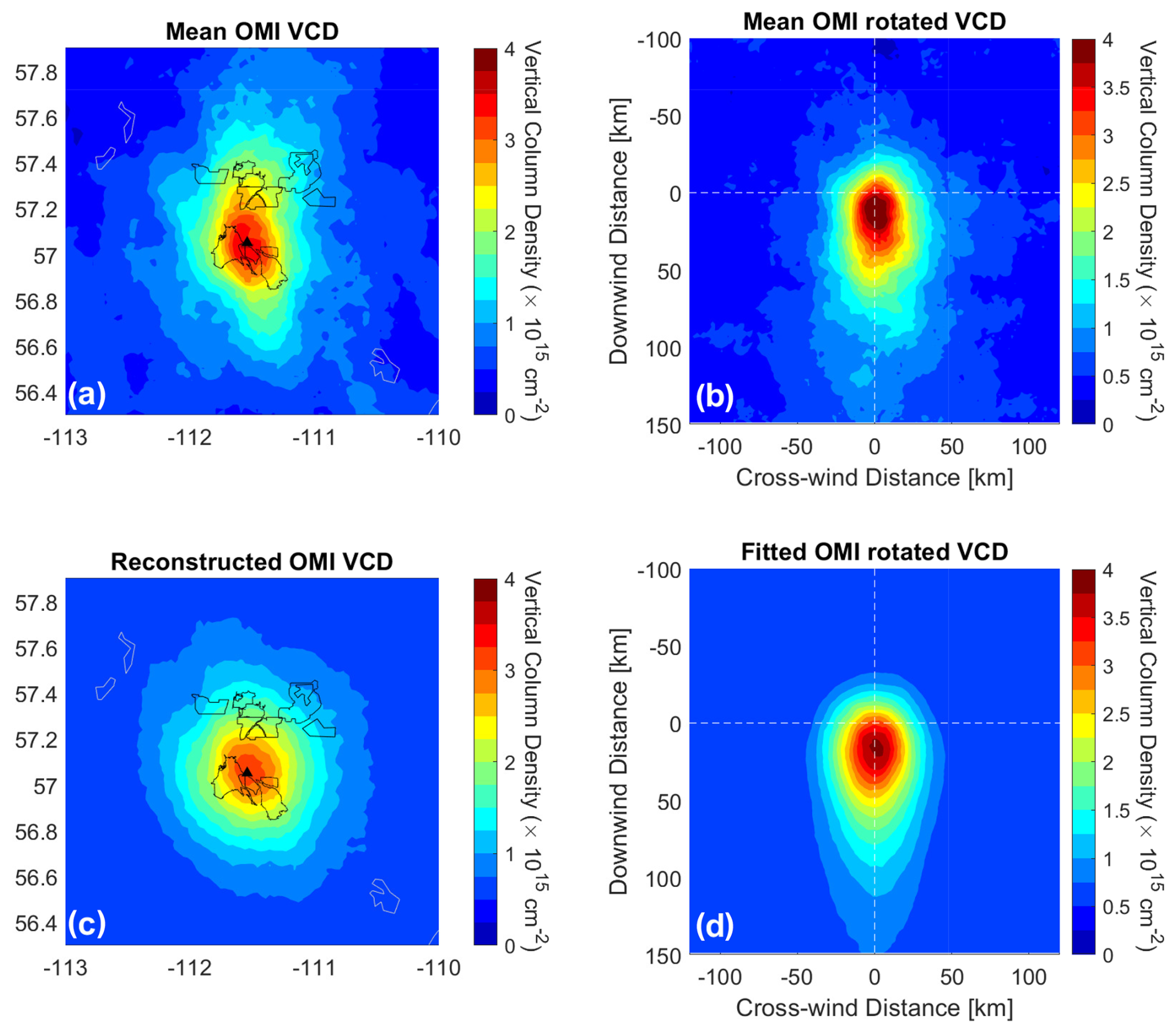
Figure C1 Summary of the point source emissions procedure using 2005–2007 OMI NO₂ VCDs. (a) Mean OMI VCD over the surface mining region of the oil sands. The black lines denote the different mining operations; (b) mean OMI VCD after rotation showing plume-like structure; (c) reconstructed spatial distribution using EMG plume and fitted parameters; and (d) fit to rotated VCD using 2D EMG plume function, with fitted parameters of E=55.3 kt [NO₂] yr⁻¹, τ=2.8 h, and σ=17.6 km. The black triangles in panels (a) and (c) show the reference location used in the emissions retrieval that corresponds to the (0,0) point in panels (b) and (d).

Figure 2 shows the mean OMI VCD, OMI-rotated VCD, fitted VCD, and reconstructed VCD plots considering all years of OMI data. Analogous plots are shown here but considering only a single 3-year period, 2005–2007, in Fig. C1. Each 3-year period considered, even in later years with reduced data, is comparable in fit quality. This time period was chosen as it predates much of the expansion of the northern mines and thus better represents a point source as reflected by a smaller width parameter, σ=17.5 km vs. 20.6 km, and smaller total emissions, E=55 vs. 70 kt [NO₂] yr⁻¹, as compared to the all-year analysis.

Appendix D: Implementation of the multi-source method

To determine emissions from multiple sources, a related method has been developed (Fioletov et al., 2017; McLinden et al., 2020) whereby each (potential) source location is treated as an EMG plume. The total VCD is therefore the sum over all plumes, plus the background term(s),

$$\begin{array}{}\text{(D1)}& \mathrm{VCD}(x,y,s)=a_{\mathrm{0}}+\sum _{i=\mathrm{1}}^N{a}_i\cdot \mathcal{R}\left[\mathrm{EMG}(x,y,s)\right],\end{array}$$

where N is the total number of sources, and x, y, and s are as in Appendix A and are specific to each type of emissions. The downwind and cross-wind distances, y and x, will differ from location to location as these are distances, after rotation, between all pixels being considered and source i. Furthermore, there will be some modest variation in wind speed, s, as these are also location-specific and derived from an interpolation of the ERA-5 (31 km; Hersbach et al., 2020) wind fields. The EMG function is also as above, but here the ℛ denotes that EMG was transformed, or rotated, back into the original latitude and longitude co-ordinates. These rotated EMG functions then serve as basis functions in a system of linear equations in latitude–longitude space. The non-linear coefficients in the EMG Gaussian terms, f and g (Eqs. B2 and B3), are specified and not fit. The MATLAB function lsqlin.m was used with a positive constraint placed on all values of the fitted a_i coefficients, which are linearly related to the emission rate. Here a constant, a₀, is also fitted and represents the background NO₂ that would be present in absence of these local sources. The constant can be replaced by a more complicated background term as has been done in other studies, such as a plane or a series of polynomials (Fioletov et al., 2022; Wren et al., 2023). However, here a constant was found to be sufficient since only a relatively small domain is being considered. In this work source, locations were specified as being either on a grid or at the centre of each known source.

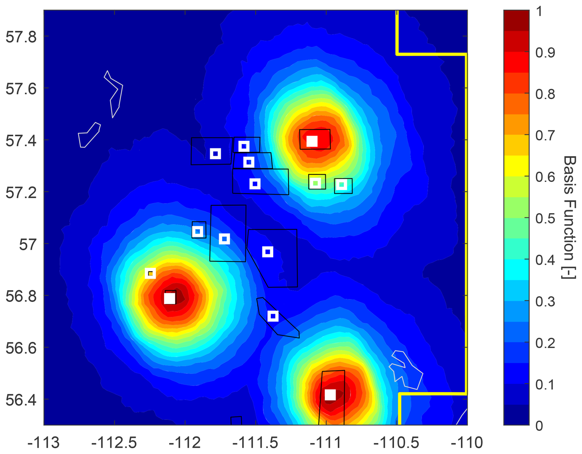
Figure D1 Examples of averaged OMI NO₂ multi-source fit basis functions. The black polygons outline the boundaries of the NO_x source, and the white squares are the locations where the emissions are allowed to emanate. For three locations, indicated by the filled squares, the average plume shape is shown. An averaging radius of 12 km was used.

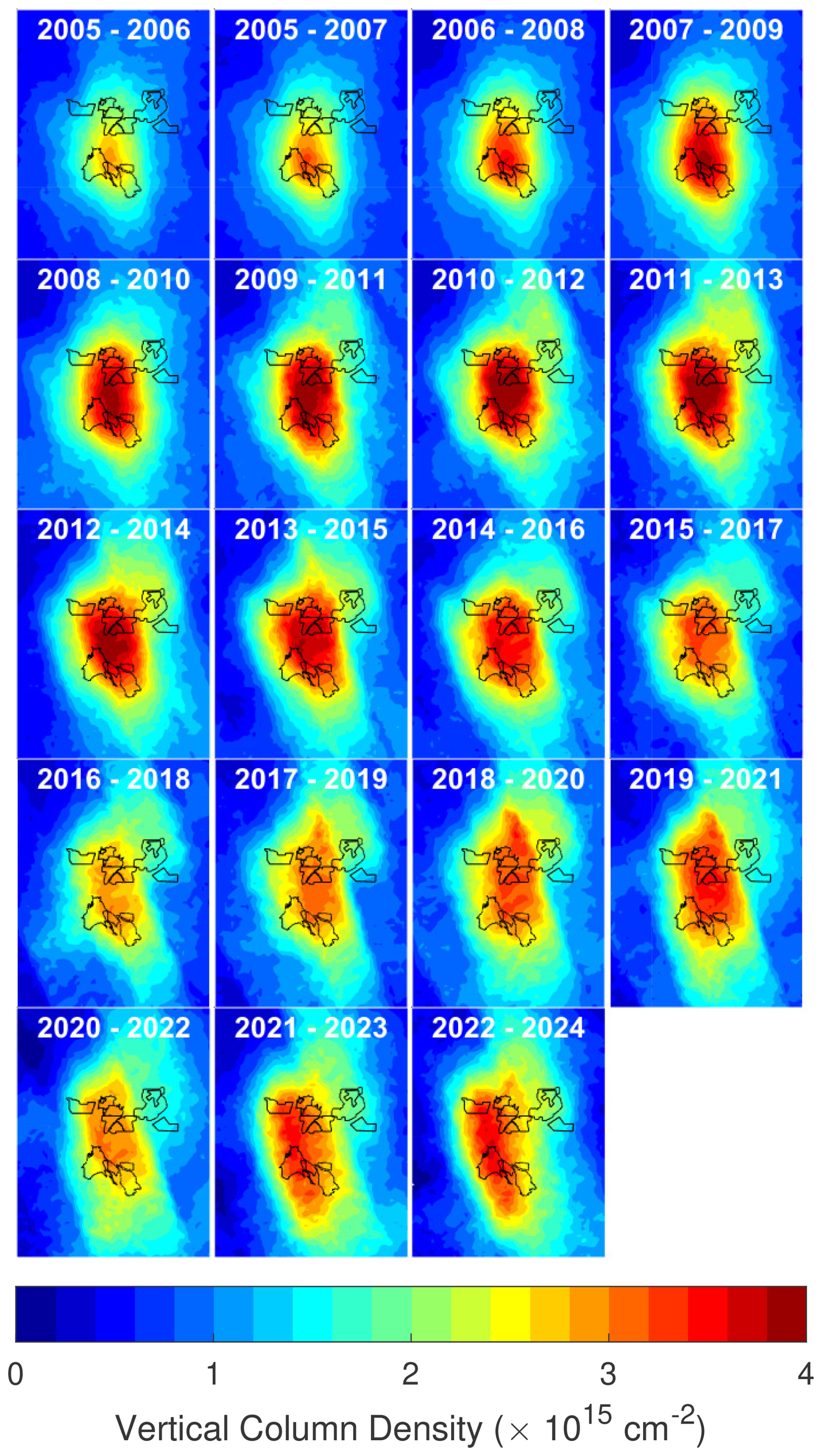
Figure D2 Three-year mean OMI NO₂ vertical column density (VCD) distributions over the surface mining. An averaging radius of 12 km was used.

The idea behind the multi-source method is better illustrated using Fig. D1. In this example, emissions are allowed to emanate (although the magnitude of the emissions may be zero) from 14 locations identified by the white squares, each of which corresponds to a known source of NO_x, either a surface mine, in situ mine, or community, in the domain under consideration. For locations indicated by the filled squares, the average rotated EMG plume is shown. Here, only three of the potential emissions locations are shown for clarity, but in the fitting procedure, each square (open or filled) would have a similar-looking distribution. The distribution associated with each location represents the average NO₂ VCD spatial pattern expected and is the basis function in the multi-linear fit. The slight elongation of the pattern reflects the fact that W and SW winds are the preferred wind direction. By fitting the OMI VCDs to Eq. (D1), a coefficient or scaling for each of these is determined that represents the emissions from that location. The sum over all sources, also called the reconstruction, should be in good agreement with the OMI distribution. Figure D3 can be compared with Fig. D2 to confirm the general consistency for all 3-year periods analyzed.

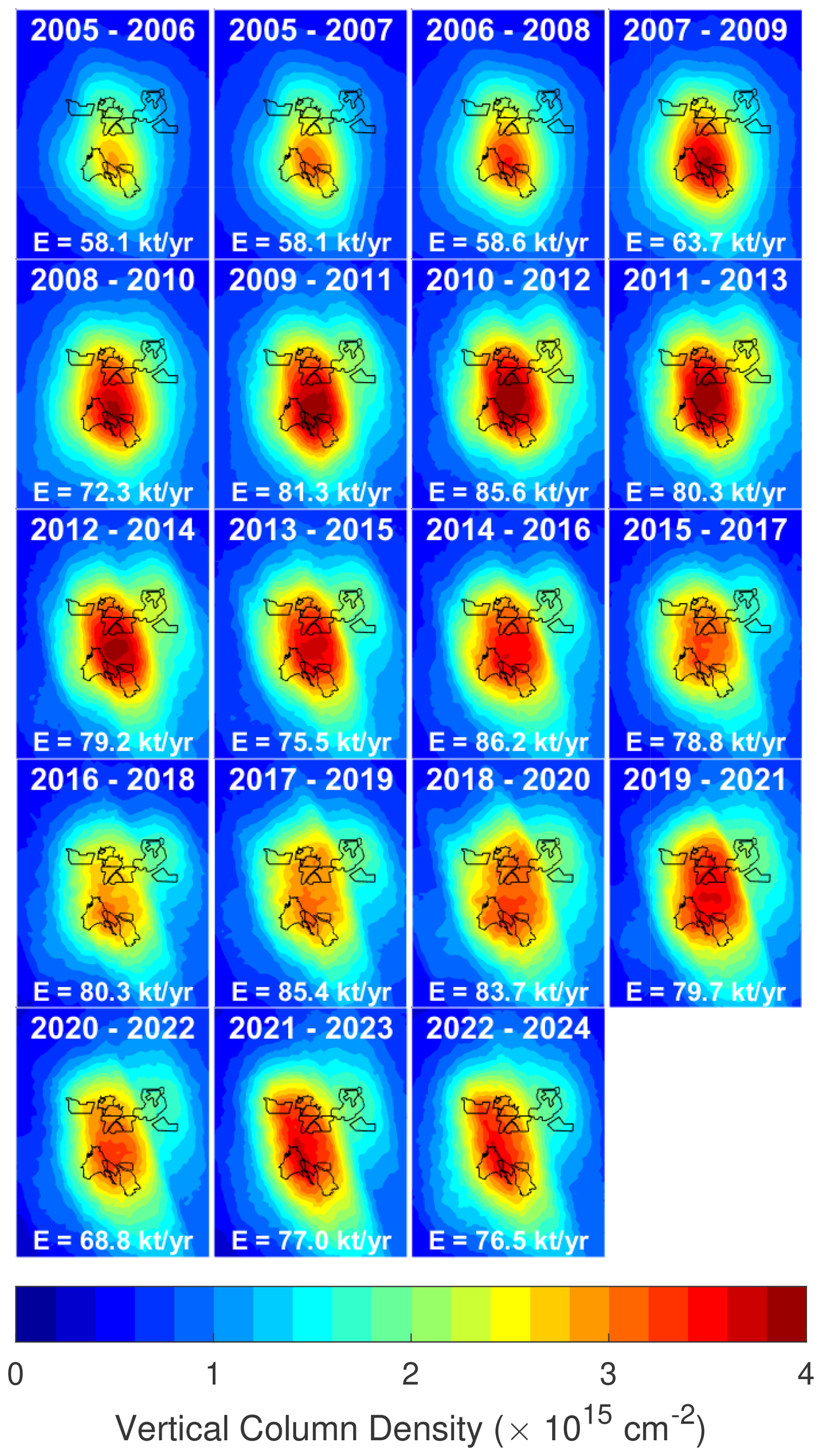
Figure D3 Three-year OMI NO₂ vertical column density (VCD) fit reconstructions over the surface mining, corresponding to the maps in Fig. D2. An averaging radius of 12 km was used. The OMI-derived total NO_x emissions are indicated.

Appendix E: Emissions calculations

Over the course of the OMI mission, a blockage known as the row anomaly has meant an (generally) expanding number of pixels become unreliable, leading to a reduction in data density. It is for this reason that data are analyzed in 3-year periods as opposed to 1 year. Figure E1a shows the impact of the row anomaly on observations within 80 km of the reference location (57.1° N, 111.6° W). Due to variations in solar zenith angle and cloud cover, OMI does not sample evenly through the year. This variation is illustrated in Fig. E1b, with each year generally following this same average pattern. There is uneven sampling throughout the year with few data in November–January due to low sun angles and a drop in the summer due to increased cloud cover.

As a result of this uneven sampling, intra-annual changes in emissions may not be totally captured. To estimate this effect, monthly totals of bitumen mines (Alberta Energy Regulator, 2023a), which should be a good proxy for NO_x emissions, were examined. From Fig. E2, monthly values fluctuate about the annual mean by roughly 10 %–15 %.

A correction factor to account for this unequal sampling throughout the year was used. A monthly total bitumen-mined value was assigned to each OMI pixel (used in the emissions calculations), according to its month and year. For each year, the ratio of the mean monthly bitumen-mined value to the average (over all OMI pixels) of the OMI-sampled bitumen-mined value was computed. This ratio was found to vary from 1.00 to 1.05. It was then used to scale the retrieved emissions in Figs. 9 and 10 and Table E1. These values are smaller than those derived for OMI SO₂ (McLinden et al., 2020) as coverage for NO₂ is less seasonally dependent.

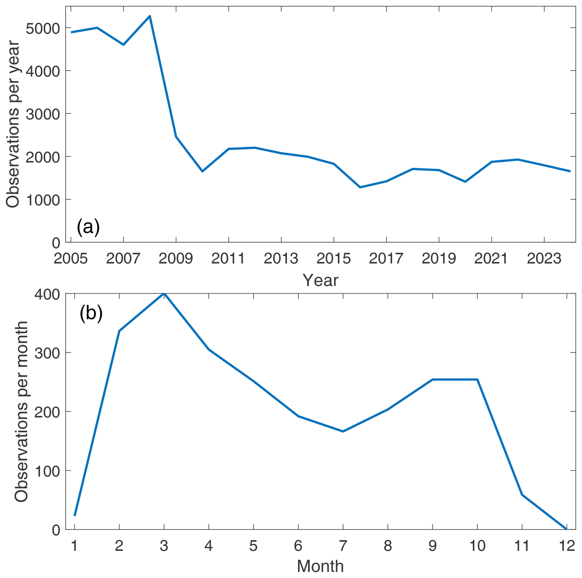
Figure E1 OMI pixels within 80 km of the reference location used in the emissions calculations: (a) total number per year and (b) average number of OMI pixels (per month).

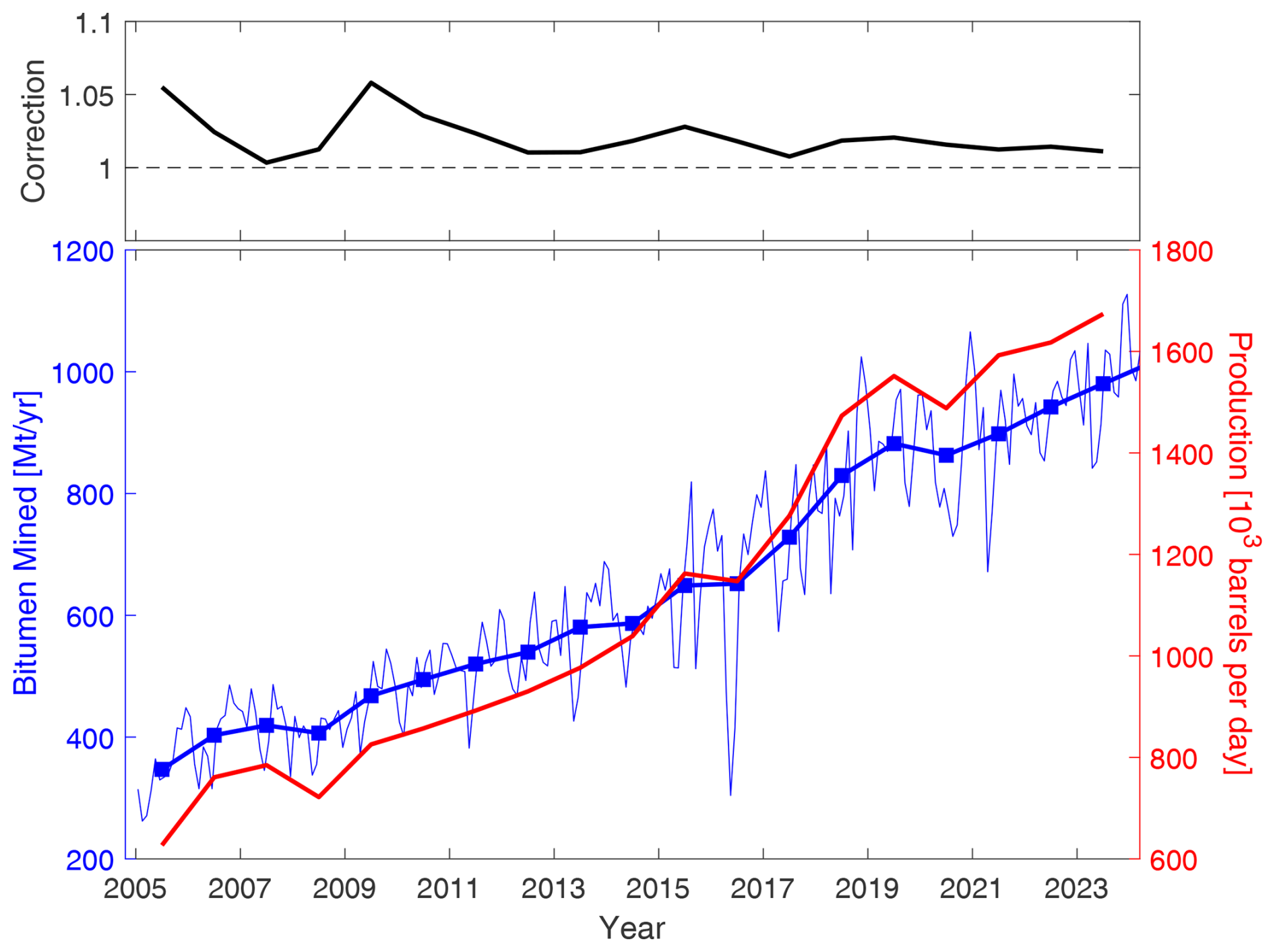
Figure E2 Total monthly and annual bitumen mined from the surface mining region and total production of synthetic crude from the surface mines. (The monthly bitumen mined has been converted to annual rates.) The panel at the top shows the correction factor applied to the annual emissions to account for the monthly sampling.

Table E1 Summary of emissions calculations employing algorithm variants. Emissions given here are averages over the entire 2005–2024 OMI period. Average NPRI stack emissions (2005–2023) are 30.5 kt [NO₂ yr⁻¹]. The mean over all methods, and the variability among methods, is given in the bottom row.

As discussed in Sect. 2.4.3, the missing component of NO_x, NO, is accounted for using an externally derived NO₂ $/$ NO_x ratio. Figure E3 shows a comparison of observed ratios made during the 2018 aircraft campaign in which plumes were tracked downwind of the surface mines. An evolution is observed from values around 0.6 to 0.75 due to photochemical processing. These observations can be compared to the emissions-based method of estimating NO₂ $/$ NO_x, which accounts for the downwind effect, appropriate for annual and June–July time periods, with the latter done to be more consistent with the observations time period. The good overall consistency suggests the emissions-based approach is reasonable. Further, an estimate of uncertainty is derived by looking at the variability.

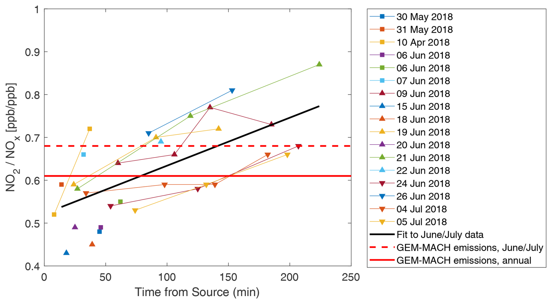
Figure E3 Comparison of NO₂–NO_x ratios. Data from 8 flights in June and July 2018 taken during the oil sands aircraft campaign as a function of time downwind of the source, along with a fit. For comparison, the red lines show the values using the emissions-based approach (see Sect. 2.4.3) based on GEM-MACH-model-simulated OMI data. The standard deviation of the aircraft data about the line of best fit is 0.07, or 11 %.

Emissions calculations were carried out using the point source and several different variants of the multi-source methods. The purpose was to test different assumptions as well as to conduct a sensitivity study that could be used to help quantify uncertainties. A summary of the various emission runs is provided in Table E1.

Seven runs were used: the point source method and six multi-source variants. Variables changed for the multi-source runs included: fitting all emissions using the gridded and mine-specific approach, fitting only fleet emissions (with point source emissions specified) using the gridded and mine-specific approach, and fitting only fleet emissions using the gridded and mine-specific approach but using higher-altitude winds for the stack emissions and lower-altitude winds for the fleet. As can be seen from Table E1 there is little difference among them.

Appendix F: Resolution and the width parameter, σ

The relationship between σ, σ_diff, σ_size, and σ_pixel was explored in Appendix F using a simple model in which a collection of true-Gaussian plume point sources were used to simulate a near-point source (of some radius σ_size) and smoothed to satellite resolution (for pixel size σ_pixel). Fitting the combined distribution to an EMG allowed a relationship between these various terms to be established. Figure F1 shows σ has a behaviour reminiscent of ${\mathit{\sigma }}_{\mathrm{size}}^{\mathrm{2}}$ and ${\mathit{\sigma }}_{\mathrm{pixel}}^{\mathrm{2}}$ and for small values of both values less than 1 km, which suggests σ_diff is small. Figure F1 will be used below to help interpret results.

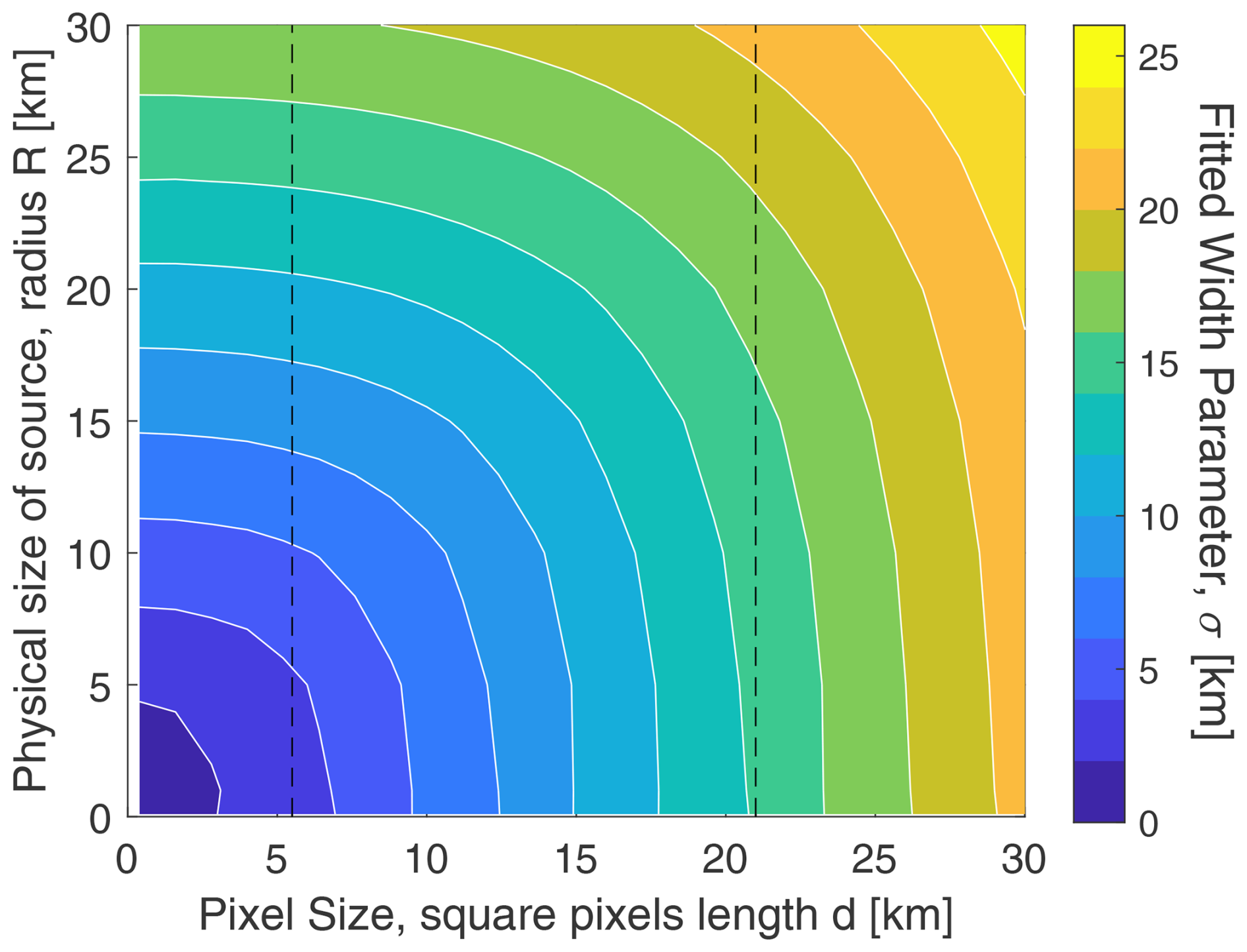
Figure F1 The relationship between the EMG width parameter, σ, and the physical extent of the emissions source and the satellite spatial resolution. See text for information on how this figure was derived. The vertical lines correspond to effective pixel sizes for the OMI and TROPOMI instruments, at 21 and 5.5 km, respectively.

The behaviour of the fitted width parameter, σ, is further examined here in an attempt to understand how it varies with the spatial size or extent of the source, σ_size; satellite pixel size, σ_pixel; and the plume diffusion term, σ_diff. To do this, a set of numerical experiments were performed in which a collection of true-Gaussian plume point sources were used to simulate a near-point source (of some radius σ_size) and smoothed to satellite resolution (for pixel size σ_pixel). The Gaussian plume is of the form given in Stockie (2011) (with α=0.33 km, β=0.86) but integrated in the vertical to simulate VCDs. Each Gaussian was sampled at high spatial resolution, 0.1 km, and the composite distribution was calculated by summing over all Gaussian plumes. This was smoothed to coarser resolutions in order to simulate observations from satellite instruments.

An EMG was then fit to the resultant distribution in order to derive σ. By varying σ_size and σ_pixel, Fig. F1 is derived, which shows a behaviour consistent with Eq. (1). For the smallest case explored, σ_size=0.1 km and σ_pixel=0.4 km, a σ of 0.35 km was found. This can be interpreted as representing the diffusion term and confirms, at least for the EMG formulation, that it is small on this scale. Given this, the form,

$$\begin{array}{}\text{(F1)}& {\mathit{\sigma }}^{\mathrm{2}}=a+b\cdot {\mathit{\sigma }}_{\mathrm{pixel}}^{\mathrm{2}}+c\cdot {\mathit{\sigma }}_{\mathrm{size}}^{\mathrm{2}},\end{array}$$

with a=0.33 km², b=0.41, and c=0.28, is a good representation of the domain considered here. Interestingly, as σ_pixel was defined as a length of a square and σ_size as a radius, their weights are roughly equal when area is considered.

According to Fig. F1 and with the effective pixel size of OMI (as defined as the square root of the average pixel area) being about 20 km, a σ of 15 km is expected. From Sect. 3.2, OMI views a point source with σ=11 km, a value close to but slightly smaller than the 13 km from this numerical experiment. The difference could be related to the fact OMI pixels are not square (as assumed here), and also there is a considerable amount of oversampling by using multiple years of observations.

In the context of this multi-source method, an estimate of the minimum separation distance required to resolve between neighbouring emissions can be estimated by considering their basis functions. The criterion adopted here is that emissions from neighbouring sources can be found as long as the correlation between their basis functions does not exceed 0.5. Using this, the minimum distance between sources as a function of lifetime, τ, and width parameter, σ, is shown in Fig. F2. For OMI, this suggests sources ∼ 22 km apart can be resolved. If a more relaxed threshold of 0.7 is used, then this decreases to about 15.5 km. Wind is also important: if the winds are halved, there is less overlap of the plumes, and 20 km is required; likewise, doubling the wind speed increases this to 24 km. Note that while this suggests low wind speeds are advantageous, in reality this also means the plumes are not as evident, making an accurate emissions calculation more difficult.

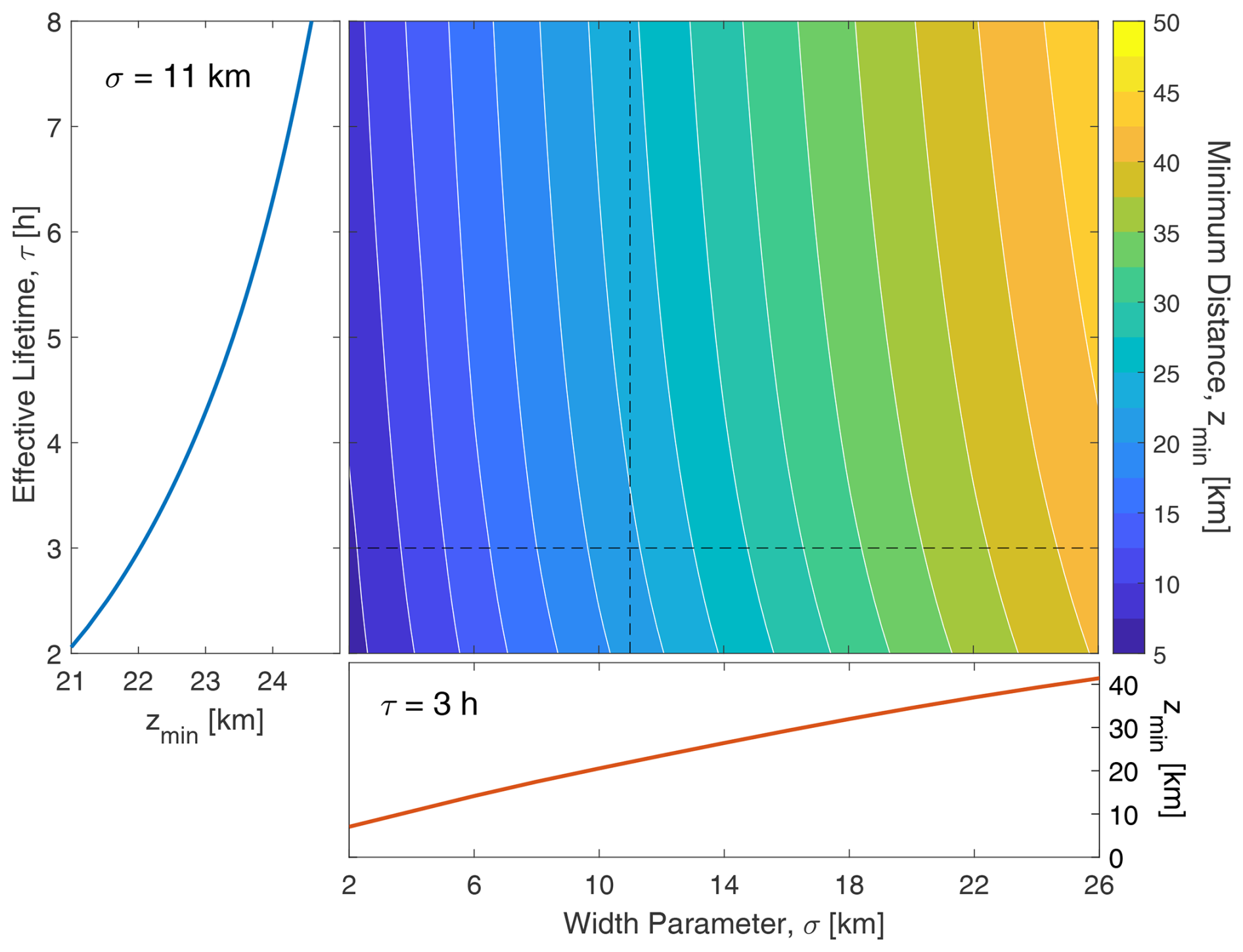
Figure F2 Minimum distance required to distinguish between two point sources as a function of plume width and effective lifetime. The line plots to the left and below show this quantity for σ=11 km and τ=3 h, respectively, and are cross-sections indicated by the dashed white line.

TROPOMI, with its significantly improved spatial resolution relative to OMI (a 12-fold improvement in area, or 3–4-fold improvement in distance), will mean much smaller values for σ and hence an improved ability to resolve emissions.

Figure F3 Comparison of reported and OMI-derived NO_x emissions derived for individual mining operations considering the years 2010–2023, colour-coded according to proximity the their nearest neighbour.

Even though emissions from the multi-source method were simply summed to a total over all surface mining based on a minimum separation distance of OMI of about 22 km, it is nonetheless worth attempting to resolve them. Here we consider the approach in which one source is assigned to each mine (e.g. see Fig. 8) and consider the period 2010–2023 where reported emissions are available for both stack and fleet sources. A scatter plot of the facility-specific emissions is shown in Fig. F3.

For distances between mines of less than about 12 km, with one exception, OMI has difficulty distinguishing between neighbouring sources and can misassign emissions. The two larger emission sources, Syncrude Mildred Lake and Suncor, each with reported emissions of about 20 kt [NO₂] yr⁻¹, are resolved fairly well. Even though Suncor is only about 7 km from its nearest neighbour, it also emits an order of magnitude more NO_x. Overall OMI does show some limited ability to resolve emissions between neighbouring mines. This may suggest that a correlation threshold of 0.5 is too stringent and that perhaps a value of 0.7, which leads to a minimum separation distance of 17 km, is more reasonable.