Numerical case study of the aerosol–cloud interactions in warm boundary layer clouds over the eastern North Atlantic with an interactive chemistry module

The presence of warm boundary layer stratiform clouds over the eastern North Atlantic (ENA) region is commonly influenced by the Azores High, especially during the summer season. To investigate comprehensive aerosol–cloud interactions, this study employs the Weather Research and Forecasting model coupled with a chemistry component (WRF-Chem), incorporating aerosol chemical components that are relevant to the formation of cloud condensation nuclei (CCN) and accounting for aerosol spatiotemporal variation. This study focuses on aerosol indirect effects, particularly the long-range transport of aerosols, in the ENA region under three different weather regimes: a ridge with a surface high-pressure system, a post-trough with a surface high-pressure system, and a weak trough. The WRF-Chem simulations conducted at a near-large-eddy scale offer valuable insights into the model's performance, especially in terms of its ability to use high spatial resolution to capture mesoscale cloud features across various weather regimes. Our result shows that introducing 5 times more aerosols to either non-precipitating or precipitating clouds significantly increases ambient CCN numbers, resulting in, to varying degrees, higher liquid water path (LWP) values. The substantial aerosol–cloud interaction especially occurs in the precipitating clouds and demonstrates the susceptibility of the LWP to changes in CCN under different regimes. Conversely, thin, non-rain clouds at the edges of a cloud system are prone to evaporation, exhibiting an aerosol drying effect. The aerosols released during this process transition back to the accumulation mode, facilitating future activation. This dynamic behavior is not adequately represented in prescribed-aerosol simulations.

1 Introduction

Low-level stratiform clouds are predominantly generated over oceanic regions and are categorized into three main types: warm boundary layer stratiform clouds located on the eastern side of oceanic subtropical highs, stratocumulus clouds that develop over warm western boundary currents during winter cold outbreaks, and Arctic stratus (Klein and Hartmann, 1993). Warm boundary layer stratocumulus clouds, on average, blanket around 20 % of the Earth's surface annually (Wood, 2012; Warren et al., 1988). Their influence on the Earth's energy balance is substantial, primarily through their ability to reflect incoming solar radiation, resulting in significant shortwave cloud radiative effects and, thus, leading to a pronounced negative net radiative effect (Chen et al., 2000; Stephens and Greenwald, 1991; Hartmann et al., 1992).

Research on aerosol–cloud interactions in warm boundary layer clouds has been ongoing since the 1970s. Twomey (1974) proposed that aerosols play an important role in influencing the Earth's energy budget by serving as cloud condensation nuclei (CCN). These CCN are crucial for cloud formation. A higher concentration of CCN results in the formation of clouds with a greater number of smaller-sized cloud droplets (Twomey, 1991). These smaller droplets enhance cloud albedo, known as the first indirect effect, and inhibit precipitation formation while also prolonging cloud lifetime, known as the second indirect effect (Albrecht, 1989). In addition to these indirect effects, aerosol particles have direct, semi-direct, and indirect impacts on the atmosphere's energy budgets and surface, leading to changes in atmospheric stability (Lee et al., 2008). Currently, our understanding of aerosol–cloud interactions remains incomplete. In a recent review paper, Feingold et al. (2024) highlighted that the response of cloud amount (including liquid water content, spatial coverage, and cloud persistence) to aerosol perturbations is still unclear. Both positive and negative adjustments in the liquid water path (LWP) and cloud fraction (CF) have been observed. Increases in cloud amount (positive adjustments) are linked to rain suppression, whereas the enhanced evaporation of smaller droplets and entrainment feedback tend to decrease cloud amount (negative adjustments).

This study focuses on warm boundary layer stratiform clouds located on the eastern side of oceanic subtropical highs, specifically targeting the area over the eastern North Atlantic (ENA) region, where the US Department of Energy (DOE) Atmospheric Radiation Measurement (ARM) program developed a ground-based user facility in the Azores archipelago (Mather and Voyles, 2013). Long-term ground-based observations at the ARM ENA site, aircraft field campaigns near the Azores islands, and satellite retrievals over the ENA region provide comprehensive datasets for observational studies on aerosol–cloud interactions (Zheng et al., 2022, 2024; Ghate et al., 2023; Qiu et al., 2024b).

The presence of stratocumulus clouds over the ENA region is commonly influenced by the Azores High, also known as the Bermuda–Azores High (Rémillard and Tselioudis, 2015). This semipermanent high-pressure system typically develops over the subtropical North Atlantic Ocean. The Azores High often brings stable and relatively dry conditions to the region, which can contribute to the formation and maintenance of stratocumulus clouds. During the summer season, the Azores High tends to strengthen and expand, leading to more persistent high-pressure conditions and often warmer, drier weather in its vicinity. Although synoptic intrusions from high latitudes are less frequent in the summer compared to the winter season (Wood et al., 2015), the ENA region still experiences synoptic variability from weak troughs during the summer months (Mechem et al., 2018; Zheng et al., 2025).

Leveraging the marine boundary layer cloud observations from the ARM ENA observatory, this study aims to study aerosol indirect effects (AIEs), especially the long-range transport of aerosols, in the warm boundary layer clouds over the ENA region under three different synoptic regimes: a ridge with a surface high-pressure system, a post-trough with a surface high-pressure system, and a weak trough (Mechem et al., 2018; Zheng et al., 2025). These regimes are chosen because the ARM site experiences northerly wind conditions during the passage of troughs. This minimizes the influence of the island effect on the observations (Ghate and Cadeddu, 2019; Zheng and Miller, 2022).

Only a few numerical studies have examined aerosol–cloud interactions in marine boundary layer clouds over this region (Zhang et al., 2021; Wang et al., 2020; Kazemirad and Miller, 2020; Christensen et al., 2024). Wang et al. (2020), for example, used the Weather Research and Forecasting (WRF) model with prescribed CCN profiles to simulate the perturbed long-range-transported aerosol concentration for two different cases of marine boundary layer (MBL) clouds. They concluded that when long-range-transported aerosol plumes penetrate down into the drizzling cloud deck, the simulations show an increase in the marine cloud fractions with larger water content, supporting a positive cloud amount adjustment to CCN perturbations. Christensen et al. (2024) utilized an advanced WRF configuration integrated with a Lagrangian framework to assess the effects of aerosols on developing cloud fields across 10 case study days during the ENA field campaign and got the same conclusion. However, a limitation of these studies is that they do not account for the aerosol composition acting as CCN or the changes in aerosol populations following the cloud evaporation process, even though aerosol wet removal is included in their simulations.

To further investigate the impacts of realistic aerosol chemical components and aerosol spatiotemporal variation in the AIEs, this study adopts the WRF model coupled with a chemistry component (WRF-Chem) to examine the AIEs in the ENA region across different synoptic regimes. A brief description of the observational data, the WRF-Chem model, and the configuration and numerical experiments is given in Sect. 2. Simulated results are discussed in Sect. 3, including model evaluation, model sensitivity tests, and cloud susceptibilities. The discussion and summary are provided in Sect. 4.

2 Methodology

2.1 Observational data

2.1.1 MERRA-2

The Modern-Era Retrospective analysis for Research and Applications, Version 2 (MERRA-2), represents the latest advancement in global atmospheric reanalysis during the satellite era. Produced by NASA's Global Modeling and Assimilation Office (GMAO), it utilizes the Goddard Earth Observing System Model (GEOS, version 5.12.4; Molod et al., 2015). The aerosol species are from the inst3_3d_aer_Nv dataset, which is an instantaneous 3D, 3-hourly data collection in MERRA-2 (Global Modeling and Assimilation Office, 2015). The dataset comprises assimilations of aerosol mixing ratio parameters at a native resolution of 0.5° × 0.625° (latitude × longitude) across 72 model layers, encompassing dust, sea salt, sulfur dioxide (SO₂), sulfate (SO₄), black carbon (BC), and organic carbon (OC). The data are provided every 3 h, beginning at 00:00 UTC. Based on Wang et al. (2020), we also adopt MERRA-2 to drive the WRF-Chem initial and boundary conditions for this study (see Sect. 2.2.2 for details).

2.1.2 Geostationary satellite retrievals (Meteosat)

Cloud properties are derived from the Spinning Enhanced Visible and Infrared Imager (SEVIRI) on Meteosat-10 and Meteosat-11, which offer a spatial resolution of 3 km at nadir and a half-hourly temporal resolution over the ENA region. These SEVIRI cloud products are generated using the Satellite ClOud and Radiation Property retrieval System (SatCORPS) algorithms (Painemal et al., 2021). These methods, developed by the Clouds and the Earth's Radiant Energy System (CERES) project, are specifically tailored to support ARM ground-based observation sites (Minnis et al., 2011, 2021). Specifically, this study adopts the cloud fraction for all clouds as the observational reference over the ENA region. The adopted data have been specifically processed (e.g., solar zenith angle, cloud optical thickness, and cloud labels) and averaged to 25 km × 25 km (Qiu et al., 2024b).

2.1.3 Aircraft observation

The US DOE ARM Aerosol and Cloud Experiments in the Eastern North Atlantic (ACE-ENA) aircraft field campaign near the Azores islands provided extensive observations of the vertical distributions of aerosol and cloud properties (Wang et al., 2022). Intensive operational periods (IOPs) of the ACE-ENA took place in late June–July 2017 and January–February 2018. During the 2017 summer IOP, the ARM Aerial Facility (AAF) Gulfstream-159 (G-1) aircraft delivered precise measurements of aerosol size distribution, total aerosol number concentration, and chemical constituents both below and above cloud layers. The SO₄ and OC mass concentrations were measured using the Aerodyne high-resolution time-of-flight aerosol mass spectrometer (HR-ToF-AMS), while refractory BC was measured by the single-particle soot photometer (SP2). Detailed information about each instrument is available on the ARM website (https://www.arm.gov/research/campaigns/aaf2017ace-ena, last access: 11 June 2025). In this study, aircraft measurements of SO₄, OC, and BC from 19 July 2017 are utilized to assess the simulated aerosol vertical profile. However, uncertainties arising from the measurements and spatiotemporal sampling strategies may hinder direct comparisons of absolute values between the observations and modeled results.

2.1.4 ARM ground-based observations

The DOE ARM ground-based instruments deployed on Graciosa Island in the Azores archipelago provide comprehensive measurement of aerosols, clouds, radiation, the atmospheric boundary layer, and other atmospheric properties. In this study, the LWP is retrieved from the brightness temperature measured by a microwave radiometer (MWR) at 23.8 and 31.4 GHz (Liljegren et al., 2001) and used for model evaluation. The temperature and moisture profiles are from the interpolated sonde data, derived from the radiosonde measurement.

2.2 The model

2.2.1 WRF-Chem

The Weather Research and Forecasting (WRF) model (version 4.4.2; Skamarock et al., 2021) coupled with a chemistry component (WRF-Chem; Grell et al., 2005) is used in this study. Standard WRF-Chem permits the simulation of the combined direct, indirect, and semi-direct effects of aerosols (Grell et al., 2005; Fast et al., 2006; Chapman et al., 2009). WRF-Chem version 4.4.2 has sophisticated packages to represent chemistry processes (i.e., gas-phase reaction, gas-to-particle conversion, coagulation, etc.) and aerosol size and composition (Binkowski and Shankar, 1995). In this study, the Regional Acid Deposition Model version 2 (RADM2) photochemical mechanism (Stockwell et al., 1997) is integrated alongside the Modal Aerosol Dynamics Model for Europe (MADE) and the Secondary Organic Aerosol Model (SORGAM) (Ackermann et al., 1998; Schell et al., 2001) to simulate atmospheric chemistry and the evolution of anthropogenic aerosols. MADE/SORGAM adopts a modal approach to represent the aerosol size distribution, predicting mass and number concentrations across three aerosol modes (Aitken, accumulation, and coarse). MADE/SORGAM has inorganic, organic, and secondary organic aerosols and contains aerosol formation processes, including nucleation, condensation, and coagulation. WRF-Chem tracks the number of particles and the mass of chemical compounds (e.g., SO${}_{\mathrm{4}}^{\mathrm{2}-}$, NH${}_{\mathrm{4}}^{+}$, NO${}_{\mathrm{3}}^{-}$, Na⁺, and Cl⁻) in each aerosol mode, including both interstitial aerosols and aerosols present in liquid water (the sum of cloud and rain), as prognostic variables.

The size, composition, and mixing state of aerosols significantly influence their capability to activate as CCN (Zaveri et al., 2010). A physically based aerosol activation parameterization scheme has been developed for climate models to simulate the CCN concentration accurately and efficiently (Abdul-Razzak and Ghan, 2000). This aerosol activation parameterization was initially designed for a single aerosol type with a lognormal size distribution. Then, they expanded this parameterization to accommodate multiple externally mixed lognormal modes, with each mode consisting of both soluble and insoluble materials internally mixed. However, the WRF-Chem (MADE/SORGAM) chemistry package adopts this global internal-mixing assumption, where all particles within a lognormal mode within the same grid cell are instantly combined, resulting in the same chemical composition. This instantaneous internal-mixing assumption modifies the optical and chemical characteristics of particles in WRF-Chem simulations, potentially impacting aerosol–cloud interactions, such as aerosol activation as CCN (Zhang et al., 2014).

2.2.2 The configuration

Our focus in this study is to examine aerosol–cloud interactions close to the scale of large-eddy simulation (LES) over the ARM ENA site. We use WRF-Chem with a full chemistry package involving sophisticated gaseous and aqueous chemical processing calculations and dry and wet deposition. The numerical simulations are employed with four domains consisting of four horizontal resolutions of 5, 1.67, 0.56, and 0.19 km, respectively (Fig. 1), with one-way nesting. There are 550 × 530 grids for d01, 451 × 430 grids for d02, 553 × 532 grids for d03, and 553 × 532 grids for d04. The domain size of domain 4 is about 1°, which is similar to the spatial resolution of global climate models. A total of 75 vertically staggered layers are stretched to have a higher resolution near the surface based on a terrain-following pressure coordinate system. With this setup, the model has roughly 24 model layers in the boundary layer (∼ 2000 m). The time step is 30 and 10 s for advection and physics calculation for domains 1 and 2, respectively. The nesting inner domains 3 and 4 have a time step of 3 and 1 s, respectively. The physics schemes adopted in the simulations are listed in Table 1. The initial and boundary meteorological conditions are taken from ERA5, developed by the Copernicus Climate Change Service (C3S) at the ECMWF (European Centre for Medium-Range Weather Forecasting), the fifth-generation ECMWF atmospheric reanalysis, spanning from January 1940 to the present day (Hersbach et al., 2023). This comprehensive dataset offers hourly estimates of numerous atmospheric, land, and oceanic climate variables, covering the entirety of Earth on a 31 km grid. The atmospheric component is resolved using 137 levels, spanning from the surface up to 80 km in height.

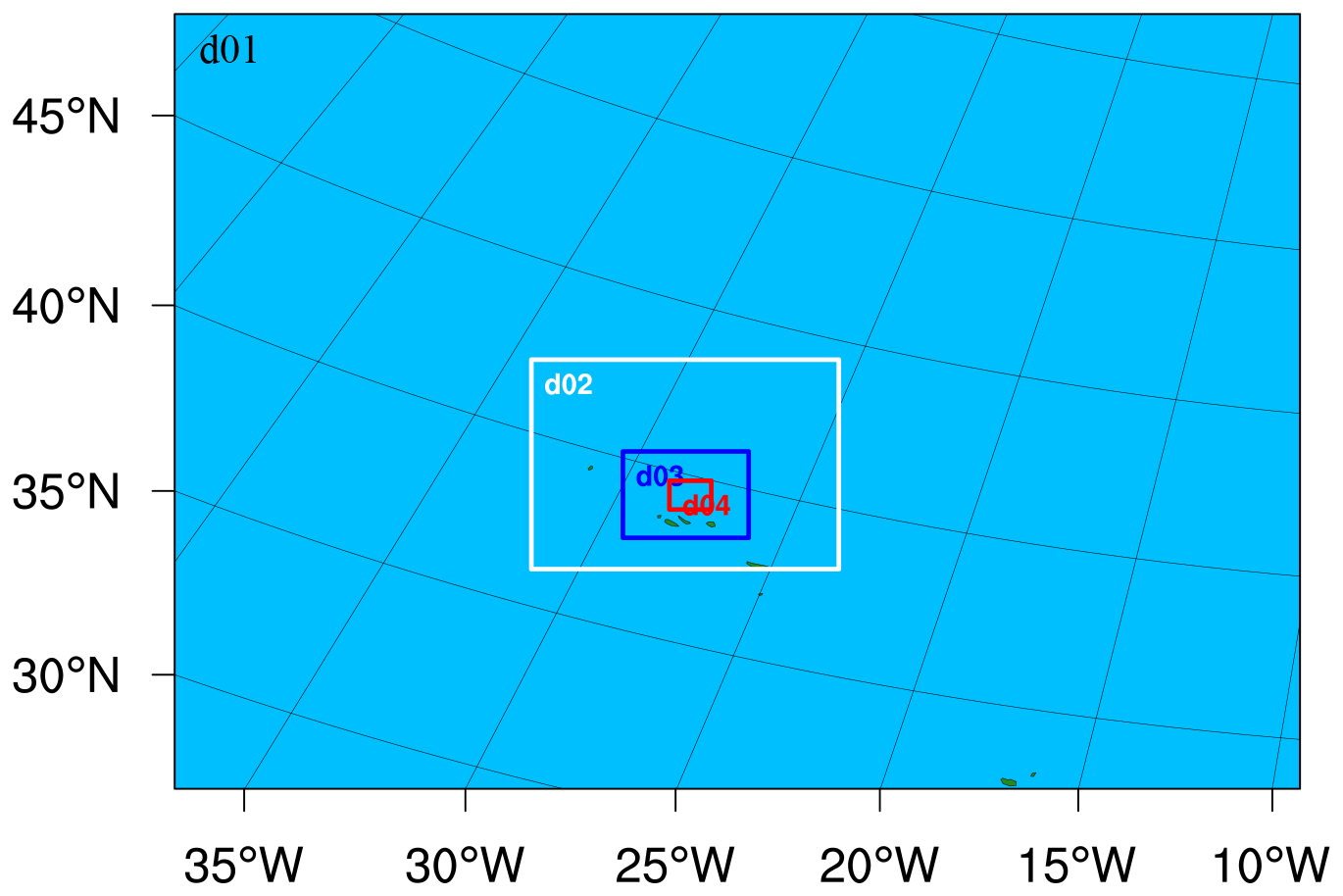
Figure 1 The model domains designed for the simulations. The four domains denote four horizontal resolutions of 5 km (d01), 1.67 km (d02), 0.56 km (d03), and 0.19 km (d04), respectively.

Table 1 The WRF physics scheme configuration.

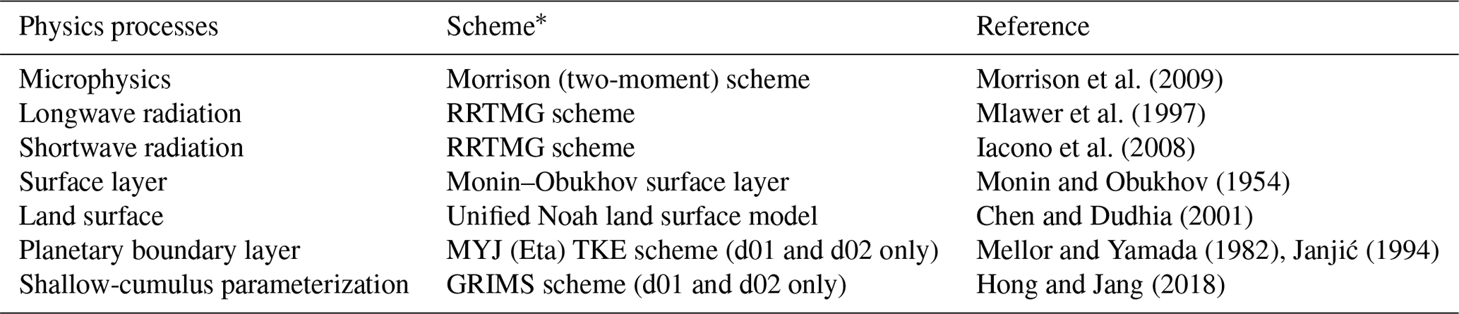
^* The abbreviations/acronyms used are as follows: RRTMG – Rapid Radiative Transfer Model for General Circulation Models; MYJ – Mellor–Yamada–Janjic; TKE – turbulent kinetic energy; GRIMS – Global/Regional Integrated Modeling System.

The computational expense of conducting a four-domain WRF-Chem simulation, particularly with LES resolution, is exceedingly high. To mitigate this, we execute WRF solely for the two outer domains (d01 and d02), leveraging the WRF downscaling module (ndown) (Skamarock et al., 2008) to generate meteorological initial and boundary conditions for domain 3. As a result, we only need to perform WRF-Chem simulations for the two inner domains (d03 and d04), leading to an almost 50 % reduction in total computational cost (compared to the original four-domain run, which had a throughput of 4 h d⁻¹ using 1080 cores). It is important to note that a high temporal frequency for domain-3 boundary conditions is essential due to its fine horizontal resolution (0.56 km). In this context, we update the boundary condition every 5 min for domain 3.

To enhance the realism of aerosol mass simulation in remote marine regions, such as the ENA site, we account for major aerosol species (BC, OC, and SO₄) and SO₂ from MERRA-2 in the boundary conditions of domain 3. Aerosols in the initial condition are introduced into the restart file (wrfrst) following a 1 h initial run, rather than in the initial condition file (wrfinput), to address certain numerical challenges. According to the emission setup for MADE/SORGAM, we assume that the Aitken mode and the accumulation mode account for 20 % and 80 % of the aerosol mass (BC and OC), respectively (Tuccella et al., 2012). Conversely, for SO₄, 80 % is allocated to the Aitken mode and 20 % to the accumulation mode, reflecting the faster growth rate of SO₄ and a longer duration of growth from the domain-3 boundary. Because MERRA-2 only provides aerosol mass, the aerosol number concentrations for different aerosol species are estimated with the density assumption of BC (1.7 g cm⁻³), OC (1.0 g cm⁻³), and SO₄ (1.77 g cm⁻³) based on Liu et al. (2012). Aerosol optical depth retrieved from satellite remote sensing can offer valuable information for comparison; however, it may be subject to high bias in our study cases due to cloud cover.

It is common to consider that the ENA region is an unpolluted area, as it is far away from anthropogenic pollution sources. Besides the long-range transport of aerosols, two local aerosol sources, dimethyl sulfide (DMS) and sea salts, are also important for the aerosol budget. Kazil et al. (2011) pointed out that the observed DMS flux from the ocean in the VOCALS-REx field campaign over the southeastern Pacific can support a nucleation source of aerosol. DMS oxidation by nitrate (NO₃) produces SO₂ and then increases the SO₄ concentration (Toon et al., 1987). As we adapted the SO₂ and SO₄ concentration from MERRA-2 in the initial and boundary conditions, we did not double-count DMS emissions in our simulations. As a result, chemical species emissions, except for sea salt, are excluded from the simulations. The emission of sea salt particles is parameterized using the method outlined by Clarke et al. (2006) in WRF-Chem. Sea salt emissions are driven by surface wind speed. The simulated surface wind speed aligns closely with ERA5 data; however, the sea salt concentration is only one-third of the value found in the MERRA-2 analysis. To improve the alignment with the sea salt aerosol concentration observed in the MERRA-2 reanalysis, we adjust the parameter factor for sea salt emissions to 3 times the original estimate (further comparison can be found in Sect. 3).

2.3 Study cases and numerical experiment design

We select three specific study cases to assess the impact of the long-range transport of aerosols on warm boundary layer clouds, with each case representing a typical meteorological regime observed over the ENA site. The first case, dated 1 July 2016, exhibits the formation of overcast stratocumulus clouds (Fig. 2a) within a meteorological regime characterized by a ridge system in the free troposphere and a high-pressure system near the surface (Fig. 2d). Predominant northwesterly and northerly winds in the area of the ARM ENA site coincide with the presence of long-range-transported aerosols, commonly found along the periphery of the surface high-pressure system (Logan et al., 2014; Gallo et al., 2023).

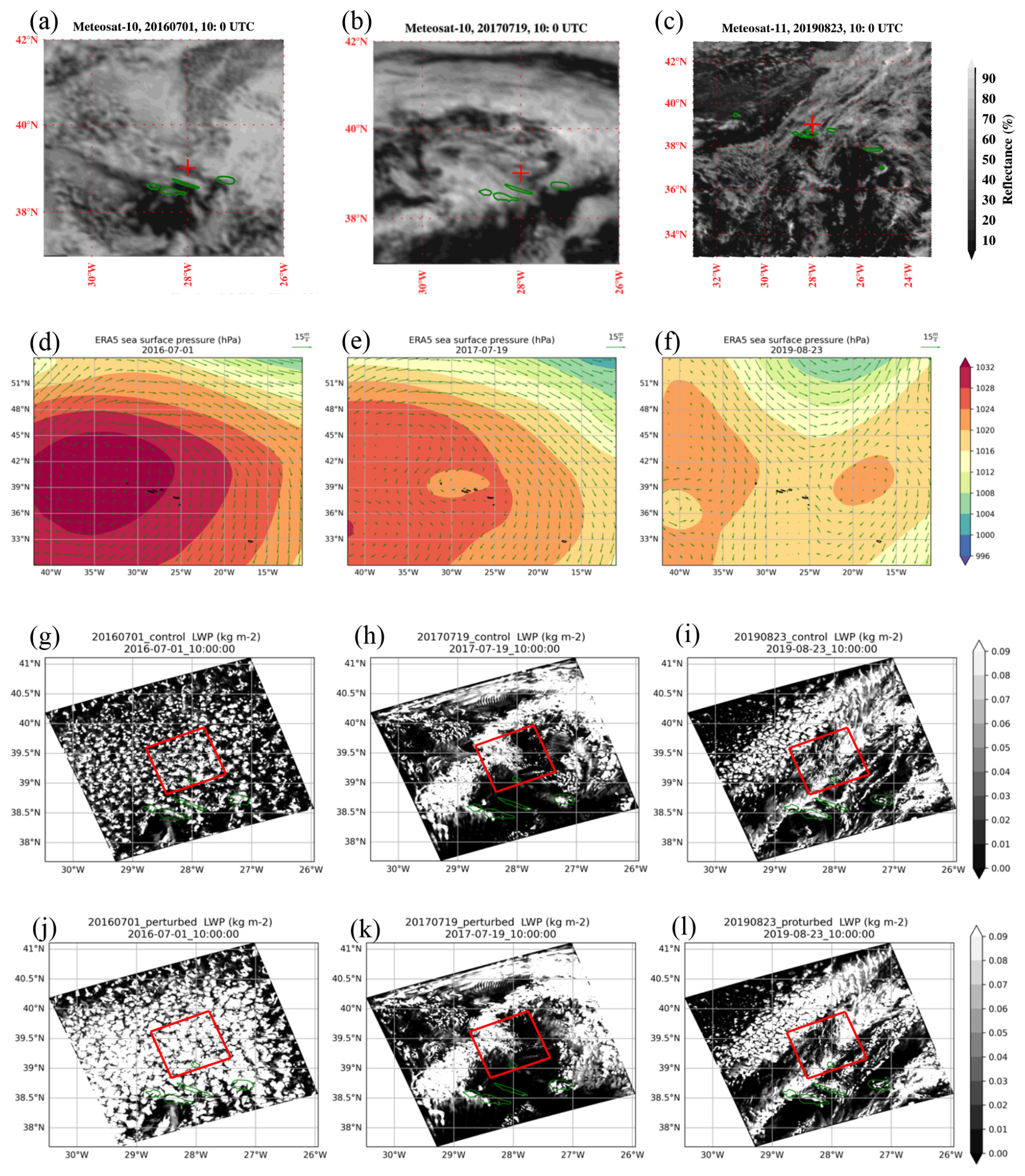
Figure 2 Spinning Enhanced Visible Infrared Imager (SEVIRI) images from the Meteosat satellite at 10:00 UTC on (a) 1 July 2016, (b) 19 July 2017, and (c) 23 August 2019 over the ENA. Panels (d), (e), and (f) depict the same days as panels (a), (b), and (c), respectively, but for the ERA5 mean sea surface pressure (contour; units: hPa) and 10 m surface wind (arrow; units: m s⁻¹). Panels (g), (h), and (i) depict the same days as panels (a), (b), and (c), respectively, but for the WRF-Chem-simulated liquid water path (LWP; units: kg m⁻²) in the control runs, while panels (j), (k), and (l) show the perturbed runs. The red boxes in the panels indicate the result from domain 4.

The second case on 19 July 2017 is a stratocumulus cloud case (Fig. 2b) within a post-trough regime featuring a surface high-pressure system under the influence of a trough system (Fig. 2e). Following the trough passage, robust northwesterly winds facilitated the influx of long-range-transported aerosols into the region; these winds then shifted to northerly winds as the trough moved away. Because the ACE-ENA aircraft field campaign intensive operations period (IOP) was during this time, aircraft aerosol observational data can be used to evaluate the model performance for this case.

Finally, the third case, dated 23 August 2019, occurred during a period of weak-trough activity (Fig. 2f). Here, we noted the presence of broken, thicker stratocumulus clouds, often accompanied by deeper cloud formations (Fig. 2c). Long-range-transported aerosols were again observed, primarily carried by northwesterly and northerly winds, albeit with weaker surface wind speeds compared to the preceding two cases.

All simulations start at 12:00 UTC on the preceding day of the study case, spanning a duration of 36 h, with the initial 12 h dedicated to spin-up. Again, aerosols in the initial condition are introduced into the restart file after a 1 h initial run (i.e., 13:00 UTC). The three aforementioned cases, labeled as control cases (20160701_control, 20170719_control, and 20190823_control), are utilized to examine the behavior of warm boundary layer clouds under diverse meteorological conditions. Additionally, we formulated three perturbed cases (20160701_perturbed, 20170719_perturbed, and 20190823_perturbed) by amplifying aerosol concentrations in both the initial and boundary conditions and the sea salt emissions by a factor of 5 relative to each control case. These control cases represent clean conditions, with near-surface CCN concentrations below 100 cm⁻³, at the ARM ENA site. A comparison between the control and perturbed cases elucidates the sensitivity of warm boundary layer clouds to aerosol enhancements under varying meteorological conditions, thereby contributing to a deeper understanding of cloud microphysics processes under varying atmospheric dynamics.

3 Results

3.1 Model evaluation

3.1.1 Meteorological conditions

Figure 2g, h, and i display the model-simulated LWP in the control runs over domains 3 and 4. The modeled LWP is the calculated in-cloud LWP only. The simulations with a fine spatial resolution effectively capture synoptic frontal systems and cloud features, particularly when compared to the cloud images from the Meteosat satellite (Fig. 2a, b, and c). Thin, uniform stratocumulus clouds on 1 July 2016 are simulated in 20160701_control, while the solid stratocumulus and frontal system on 19 July 2017 are also well captured in 20170719_control. Broken stratocumulus clouds on 23 August 2019 are reproduced in the simulation of 20190823_control. Figure 2j, k, and l display the model-simulated LWP in the perturbed runs. The overcast stratocumulus clouds are simulated better in 20160701_perturbed (Fig. 2j), which more accurately reflects reality.

The control runs serve as a basis for comparing the boundary layer structure against the interpolated soundings obtained from the ARM ENA site. Figure 3 depicts the comparison, showing the simulated air temperature aligning closely with the observed values. However, on 1 July 2016, the model (20160701_control) displays a warm bias with respect to capturing the temperature inversion (Fig. 3a and b), with the simulated inversion layer situated approximately 200–300 m lower than observed during the whole study period. Potential temperature and relative humidity show consistent performance, as illustrated in Figs. S1b and S2b in the Supplement, respectively. While the model indicates high relative humidity (> 90 %) within 1000 m, observations show this extending up to ∼ 1200 m.

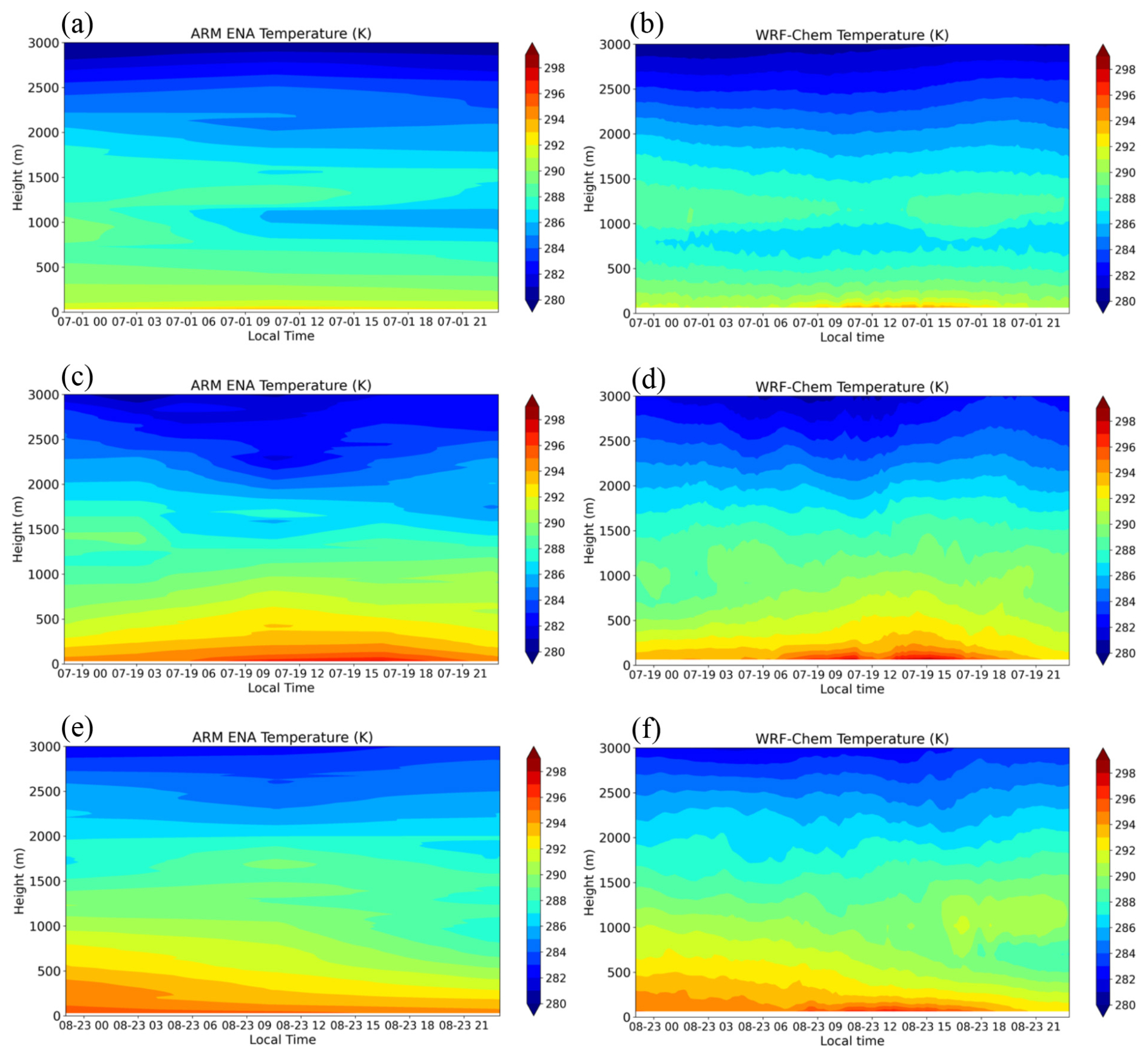
Figure 3 The time series (local time; UTC−1) of temperature profiles (units: K) from ARM-interpolated soundings at the Azores (39.09° N, 28.02° W) on (a) 1 July 2016, (c) 19 July 2017, and (e) 23 August 2019. Panels (b), (d), and (f) depict the same dates as panels (a), (c), and (e), respectively, but show the average temperature from WRF-Chem-simulated results over 20 × 20 grids centered on the Azores (at an approximate 4 km resolution).

For the 19 July 2017 case, the model (20170719_control) successfully represents the diurnal cycle of the temperature vertical gradient within 1000 m height. However, compared to observations, the model does not catch the inversion at 1500 m height near noontime and shows a warm bias in the model's simulated temperature (Fig. 3c and d). The model simulation also tends to depict drier conditions in the evening compared to the observation (Fig. S3c and d).

On 23 August 2019, characterized by a weak-trough regime and higher boundary layer height, the simulation of 20190823_control accurately captures warm and moist air advection in the morning but has difficulty maintaining fidelity in the late afternoon. Notably, the lower troposphere becomes excessively warm and dry after 17Z local time compared to observations (Figs. 3e, 3f, S2e, S2f, S3e, and S3f).

In general, all simulations effectively capture large-scale conditions and cloud features (Fig. 2) across different synoptic regimes but do not accurately represent temperature inversions and air advection patterns. Discrepancies are noted in the simulated boundary layer height, which is lower, and the inversion is weaker than actual observations. Furthermore, the discrepancies tend to increase in the later stage of simulation.

3.1.2 Aerosol evolution

As mentioned in Sect. 2.2.2, we incorporate major aerosol species (BC, OC, and SO₄), from MERRA-2 into the domain-3 initial (in the restart file at 13:00 UTC) and boundary conditions to enhance the realism of aerosol simulation. Figure 4 shows time-series SO₄ vertical profiles from both MERRA-2 and WRF-Chem for three study cases. Here, we demonstrate the time evolution of SO₄. This species is the main aerosol component among the three introduced aerosol species, about 60 %–80 % of total aerosol mass, in the initial conditions.

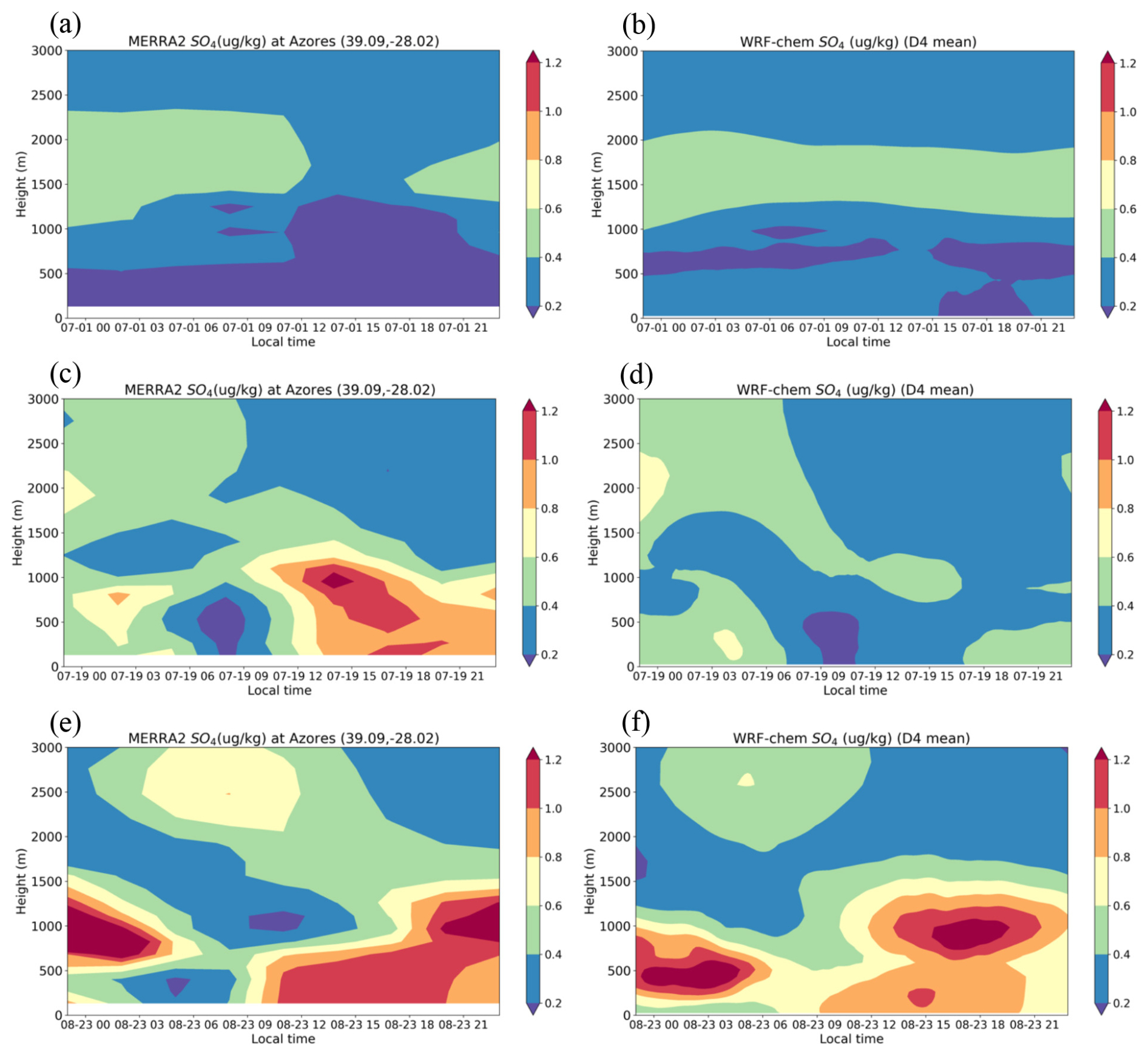
Figure 4 The time series (local time; UTC−1) of SO₄ profiles (units: µg kg⁻¹) from MERRA-2 at the Azores (39.09° N, 28.02° W) on (a) 1 July 2016, (c) 19 July 2017, and (e) 23 August 2019. Panels (b), (d), and (f) depict the same dates as panels (a), (c), and (e), respectively, but show the average aerosol concentration from WRF-Chem-simulated data over domain 4.

Compared to the MERRA-2 data, 20160701_control well captures the long-range-transported SO₄ between 1000 and 2000 m, which is above the cloud deck, on 1 July 2016 (Fig. 4a and b). Moreover, the observed high BC and OC are concentrated in this layer (Figs. S4a and S5a), as are simulated high BC and OC (Figs. S4b and S5b). Figures 4c and e show two MERRA-2 time-series vertical distributions of SO₄ on 19 July 2017 and 23 August 2019, with both showing low-altitude (below 1500 m) aerosol plumes. On 19 July 2017, the concentrations of BC and OC showed two peaks: one near the surface and another above 1500 m in the free troposphere (Figs. S4c and S5c). This pattern indicates the presence of a biomass-burning signature in the plume on that day (Wang et al., 2020). However, the simulation of 20170719_control did not capture the near-surface BC, OC, and SO₄ concentration after 11Z on 19 July 2017 (Figs. S4d, S5d, and 4d). This is because, in the case of the post-tough regime, the wind direction changed from northwesterly to northerly when the trough moved away, and the aerosol plume in domain 3 did not propagate into domain 4 when the wind direction changed (figure not shown). Nevertheless, the simulation of 20170719_control still captures the BC and OC plumes in the free troposphere (above 2000 m height) (Figs. S4d and S5d).

Aircraft observations during ACE-ENA provide more accurate depictions of the aerosol vertical distribution and aerosol layer heights, with differentiation of aerosol type. Figure 5a shows the vertical distribution of aerosol mass concentrations averaged over the flights on 19 July 2017. BC, OC, and SO₄ all increase with height above clouds (∼ 1000 m), indicating downward propagation of aerosol plumes and possible interaction with MBL clouds (600–1000 m). Here, we also see high SO₄ in the free troposphere, similar to MERRA-2, but the model underestimates the OC concentration in the free troposphere. On the other hand, within the MBL, there is a much higher concentration of SO₄ in the MBL than those of BC and OC in the observations. This phenomenon is also captured by the WRF-Chem simulation (Fig. 5b), but the model did not capture the magnitude of the SO₄ concentration.

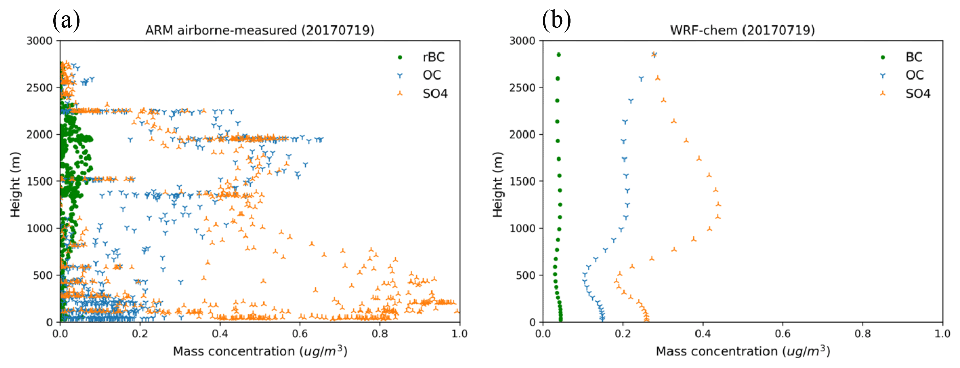
Figure 5 (a) ARM airborne-measured vertical profiles of SO₄, OC, and the refractory BC (rBC) mass concentration (units: µg cm⁻³) averaged over multiple flights on 19 July 2017. Note the highly uncertain and noisy aerosol observations between 600 and 1000 m height due to cloud contamination. (b) WRF-Chem-simulated vertical profile of SO₄, OC, and the BC mass concentration (units: µg cm⁻³) averaged over domain 4 during the flight time from 08:40 to 11:50 UTC.

Similarly, for the case of 20190823, within the low boundary layer, there is a much higher concentration of SO₄ in the low boundary layer (Fig. 4e). After noontime on 23 August 2019, BC and OC show both high-altitude plumes and low-altitude plumes approaching into the domain, potentially indicating two different aerosol sources (Figs. S4e and S5e). Again, while the simulation of 20190823_control well captures the time evolution of aerosol plume, the boundary of high-altitude plumes and low-altitude plumes appears 300 m lower in the simulations (∼ 600 m in altitude; Figs. S4f and S5f) compared to the observations (∼ 900 m in altitude).

Sea salt particles serve as an important source of CCN over the ocean, particularly under unpolluted conditions. However, due to their larger particle size, sea salt particles tend to accumulate near the ocean surface and are swiftly removed by dry deposition and sedimentation processes (Chin et al., 2002). The simulation of 20160701_control (Fig. S6a and b) accurately reproduces sea salt concentrations, with respect to both magnitude and vertical distribution, consistent with observations, same as the case of 20170719 (Fig. S6c and d). Nevertheless, the model encounters difficulties with respect to simulating sea salt concentrations for the case of 23 August 2019 (Fig. S5e and f), corresponding to a weak-trough system (Fig. 2c). Although the simulated surface wind speed matches well with ERA5 (Fig. S7), the underestimation of sea salt concentrations may be attributed to limitations in the emission parameterization, which is overly reliant on surface wind speed (Gong, 2003).

3.1.3 Cloud properties

In Fig. 6, we observe a comparison between the simulated results and observations of the LWP and CF at different spatial scales (4 km and domain-averaged resolutions, respectively) to leverage the spatiotemporal advantages offered by both sets of observations. The ARM ground-based instrument recorded an LWP of over 400 g m⁻² during the nighttime with drizzle droplets reaching to the surface on 1 July 2016 (Fig. 6a). At sunrise (around 6Z local time), the LWP decreases to a range of about 100 g m⁻² and then increases again to 600 g m⁻² after 21Z.

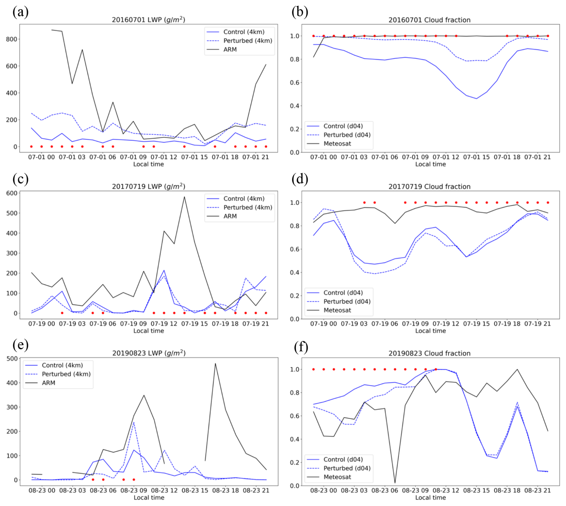
Figure 6 Panels (a), (c), and (e) are the hourly time series (local time; UTC−1) of the 4 km averaged (4 km) liquid water path (units: g m⁻²) simulated from the WRF-Chem control case (solid blue line), the WRF-Chem perturbed case (dashed blue line), and observed from ARM (solid black line) on 1 July 2016, 19 July 2017, and 23 August 2019, respectively. Panels (b), (d), and (f) are the hourly time series of the domain-averaged (d04) cloud fraction simulated from the WRF-Chem control case (solid blue line), the WRF-Chem perturbed case (dashed blue line), and observed from Meteosat (solid black line) on 1 July 2016, 19 July 2017, and 23 August 2019, respectively. The 4 km averaged data are averaged from the model-simulated results over 20 × 20 grids centered on the Azores (at an approximate 4 km resolution). The red dots indicate when the rainfall intensity is higher than 0.001 (0.01) mm h⁻¹ in a 4 km averaged area (or domain 4).

For comparison with the ARM ground-based observations, the WRF-Chem-simulated result is averaged over 20 × 20 grids centered on the Azores, corresponding to an approximate resolution of 4 km (Fig. 6a). Overall, the control run generates a thin cloud layer with an underestimated LWP during the nighttime, capturing only 10 %–20 % of the observed LWP. The simulated clouds are more consistent with the observations during the daytime, especially in the perturbed run. However, it is important to note that the LWP retrieved by MWR experiences significant uncertainties under drizzling or precipitating conditions. This is primarily due to the scattering effects of large raindrops and raindrops accumulating on the instrument's radome, which can result in an overestimation of the LWP (Tian et al., 2019; Cadeddu et al., 2020).

Figure 6b depicts the comparison of the CF between observations and WRF-Chem. The CF values obtained from Meteosat are close to 1, indicating a solid cloud field. In contrast, the CF simulated by 20160701_control range between 0.5 and 0.9 on a domain-averaged scale. Similar to the LWP results, the simulated CFs from 20160701_control exhibit a diurnal cycle, with higher values during the nighttime and lower values during the daytime. Due to the thinner clouds simulated in 20160701_control based on the LWP, the modeled CF is 40 %–60 % lower than the observation in the afternoon, indicating that clouds dissipate more quickly in the control run. Conversely, the 20160701_perturbed scenario demonstrates improved performance in both the LWP and CF. This indicates that the 20160701 case is sensitive to aerosol variations, with the CCN number being too low in the control run.

Compared to a ridge system like the case of 20160701, the WRF-Chem model has difficulty capturing the warm boundary layer clouds under a regime characterized by a post-trough system (20170719) or a weak-trough system (20190823). Compared to the observations, the simulated LWP in 20170719_control is about 30 % of the observed value (Fig. 6c). In contrast, the simulated CF performs better, reaching about 75 % of the observed value (Fig. 6d). The discrepancy between the modeled results and observations may arise from delayed moisture transfer from the outer domain or insufficient vertical resolution. In this instance, the cloud systems move quickly under the post-trough weather regime. A 5 min moisture input from the boundary condition using WRF downscaling (ndown) may not be sufficient to transport moisture into the inner domain, making it difficult for the model to develop thicker marine stratocumulus clouds, especially for such high spatial resolution. On the other hand, in another ongoing project, we increased the vertical layers to 99, which doubles vertical layers below 2 km. However, the test with 99 levels only slightly improves the cloud cover and LWP. The estimated LWP susceptibility shows little to no change. The insignificant improvement indicates that even higher resolution is needed to fully simulate the cloud processes near the sharp boundary layer inversion for these solid stratocumulus cloud layer. Another possible reason is that the sixth-order horizontal diffusion used in the study (diff_6th_opt = 2) rapidly dissipates marine stratiform clouds, especially at the high spatial resolution (Knievel et al., 2007). It is worth noting that Christensen et al. (2024) conducted sensitivity tests using various shallow-cumulus and microphysics schemes, and the different combinations of these schemes had a substantial impact on the simulated cloud amount as well.

Moving to the case of 20190823, overall, compared to the observations, the control run captures the LWP and CF slightly better, especially at the domain-averaged scale (Fig. 6e and f). Based on the LWP observed from ARM, there are two systems passing in the area: one between 5 and 13Z and the other between 17 and 22Z on 23 August 2019 (high ARM LWP in Fig. 6e). The simulation of 20190823_control captures the first system but slightly underestimates the LWP; however, the model misses the second system. The model simulated CFs also match well with Meteosat (Fig. 6f). Only after 17Z, the model misses catching the second system. The CFs drop 50 %–70 % compared to the observations.

The underestimation of the LWP and CF in model simulations leads to insufficient longwave cooling at the cloud top. This reduced cooling weakens cloud-top entrainment, resulting in a less pronounced boundary layer inversion and a shallower boundary layer height (identified in Sect. 3.1.1). This creates a negative feedback loop, where the initial inaccuracies in cloud properties affect boundary layer dynamics (Zheng et al., 2021). On the other hand, in the perturbed runs, the results show an adjustment in the LWP and CF values, aligning more closely with the observations. This suggests that the CCN number is underestimated in the control runs (more discussion in Sect. 3.3). The model's response to aerosol changes highlights its capability for studying aerosol–cloud interactions.

3.2 Aerosol composition and activation

The advantage of utilizing WRF-Chem to investigate aerosol–cloud interactions stems from its capability to simulate the spatiotemporal distribution of CCN. This modeling is based on various aerosol components and their sizes, as well as their dynamic responses to wet removal processes associated with clouds and precipitation. In traditional simulations that rely on fixed or prescribed aerosol distributions, accurately representing these factors can be particularly challenging. WRF-Chem, however, allows for a more nuanced understanding by dynamically modeling how aerosol populations evolve over time, especially after cloud evaporation processes. During the evaporation process, the reduction in cloud water can lead to a re-entrainment of aerosols back into the atmosphere, altering their concentration and properties. This change can affect subsequent cloud formation and precipitation patterns, highlighting the importance of capturing these interactions for reliable predictions.

In this section, we concentrate on aerosol activation, considering its size and chemical composition across three different cases. The following section will discuss the aerosol indirect effect and how changes in cloud properties feedback into the aerosol population and its activation capability.

In Fig. 7a, the solid blue line and dashed blue line represent the vertical profiles of total aerosol number concentration (including the Aitken mode and accumulation mode) and the aerosol number concentration of the Aitken mode, respectively. These profiles are averaged over domain 4 on 1 July 2016. The environment shown in the figure is characterized as clean, with a total aerosol number concentration below the cloud top (approximately 1000 m in height) measuring less than 300 cm⁻³. In the 20160701_control simulation, the total aerosol number is low, and approximately 70 % of the total aerosol numbers belong to the Aitken mode. According to the study conducted by McCoy et al. (2024), who utilized aerosol number concentration measurements from ARM airborne observations on 15 July 2017, it was found that the ratio of the Aitken mode to the total aerosol number was approximately 50 %–60 % within an altitude of 1000 m. Compared to this observational analysis, our simulations generate an overabundance of small-sized aerosols, which result in a low concentration of CCN. This discrepancy arises from the assumptions made when constructing the aerosol initial and boundary conditions (80 % for Aitken-mode and 20 % for accumulation-mode SO₄).

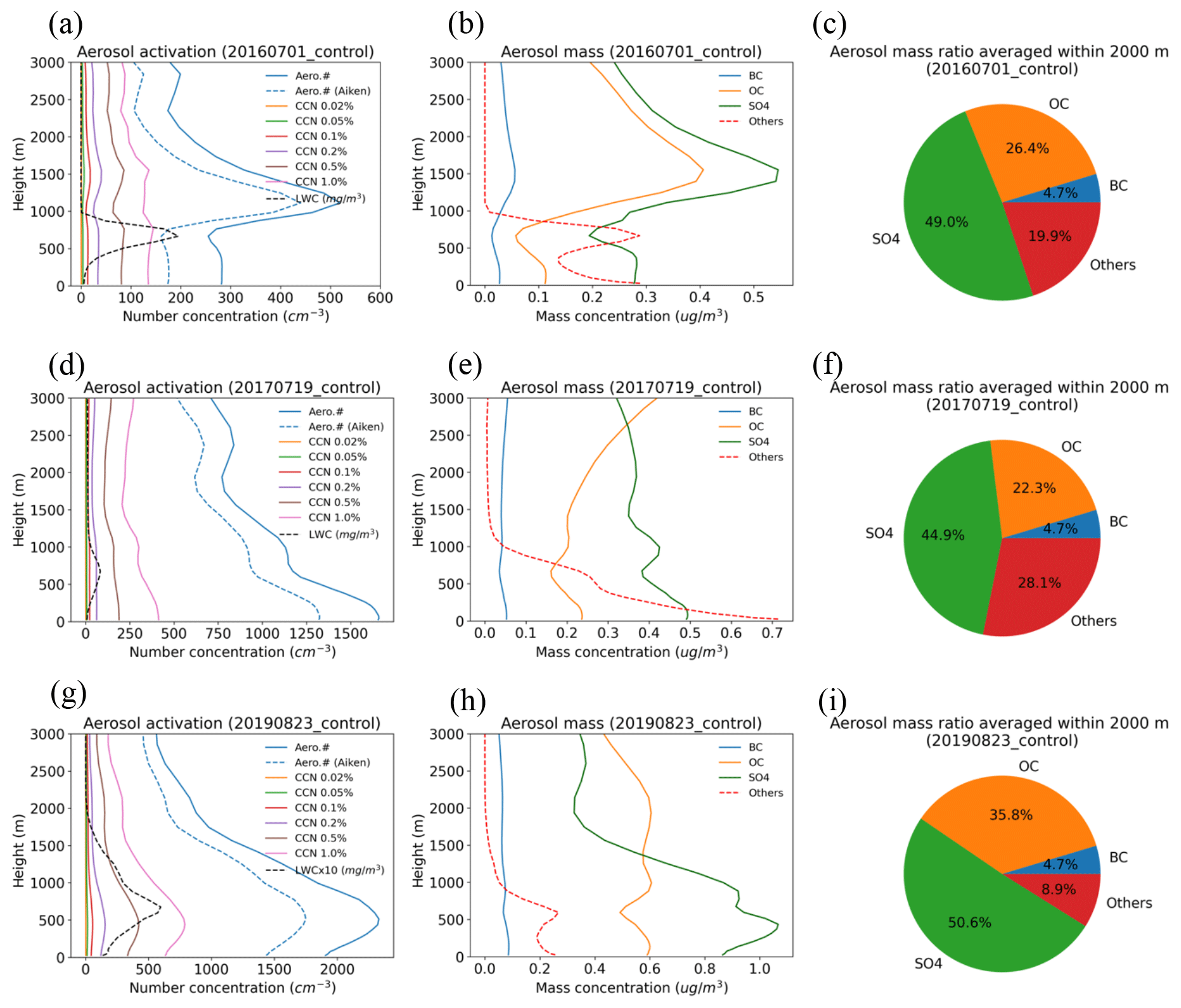
Figure 7 Panels (a), (d), and (g) are the WRF-Chem vertical profiles of aerosol number concentration (Aitken mode and accumulation mode; units: cm⁻³), aerosol number concentration (Aitken mode only; units: cm⁻³), CCN number concentration below different supersaturations (units: cm⁻³), and liquid water content (LWC; cloud and rain; units: mg m⁻³) averaged over domain 4 on 1 July 2016, 19 July 2017, and 23 August 2019, respectively, in the control runs. Panels (b), (e), and (h) are the WRF-Chem vertical profiles of BC, OC, SO₄, and other species (like sea salt) (units: µg cm⁻³) averaged over domain 4 on 1 July 2016, 19 July 2017, and 23 August 2019, respectively, in the control runs. Panels (c), (f), and (i) present pie charts of the aerosol mass of different species averaged within 2000 m height on 1 July 2016, 19 July 2017, and 23 August 2019, respectively, in the control runs. Note that the LWC is adjusted to fit the scale of the x axis for each case.

The CCN calculation presented in Fig. 7a is based on the Köhler theory, which considers both the aerosol size (curvature effect) and the chemical composition (solution effect) to estimate the theoretical CCN number concentration at different supersaturations. Below 1.0 % supersaturation, the CCN number concentration is found to be 42 % of the total aerosol number (could be estimated from 100 % of accumulation mode and 16 % of Aitken mode) (Fig. S8a). In the simulation of 20160701_control, the CCN number concentration below 0.2 % (0.5 %) supersaturation is only 11 % (25 %) of the total aerosol number, which is lower than the observations reported in Wang et al. (2020), who observed that the CCN number concentration under 0.35 % supersaturation was approximately 25 % of the total aerosol number. Even though SO₄ is the dominant chemical component, accounting for nearly 50 % (as shown in Fig. 8b and c), the presence of an excessive number of Aitken-mode aerosols may be the primary reason for the low activation rate. The curvature effect caused by these Aitken-mode aerosols hinders their ability to act as CCN effectively.

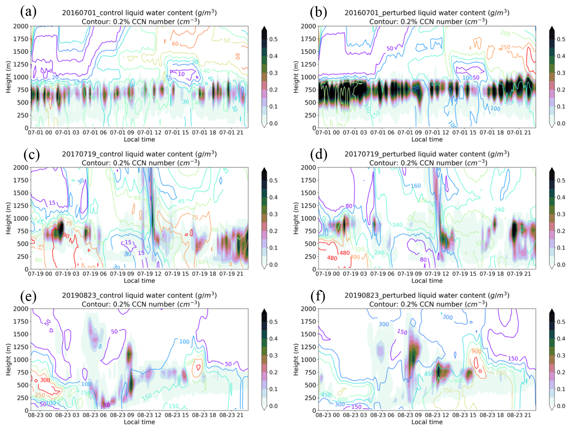
Figure 8 Panels (a), (c), and (e) are the time series (local time; UTC−1) of the 4 km averaged cloud liquid water content profile (shade; units: g cm⁻³) and CCN (0.2 % supersaturation) number concentration profile (contour; units: no. cm⁻³) on 1 July 2016, 19 July 2017, and 23 August 2019, respectively, in the control runs. Panels (b), (d), and (f) are the same as panels (a), (c), and (e), respectively, but for the perturbed runs. The data are averaged from the model-simulated results over 20 × 20 grids centered on the Azores (at an approximate 4 km resolution).

In the simulation of 20170719_control, most aerosols are concentrated within a height of 1000 m, which corresponds to the cloud layer height (Fig. 7d). The average aerosol number concentration across the entire domain is measured to be 1286 cm⁻³ within a height of 2000 m, and the Aitken mode is 80 % of the total aerosol number in this case. The chemical composition of aerosols in the 20170719_control is mainly SO₄, with the other species exhibiting lower concentrations (Fig. 7e and f). This variation in vertical distribution leads to more aerosols being activated under the cloud top at a height of 1500 m. This is attributed to the presence of a peak value of accumulation-mode aerosols and SO₄ at this height.

Because of the high number concentration of simulated Aitken-mode aerosols, overall, the activation rate is low. Below 1.0 % supersaturation, the CCN number concentration is estimated to be 25 % of the total aerosol number. This could be a result of 100 % of the accumulation-mode aerosols and 7 % of the Aitken-mode aerosols contributing to the CCN population (Fig. S8c). The CCN number concentration below 0.2 % (0.5 %) supersaturation is only 4 % (12 %) of the total aerosol number.

Among the three cases studied, the case of 20190823 stands out as the most polluted case, but the aerosol component and vertical distribution are close to the case of 20170719 (Fig. 7c and i). The average aerosol number concentration across the entire domain is measured to be 1850 cm⁻³ within a height of 2000 m. The Aitken-mode aerosols are also high and contribute to more than 75 % of the total aerosol number in this case (Figs. 7g and S8e). The large SO₄ species concentration also leads to more aerosols being activated under the cloud top at a height of 2000 m. The CCN number concentration below 0.2 % (0.5 %) supersaturation is only 6 % (17 %) of the total aerosol number, slightly better than the case of 20170719.

The cloud droplet numbers observed in the three cases fall within the range of CCN numbers below 0.1 % and 0.2 % supersaturation. Therefore, in the subsequent sections, we utilize the CCN number concentration below 0.2 % supersaturation as a representative of the CCN activation rate.

3.3 Cloud responses to aerosol perturbations

Figure 8 illustrates the comparison of time-series profiles of cloud water content (CWC) and CCN number concentration below 0.2 % supersaturation between the control runs and perturbed runs. This figure also demonstrates the CCN spatiotemporal variation in our simulations. Specifically, for the case of 20160701, it is evident that the CWC in 20160701_perturbed exhibits a positive response to increased CCN compared to the CWC in 20160701_control. This result aligns with most WRF studies that use fixed or prescribed CCN numbers to investigate aerosol–cloud interactions (Wang et al., 2020; Christensen et al., 2024).

Echoing the insufficient longwave cooling at the cloud top due to the underestimation of the LWP and CF in model simulations discussed in Sect. 3.1.3, Terai et al. (2014) also observed weak cloud-top entrainment in their study of five pockets of open cells, using aircraft data from the VAMOS Ocean–Cloud–Atmosphere–Land Study Regional Experiment (VOCALS-REx). Their research indicated that clouds tend to break up easily in the absence of aerosols, characteristic of a pristine environment. Consistent with their findings, our study demonstrates that in-cloud collision–coalescence processes effectively remove aerosols, particularly because of the wider range of cloud droplet sizes present in a clean environment (i.e., the control runs) (Table 2). Even in the control run for 20160701, our results indicate that broken open-cell clouds in a pristine environment struggle to develop into closed clouds.

Table 2 The 10 min mean and standard deviation of cloud condensation nuclei (CCN), liquid water path (LWP), cloud droplet number (N_c), cloud radius (R_e), and rainfall intensity (RI) over three study cases. Data are averaged over ∼ 25 km of domain 4, and the total 16 averaged grids are in domain 4. Rain and non-rain are averaged over the grids where the RI on the grid is larger than and equal to zero, respectively. Only CCN are averaged within 1000 m height over domain 4; other variables are averaged within 2000 m height.

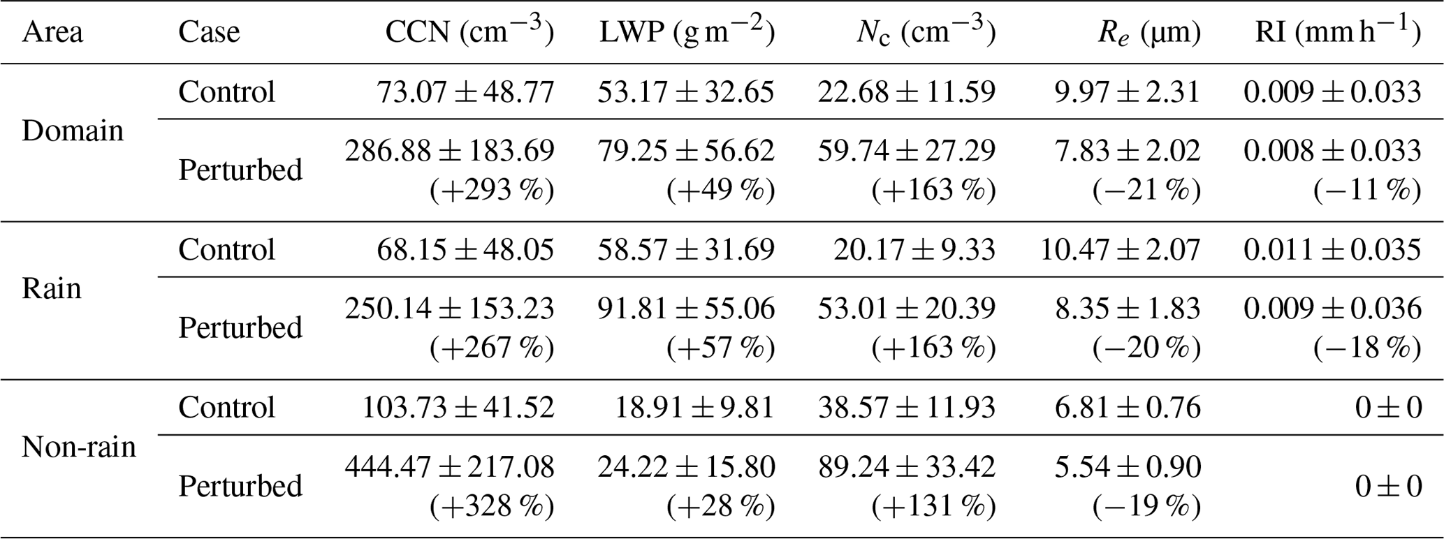
Figure 9a depicts the time series of the domain-averaged LWP, encompassing both cloud and rain, and CCN number concentration below 0.2 % supersaturation for both the 20160701_control and 20160701_perturbed cases. This visualization provides a quantitative representation of the change in CCN number concentration, which increases from a mean value of 32.52 cm⁻³ in the control run to 127.68 cm⁻³ in the perturbed run, approximately 4 times higher than the control run. Because we want to avoid counting high CCN number concentrations above cloud top which do not readily become cloud droplets, the CCN number concentration is averaged from the surface up to the height of 1000 m (Wang et al., 2020).

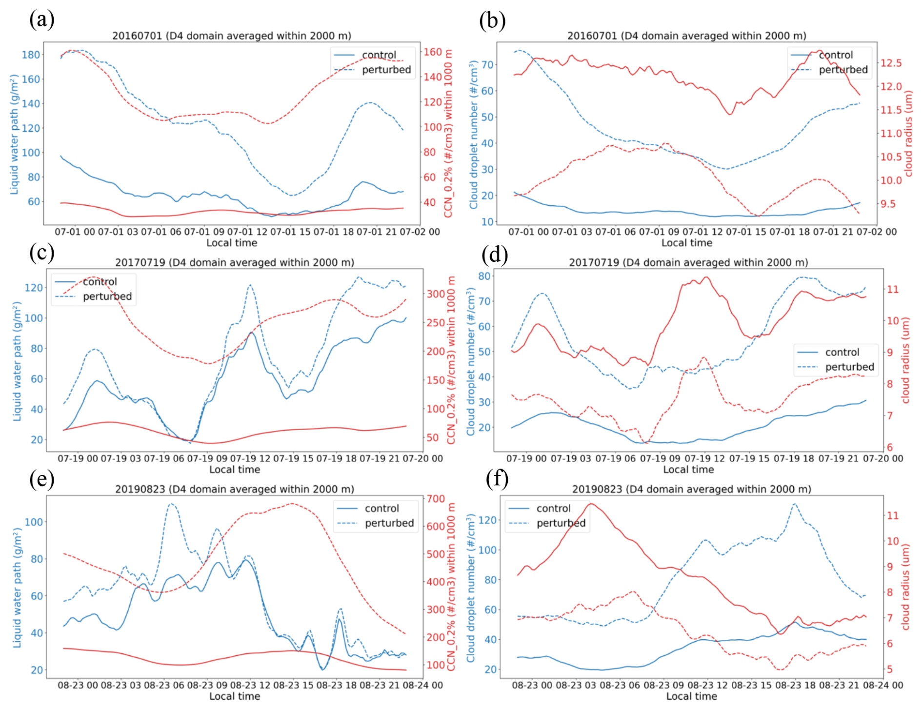
Figure 9 Panels (a), (c), and (e) are the time series of the domain-averaged liquid water path (blue lines; units: g m⁻²) and CCN number concentration below 0.2 % supersaturation (red lines; units: no. cm⁻²) for the control case (solid lines) and the perturbed case (dashed lines) on 1 July 2016, 19 July 2017, and 23 August 2019, respectively. Panels (b), (d), and (f) are the time series of the domain-averaged cloud droplet number (blue lines; units: no. cm⁻³) and cloud radius (red lines; units: µm) for the control case (solid lines) and perturbed case (dashed lines) on 1 July 2016, 19 July 2017, and 23 August 2019, respectively. Only CCN data are averaged within 1000 m height over domain 4; other variables are averaged within 2000 m height.

The LWP in the 20160701_control case exhibits a domain mean value of 64.88 g m⁻², which subsequently increases to 123.27 g m⁻² in the 20160701_perturbed case. As mentioned in Sect. 3.1, the LWP for the 20160701 case follows a diurnal cycle, with higher values during nighttime and lower values during daytime. This diurnal cycle is also observed in the perturbed simulation, with the larger differences in CCN and LWP between the control run and perturbed run during nighttime (Fig. 9a).

After increasing the aerosol concentration, the cloud droplet number in the 20160701_perturbed run demonstrates similar responses. In the 20160701_control case, the domain-averaged value of the cloud droplet number is 14.03 cm⁻³, which subsequently increases to 45.52 cm⁻³ in the 20160701_perturbed case. As the cloud droplet number increases, the cloud radius decreases from 12.23 µm in the control run to 10.08 µm in the perturbed case.

The case of 20170719 represents a post-trough weather regime, and Fig. 8c illustrates the passage of a frontal system in the area after 8Z on that day. In the 20170719_perturbed simulation, the CWC increases following the system's passage (Fig. 8d) compared to the CWC in the 20170719_control run. Additionally, the ambient CCN number in the perturbed run is also higher. The temporal variation in the CCN concentration in Fig. 9c shows elevated CCN numbers before and after the system enters the domain. In the 20170719_control case, the domain-averaged value of the CCN number concentration is 60.51 cm⁻³, which subsequently increases to 253.51 cm⁻³ in the 20170719_perturbed case. The domain-averaged LWP also exhibits an increase, rising from 59.31 g m⁻² in the 20170719_control run to 74.07 g m⁻² in the 20170719_perturbed case. Notably, this change primarily occurs after the passage of the frontal system.

The cloud droplet number consistently shows higher values in the perturbed case (Fig. 9d), and this pattern is similar to the difference in CCN between the two runs of 20170719 (Fig. 9c). In the 20170719_control case, the domain-averaged value of cloud droplet number is 20.70 cm⁻³, whereas this value is 56.09 cm⁻³ in the perturbed case. When the cloud droplet number increases in the perturbed run, the cloud radius decreases from 9.90 µm in the control run to 7.49 µm in the perturbed case. This reduction in cloud radius is even smaller than the cloud radius observed in the case of 20160701.

The case of 20190823 is similar to the case of 20170719, but it represents a weak-trough weather regime. Figure 8e also illustrates the passage of a cloud system in the area between 5 and 17Z on 23 August 2019, and the CWC in the perturbed run increases during this period. Quantitatively, in the 20190823_control case, the domain-averaged value of the CCN number concentration is 124.32 cm⁻³, which subsequently increases to 475.37 cm⁻³ in the 20190823_perturbed case, which is also about 3 times higher. The domain-averaged LWP also exhibits an increase, rising from 48.92 g m⁻² in the 20190823_control run to 58.53 g m⁻² in the 20190823_perturbed case.

Differing from the case of 20170719, the frontal system moved away from the study domain after noontime, and the differences in the CCN number or cloud droplet number between the control and perturbed runs become even more pronounced after the system (Fig. 9e and f). This is because aerosols are transported to the area following the frontal system (Fig. 4f) which in turn activates more aerosols as CCN. In the 20190823_control case, the domain-averaged value of the cloud droplet number is 33.94 cm⁻³, whereas this value is 79.97 cm⁻³ in the perturbed case. When the cloud droplet number increases in the perturbed run, the cloud radius decreases from 8.51 µm in the control run to 6.45 µm in the perturbed case. This reduction in cloud radius is similar to the cloud radius observed in the case of 20170719.

We observe that a large aerosol-induced LWP occurs during the periods of rainfall (Fig. S9). To accurately quantify the differences, we calculate the average LWP over approximately 25 km of domain 4. This results in 16 averaged grids per output file, with each file generated every 10 min. This averaging process is based on Arola et al. (2022) and Zhou and Feingold (2023) to avoid the impact of heterogeneity and co-variability on the results. Specifically, we aggregate the simulation grids with a spatial resolution of approximately 190 m to form a larger grid of around 25 km for each 10 min simulation output, as shown in Fig. S10a.

Table 2 presents the 10 min mean and standard deviation of several variables, including CCN, LWP, cloud droplet number (N_c), cloud radius (R_e), and rainfall intensity (RI), across three study cases. The classification of “rain” and “non-rain” is based on the RI (unit: mm h⁻¹) on the averaged grid. Specifically, a grid is considered to be “rain” if the RI is greater than zero. In the control cases, the averaged CCN number is 73.07 cm⁻³, and the corresponding LWP is 53.17 g m⁻². However, in the perturbed cases, the CCN number increases approximately 3-fold, reaching 218.21 cm⁻³, and the LWP increases by 49 % to 79.25 g m⁻². The introduction of additional aerosols in the perturbed cases also leads to a significant increase in the N_c value, from 22.68 cm⁻³ in the control cases to 59.74 cm⁻³ in the perturbed cases. Consequently, the R_e decreases by 21 %, from 9.97 to 7.83 µm, and the RI decreases by 11 %, from 0.009 to 0.008 mm h⁻¹.

To investigate the interaction between aerosols and clouds, we analyze the results separately for rain and non-rain grids. In both the control and perturbed cases, we observe that the CCN number within 1000 m is lower in the rain grids compared to the non-rain grids, primarily due to the washout effect caused by rainfall. Additionally, the LWP over the rain grids is generally higher than that over the non-rain grids. Furthermore, when comparing the control and perturbed cases, we find that the LWP over the rain grids increases by 57 %, from 58.57 to 91.81 g m⁻². In contrast, the LWP over the non-rain grids only increases by 28 % (Table 2). This difference can be attributed to the conversion of cloud droplets to raindrops through processes like autoconversion and collection, which occurs more prominently over the rain grids. We also observe that, in the non-rain grids, especially at the cloud edges (or low LWP), the perturbed cases reveal an increased presence of small cloud droplets. This abundance of smaller droplets facilitates evaporation, resulting in a reduced LWP (e.g., clouds in the bottom right-hand corner of Fig. S10a and b). Consequently, N_c over the rain grids is lower compared to N_c over the non-rain grids. Moreover, when introducing aerosols in the perturbed runs, the results over the rain grids exhibit larger cloud drops and a wider radius spectrum compared to the results over the non-rain grids. This suggests that the presence of aerosols has a more pronounced effect on cloud properties within the rain grids.

Zheng et al. (2022) conducted a study on the aerosol–cloud interaction using ground-based measurements from the ARM program, focusing on the influence of environmental variables. Their findings revealed that, when there is ample water vapor and low CCN loading, the active coalescence process leads to a broader size distribution of cloud droplets, resulting in an increase in cloud droplet radius. On the other hand, when there is enhanced activation of CCN and condensational growth of cloud droplets due to higher CCN loading below the cloud, the cloud droplet radius decreases. This combined effect signifies an intensified aerosol–cloud interaction, leading to a broad range of cloud droplet radii. The simulated results in our study, specifically over the rain grids where a sufficient water vapor environment is considered, demonstrate a significant aerosol–cloud interaction, where increased CCN introduces more newly converted droplets, resulting in a broad range of cloud droplet radii.

As we utilize a comprehensive aerosol module in WRF-Chem to examine aerosol–cloud interactions, we are able to explore how changes in cloud properties, driven by increased CCN, affect aerosol concentrations. For example, in the post-trough regime (20170917 case) and the weak-trough regime (20190823 case), we observe that the cloud structure exhibits more open-cell stratocumulus clouds (Fig. 2h and i). As mentioned above, the increased number of smaller cloud droplets at the cloud edge facilitate evaporation and results in a lower LWP (Fig. S10). The larger aerosols from the evaporated clouds return to the accumulation mode, making them more likely to activate as CCN again.

To demonstrate how robust this process is on the aerosol–cloud interaction, we calculate a time series of the ratio of the number concentration of CCN at a supersaturation of 0.2 % in the perturbed runs to that in the control runs, normalized by the corresponding accumulation-mode aerosol concentration, defined as ${\left({\text{CCN}}_{\mathrm{0.2}\mathit{\%}}/\text{Accu. aerosols}\right)}_{\mathrm{perturbed}}$ $/$ ${\left({\text{CCN}}_{\mathrm{0.2}\mathit{\%}}/\text{Accu. aerosols}\right)}_{\mathrm{control}}$, shown in Fig. 10. A ratio greater than 1 suggests that accumulation-mode aerosols in the perturbed cases are more readily activated as CCN at a supersaturation of 0.2 %, especially in the cases of 20170719 and 20190823. Conversely, a ratio less than 1 is observed during the first half of the day in the 20160701 case, which is attributed to the very low levels of accumulation-mode aerosols in the model.

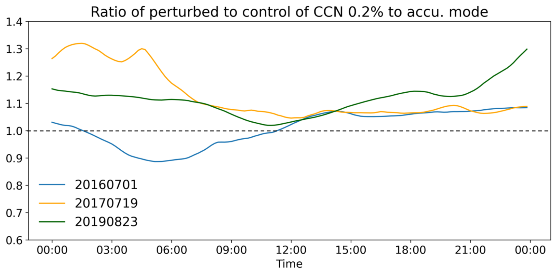
Figure 10 The time series of the ratio of the number concentration of CCN at a supersaturation of 0.2 % in the perturbed runs to that in the control runs, normalized by the corresponding accumulation-mode aerosol concentration, defined as ${\left({\text{CCN}}_{\mathrm{0.2}\mathit{\%}}/\text{Accu. aerosols}\right)}_{\mathrm{perturbed}}$ $/$ ${\left({\text{CCN}}_{\mathrm{0.2}\mathit{\%}}/\text{Accu. aerosols}\right)}_{\mathrm{control}}$. The dashed black line indicates the value of unity.

3.4 Cloud liquid water path (LWP) susceptibilities

In this study, the susceptibility of the LWP to changes in the CCN concentration is quantified using the logarithmic slope between the LWP and CCN, denoted as dln (LWP)/dln (CCN) (Gryspeerdt et al., 2019). This slope represents the sensitivity of the LWP in warm stratocumulus clouds to variations in the CCN concentration, as shown in Fig. S10c. As presented in Table 2, we aggregate the simulation grids with a spatial resolution of approximately 190 m to form a larger grid of around 25 km for each 10 min simulation output. This averaging process helps to reduce the impact of heterogeneity and co-variability on the results.

Figure 11 illustrates the averaged cloud susceptibilities for various LWP and CCN or N_c bins across three study periods. The logarithmic slope between the LWP and CCN is calculated at each output time (every 10 min) using data from 16 aggregated grid points from the control run and 16 aggregated grid points from the perturbed run. Our study reveals that when the CCN concentration is below 100 cm⁻³, the susceptibility for different LWP and CCN values is positive and the values are large, indicating that changes in the LWP are sensitive to variations in the CCN number. Moreover, our work also demonstrates that the AIE is large when an increase in CCN can have a large impact on the LWP enhancement. However, when the mean CCN concentration exceeds 100 cm⁻³, the relationship between the LWP and CCN becomes more complex, with both positive and negative susceptibilities observed. This suggests that the change in LWP is influenced by other factors, such as environmental conditions and cloud precipitation status (as shown in Fig. 11a). Over 70 % of the results meet the criterion of statistical significance (p ≤ 0.01), further supporting the robustness of the observed relationships. It is important to note that the CCN number used in our study is averaged from the surface up to the height of 1000 m, which may introduce uncertainty to the absolute values of susceptibility by including aerosols that are not directly involved in the aerosol–cloud interaction (Wang et al., 2020).

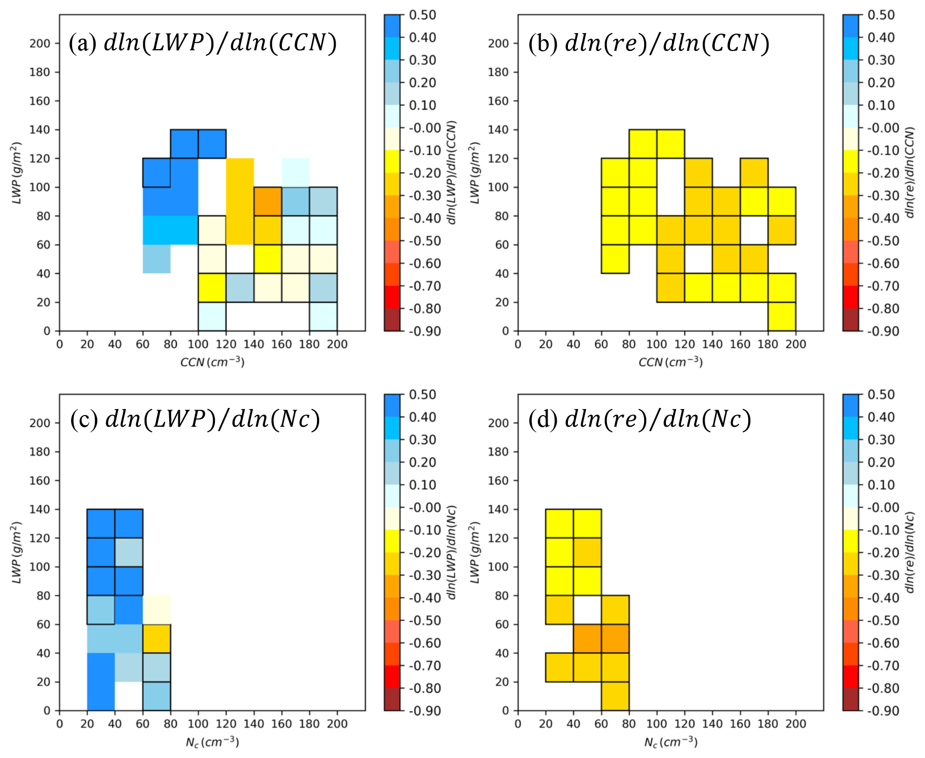
Figure 11 Panels (a) and (b) are the mean liquid water path (LWP) and cloud radius (R_e) susceptibilities for different cloud condensation nuclei (CCN) and LWP bins for three study cases, respectively. Panels (c) and (d) are the same as panels (a) and (b), respectively, but for different cloud droplet number (N_c) and LWP bins. The logarithmic slope between the LWP and CCN, denoted as (dln (LWP)/dln (CCN)), is calculated at each output time (every 10 min) using data from 16 aggregate grid points (∼ 25 km for each grid point) from the control run and 16 aggregated grid points from the perturbed run. Black edges indicate statistically significant results with p ≤ 0.01.

Additionally, our simulations indicate that the N_c in this study is generally low, with a mean value typically below 80 cm⁻³. For different LWP and N_c values, the susceptibility is mostly positive, indicating that changes in the LWP are sensitive to variations in N_c number (as shown in Fig. 11c).

When we investigate the variation in the LWP susceptibility over time, we observe that positive susceptibilities for different LWP and CCN (N_c) values typically occur during periods of no rain or light rain (Figs. 12 and S9). On 1 July 2016, the time series of the LWP susceptibility for different CCN or N_c values shows a diurnal cycle, with large positive values during the nighttime and small positive values in the afternoon. During heavy-rain events, such as from 8 to 15Z on 19 July 2017 and from 23 to 14Z on 23 August 2019 (Fig. S9), the LWP susceptibilities are negative or close to zero (Fig. 12c and e). In the perturbed cases, during the heavy-rainfall periods, some aggregated grids show a very low LWP (Fig. S10c). This reduction in the LWP is caused by the evaporation from small cloud droplets in non-rain grids on the cloud edge. Those low-LWP grids in the perturbed runs result in a negative or near-zero logarithmic slope between the LWP and CCN (Figs. S10c, 12c and e), although the domain-averaged LWP is higher in the perturbed case than in the control case (Fig. 9c and e).

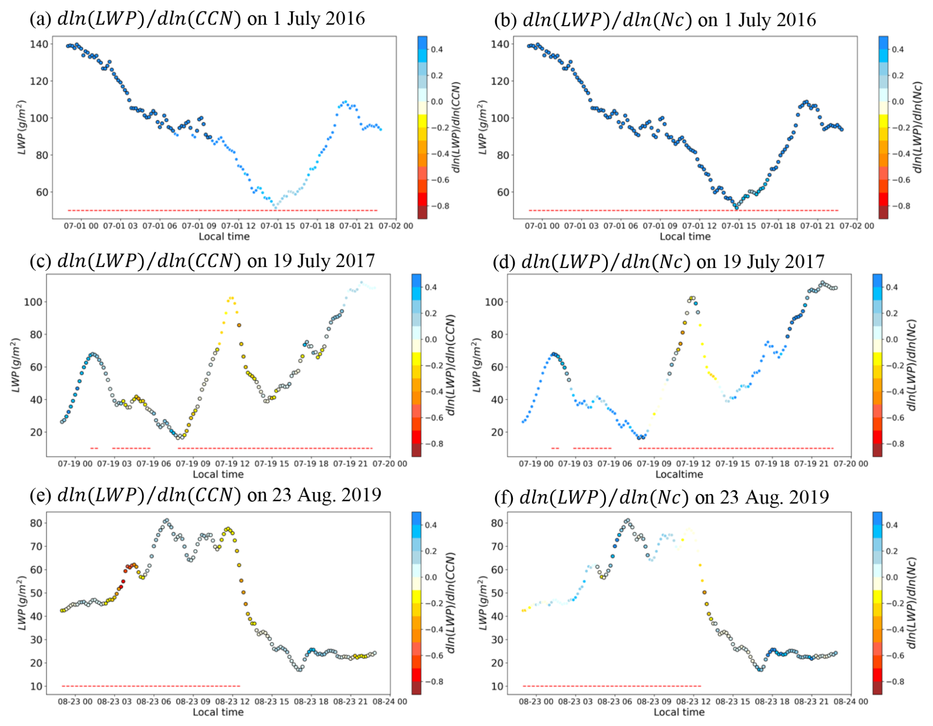
Figure 12 Panels (a), (c), and (e) are the temporal variability in the LWP susceptibility for different CCN concentrations, denoted as (dln (LWP)/dln (CCN)), on 1 July 2016, 19 July 2017, and 23 August 2019, respectively. Panels (b), (d), and (f) are the temporal variability in the LWP susceptibility for different N_c concentrations, denoted as (dln (LWP)/dln (N_c)), on 1 July 2016, 19 July 2017, and 23 August 2019, respectively. The logarithmic slope between the LWP and CCN is calculated at each output time (every 10 min) using data from 16 aggregate grid points (∼ 25 km for each grid point) from the control run and 16 aggregated grid points from the perturbed run. Black circles indicate statistically significant results with p ≤ 0.01. The dashed red lines indicate when the rainfall intensity is higher than 0.001 mm 10 min⁻¹ in domain 4.

To further illustrate the reduction in the LWP due to evaporation at the cloud edge, Fig. 13 presents the relative change in ln (LWP) between the perturbed and control cases across different LWP percentile ranges in the control case during the periods of negative LWP susceptibility, as shown in Fig. 12. The results indicate a decrease in the LWP in the perturbed cases compared to the control cases for pixels with the lowest LWP percentile range (0 %–25 %). We assume that this range corresponds to thin clouds at the edges of the cloud cover.

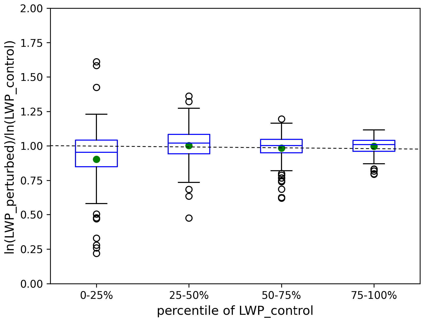
Figure 13 Box plot of the relative change in ln (LWP) between the perturbed and control cases across different LWP percentile ranges in the control case during the negative susceptibility for the LWP shown in Fig. 12. The box extends from the first quartile to the third quartile of the data, with a line at the median. The whiskers extend from the box to the farthest data point lying within 1.5× the interquartile range from the box. Outlier values are those past the end of the whiskers. Green dots are the mean value, and the dashed black line indicates the value of 1.0.

Figure 11b and d display the mean R_e susceptibilities for different CCN number and N_c values, respectively. The results consistently show that the radius of the cloud droplets decreases as CCN number or N_c increases. Additionally, the change in R_e is more pronounced when N_c (or CCN number) is higher.

In this study, the logarithmic slope between the LWP and CCN in the LWP susceptibility calculation is based on a linear assumption. Hoffmann et al. (2024) introduced a heuristic model that represents a significant advancement in understanding the process-level adjustments of cloud water in stratocumulus clouds, suggesting that the relationship may resemble a reversed “V” shape. Figure 13 indicates that the decrease in the LWP (negative susceptibilities) in the perturbed cases occurs only in low-LWP clouds (thin and non-rain clouds). Conversely, the LWP increases (positive susceptibilities) in thicker, precipitating clouds under the perturbed scenarios, which is consistent with the findings of Hoffmann et al. (2024). As our study aggregates grids to a 25 km resolution, we are able to capture such spatial heterogeneity and retrieve a negative susceptibility due to the evaporation of thin clouds at cloud edge, whereas at 100 km scale (domain average shown in Figs. S11 and S12), the signal is dominated by the increase in the LWP at cloud core. However, based on the current study cases, we may not have sufficient data samples to illustrate a relationship beyond the linear assumption.

4 Discussion and summary

This study focuses on aerosol indirect effects (AIEs), particularly involving the long-range transport of aerosols, in the eastern North Atlantic (ENA) region. It specifically examines these effects on warm boundary layer stratiform clouds located on the eastern side of oceanic subtropical highs under three different weather regimes: a ridge with a surface high-pressure system, a post-trough with a surface high-pressure system, and a weak trough. We select three specific case studies (i.e., 20160701, 20170719, and 20190823) to assess the impact of long-range-transported aerosols on warm boundary layer clouds, with each case representing a typical meteorological regime observed over the ENA site.

To investigate aerosol–cloud interactions more realistically, incorporating aerosol chemistry components that activate to cloud condensation nuclei (CCN) and accounting for aerosol spatiotemporal variation, this study employs the Weather Research and Forecasting model coupled with a chemistry component (WRF-Chem). This approach provides a detailed examination of AIEs in the ENA region under the three specified weather regimes. We employ a downscaling technique to conduct WRF-Chem simulations for the two inner domains (with the outer domains utilizing WRF). This approach results in nearly a 50 % reduction in total computational costs, achieving a throughput of 8 h d⁻¹ using 1080 cores.

We incorporate major aerosol species (BC, OC, and SO₄) and SO₂ from MERRA-2 to provide aerosol initial and boundary conditions, labeled as control cases. Additionally, we formulate three perturbed cases by amplifying aerosol concentrations in both the initial and boundary conditions and the sea salt emissions by a factor of 5 relative to each control case. As aerosol features are primarily determined by aerosol initial and boundary conditions, a higher Aitken-mode assumption in the major aerosol component (i.e., SO₄) regarding the aerosol mode ratio (80 % for the Aitken mode and 20 % for the accumulation mode) results in fewer aerosols activating as CCN due to the curvature effect in our simulations.

The WRF-Chem model captures the cloud structure in the case of 20160701 but underestimates the cloud amount. It simulates the formation of thin, uniform stratocumulus clouds within a meteorological regime characterized by a ridge system in the free troposphere and a high-pressure system near the surface. However, the cases of 20170719 and 20190823 exhibit the development of thicker but broken solid stratocumulus clouds within a post-trough regime and a weak trough, respectively. With the fast-moving cloud systems and strong surface wind, the WRF-Chem model struggles to capture the development and movement of these cloud systems due to delayed moisture transport from outer boundary condition and potential insufficient vertical resolution.

In all cases, compared to the observations, the WRF-Chem model underestimates the liquid water path (LWP) and cloud fraction due to a warmer and lower simulated boundary layer. In the perturbed cases, we find a 57 % higher aerosol-induced LWP, especially for the rain grids. We also note that the perturbed cases exhibit lower rainfall intensity, indicating a rainfall suppression effect attributed to high CCN concentrations, as concluded in previous studies (Wang et al., 2020; Christensen et al., 2024). In contrast, the LWP over the non-rain grids only increases by 28 %. Moreover, when introducing aerosols in the perturbed runs, the results over the rain grids exhibit larger cloud drops and a wider radius spectrum compared to the results over the non-rain grids. This suggests that the presence of aerosols has a more pronounced effect on cloud properties within the rain grids. The non-rain grids over the cloud edge can have lower LWP because smaller cloud droplets are easy to evaporate.

Our study further elucidates the intricate feedback mechanisms governing aerosol–cloud interactions and aerosol properties. In both the post-trough and weak-trough regimes, we observe a pronounced tendency for the cloud structure to develop more open-cell stratocumulus clouds. At the peripheries of these clouds, the perturbed cases demonstrate a significant increase in the presence of small cloud droplets. This heightened abundance of smaller droplets promotes evaporation, thereby leading to a marked reduction in the LWP.

As these clouds evaporate, the aerosols that are released return to the accumulation mode. This transition enhances their likelihood of reactivating as CCN. Consequently, this cycle underscores the dynamic interplay between aerosol properties and cloud formation, highlighting how changes in aerosol concentrations can influence cloud microphysics and, ultimately, precipitation processes.

Additionally, the susceptibility of the LWP to changes in CCN concentration is quantified using the logarithmic slope between the LWP and CCN. Our result shows that when the CCN concentration is low, the LWP is sensitive to variations in CCN number, with a higher CCN number concentration leading to a higher LWP. However, when the mean CCN concentration is relatively high, the LWP is not as sensitive to changes in CCN, and the LWP susceptibilities are small in magnitude, with both positive and negative values. Those negative values are caused by the evaporation from small cloud droplets in non-rain grids on the cloud edge.

In Wang et al. (2020), the liquid water content (LWC) susceptibility for a light-precipitation case on 18 July 2017 also shows positive values based on three sensitivity runs with CCN concentrations of 10, 100, and 1000 cm⁻³. The cloud properties in their study are averaged over all cloud points in the innermost domain. We adopt the same method as Wang et al. (2020) to estimate the LWP susceptibility using the domain mean values, defined as Δln (LWP_perturbed−LWP_control) $/$ Δln (CCN_perturbed−CCN_control). This approach predominantly yields positive values for the LWP susceptibility across the three study cases (see Figs. S11 and S12). This suggests that the 25 km resolution is able to capture such spatial heterogeneity and retrieve a negative susceptibility due to the evaporation of thin clouds at the cloud edge, whereas at 100 km scale (domain average), the signal is dominated by the increase in the LWP at the cloud core.

Conversely, the LWP susceptibilities associated with varying cloud droplet numbers reported in Qiu et al. (2024b) reveal significant negative values in LWP susceptibility in response to high cloud droplet numbers, a trend that is partially reflected in our study. Further investigation is required to reconcile the difference in the LWP responses between observational data and model simulations. Additionally, a more accurate estimation of the LWP susceptibility to changes in the CCN concentration is necessary.

Moreover, future research will focus on addressing the identified issues within the model, such as improving the representation of transported aerosol size distributions, resolving the overly fragmented stratocumulus cloud layers with sharp boundary layer inversions, and comparing the modeled cloud susceptibilities with observational data through simulations of ship tracks and local aerosol perturbations.