Assessing the ability to quantify the decrease in NO_x anthropogenic emissions in 2019 compared to 2005 using OMI and TROPOMI satellite observations

There are great expectations about the detection and the quantification of NO_x emissions using NO₂ tropospheric columns from satellite observations and inverse systems. This study assesses the potential of the OMI-QA4ECV and TROPOMI satellite observations to improve the knowledge of European NO_x emissions at the regional scale and to inform about the spatio-temporal variability of NO_x anthropogenic emissions in 2019 compared to 2005, at the resolution of 0.5° over Europe. We first characterize the level of consistency between retrievals from OMI-QA4ECV and from the more recent reprocessing of the TROPOMI data, called TROPOMI-RPRO-v02.04, and the implications of the possible inconsistencies for inversions. Furthermore, starting from European emission estimates from the TNO-GHGco-v3 inventory for the year 2005, regional inversions using the Community Inversion Framework coupled to the CHIMERE chemistry-transport model and assimilating satellite NO₂ tropospheric columns from OMI and TROPOMI have been performed to estimate the European annual and seasonal budgets for the year 2019. Both the OMI and TROPOMI inversions show decreases in European NO_x anthropogenic emission budgets in 2019 compared to 2005. Nevertheless, the magnitude of the reductions of the NO_x anthropogenic emissions is different with OMI and TROPOMI data, with decreases in EU-27 + UK between 2005 and 2019 of 16 % and 45 %, respectively. A TROPOMI inversion giving more weight to the satellite data becomes consistent with the independent TNO-GHGco-v3 inventory for the year 2019, with annual budgets for EU-27 + UK showing absolute relative difference of only 4 %. These TROPOMI inversions are therefore in agreement with the magnitude of the decline in NO_x emissions declared by countries, when aggregated at the European scale. However, our results – with OMI and TROPOMI data leading to different magnitudes of corrections on NO_x anthropogenic emissions – suggest that more observational constraints would be required to sharpen the European emission estimates.

1 Introduction

Air pollution is still a major health concern in Europe (EEA, 2023). Particularly, up to now all European Union (EU) countries have reported levels of nitrogen dioxide (NO₂) above the 2021 World Health Organization (WHO) global air quality guidelines, and around 64 000 premature deaths are caused by NO₂ pollution each year (EEA, 2023). In Europe, the main sources of NO₂ are road transport – responsible for 39 % of the emissions in 2019 (EEA, 2022), thermal power plants and industrial activities (EEA, 2023). NO₂ is mainly produced in the atmosphere by the oxidation of nitric oxide (NO), which is emitted by the same activities.

To reduce NO₂ concentrations to levels that do not impact human health, the emissions of nitrogen oxides (NO_x = NO + NO₂) need to be cut down. The EU has comprehensive regulations governing air quality. The key legal instrument in this regard is the Ambient Air Quality Directive (2008/50/EC). In addition, there are other EU regulations and directives that address specific aspects of air quality, such as the National Emission Ceilings (NEC) Directive (2016/2284/EU) (OJE, 2016), which sets expected reductions of NO_x emissions compared with 2005, often considered the baseline year of regulation policies. To design efficient regulatory policies and assess their effectiveness, an accurate account of emissions in space and time is essential.

Budgets and sectoral distributions for air pollutants often come from bottom-up (BU) inventories, based on the statistics of socio-economic activities and fuel consumption and on emission factors per activity type. According to these BU inventories, NO_x anthropogenic emissions have been strongly decreased – by about 36 % – in Europe since 2005 (EEA, 2021). However, the quantification of anthropogenic NO_x emissions following a BU approach suffers from relatively large uncertainties, especially from those in the emission factors, for which average values are generally used despite the large spatial and temporal variability of the actual factors. For instance, the European Monitoring and Evaluation Programme (EMEP) inventory reports 50 %–200 % uncertainties in their sectoral budgets of NO_x anthropogenic emissions at the national and annual scales (Kuenen and Dore, 2019). According to Schindlbacher et al. (2021), the uncertainty estimates for national anthropogenic NO_x emissions range from 5 % to 56 % in Europe. The spatial distribution and temporal variability of the time series of emission inventory maps often rely on simple proxies and typical temporal profiles, which inevitably introduce errors. Quantifying natural (biogenic) emissions is also a complex issue (Guenther et al., 2006).

Since the year 2000, observations of the atmospheric concentrations of nitrogen dioxide (NO₂) have been retrieved from space-borne spectrometers with suitable measurement spectral bands, such as the Global Ozone Monitoring Experiment (GOME) (Burrows et al., 1999), GOME-2 (Munro et al., 2016), the SCanning Imaging Absorption spectroMeter for Atmospheric CHartographY (SCIAMACHY) (Burrows et al., 1995; Bovensmann et al., 1999) and the Ozone Monitoring Instrument (OMI) (Levelt et al., 2006, 2018). These instruments offer a daily global coverage with horizontal resolutions of several hundreds of kilometers squared. The satellite observations provide information on the chemical composition of the atmosphere and for the analysis of the variations of the NO₂ concentrations associated with economic changes or pollution control legislation over the last decades (van der A et al., 2008; Castellanos and Boersma, 2012; Schneider et al., 2015; Lamsal et al., 2015; Krotkov et al., 2016; Miyazaki et al., 2017; Li and Wang, 2019; Georgoulias et al., 2019; Silvern et al., 2019; Fortems-Cheiney et al., 2021a; van der A et al., 2024).

In parallel, progress has been made to develop atmospheric transport and chemistry inverse modeling for the estimation of NO_x anthropogenic and/or biogenic emissions based on the satellite observations of the NO₂ tropospheric vertical column densities (TVCDs), also referred to as top-down (TD) or inverse modeling. Such systems generally rely on the comparison between observed TVCDs and NO₂ simulations based on atmospheric chemistry transport models and on emission estimates from BU gridded inventories and land-surface models, to retrieve optimal emission estimates. The retrieval of these emission estimates assumes the discrepancies between simulated and observed TVCDs to be mainly due to these BU emission estimates.

However, the discrepancies between simulated and observed TVCDs are also due to errors in the modeling of the atmospheric transport and chemistry of NO_x (Stavrakou et al., 2013) and in the observations due to instrumental errors and retrieval biases (Lorente et al., 2017). The retrieval of TVCDs with the corresponding averaging kernels relies on the local inverse modeling of the radiative transfer in the atmosphere under various and often complex atmospheric and surface conditions, which is challenging (Boersma et al., 2004; van Geffen et al., 2022a). Therefore, the intercomparisons of the different NO₂ retrieval products based on measurements from a specific satellite instrument but different algorithms reveal large differences. For instance, the magnitude of the OMI NO₂ TVCDs of OMI-NASAv3 (from the National Aeronautics and Space Administration; NASA) and of OMI-DOMINOv2 (from the Royal Netherlands Meteorological Institute; KNMI) differs by 50 % over densely populated areas in China, and they show different trends over the past decade at the regional scale (Zheng et al., 2014; Qu et al., 2017; Lorente et al., 2017). Qu et al. (2020) compared OMI-NASAv3, OMI-DOMINOv2 and the Quality Assurance for Essential Climate Variables (OMI-QA4ECV) OMI NO₂ TVCD product and showed that the different vertical sensitivities in the NO₂ retrievals explain most of the discrepancies between the retrieved NO₂ TVCDs.

The first NO_x atmospheric inversions using satellite NO₂ data were generally based on global systems and targeted the variability of the NO_x emissions at continental scales (Martin et al., 2003; Boersma et al., 2008; Stavrakou et al., 2008; Lamsal et al., 2011; Miyazaki et al., 2017). The scientific and societal needs for the quantification and mapping of pollutant emissions at a relatively high-spatial resolution fostered the use of regional-scale inversion systems, based on mesoscale chemistry-transport models (CTMs) and the analysis of the NO₂ concentrations at spatial resolution close to that of the satellite observations (Mijling and van der A, 2012; Mijling et al., 2013; Lin, 2012; Ding et al., 2017; Visser et al., 2019; Fortems-Cheiney et al., 2021b; Savas et al., 2023; van der A et al., 2024) and even down to a resolution of 10 km × 10 km (Plauchu et al., 2024).

The computation cost of the regional atmospheric inversions can be potentially high, due to the need to rely on high-spatial-resolution CTMs and to manage high-dimension inversion problems for the estimation of NO_x emissions at relatively fine spatio-temporal scales that support the derivation of robust monthly to annual and national to sub-national budgets. To mitigate this computational cost, mass balance approaches have been employed (Visser et al., 2019). These approaches account for the non-linear relationships between NO_x emission changes and NO₂ TVCDs via reactions with hydroxyl radicals (OH) but with simple scaling factors. Stavrakou et al. (2013), Ding et al. (2017) and van der A et al. (2024) tend to indicate that a more robust account for the complex NO_x chemistry is required for the accurate derivation of NO_x emissions from NO₂ satellite data. In addition, with such an approach the emissions are scaled so that the CTM simulations fit the observations perfectly; therefore the errors from both the CTM and the retrievals are ignored, which can limit the accuracy of the inversions (Miyazaki et al., 2017). In this context, the complex Bayesian approaches with ensemble Kalman filter or variational inverse modeling techniques relying on CTMs may have a key role to play, since they are designed to take into account both (i) the non-linearities of the NO_x chemistry and (ii) the errors from the CTMs and retrievals.

Since 2017, the TROPOspheric Monitoring Instrument (TROPOMI; Veefkind et al., 2012) on board the Copernicus Sentinel-5 Precursor (S5P) has been providing NO₂ TVCDs images (over a wide swath) at higher spatial resolutions and improved signal-to-noise ratio, compared to previous missions such as OMI (van Geffen et al., 2020). With variational inversions, Plauchu et al. (2024) assessed the potential of the TROPOMI observations to inform about NO_x emissions in France from 2019 to 2021 at national to urban scales. Their results open positive perspectives regarding the ability of inversions to support the validation or improvement of inventories with TROPOMI observations, at least at the local level for emission hotspots generating a relatively strong local signal, which are better caught and exploited by the inversions than the larger-scale signals (Plauchu et al., 2024). While previous satellite instruments could already provide information over emission hotspots (e.g, over large urban areas in Europe; Fortems-Cheiney et al., 2021a), TROPOMI might now be more relevant than these previous satellite instruments to monitor the NO_x anthropogenic emissions (Zheng et al., 2020; Li et al., 2023).

In this context, this study assesses the respective potential of the OMI and TROPOMI satellite observations to inform about the decrease in NO_x anthropogenic emissions in 2019 compared to 2005 at the continental to national scales in Europe, based on a state-of-the-art regional variational inverse modeling system. The concept is to assess the level of decrease in the emission estimates for the year 2019 from the atmospheric inversions assimilating OMI or TROPOMI observations for this year, compared to the prior estimate that they correct to better fit the observations and which corresponds to an inventory for the year 2005. Such a concept accounts for the absence of TROPOMI observations in 2005, but parallel tests (e.g., with OMI observations in 2005) are conducted to ensure that this decrease fairly reflects the level of decrease in emissions between 2005 and 2019 caught by the inversions.

In practice, we have performed 1-year inversions using an estimate of the NO_x anthropogenic emissions from the TNO-GHGco-v3 inventory (Dellaert et al., 2021) for the reference year 2005 to define the prior estimate of the variational inversions. The evaluation of the emissions estimated from the inversions is based on comparisons to the NO_x emission estimates from the TNO-GHGco-v3 inventory for the year 2019. We use a European-scale variational inverse modeling system at 0.5° and 1 d resolution based on the coupling of the variational mode of the Community Inversion Framework (CIF) (Berchet et al., 2021) to a 0.5° resolution configuration of the regional CTM CHIMERE (Menut et al., 2013). Our inversion system combines the advantages of both (i) solving large dimensional inversion problems, i.e., controlling emissions at relatively high temporal and spatial resolution and assimilating a large amount of observations, and (ii) simulating NO₂ concentrations and the sensitivities of NO₂ tropospheric columns to surface emissions at a relatively high spatial resolution with a chemistry scheme, based on CHIMERE and its adjoint code. Our inversion system is therefore well designed to estimate NO_x emissions at the 0.5° and 1 d resolutions, taking into account the non-linearities of the NO_x chemistry. The CIF-CHIMERE variational inversion configuration has already been used for the estimation of the emissions of NO_x (Savas et al., 2023; Plauchu et al., 2024) but also of other species such as CO (Fortems-Cheiney et al., 2024) and CO₂ (Petrescu et al., 2023).

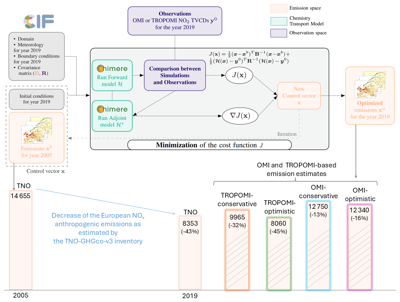
Figure 1 Simplified scheme of the iterative minimization in the CIF-CHIMERE inversion system and illustration of the decrease in the European NO_x emissions estimated both by TNO and by the OMI and TROPOMI-based inversions. The different inversions are described in Table 1. The numbers express the anthropogenic NO_x emission estimates for the EU-27 + UK area (in kteq NO₂). The numbers in brackets express the difference of the anthropogenic NO_x emission estimates for the EU-27 + UK in 2019 compared to 2005 (in %).

As a preliminary analysis, we have also characterized the level of consistency between retrievals from OMI-QA4ECV and from the more recent reprocessing of the TROPOMI data, called TROPOMI-RPRO-v02.04, and the implication of the possible inconsistencies for inversions. The regional 0.5° resolution simulations of NO₂ TVCDs in Europe with CHIMERE are used to indirectly analyze this consistency via the respective differences between the two NO₂ TVCD products and CHIMERE. In the following, we first describe the CHIMERE configuration for Europe, the NO₂ satellite observations and the variational inversion method in Sect. 2. Section 3 presents our results, including the comparison between the CHIMERE simulations, the OMI and TROPOMI NO₂ TVCDs, and the posterior estimates of NO_x European anthropogenic emissions.

Table 1 Description of the inversions performed in this study.

2 Data and methods

The principle of our traditional atmospheric inversion approach is to correct a priori estimates of the emission maps, also denoted “prior emissions”, to reduce differences between atmospheric observations and their simulations with a CTM fed with the estimates of emission maps. It relies on a specific Bayesian inversion algorithm, on satellite observations of the atmospheric densities of NO₂, and on a regional CTM, as shown in Fig. 1. We detail these different components of our inversion framework: the CIF-CHIMERE variational inversion system, the prior estimates of the NO_x emissions in Europe for the year 2005, the configuration of the CHIMERE CTM and of its adjoint code for the simulation of NO₂ concentrations and of their sensitivity to the emissions estimates, and the OMI-QA4ECV and TROPOMI satellite observations for the year 2019. The process ensuring suitable comparisons between the simulations and the satellite observations – the aggregation of the observations into super-observations and the application of the averaging kernels from the satellite retrievals to the vertical columns of the model simulations – is also explained. Finally, we provide details about our configuration for the inversion of NO_x emissions over Europe.

2.1 The CIF-CHIMERE inversion system

The Community Inversion Framework (CIF) is a modular inverse modeling platform which can drive various data assimilation schemes and various CTMs (Berchet et al., 2021). Here, the CIF drives the CHIMERE CTM (Menut et al., 2013; Mailler et al., 2017) and its adjoint code (Fortems-Cheiney et al., 2021b). The coupling between the CIF and CHIMERE and its adjoint code and their use for variational inversions takes advantage of the developments in the Bayesian variational atmospheric inversion system PYVAR-CHIMERE to account for reactive species (Fortems-Cheiney et al., 2021b).

2.2 Prior estimates of the NO_x emissions in Europe

The prior estimates of NO_x emissions in this study are based on anthropogenic NO_x emission estimates from the TNO-GHGco-v3 gridded inventory (Dellaert et al., 2021) for the year 2005. We have chosen such an estimate for year 2005 to assess the potential of satellite observations for year 2019 to quantify the high spatio-temporal differences in the NO_x emissions between 2005 and 2019. The NO_x emission estimates from the TNO-GHGco-v3 inventory for the year 2019 are used to evaluate the inversion results. We have also performed inversions (i) both using NO_x prior emissions and assimilating satellite observations for the year 2005 and (ii) both using NO_x prior emissions and assimilating satellite observations for the year 2019 (Table 1) to assess the impact of the prior inventory on the NO_x emissions estimated from the inversions.

The TNO-GHGco version is an update of the TNO inventory documented in Kuenen et al. (2014) and in Super et al. (2020), based on country emission reporting to the European Monitoring and Evaluation Program (EMEP)/Center on Emission Inventories Projection (CEIP). The TNO-GHGco-v3 inventory maps NO_x emissions at a 6 km × 6 km horizontal resolution. It combines emissions from area sources, set at the surface, and from point sources. Emissions from point sources, mainly from the energy production and the industrial sectors, are distributed on the first eight vertical model layers in CHIMERE depending on the typical injection heights provided in the TNO inventory, based on Bieser et al. (2011).

In the TNO inventory, annual and national budgets are disaggregated in space based on proxies of the different sectors (Kuenen et al., 2014). Temporal disaggregation is based on temporal profiles provided per GNFR sector code with typical month to month, weekday to weekend and diurnal variations (Ebel et al., 1994, Menut et al., 2011). Following the GENEMIS recommendations (Kurtenbach et al., 2001; Aumont et al., 2003), we have speciated the TNO-GHGco-v3 NO_x emissions as 90 % of NO, 9.2 % of NO₂ and 0.8 % of nitrous acid (HONO) emissions.

CHIMERE is fed with NO biogenic soil emissions from the Model of Emissions of Gases and Aerosols from Nature (MEGAN) for the year 2019 (Guenther et al., 2006), with a ∼ 1 km × 1 km spatial resolution. MEGAN does not take the impact of agricultural practices into account, even though it covers both natural and agricultural areas. There are large uncertainties in the NO_x emissions due to agriculture, and in principle, there could be some overlapping between the agricultural and purely natural soil NO_x emission estimates. It explains why these emissions are not provided by the TNO inventory. Therefore, we do not include a specific agricultural soil NO_x emissions component in our prior estimation of the NO_x emissions. The lightning NO_x fluxes, whose impact on NO₂ concentrations is very small in Europe even in summer (Menut et al., 2020), are not accounted for. Fire emissions are also ignored, as their contribution to the NO_x total emissions and to the long-term NO₂ concentration trends over Europe is small. The anthropogenic emissions for volatile organic compounds (VOCs) are obtained from the EMEP inventory (Vestreng et al., 2005).

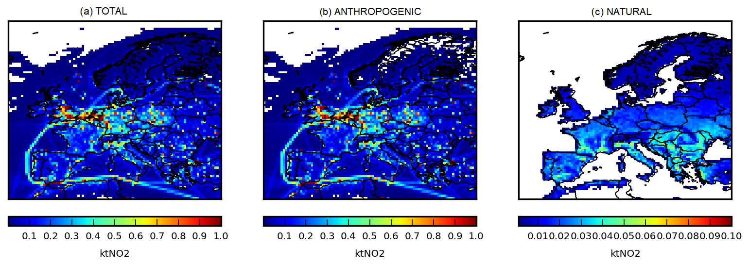
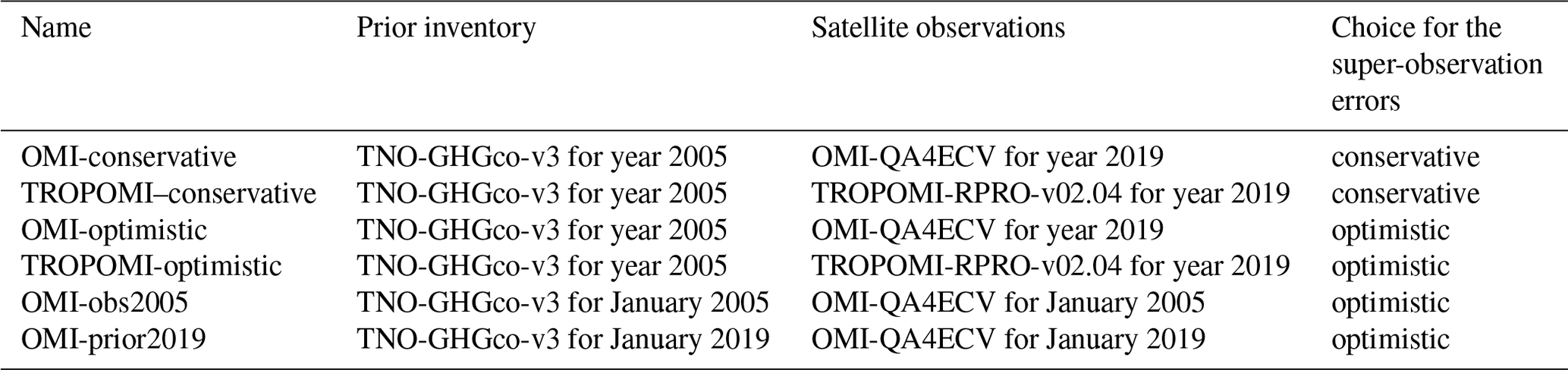
Figure 2 Monthly budget of prior NO_x emissions corresponding to the (a) total, (b) anthropogenic from the TNO-GHGco-v3 inventory and (c) biogenic from the MEGAN model, per model grid cell (in kteq NO₂) in August 2019. Note that the scale is different for anthropogenic and biogenic emissions.

The different emission products have been aggregated at the 0.5° × 0.5° horizontal resolution of the CHIMERE grid. The maps of monthly budgets for total, anthropogenic and natural NO_x emissions at 0.5° resolution are shown in Fig. 2 for August 2019. Even in summer when the biogenic NO_x emissions are high, the anthropogenic emissions contribute to about 95 % of the total NO_x emissions in Europe with a budget of about 815 kteq NO₂. This unit means that the mass of both NO and NO₂ emissions is calculated using the NO₂ molar mass.

2.3 Configuration of the CHIMERE CTM for the prior simulation of NO₂ concentrations in Europe

We present the configuration of the CHIMERE CTM used in this study and the specific elements of the simulation, which will be used as the prior of the variational inversions. Here, the configurations of CHIMERE and of its adjoint code are driven by the CIF to simulate NO₂ atmospheric concentrations over Europe over a 0.5° × 0.5° regular horizontal grid with 17 vertical layers, from the surface to 200 hPa, with 8 layers within the first 2 km. The domain covers 31.75–74.25°N, 15.25° W–35.75° E and includes 101 (longitude) × 85 (latitude) × 17 (vertical levels) grid cells.

The chemical scheme used here is MELCHIOR-2, with more than 100 reactions, including 24 for inorganic chemistry (Lattuati, 1997; Derognat et al., 2003). It accounts for non-linear relationships between NO_x emission changes and NO₂ TVCDs via reactions with hydroxyl (OH) radicals but also with other direct or indirect NO_x sinks associated with other species, such as ozone (O₃) or the HO₂ radical. Due to the need for a compromise between the robustness of the simulation of the chemistry in the model and the computational cost with a complex chemical scheme, the aerosol modules of CHIMERE have not been included in its adjoint code yet and are therefore not activated in the CHIMERE forward simulations, as explained in Fortems-Cheiney et al. (2021b).

CHIMERE is driven here by the European Centre for Medium-Range Weather Forecasts (ECMWF) operational meteorological forecast for the year 2019 (Owens and Hewson, 2018). Considering the short lifetime of NO₂, we do not consider its import from outside the domain. Nevertheless, the lateral and top boundaries for longer lived species such as ozone (O₃), nitric acid (HNO₃) and peroxyacetyl nitrate (PAN), which participate in the NO_x chemistry, are taken into account (Fortems-Cheiney et al., 2021b). Climatological values from the LMDZ-INCA global model (Szopa et al., 2008) are used to prescribe the concentrations of these species at the model boundaries.

2.4 Satellite observations

Among the instruments providing a long archive of NO₂ observations, OMI has the highest spatial resolution and least degradation through time (Levelt et al., 2018; Schenkeveld et al., 2017). OMI and TROPOMI present similarities: the retrievals from TROPOMI and from OMI-Q4ECV are based on similar algorithms, using the same prior profiles and assimilation technique to estimate the stratospheric column from the global model TM5-MP, and they make measurements at nadir at about the same local time. Therefore, we expect these datasets to be consistent, with similar NO₂ TVCDs over horizontal and temporal scales larger than a few hundred kilometers resolution and the month. Nevertheless, a comparison of TROPOMI version 01.03 NO₂ TVCDs to OMI-QA4ECV observations shows differences in terms of monthly NO₂ average varying from a few percent up to −40 % over polluted regions (western Europe, eastern China, eastern USA, the Middle East), the largest differences occurring in winter (Lambert et al., 2021). Comparisons with ground-based measurements have also shown that versions v01.02 and v01.03 of TROPOMI data lead to NO₂ TVCDs that are too low by 22 % to 37 % for clean and slightly polluted scenes, and up to 51 % over highly polluted areas (Verhoelst et al., 2021). Efforts have been made to correct such biases in the recent versions of the TROPOMI data and seem to lead to better agreement with OMI-QA4ECV observations and with ground-based measurements (Lambert et al., 2021; van Geffen et al., 2022b, a).

As significant biases between the OMI and TROPOMI tropospheric columns have been described in previous studies in winter (Lambert et al., 2021; Verhoelst et al., 2021; van Geffen et al., 2022b), the month of January 2019 is being particularly used to compare these observations in the following.

2.4.1 OMI-QA4ECV-v1.1

The Ozone Monitoring Instrument (OMI) is an ultraviolet-visible (UV-Vis) instrument launched in July 2004 on board the Earth Observation System (EOS) Aura satellite, which flies on a 705 km sun-synchronous orbit that crosses the Equator at approximately 13:40 LT. The nominal footprint of the OMI ground pixels is 24 km × 13 km (across × along track) at nadir. With a swath of about 2600 km, it provided daily global coverage for NO₂ (no longer achieved due to the row anomaly). OMI uses the O₂–O₂ absorption feature for the cloud pressure retrieval (Veefkind et al., 2016).

The NO_x inversions described in Sect. 2.5 assimilate NO₂ TVCDs from the OMI-QA4ECV-v1.1 (http://www.qa4ecv.eu, last access: September 2023, and http://temis.nl/qa4ecv/no2.html, last access: September 2023, Boersma et al., 2017, 2018). The data selection follows the criteria of the data quality statement (Boersma et al., 2017): the processing error flag equals 0, the solar zenith angle is lower than 80°, the snow ice flag is lower than 10 or equal to 255, the ratio of tropospheric air mass factor (AMF) over geometric AMF is higher than 0.2 to avoid situations in which the retrieval is based on very low (relative) tropospheric air mass factors, and the cloud fraction is lower than 0.5. We use an additional criterion for the selection of the observation to be assimilated: the error associated with the retrieval must be lower than 100 %. Note that the OMI-QA4ECV-v1.1 reprocessed datasets officially covers the period 2005–2018. This processing uses ERA-Interim 60-layer meteorological reanalyses from the ECMWF as the driver. To facilitate comparisons with TROPOMI, the OMI dataset was further extended to 2019 using 137-layer ECMWF operational meteorological data. For 2019, the pressure levels are identical for the OMI and TROPOMI products.

2.4.2 TROPOMI RPRO-v02.04

The Tropospheric Monitoring Instrument (TROPOMI; Veefkind et al., 2012) was launched on board the Copernicus Sentinel-5 Precursor (S5P) satellite in October 2017. It flies on a 824 km altitude sun-synchronous orbit that crosses the Equator at approximately 13:40 LT. This imaging spectrometer covers a UV–Vis band supporting the derivation of NO₂ TVCDs observations. The nominal footprint of the TROPOMI ground pixels is of about 7 km × 3.5 km before 6 August 2019 and 5.5 km × 3.5 km after 6 August 2019 at nadir. With a swath of about 2600 km on ground, it provides daily global coverage for NO₂. Actually, one of the differences between the OMI and TROPOMI retrievals is the cloud pressure retrieval, which could have large impacts on the results. In particular, the Fast Retrieval Scheme for Clouds from Oxygen absorption band FRESCO-S version implemented for TROPOMI in v01.00 to v01.03 has been known to overestimate the cloud pressure, leading to a high bias in the air mass factors and a low bias in the tropospheric columns (Lambert et al., 2021). In addition, TROPOMI-v02.04 uses the TROPOMI dependent Lambertian-equivalent reflectivity (DLER) v1.0 surface albedo dataset (Tilstra et al., 2024), in contrast to OMI which makes use of the OMI Lambertian equivalent reflectance (LER) (Kleipool et al., 2008). Furthermore, TROPOMI applies dynamic albedo adjustments (van Geffen et al., 2022a), which is not done in the OMI-QA4ECV dataset.

Our selection of the TROPOMI data to be assimilated in the inversions described in Sect. 2.5 follows the criteria of van Geffen et al. (2022b). We only select observations with a quality assurance (qa) value higher than 0.75. Like OMI, we only select observations when the error associated with the retrieval is lower than 100 %.

Figure 3 Median and quartile profiles of averaging kernels from OMI-QA4ECV and TROPOMI-RPRO-v02.04 super-observations over continental land, for NO₂ TVCDs lower and higher than 2 × 10¹⁵ $\mathrm{molec}.{\mathrm{cm}}^{-\mathrm{2}}$, for the first six levels of the satellites, in January 2019.

2.4.3 Choices made to ensure a consistent comparison between simulated and observed NO₂ TVCDs

OMI and TROPOMI have different horizontal resolutions and more generally a different spatio-temporal sampling. The comparison between the data from the two instruments, as well as the comparisons to the simulated TVCDs, has therefore been done over a common projection, within the 0.5° × 0.5° grid cells of the CHIMERE CTM.

To make comparisons between simulations and satellite observations, the simulated vertical profiles are first interpolated on the satellite's levels, with a vertical interpolation from CHIMERE's levels. Then, the averaging kernels (AKs) from the OMI and TROPOMI products, respectively, are applied to the simulated profiles to account for the variations of the vertical sensitivity of the satellite retrievals (Eskes and Boersma, 2003; Boersma et al., 2017; van Geffen et al., 2022b). It is important to note that the OMI and the TROPOMI observations are accompanied with differences in their AKs, mainly explained by differences in their cloud pressure retrievals. The lower spatial resolution of OMI compared to TROPOMI also leads to differences in the distribution of the effective cloud fractions, with TROPOMI having relatively more cloud-free and fully clouded pixels, which impacts the AKs and their shapes. Over land, OMI and TROPOMI present similar sensitivity near the surface, both over polluted areas defined as areas where the NO₂ TVCDs are higher than 2 × 10¹⁵ $\mathrm{molec}.{\mathrm{cm}}^{-\mathrm{2}}$ and over rural areas (Fig. 3). However, due to lower cloud pressures on average in OMI than TROPOMI and consequently smaller air mass factors (AMFs) in the middle to lower troposphere, the AKs in OMI tend to be smaller than in TROPOMI above the first four levels of the satellites. These different vertical sensitivities and amplitudes of the AKs in the NO₂ OMI and TROPOMI retrievals will affect the simulated NO₂ TVCDs over Europe.

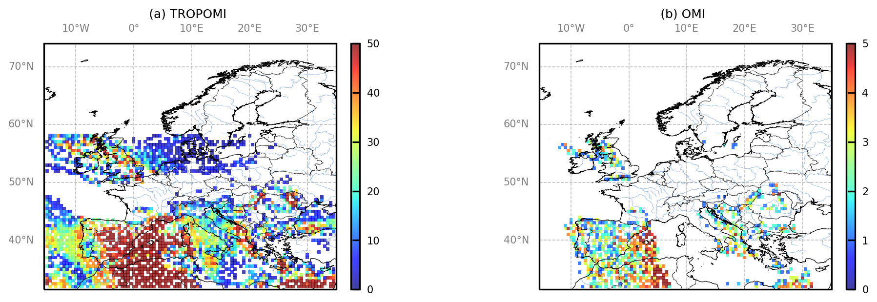
Figure 4 Daily number of observations within (a) TROPOMI and (b) OMI super-observations, for 1 January 2019. Note that the scales are different for TROPOMI and OMI.

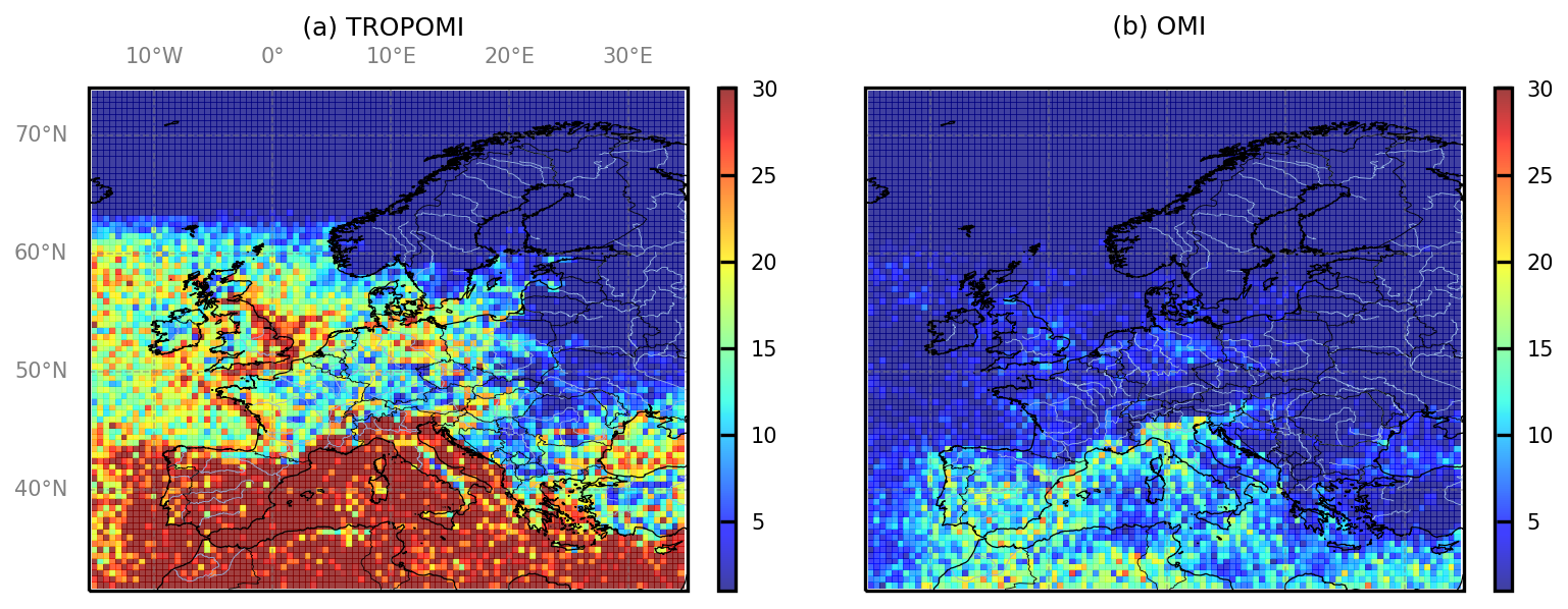
Figure 5 Monthly number of (a) TROPOMI and (b) OMI super-observations, in January 2019.

As the spatial resolution of OMI or TROPOMI data is finer than that of the chosen CTM model grid, the selected OMI or TROPOMI TVCDs are aggregated into “super-observations”, as recommended by Rijsdijk et al. (2025). In order to associate the super-observations to an actual AK profile, the super-observations have been taken as the observation (TVCD and AKs) corresponding to the value closest to the mean of the OMI or TROPOMI TVCDs within the 0.5° × 0.5° model grid cell and within the CHIMERE physical time step of about 5–10 min, as in Plauchu et al. (2024). The choice of the value closest to the mean is different from Fortems-Cheiney et al. (2021b), initially taking the median of the observations for defining super-observations. This choice was made necessary by the high number of TROPOMI observations within the 0.5° × 0.5° model grid cell. The number of TROPOMI observations within a TROPOMI super-observation can reach 50, while the number of OMI observations within an OMI super-observation is often lower than five over continental land (Fig. 4). We assume that over a set of a few tens of data the mean of the observations is more representative than the median, particularly in grid cells with high concentrations. The number of TROPOMI and OMI super-observations is given as an example for the month of January 2019, respectively, in Fig. 5a and in Fig. 5b. The TROPOMI super-observations present a coverage higher than the OMI ones by about a factor 4 (about 117 000 against 27 000). The only areas not really covered by TROPOMI are north-eastern Europe because of the snow cover and northern Europe because of the high solar zenith angle (Fig. 5a).

The simulated NO₂ TVCDs corresponding to the OMI super-observations, using the OMI AKs, are called “CHIMERE-OMI”. Similarly, the simulated NO₂ TVCDs corresponding to the TROPOMI super-observations, using the TROPOMI AKs, are called “CHIMERE-TROPOMI” in the following.

Various choices can be made for the derivation of the error associated with each super-observation. First, the error associated with each super-observation can be derived from the observation closest to the mean value, as in Plauchu et al. (2024). In this case, the derivation of the error associated with each super-observation, referred to as “OMI-conservative” or “TROPOMI-conservative” in the following, is conservative compared to other studies, where the super-observation uncertainty is reduced compared to that of individual observations (Boersma et al., 2016). The reduction of uncertainty when combining several observations accounts for the fact that the retrieval errors include random noise (in particular, instrumental noise without spatial correlation, i.e., errors which are independent from one observation to the other). However, OMI or TROPOMI NO₂ observations probably bear systematic errors from the instrument and from the retrieval process, which can exhibit important spatial correlations (Rijsdijk et al., 2025). This can justify a conservative attribution of observation errors to the super-observations.

Nevertheless, in addition to this configuration, we have also performed a sensitivity test, referred to as “OMI-optimistic” or “TROPOMI-optimistic” in the following (Table 1), where the error associated with each super-observation is derived as the error from the observation closest to the mean value multiplied by a factor of $\frac{\mathrm{1}}{\sqrt{\text{nbobs}}}$, where nbobs is the number of observations within a super-observation. In this case, the corresponding super-observation error is smaller than that of the individual observations.

2.5 Variational inversion of the NO_x emissions

The principle of our atmospheric inversions is to correct prior emission maps from the TNO-GHGco-v3 gridded inventory for the year 2005 (presented in Sect. 2.2) and initial conditions, by reducing differences between CHIMERE simulations and OMI-QA4ECV or TROPOMI-RPRO-v02.04 satellite data for the year 2019 as shown in Fig. 1, using a variational inversion framework similar to that of Plauchu et al. (2024). Our new emission estimates are called “posterior” in the following. Over the entire year 2019, 1-month inversion windows – independent from each other – have been performed. For each inversion window, the posterior estimate of the emissions is found by iteratively minimizing the cost function J(x):

$$\begin{array}{rl}J\left(\mathit{x}\right)=& {\displaystyle \frac{\mathrm{1}}{\mathrm{2}}}(\mathit{x}-{\mathit{x}}^{\mathrm{b}}{)}^{\mathrm{T}}{\mathbf{B}}^{-\mathrm{1}}(\mathit{x}-{\mathit{x}}^{\mathrm{b}})\\ & +{\displaystyle \frac{\mathrm{1}}{\mathrm{2}}}\left(\mathcal{H}\right(\mathit{x})-\mathit{y}{)}^{\mathrm{T}}{\mathbf{R}}^{-\mathrm{1}}(\mathcal{H}\left(\mathit{x}\right)-\mathit{y}),\end{array}$$

where x, ℋ, y, B and R are, respectively, the control vector, the observation operator, the satellite observations, the prior error covariance matrix and the observation error covariance matrix. As in Plauchu et al. (2024), the definition of x ensures that the inversion solves separately for the two main types of NO emissions: the anthropogenic and the biogenic emissions (without any further sectorization or decomposition into more detailed emission components) and for the anthropogenic NO₂ emissions. With such a control vector, the prior NO / NO₂ anthropogenic emission ratio speciation from the GENEMIS recommendations (see Sect. 2.2) is not kept by the inversion. The analysis in the following focuses on the NO_x emissions as the sum of the NO and NO₂ emissions.

Contrarily to Fortems-Cheiney et al. (2021b), and as in Plauchu et al. (2024), the prior uncertainty in both the anthropogenic and biogenic NO_x emissions is characterized with log-normal distributions, allowing the inversion system to apply high variations in NO_x emissions while ensuring that the inversion keeps the emissions positive, unlike the classic corrections of the emissions with scaling factors. Details about this feature are given in Plauchu et al. (2024).

Our control vector x contains the following:

• the logarithms of the scaling coefficients for NO anthropogenic emissions at a 1 d temporal resolution, at a 0.5° × 0.5° (longitude, latitude) horizontal resolution and over the first eight vertical levels of CHIMERE i.e, for each of the corresponding 101 × 85 × 8 grid cells;

• the logarithms of the scaling coefficients for NO₂ anthropogenic emissions at the same temporal and spatial resolutions as for NO;

• the logarithms of the scaling coefficients for NO biogenic emissions at a 1 d temporal resolution, at a 0.5° × 0.5° (longitude, latitude) resolution and at the surface (over 1 vertical level only), i.e., for each of the corresponding 101 × 85 × 1 grid cells;

• factors scaling the NO and NO₂ 3D initial conditions at 00:00 UTC the first day of each month, at a 0.5° × 0.5° (longitude, latitude) resolution and over the 17 vertical levels of CHIMERE.

The uncertainties in the observations y together with those in the observation operator ℋ, and the uncertainties in the prior estimate of the control vector x, are assumed to have a Gaussian distribution. Here, the first block of B corresponds to the logarithms of the anthropogenic flux factors. Each diagonal element is set at (0.5)²: this variance value in the log-space corresponds to a factor ranging between 60 %–164 % in the emission space at the 1 d and model's grid scale. A second block is set for biogenic fluxes. On the diagonal, uncertainties are also set to a value of (0.5)², also corresponding to a factor ranging between 60 %–164 % in the emission space at the 1 d and model's grid scale. We account for spatial correlations in the uncertainties both for the anthropogenic and the natural parts. Spatial correlations are described by exponentially decaying functions with an e-folding length of 50 km over land and over the sea. Finally, in the third block of B for initial conditions, the variances are set at 20 %.

The variance of the observation errors corresponding to individual super-observations in R is the quadratic sum of the error we have assigned to the OMI or TROPOMI super-observations and of an estimate of the errors from the observation operator. We assume that the observation operator error is dominated by the chemistry-transport modeling error: it is set at 20 % of the retrieval value, as in Fortems-Cheiney et al. (2021b). The monthly averages of the observation errors in R are shown in Fig. 6 for the different configurations associated with the errors assigned to the OMI or TROPOMI super-observations (see Sect. 2.4.3). It is interesting to note that the TROPOMI-conservative configuration, ignoring the number of observations to reduce the error associated with the super-observation, presents lower errors than the OMI-conservative one. This is explained by the better signal-to-noise ratio of TROPOMI compared to OMI (van Geffen et al., 2022b).

The different experiments performed in this study are presented in Table 1. The inversions are conducted using the variational mode of the CIF with the limited-memory quasi-Newton minimization algorithm M1QN3 (Gilbert and Lemaréchal, 1989) for the minimization of the cost function J. At each iteration of this minimization, the CIF uses a CHIMERE simulation to compute J for a new estimate of x and the adjoint code of CHIMERE to compute the gradient of J for this new estimate of x. We impose a reduction of the norm of the gradient of J by 90 % as a constraint for the interruption of the minimization process, but the reduction of the norm of the gradient of J actually often exceeds 95 %.

3 Results

3.1 Comparison between OMI and TROPOMI super-observations

The NO₂ TVCDS from OMI-QA4ECV and older versions of the TROPOMI products have been compared in the literature. Sekiya et al. (2022) reported lower concentrations in TROPOMI unofficial reprocessing product (version 1.2 beta) than in OMI-QA4ECV by 15 % during April–May 2018 averaged over 60° S–60° N. As mentioned in the Introduction, Lambert et al. (2021) reported NO₂ TVCDs from TROPOMI version 01.02 and 01.03 products systematically lower than from OMI-QA4ECV, with differences in terms of monthly NO₂ average reaching −40 % over polluted regions in winter. Nevertheless, comparisons of TROPOMI-v01.04 with OMI-QA4ECV observations show an improved consistency between the two retrievals. Over Europe, while the bias was of about −17 % in January 2019 with version 01.03, it was of about −4 % in January 2020 with version 01.04 (Lambert et al., 2021). Here, we would like to characterize the consistencies between OMI-QA4ECV and TROPOMI-RPRO-v02.04, the more recent reprocessing of the TROPOMI data.

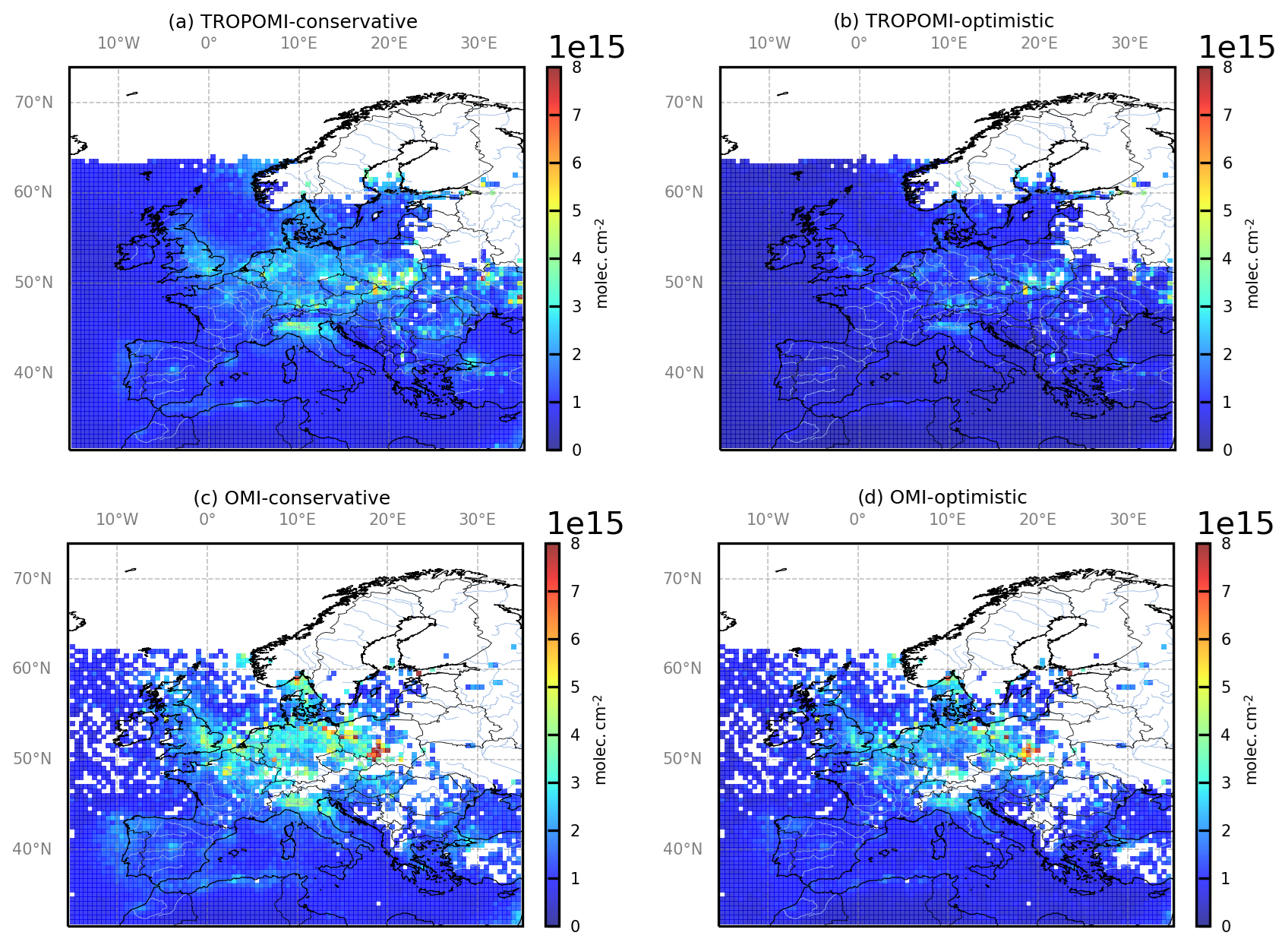
Figure 6 Monthly averages of the observation errors in R for the (a) TROPOMI-conservative, (b) TROPOMI-optimistic, (c) OMI-conservative and (d) OMI-optimistic configurations, in $\mathrm{molec}.{\mathrm{cm}}^{-\mathrm{2}}$, for January 2019. The color scale is the same as for Fig. 7. The observation errors in R include errors corresponding to the satellite retrievals and to the observation operator.

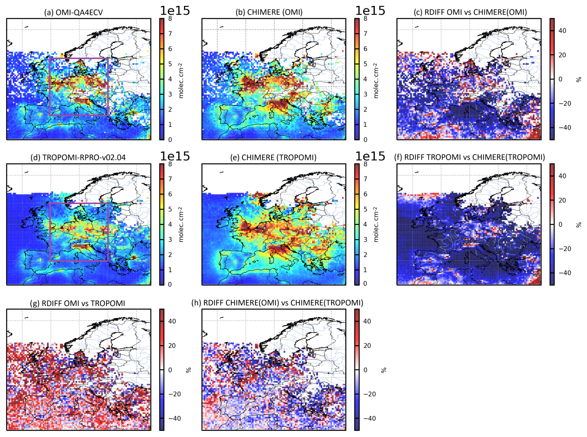
Figure 7 Monthly averages of NO₂ (a) super-observations based on OMI and (b) the CHIMERE-OMI simulation, where and when OMI-QA4ECV super-observations are available, and (d) super-observations based on TROPOMI-RPRO-v02.04 and (e) CHIMERE-TROPOMI simulations, where and when TROPOMI super-observations are available, in $\mathrm{molec}.{\mathrm{cm}}^{-\mathrm{2}}$. Monthly averages for January 2019 of the relative differences between (c) the super-observations from OMI-QA4ECV NO₂ TVCDs and the CHIMERE-OMI simulation, (f) the super-observations from TROPOMI NO₂ TVCDs and the CHIMERE-TROPOMI simulation, (g) the OMI and TROPOMI super-observations, and (h) the CHIMERE-OMI and the CHIMERE-TROPOMI simulations (in %). The prior TNO-GHGco-v3 anthropogenic emissions for the year 2005 are used to simulate the NO₂ TVCDs. The purple box shows western and central Europe (40–60° N, 0–20° E).

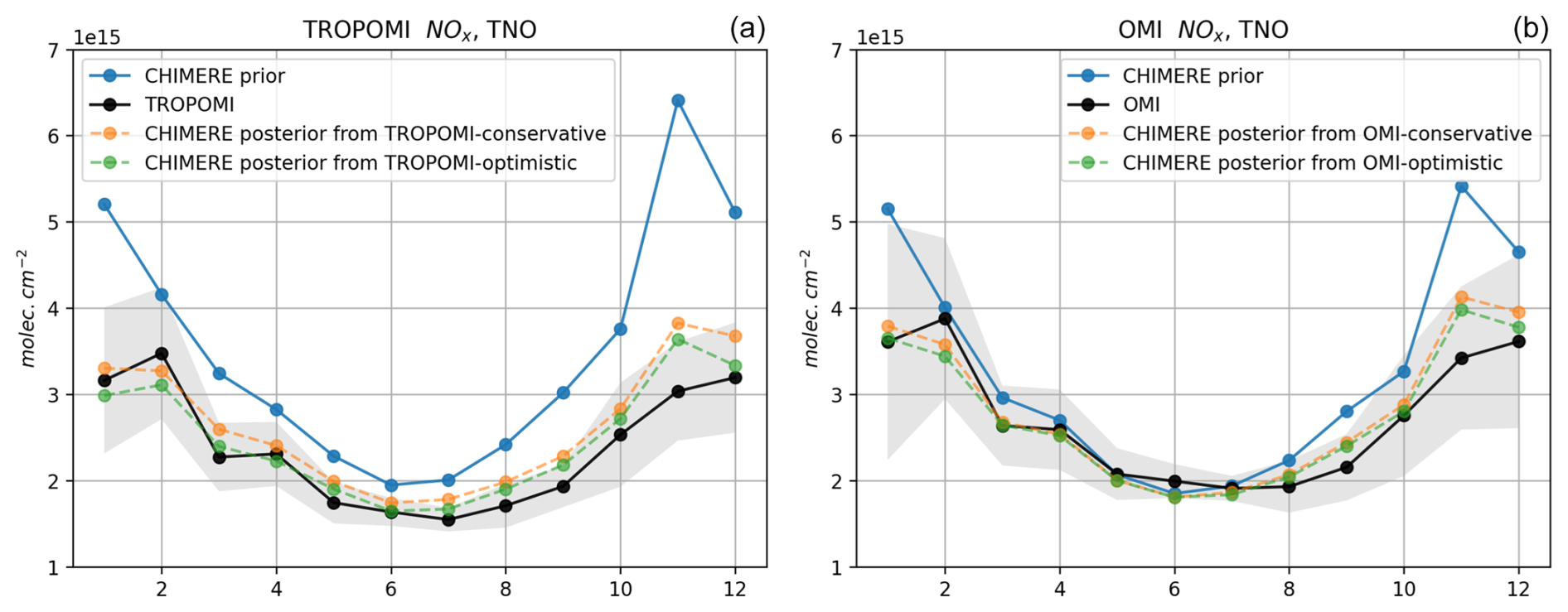
Figure 8 January to December 2019 times series of monthly averaged NO₂ TVCDs over western and central Europe (40–60° N, 0–20° E). (a) From TROPOMI-RPRO-v02.4 super-observations (in black) and the CHIMERE-TROPOMI prior (in blue) and CHIMERE posterior from TROPOMI-conservative (in orange) and CHIMERE posterior from TROPOMI-optimistic (in green) simulations. (b) Same as left but for OMI-QA4ECV super-observations, in $\mathrm{molec}.{\mathrm{cm}}^{-\mathrm{2}}$. The prior simulations of TVCDs use TNO-GHGco-v3 anthropogenic emissions for the year 2005.

OMI NO₂ and TROPOMI NO₂ super-observations present consistent geographical patterns (Fig. 7) with high concentrations over emission hotspots. However, the average magnitude of the NO₂ TVCDs is different. The NO₂ TVCDs in the OMI-QA4ECV product are often higher than in the TROPOMI-RPRO-v02.04 product (Fig. 7a vs. Fig. 7d, Fig. 8), with a mean difference between the two products over the entire domain of about +15 % in January 2019 (Fig. 7g). It could be explained by the fact that TROPOMI underestimates the NO₂ TVCDs over highly polluted areas. The last evaluation of the TROPOMI-RPRO-v02.04 product around the world still indicates significant biases of TROPOMI NO₂ TVCDs of typically +13 % over clean areas to −40 % over highly polluted areas (Lambert et al., 2023; van Geffen et al., 2022b), even if these bias estimates are reduced when MAX-DOAS profile data are vertically smoothed using the TROPOMI AKs.

Since the OMI and TROPOMI AKs are different, and since the spatio-temporal samplings of the two datasets are also different, a direct comparison between the OMI and TROPOMI datasets could be complex or misleading. The confrontation of the OMI retrievals to CHIMERE, on the one hand and of the TROPOMI retrievals to CHIMERE on the other hand can be used as an indirect but more suitable comparison between the OMI and TROPOMI datasets. Interestingly, while the mean NO₂ TVCD observed by OMI is higher by about +15 % than the one observed by TROPOMI, the mean CHIMERE-OMI NO₂ TVCDs are lower by about 7 % compared to the CHIMERE-TROPOMI ones over the entire domain in January 2019 (Fig. 7h). It could be explained by the fact that the AKs in TROPOMI-RPRO-v02.04 tend to be larger above the first four levels than in OMI-QA4ECV (Fig. 3).

3.2 Comparison between satellite super-observations and prior CHIMERE simulations

The CHIMERE-OMI and the CHIMERE-TROPOMI simulations, based on the TNO-GHGco-v3 inventory for the year 2005, both present higher NO₂ TVCDs than the OMI and TROPOMI super-observations for the year 2019 (Fig. 7). This is expected since the NO_x anthropogenic emissions have decreased in Europe since 2005 (EEA, 2021). However, the magnitude of the discrepancies between the simulations and the satellite super-observations varies. For example, in January 2019 over the entire domain, the simulated CHIMERE-TROPOMI TVCDs are about 38 % higher than TROPOMI super-observations, while simulated CHIMERE-OMI TVCDs are about 23 % higher than the OMI ones. Over the most polluted area, including parts of western and central Europe (40–60° N, 0–20° E; see the purple box in Fig. 7), the simulated CHIMERE-TROPOMI and CHIMERE-OMI also present a strong positive relative difference of about +39 % compared to TROPOMI and of about +29 % compared to OMI, respectively. TROPOMI therefore shows a stronger drop in the NO₂ TVCDs than OMI and consequently, the TROPOMI inversions would lead to lower NO_x anthropogenic emissions than the OMI inversions.

The highest differences between the super-observations and the CHIMERE-OMI or CHIMERE-TROPOMI simulations are found in autumn and in winter and particularly for the months of January, November and December (Fig. 8). It can be deduced that the winter European NO₂ simulated TVCDs will be decreased both by the OMI and the TROPOMI inversions, even if the respective corrections to the prior emissions will be different in magnitude. However, in spring and in summer (e.g., for the months of April, May, June, July and August), the monthly averages of the TROPOMI super-observations are always lower than the CHIMERE-TROPOMI NO₂ TVCDs, while the monthly averages of the OMI super-observations remain close to the CHIMERE-OMI ones (Fig. 8b). The TROPOMI and OMI super-observations therefore will lead to different conclusions concerning the potential reductions of NO_x anthropogenic emissions during spring and summer since 2005.

3.3 Improvement of the fit between satellite super-observations and CHIMERE simulations

The inversions bring the simulated NO₂ TVCDs closer to OMI or to TROPOMI super-observations (Fig. 8). In general, the reduction of the bias between the super-observations and the CHIMERE simulations is higher in winter than in summer (Fig. 8). In January 2019 over the entire domain, the mean bias between the TROPOMI super-observations and the CHIMERE-TROPOMI simulations is reduced by about 70 % with the conservative configuration (Sect. 2.4.3), while the mean bias is reduced by about 83 % with the optimistic one. The mean bias between the OMI super-observations and the CHIMERE-OMI simulations is also reduced, by about 73 % with the conservative configuration, while the mean bias is reduced by about 80 % with the optimistic one. The TROPOMI-optimistic and OMI-optimistic corrections are higher than the TROPOMI-conservative and OMI-conservative ones, respectively. It could be explained by the lower error associated with the “optimistic” super-observations, giving more weight to the satellite data, compared to the “conservative” ones (see Sect. 2.4.3).

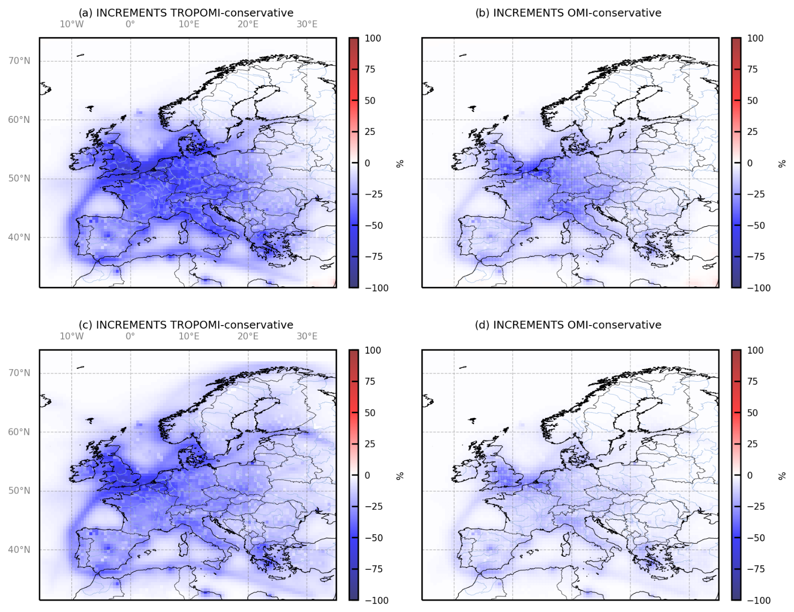
Figure 9 Monthly mean relative corrections to the prior NO_x emissions for year 2005 from the (a) TROPOMI-conservative and from the (b) OMI-conservative inversions, calculated as (posterior − prior) $/$ prior) (in %) for (a, b) the month of January 2019 and (c, d) the entire year 2019.

To improve and optimize the fit between satellite super-observations and CHIMERE simulations, the inversion system reduces the NO_x anthropogenic emissions in the year 2019 (Fig. 9).

3.4 Posterior estimates of NO_x European anthropogenic emissions in 2019: evaluation with comparisons to the TNO-GHGco-v3 inventory

As the anthropogenic emissions contribute to about 95 % of the total NO_x emissions in Europe even in summer (see Sect. 2.3), this section focuses on the inversion results in terms of comparisons between the prior anthropogenic NO_x emissions for 2005 and the posterior emissions from the OMI and TROPOMI inversions for the year 2019 in the European Union + United Kingdom (EU-27 + UK) area. Nevertheless, the inversion results do not seem to indicate missing sources in the biogenic emissions, even if we do not include a specific component of NO_x emissions from agricultural soils in our prior estimate of NO_x emissions (see Sect. 2.2). The annual budget for biogenic emissions is in fact only changed by a few percent by both the OMI and TROPOMI inversions (not shown).

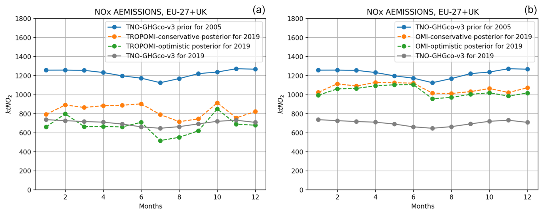
Figure 10 (a) January to December 2019 times series of monthly estimates of anthropogenic NO_x prior emissions from the TNO-GHGco-v3 inventory for the year 2005 (in blue), posterior anthropogenic NO_x emission estimates from the TROPOMI-conservative (in orange) and TROPOMI-optimistic (in green) inversions (in kteq NO₂) for the EU-27 + UK area. (b) Same as left but for posterior anthropogenic NO_x emission estimates from the OMI-conservative (in orange) and OMI-optimistic (in green) inversions.

The posterior emissions from the OMI and TROPOMI inversions are compared to the emission estimates from the TNO-GHGco-v3 inventory for the year 2019 (Table 3, Fig. 10). At the European scale (Fig. 10) and at the national scale (Table 3), both the posterior anthropogenic NO_x emissions from the OMI and TROPOMI inversions for the year 2019 are lower than the prior ones for the year 2005.

Table 2 NO_x anthropogenic emissions for EU-27 + UK estimated from different sensitivity tests described in Table 1 (in kteq NO₂) for the month of January 2005 or for the month of January 2019.

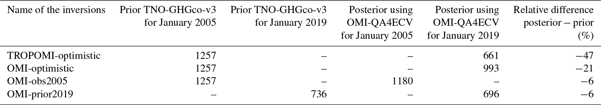
Table 3 National anthropogenic prior NO_x emission estimates from the TNO-GHGco-v3 inventory for the year 2005 and relative increments provided by the different inversions (in %), for the year 2019. The relative differences between emission estimates of the TNO-GHGco-v3 anthropogenic for the year 2019 and year 2005 are given for information.

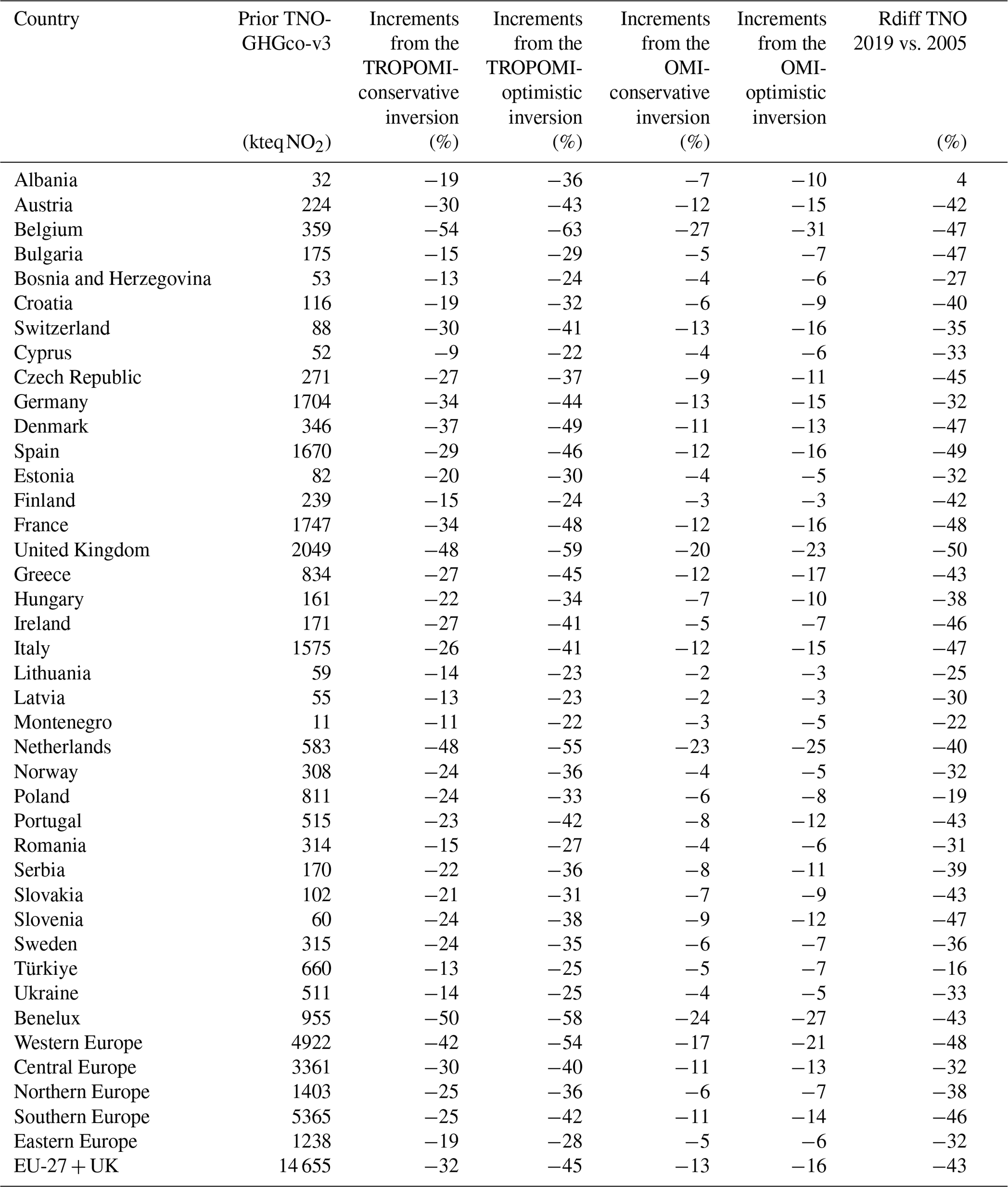
When assimilating OMI-conservative super-observations, the NO_x anthropogenic emissions for EU-27 + UK and for western Europe are decreased by about 13 % and 17 %, respectively, between 2005 and 2019 (Table 3). Similar results are obtained when assimilating OMI-optimistic super-observations (decrease by about 16 % and 21 %, respectively, Table 3). These decreases of emissions between 2005 and 2019 are higher than the decrease estimated by Miyazaki et al. (2017), finding a negative change of only −0.1 % in Europe (defined as 35–60° N, 10° W–30° E in their study) and −8.8 % in western Europe between 2005 and 2014. However, the OMI-conservative and the OMI-optimistic posterior NO_x emissions over EU-27 + UK, respectively, remain +53 % and +47 % higher than the estimation of the TNO-GHGco-v3 inventory for 2019. To support the assumption that the positive bias between the CHIMERE simulations driven by the inventory for 2005 and the satellite observations in 2019 (seen in Fig. 7) is mainly related to the decrease in the European emissions, we have performed two sensitivity tests for the month of January: the first, called “OMI-obs2005”, uses CHIMERE simulations driven by the TNO inventory for 2005 and OMI observations for 2005 (Table 1), and the second, called “OMI-prior2019”, uses CHIMERE simulations driven by the TNO inventory for 2019 and OMI observations for 2019 (Table 1). In these cases, the NO_x anthropogenic emissions for EU-27 + UK in January 2005 and in January 2019 are both decreased by about 6 % by the inversions (Table 2). Using the same configuration of the R covariance matrix, these corrections are much smaller than the correction of about −21 % reached in the case OMI-optimistic for the month of January 2019 (Table 2, Fig. 10), when using prior emissions from the TNO inventory for 2005 and OMI observations for 2019 (Table 1). This result therefore shows that the positive bias between the CHIMERE simulations driven by the inventory for 2005 and the satellite observations in 2019 is mainly due to the decline in European NO_x emissions since 2005.

At the grid-cell scale over both urban and rural areas (Fig. 9) and at the national or European scales (Table 3, Fig. 10), the decreases in NO_x anthropogenic emissions estimated from the OMI inversions between 2005 and 2019 are lower than from the TROPOMI ones. This can be explained by the fact that the relative differences between TROPOMI super-observations and the CHIMERE-TROPOMI simulations are larger than between OMI super-observations and the CHIMERE-OMI ones (see Sect. 3.2), due to different cloud pressures and albedos affecting the averaging kernels (see Sect. 2.4.3). As OMI super-observations are closer to the CHIMERE-OMI simulations, particularly in spring and summer, the OMI inversions make lower corrections in the NO_x anthropogenic emissions than the TROPOMI ones. This can also be explained by the fact that (i) TROPOMI presents a better coverage compared to OMI, with a much larger number of observations (Fig. 5), and (ii) TROPOMI presents lower errors associated with its super-observations than OMI, even in the case where the error associated with the super-observation is not reduced depending on the number of observations (Fig. 6).

Assimilating TROPOMI-conservative super-observations, the decrease in the NO_x anthropogenic emissions for EU-27 + UK and for western Europe between 2005 and 2019 is indeed about −32 % and −42 %, respectively. Assimilating TROPOMI-optimistic super-observations even lead to higher decreases with −45 % and −54 %, respectively, for EU-27 + UK and for western Europe. It could be explained by the lower error associated with the TROPOMI-optimistic super-observations, giving more weight to the satellite data, compared to the TROPOMI-conservative ones (see Sect. 2.4.3). The decrease in NO_x emissions from the TROPOMI-conservative inversions ranges from −9 % for Cyprus to −54 % for Belgium, while it ranges from −22 % for Montenegro to −63 % for Belgium from the TROPOMI-optimistic ones. The TROPOMI-conservative posterior NO_x emissions are closer to the TNO-GHGco-v3 inventory at the European scale compared to the OMI-conservative ones but still with relative differences of about +19 % for EU-27 + UK. The TROPOMI-optimistic posterior emissions become consistent with the TNO-GHGco-v3 inventory, with a relative difference of only −2 %.

Generally, the corrections provided by the inversions are stronger for western and southern countries than for eastern or northern ones (Table 3, Fig. 9). For example, the TROPOMI-optimistic posterior emissions suggest higher annual budgets in several central or eastern European countries (e.g., Slovakia, Slovenia, Croatia) than those provided by TNO, based on official country emission reporting. It may be due to the fact that NO₂ TVCDs (Krotkov et al., 2016; Fortems-Cheiney et al., 2021a) and the NO_x emissions in these countries have not strongly decreased since 2005. It could also be explained by the cloud coverage limiting the number of satellite data over these countries (Fig. 5). When the coverage of a country by OMI or TROPOMI super-observations is sparse, the posterior emissions indeed remain close to the prior emission estimates, i.e., at their 2005 level. Conversely, the TROPOMI-optimistic inversions show lower annual budgets over western European countries such as Belgium and the Netherlands than TNO (Table 3), suggesting that NO_x emissions could have been more reduced than officially reported in these countries.

4 Conclusion

There are great expectations about the detection and the quantification of NO_x emissions using NO₂ TVCDs from satellite observations and inverse systems. This study assesses the potential of the OMI-QA4ECV and TROPOMI satellite observations to improve the knowledge on European NO_x emissions at the regional scale and to inform about the spatio-temporal variability of NO_x emissions in 2019 compared to 2005, at the resolution of 0.5° over Europe. Starting from European emission estimates from the TNO-GHGco-v3 inventory for the year 2005, regional inversions using the CIF coupled to CHIMERE CTM and assimilating satellite NO₂ TVCDs from OMI and TROPOMI have been performed to estimate the European annual and seasonal budgets for the year 2019.

As the anthropogenic emissions strongly contribute to the total NO_x emissions in Europe even in summer, we assume that the differences between the 2005 and the 2019 budgets are mainly due to anthropogenic emissions and not to the biogenic ones. However, the level of distinction between the anthropogenic and biogenic emissions in the inversions is one of the sources of uncertainty in the estimate of the anthropogenic emissions. The corrections provided by the inversions to the prior emissions can also be limited by the cloud coverage affecting the OMI or TROPOMI observations, by errors in the OMI or TROPOMI data, and by errors in the CTM. Finally, the setup of error covariance matrices could also have a strong impact on the emission estimates resulting from the inversions.

Both the OMI and TROPOMI inversions show decreases in European NO_x anthropogenic emission budgets in 2019 compared to 2005. Nevertheless, the magnitude of the reductions of the NO_x anthropogenic emissions is different with OMI and TROPOMI data, with decreases in EU-27 + UK between 2005 and 2019 of 16 % and 45 %, respectively. The decrease in NO_x anthropogenic emissions estimated from the TROPOMI inversions is substantially higher than from the OMI inversions. This is mainly explained by (i) the fact that the differences between CHIMERE-TROPOMI simulations and the TROPOMI super-observations are larger than between CHIMERE-OMI and OMI super-observations, due to different AKs; (ii) the better coverage of TROPOMI compared to OMI; and (iii) the lower errors associated with the TROPOMI super-observations compared to OMI.

The TROPOMI-optimistic inversions, giving weight to the satellite data, become consistent with the independent TNO-GHGco-v3 inventory for the year 2019, with annual budgets for EU-27 + UK showing absolute relative difference of only 2 %. These TROPOMI inversions are therefore in agreement with the magnitude of the decline in NO_x emissions declared by countries, when aggregated at the European scale.

Our results, with OMI and TROPOMI data but also with different choices made for the derivation of the error associated with each super-observation, lead to different magnitudes of corrections on NO_x anthropogenic emissions. This suggests that more observational constraints and further work would be required to sharpen the European emission estimates. Observational information from future satellite missions such as Sentinel-4 on board geostationary satellites would increase the number of observations for better constraining the NO_x emissions in particular for eastern and northern countries. However, even if considering the corresponding increase in the observation sampling and weight, there is a particular need for in-depth analysis of the spatial correlations of the error components in the TROPOMI and OMI NO₂ TVCD retrievals to support the configuration of the errors on super-observations, as recently highlighted by Rijsdijk et al. (2025).