Shallow cloud variability in Houston, Texas, during the ESCAPE and TRACER field experiments

Shallow convection plays an important role in Earth's climate system by regulating the vertical transport of heat, moisture, and momentum in the lower troposphere. Aerosols, large-scale meteorology, and low-level convergence influence the spatiotemporal variability in shallow convection, and the coastal urban area of Houston, Texas, is an ideal laboratory to investigate these complex interactions. Here, geostationary satellite and ground-based radar observations from June to September 2022 during the TRacking Aerosol Convection interactions ExpeRiment (TRACER) and Experiment of Sea Breeze Convection, Aerosols, Precipitation, and Environment (ESCAPE) field campaigns are used to characterize the spatial coverage, vertical extent, and precipitation fraction of shallow convective clouds. The fused operational remote sensing datasets over a 250 km × 250 km domain are evaluated against profiling observations. The domain-wide diurnal shallow cloud fractions are used to identify four distinct modes of shallow convection. In all clusters, the domain-wide cloud fractions are consistently higher than the domain-wide precipitation fractions, and shallow cloud fractions are higher over water than they are over land, while the shallow precipitation fractions show the opposite behavior. In the two modes with minimal deep cloud activity, shallow cloud frequency is highest over ocean in the early morning, and there is a transition to higher shallow cloud frequency over land by the afternoon in one cluster or to high shallow cloud frequencies everywhere by the afternoon in the other. Lastly, we find regions with higher shallow cloud top heights and a large region along the coastline where shallow clouds are more likely to precipitate.

1 Introduction

Atmospheric convection is a fundamental mechanism for the vertical transport of heat, moisture, and momentum in the troposphere, significantly impacting the large-scale atmospheric circulation and local environment. Convection also modulates cloudiness, which further influences large-scale atmospheric circulations (Hartmann et al., 1984; Su et al., 2014; Sherwood et al., 2014). Several factors contribute to the formation, evolution, and dissipation of convective clouds, including aerosols, large-scale meteorology, and boundary layer organization (Rosenfeld et al., 2006, 2008; Fan et al., 2013; Varble, 2018; Lebo, 2018; Wilson and Schreiber, 1986). A coastal urban area like Houston, Texas, is an excellent place to observe all of the complicated interactions between convection, aerosols, large-scale meteorology, and convergence zones (Jensen et al., 2022). In particular, the Houston region is warm and humid in the summer and commonly experiences onshore flow and sea-breeze-forced convection (Fridlind et al., 2019), which interacts with a range of aerosol conditions associated with the city's urban and industrial emissions. This argument was initially put forward by the Aerosols, Clouds, Precipitation, and Climate (ACPC) work group, a joint initiative of the International Geosphere–Biosphere Programme and the World Climate Research Programme (Quaas et al., 2015). This effort led to the organization of two large field experiments in the Houston area during the 2022 summer period. The National Science Foundation (NSF) sponsored the experiment entitled “Experiment of Sea Breeze Convection, Aerosols, Precipitation, and Environment” (ESCAPE; Kollias et al., 2024), which took place between 30 May and 30 September 2022. ESCAPE aimed to characterize the life cycles of convective cloud dynamics in a coastal urban environment with prominent aerosol sources (Jensen et al., 2022). It coincided with the same 4-month intensive observation period (IOP) of the United States Department of Energy (DOE) Atmospheric Radiation Measurement (ARM)-funded “TRacking Aerosol Convection interactions ExpeRiment” (TRACER; Jensen et al., 2022) field campaign. TRACER focused on quantifying the impact of aerosols on convective clouds properties such as updraft strength, microphysical properties, and cloud and precipitation coverage.

There is growing body of observational work coming from these field experiments. During TRACER, Wang et al. (2024) identified 46 sea breeze events and the anticyclonic synoptic conditions that favor their development; they found that these events induce updrafts in the boundary layer which likely promote the formation of isolated deep convective precipitating cores that have short lifetimes and mostly exist near the coast. Similarly, Sharma et al. (2024) quantified the impact of air mass heterogeneity across sea and bay breeze fronts on 15 IOP days' worth of shallow and transitioning convective clouds, and they showed that air mass heterogeneity has a more noticeable impact on the bulk microphysical properties of their shallow cloud sample. Finally, Bruning et al. (2024) tracked the radar and lightning characteristics of ∼7500 thunderstorms during the period, and they showed that storms with lightning had more pronounced polarimetric signatures, showcasing lightning as a useful tool for understanding mixed-phase precipitation processes in the region.

A study focusing on a large sample of warm-phase (shallow) convective properties would greatly complement the results of these recent studies. Shallow cumulus clouds are the most frequently observed cloud type in the Houston area compared to deep convective clouds (Tuftedal et al., 2024). While most of the previous studies focused on deep convection in this area, precipitation from shallow convection is non-negligible in terms of the total precipitation in the area (Kumar et al., 2013a, b). Especially in humid environments, even shallow convective clouds can produce heavy precipitation with comparable radar reflectivities to deep convection (May and Ballinger, 2007; Oue et al., 2010). Furthermore, shallow convection can modulate the lower atmosphere by moistening it, which favors the subsequent development of deep convection (Sherwood and Wahrlich, 1999; Derbyshire et al., 2004; Mapes et al., 2006; Holloway and Neelin, 2009; Nuijens et al., 2009; Powell and Houze, 2013). Aerosol–cloud interactions on shallow convective clouds have been studied since the 1970s. While they have established the impact of aerosols on droplet number concentrations and sizes (e.g., Twomey, 1974; Lohmann and Feichter, 2005), much less has been reported in terms of invigoration (depicted as deepening of the shallow cloud layer) or precipitation modulation. Thus, it is not well understood what environments, including meteorological, aerosol, and geographical conditions, control the early growth stage of convective clouds.

In this paper, operational satellite and weather radar datasets are combined to provide a large statistical sample of precipitating and nonprecipitating clouds over the Houston area during the 4-month ESCAPE and TRACER period. Daily statistics are used to infer the different spatiotemporal patterns of both shallow and deep convective clouds, and comparisons over land and ocean are used to further elucidate the relationships between clouds, precipitation, surface type, and meteorology. The main objective of this paper is therefore to characterize the spatiotemporal variability in shallow clouds and their associated precipitation patterns. Four main diurnal characteristics of shallow clouds will be evaluated over land and water: cloud fraction, frequency of occurrence, cloud top height, and precipitation occurrence.

2 Data

2.1 DOE ARM observations

During the TRACER field campaign, the DOE ARM program deployed the first ARM Mobile Facility (AMF1) at La Porte Municipal Airport, located 35 km east of the Houston downtown area (29°40^′12^′′ N, −95°3^′32.4^′′ E). The AMF1 operates a comprehensive suite of active and passive remote sensors that can provide continuous, high-spatiotemporal-resolution information about aerosols, clouds, precipitation, and radiation in the atmosphere above and around the AMF1 site. For example, the Parsivel2 laser disdrometer at the AMF1 measures particle size distribution over the range of 0.06–24 mm and classifies precipitation type (liquid and frozen) using the precipitation rate (Wang and Bartholomew, 2023). Precipitation type and rate are used here (Wang and Shi, 2021). In addition, frequent radiosonde launches were performed at the AMF1 site. The TRACER campaign followed a schedule of four radiosonde launches per day at 6 h intervals (approximately 00:00, 06:00, 12:00, and 18:00 UTC), but this schedule varied slightly on “enhanced sounding days” with forecasted deep convection. On these days, an additional radiosonde was launched at approximately 21:00 UTC to better capture the rapid daytime development of the atmospheric thermodynamic structure (Jensen et al., 2019). Vertical profiles of atmospheric state variables like pressure, temperature, relative humidity, wind speed, and wind direction collected by the radiosondes are used here (Burk, 2021).

Value-added products (VAPs), which provide post-processed data from the suite of instruments at the AMF1, are also available. The Active Remote Sensing of Clouds (ARSCL; Clothiaux et al., 2001; Kollias et al., 2016) VAP combines profiling millimeter-wavelength radar and lidar observations to estimate a feature mask that includes the moments of the Doppler spectrum and cloud boundary estimates from laser ceilometers and micropulse lidars (MPLs). The Ka-band zenith-pointing radar (KAZR; Kollias et al., 2020b) is the profiling millimeter-wavelength radar operating at the AMF1 during TRACER, and it has a vertical resolution of 30 m and a temporal resolution of 2 s. The KAZR radar reflectivity and cloud base height estimate from ARSCL are used here (Johnson et al., 2021).

2.2 KHGX WSR-88D observations

The Next Generation Weather Radar (NEXRAD) network, a joint effort between the United States Department of Commerce, Department of Defense, and Department of Transportation (Crum and Alberty, 1993), operates about 160 S-band Doppler dual-polarization radars across the country to provide consistent, high-resolution surveillance of weather phenomena for meteorologists and decision-makers. These radars have a range resolution of 250 m; an azimuthal resolution of 1°; and, depending on the volume coverage pattern (VCP), a range of temporal resolutions from 4–10 min (Interagency Council for Advancing Meteorological Services, 2011). The Weather Surveillance Radar-1988 Doppler (WSR-88D) system responsible for monitoring the Houston, Texas, and Galveston, Texas, metropolitan areas is located 35 m above mean sea level in Dickinson, Texas, at 29°28^′18.84^′′ N, 95°04^′43.82^′′ W (Interagency Council for Advancing Meteorological Services, 2011). It is given the identifier KHGX. KHGX operated in clear-air mode, using VCPs 31, 32, and 35, and in precipitation mode, using VCPs 21, 212, and 215, in the 4 months of interest.

During the TRACER and ESCAPE IOPs, the KHGX observations were processed in real time to support the operation of the Multisensor Agile Adaptive Sampling (MAAS; Kollias et al., 2020a; Lamer et al., 2023) algorithm implanted in the second-generation C-band scanning ARM precipitation radar (CSAPR2; Kollias et al., 2020b) and the Colorado State University C-band Hydrological Instrument for Volumetric Observation (CHIVO) radar to conduct convective cell tracking (Lamer et al., 2023; Kollias et al., 2024). The three-dimensional KHGX data (two dimensions in azimuth and one dimension in elevation) were first quality-controlled for nonmeteorological echoes and then interpolated onto a horizontal Cartesian grid for comparison with satellite data. These gridded and masked data were then used to construct a 1.5 km above ground level (a.g.l.) constant-altitude plan position indicator (CAPPI; Douglas, 1990) and a map of vertically integrated liquid (VIL) in the domain. VIL is estimated using the Marshall–Palmer drop size distribution assumptions (Marshall and Palmer, 1948):

$$\begin{array}{}\text{(1)}& \text{VIL}=\sum _{i=\mathrm{0}}^{\text{top}}\mathrm{3.44}\times {\mathrm{10}}^{-\mathrm{6}}{\left[{\displaystyle \frac{Z_i+Z_{i+\mathrm{1}}}{\mathrm{2}}}\right]}^{\mathrm{4}/\mathrm{7}}\mathrm{\Delta }h,\end{array}$$

where Z stands for radar reflectivity (in dBZ) and Δh stands for the depth of the layer between consecutive grid levels (in m). More specific details on these processes can be found in Lamer et al. (2023). For this study, we use the KHGX CAPPI, VIL, and three-dimensional data.

2.3 GOES-R ABI observations

The Geostationary Operational Environmental Satellite-R Series (GOES-R) is the National Oceanic and Atmospheric Administration's (NOAA) latest generation of satellites, providing users with continuous, high-resolution data to assist with weather forecasting, storm tracking, and atmospheric research (National Aeronautics and Space Administration, 2019). The Advanced Baseline Imager (ABI) is one of the key instruments on GOES-R and provides radiance data in 16 spectral bands/channels ranging from the visible part of the electromagnetic spectrum to the near-infrared and the infrared. Of interest here, Channel 2 sits in the wavelength range of 0.59–0.69 µm and has an instantaneous field of view (IFOV) of 0.5 km and a temporal resolution of 5 min (Schmit et al., 2005; Schmit et al., 2018), which is useful for studying fog, anvils, cumulus clouds, and ice and/or snow cover amongst phenomena. Channel 13 sits in the wavelength range of 10.1–10.6 µm and has an IFOV of 2 km and a temporal resolution of 5 min (Schmit et al., 2005, 2018), and it is useful for studying atmospheric moisture, performing cloud identification and classification, estimating cloud top temperature and particle size, and characterizing surface properties (Lindsey et al., 2012). Specifically, this study uses the reflectance data from Channel 2 to identify cloud presence and the brightness temperature data from Channel 13 to identify cloud phase.

The ABI Cloud Mask (hereafter ACM) product combines 9 of the 16 bands to provide a binary classification of “cloudy” or “clear” for each pixel using spectral, spatial, and temporal signatures and has a horizontal resolution of 2 km and a temporal resolution of 5 min (Heidinger and Straka, 2013). We make use of the four-level version of the mask which provides a classification of “cloudy”, “probably cloudy”, “probably clear”, or “clear” for each pixel.

2.4 HRRR data

The High-Resolution Rapid Refresh (HRRR; James and Benjamin, 2017; Dowell et al., 2022; James et al., 2022) is run by NOAA and National Centers for Environmental Prediction (NCEP), and it is the convection-allowing implementation of the Advanced Research version of the Weather Research and Forecasting (WRF-ARW; Skamarock et al., 2019) model. HRRR has 3 km spatial resolution and 51 vertical levels, hourly data assimilation, and hourly forecasts for the continental United States. Boundary conditions are provided by the HRRR system. We acquired the hourly HRRR files using the Herbie Python library (Blaylock, 2024), and we use 850 hPa temperature, relative humidity, wind speed, and wind direction from model analysis at forecast hour 0 here.

3 Methodology

3.1 Observational domain

The analysis domain size is 250 km × 250 km centered at KHGX. In terms of spatial extent, the southwestern-most point of the domain is 28°20^′35.8794^′′ N, 96° 21^′16.56^′′ W, and the northeastern-most point of the domain is 30°35^′17.16^′′ N, 93°46^′31.08^′′ W. Figure 1a shows the domain, with the KHGX site located southeast of the city of Houston and the AMF1 located northeast of the radar location and southeast of the city. The KHGX and GOES-R data are gridded onto a horizontal Cartesian grid using a K-D tree interpolation algorithm at a 500 m grid spacing (Bentley, 1975).

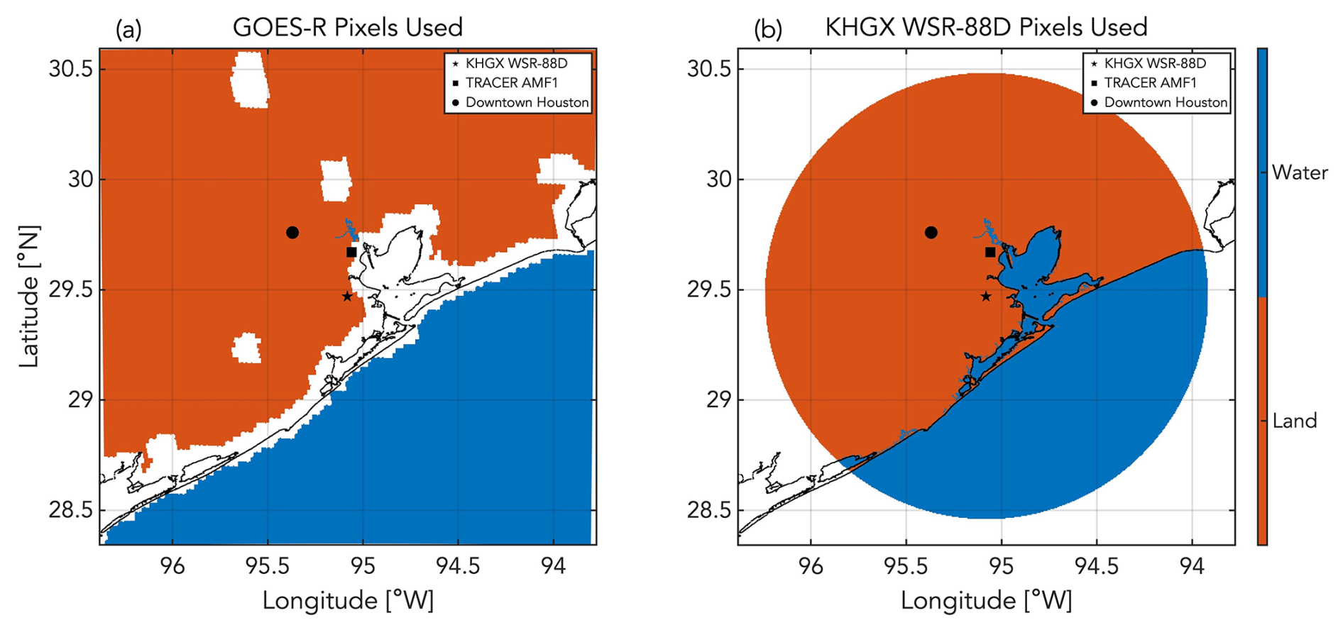
Figure 1 For the 250 km × 250 km grid used in this study, the map of the pixels classified as land (orange) and water (blue) used in (a) the GOES-R ABI data and (b) the KHGX WSR-88D data. The pixels included in panel (b) are constrained to the region within the 225 km diameter range ring. The locations of the TRACER AMF1, the KHGX WSR-88D, and downtown Houston are indicated by a square marker, a star marker, and a circle marker, respectively.

An important methodology step is to consider limitations of the operational GOES-R and KHGX observations that will affect the cloud and precipitation analysis. A preliminary perusal of the GOES-R ABI Cloud Mask (ACM) indicated a noticeable suppression of cloud detections in the grid points around the coastline of Houston compared to the surrounding areas. The surface properties (reflectance and emissivity) play a key role in the ACM performance, and this affects the ACM statistics in the areas where there is surface type transition (i.e., water to land) near the coastlines and waterbodies over land. As a result, the grid points that correspond to these areas (white areas in Fig. 1a) are ignored in further analysis of the GOES-R observations. Overall, 135 994 (87.5 %) of the land grid points and 81 202 (85.9 %) of the water grid points are used here. The coverage, resolution, and sensitivity of the KHGX observations depend on distance from the radar (Kollias et al., 2022). As a result, the 1.5 km CAPPIs show artifacts generated by the fact that only one elevation angle (the lowest) provided coverage at this height a.g.l. Thus, we have limited the KHGX analysis to the region within the 225 km diameter range ring (Fig. 1b). Overall, 102 490 (65.9 %) of the land grid points and 56 311 (59.6 %) of the water grid points are used here.

3.2 Comparison of KHGX WSR-88D, GOES-R ABI, and DOE ARM observations

The study of the cloud and precipitation spatiotemporal patterns presented in this study is based on the KHGX and GOES-R sensor fusion. The AMF1 provides a unique opportunity to evaluate the ability of the GOES-R ACM to detect clouds and the ability of the KHGX to detect light precipitation. Previous studies have assessed the cloud mask's skill using other satellite measurements (Jimenez, 2020; McHardy et al., 2022), but, to our knowledge, a verification using ground-based measurements has never been conducted. An example of collocated KHGX, GOES-R, and ARM observations is shown in Fig. 2. Figure 2 shows a time–height plot of KHGX observations over the AMF1 location using KHGX radar reflectivity data collected at different elevation angles. The ARSCL cloud layer boundaries and the KAZR radar reflectivity are shown in Fig. 2b. Finally, the corresponding GOES-R ABI reflectance data from Channel 2 and the brightness temperature data from Channel 13 are shown in Fig. 2c.

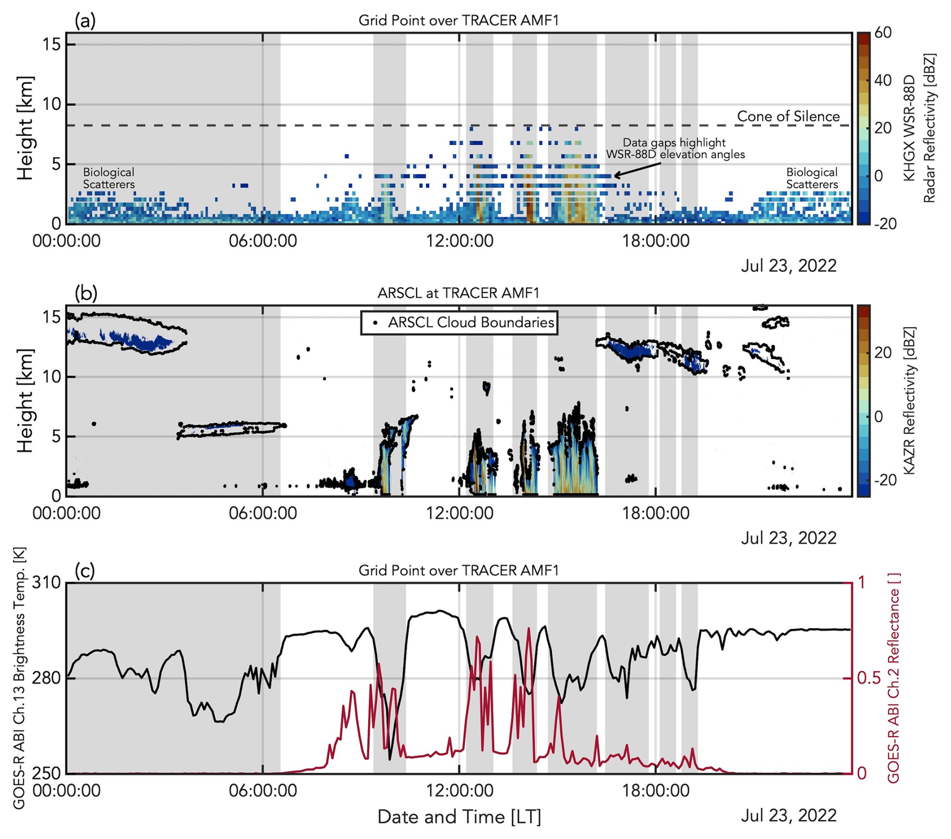
Figure 2 On 23 July 2022, (a) time–height mapping of KHGX WSR-88D radar reflectivity at all 15 elevation angles (running in VCP A215 for most of the day: 0.5, 0.9, 1.3, 1.8, 2.4, 3.1, 4, 5.1, 6.4, 8, 10, 12, 14, 16.7, and 19.5°) in the 0.5 km × 0.5 km grid point over the TRACER AFM1 site, (b) time–height mapping of KAZR radar reflectivity (color) and cloud boundaries (black points) from the ARSCL product at the TRACER AMF1, and (c) time–height mapping of GOES-R ABI Channel 13 brightness temperatures (black) and GOES-R ABI Channel 2 reflectance (red) in the 0.5 km × 0.5 km grid point over the TRACER AMF1. Gray shading indicates the periods when the GOES-R ABI Cloud Mask has values of “cloudy”.

Between 00:00 and 06:00 LT on 23 July 2022, the GOES-R ACM accurately reports the presence of thin cirrus clouds identified in the ARSCL data (Fig. 2b). The cirrus clouds' low radar reflectivity and high altitude make them impossible to be detected with the KHGX WSR-88D due to the radar's limited sensitivity and the limit in the maximum height of the radar observations (dashed line in Fig. 2a) imposed by the maximum elevation angle of the radar and its distance from the AMF1 site. Overall, there is good correspondence, in terms of cloud presence and duration, between the ACM and the cloud/precipitation and clear conditions as captured by KHGX and ARSCL observations. The “cloudy” periods show increases in radar reflectivity in both radars, increases in reflectance, and decreases in brightness temperature (Fig. 2). The comparison between KAZR and KHGX also shows the value a WSR-88D can provide in representing a cumulus cloud's morphology (width, cloud top height, etc.) despite its usage for operational surveillance. A more comprehensive assessment of the ACM is provided in Appendix A.

A notable feature in Fig. 2a is the radar reflectivity echoes present in the lowest 3 km during 00:00–03:00 and 21:00–23:00 LT; these are nonmeteorological echoes associated most likely with biological activity. It is important to consider that WSR-88Ds are sensitive not only to hydrometeors (precipitation) but also to Bragg scattering and insects (Melnikov et al., 2011). There is also a consistent presence of radar reflectivity echoes in the lowest 1 km throughout the day due to ground clutter. Although not a perfect one-for-one comparison, the ARSCL data do not show these features and certainly do not have any strong precipitation echoes at the times noted (Fig. 2b). This is why the vigorous quality control was done in Lamer et al. (2023) when creating the 1.5 km CAPPI and VIL datasets. To ensure we are only examining hydrometeors, we use a VIL threshold of 0.1 kg m⁻² throughout the study like Lamer et al. (2023) did.

We then use the AMF1 measurements to determine the lowest KHGX radar reflectivity value applicable across the domain to detect the presence of precipitation in cumulus clouds. The AMF1 surface disdrometer observations over the 4-month IOP are used to characterize the precipitation types and their frequency of occurrence at the observatory. Measured surface precipitation, which includes all weather codes associated with drizzle and rain, is observed 2.26 % of the time (not shown). To compare, the KHGX 1.5 km CAPPI radar reflectivity values over the AMF1 site are used to estimate the frequencies of individual radar reflectivity values, and we find that the most frequently occurring radar reflectivity values over the site are between 10 and 30 dBZ (Fig. 3a). We also calculate the cumulative frequency of occurrence of radar reflectivity thresholds between −10 and 60 dBZ, meaning we calculate the frequency with which values greater than a threshold on the x axis occur during the period (Fig. 3b). We find that a KHGX 1.5 CAPPI radar reflectivity threshold of 7.5 dBZ matches the frequency of occurrence of measured surface precipitation by the disdrometer at the AMF1. The 7.5 dBZ radar reflectivity threshold is subsequently used to derive the diurnal variability in precipitation over the AMF1 site, and it is compared to the diurnal variability in precipitation by the AMF1 disdrometer (Fig. 3c). They show strong agreement, and both measure the maximum occurrences between 12:00 and 18:00 LT and the secondary maxima in the late evening and early morning hours (Fig. 3c).

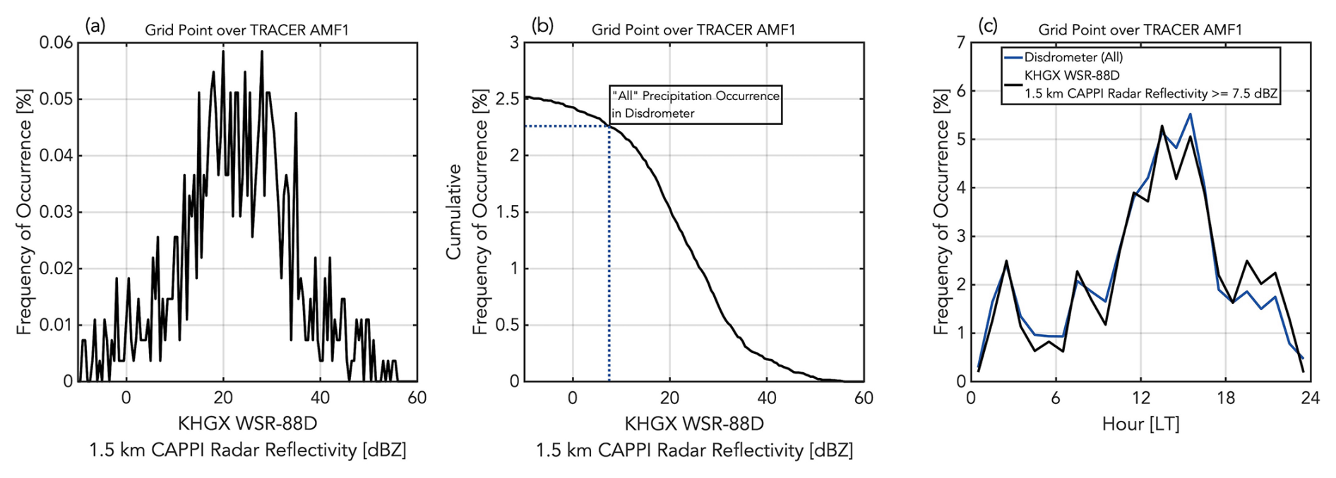
Figure 3 From 1 June–30 September 2022, (a) the frequency of occurrence of individual radar reflectivity values in the KHGX WSR-88D 1.5 km CAPPI radar reflectivity data for the 0.5 km × 0.5 km grid point over the TRACER AMF1, (b) the frequency of occurrence of cumulative “greater than or equal to” radar reflectivity thresholds in the KHGX WSR-88D 1.5 km CAPPI radar reflectivity data for the 0.5 km × 0.5 km grid point over the TRACER AMF1, and (c) the frequency of occurrence every hour of all precipitation (drizzle and rain) from the disdrometer at the TRACER AMF1 (blue) and of radar reflectivity values greater than or equal to 7.5 dBZ in the KHGX WSR-88D 1.5 km CAPPI radar reflectivity data for the 0.5 km × 0.5 km grid point over the TRACER AMF1 (black).

One final consideration is that KHGX's sensitivity is inversely proportional to the square of the radar range. Before using the 7.5 dBZ radar reflectivity threshold, we confirm that it is above KHGX's minimum detectable signal at far ranges (as depicted in the 1.5 km a.g.l. CAPPI data) and that it is above any Bragg scattering returns. At the furthest range considered in this study (112.5 km from KHGX), the minimum detectable signal is between 0 and 5 dBZ, so our threshold is applicable. This means, using the conversion of the KHGX radar reflectivity to rainfall rate (R) in this climatological regime provided by the National Weather Service (R=300Z^1.4; Battan, 1973), we detect rainfall rates as low as 0.058 mm h⁻¹ in our domain. So, for the rest of our analysis, the pixels in our KHGX dataset must exceed a 1.5 km CAPPI radar reflectivity of 7.5 dBZ and a VIL of 0.1 kg m⁻² to be classified as precipitation.

3.3 Shallow and deep cloud and precipitation classification

An example of the cloud and precipitation classification during an ESCAPE aircraft IOP on 2 June 2022 at 11:22:36 LT is shown in Fig. 4. The GOES-R ACM data are used to define clear and cloudy conditions (Fig. 4b). The GOES-R Channel 13 brightness temperature data (T_B13) in Fig. 4a show widespread shallow cloudiness across the domain, except a small region south and east of Galveston Bay where colder T_B13 is observed. The T_B13 values are used to further classify the clouds identified in the GOES-R ACM data as warm phase only if $T_{\text{B13}}>-\mathrm{5}\mathrm{°}\mathrm{C}$, at which point it is reasonable to assume there is no ice present, and as mixed phase only if $T_{\text{B13}}<-\mathrm{5}\mathrm{°}\mathrm{C}$. The cloud top height and temperature are strongly related; thus, the warm-phase-only clouds are hereafter called shallow convection and the mixed-phase clouds are called deep convection (Fig. 4c and d). In addition, the gridded KHGX CAPPI data are used to classify the detected clouds as precipitating or not (Fig. 4f–h). We use the radar reflectivity and VIL thresholds described above, and we classify each pixel as shallow or deep by comparing the highest KHGX echo top height (no reflectivity threshold considered) at that pixel to the median height of the −5 °C level (5.79 km; not shown) derived from the AMF1 soundings, where a radar echo top height less than 5.79 km is shallow and greater than 5.79 km is deep. At this instance in time, the shallow clouds over the gulf (Fig. 4c) are not precipitating (Fig. 4g) from the radar's perspective, while more of the shallow clouds along the coastline and over land are in fact precipitating. There is a prominent cold top feature east of Galveston Bay (Fig. 4d) with some deep precipitation associated with it (Fig. 4h). Otherwise, this instance in time is defined by more shallow cloud and precipitation features, with abundant activity along the coastline.

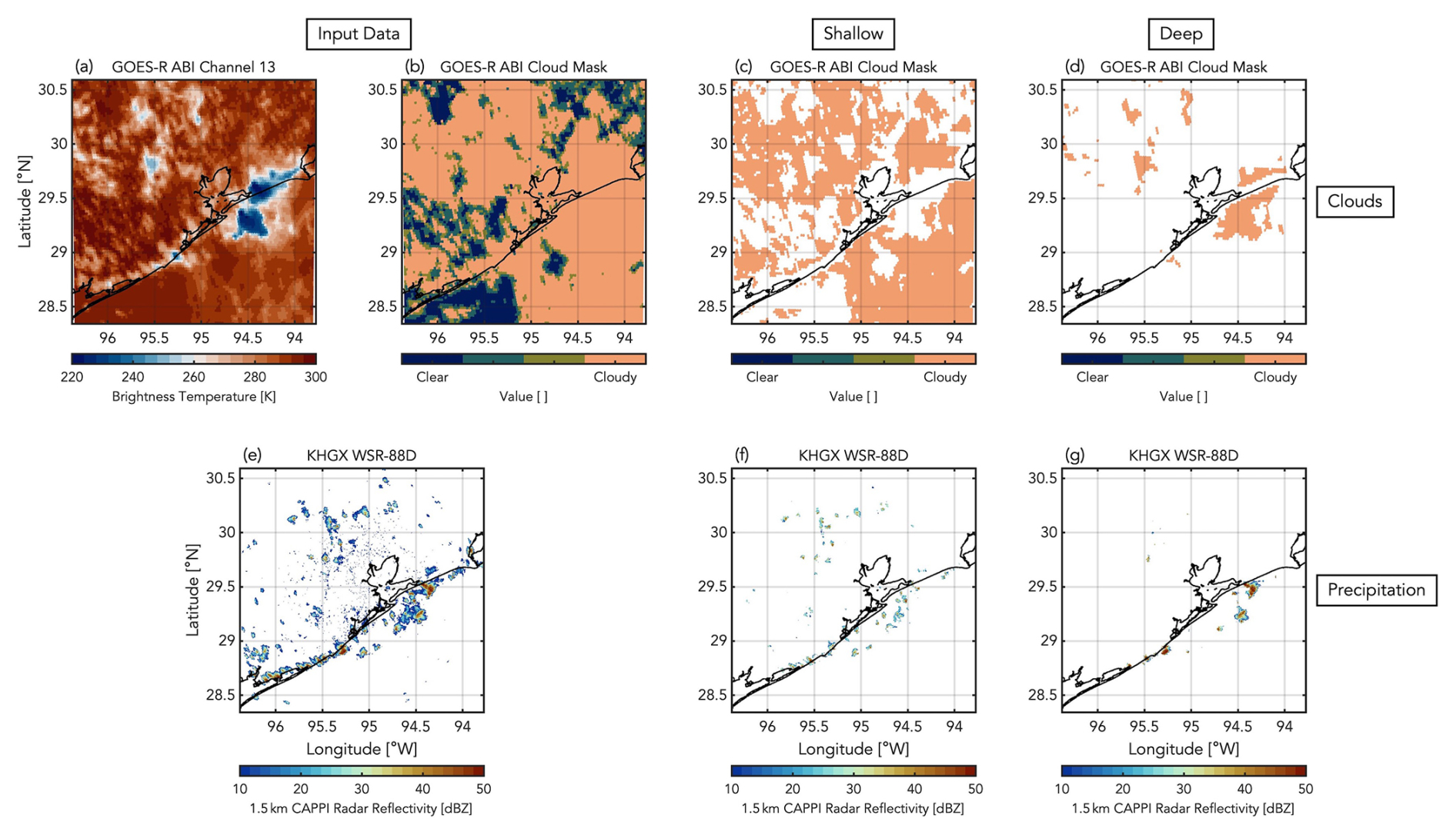
Figure 4 On 2 June 2022 at 11:22:36 LT, (a) GOES-R ABI Channel 13 brightness temperatures, (b) GOES-R ABI Cloud Mask values, (c) GOES-R ABI Cloud Mask warm-phase cloudy pixels, (d) GOES-R ABI Cloud Mask mixed-phase cloudy pixels, (f) KHGX WSR-88D 1.5 km CAPPI radar reflectivity values, (g) KHGX WSR-88D 1.5 km CAPPI radar reflectivity values associated with warm-phase echo tops, and (h) KHGX WSR-88D 1.5 km CAPPI radar reflectivity values associated with cold-phase echo tops.

An important consideration for this approach is that the satellite will report the brightness temperature of the coldest (highest) feature at that pixel. This means that a deep cloud pixel could be a cirrus cloud, an anvil, or a deep convective cumulus cloud, and we do not make any sort of classification. These features may also obscure shallow clouds beneath them, leading to an underrepresentation of shallow clouds in environments with deep cloud activity. In the subsequent analysis, we report all shallow and deep cloud activity, but we will eventually focus on periods with minimal deep cloud activity to avoid underrepresenting the shallow clouds we are scientifically interested in.

4 Results

4.1 Domain-averaged diurnal cycle of clouds and precipitation

The gridded KHGX radar and GOES-R data products are used to estimate the fraction of the analysis domain covered by warm (shallow) and cold (deep) cloud tops. We calculate the number of shallow cloud, deep cloud, shallow precipitation, and deep precipitation pixels and divide by the total number of pixels in the domain used for each instrument. The domain-averaged fractions are estimated approximately every 5 min, and their median value within an hour is used to derive the diurnal variability in shallow and deep clouds throughout the 4-month TRACER and ESCAPE IOP period (Fig. 5). The maximum hourly median shallow cloud fraction in the dataset is 84.2 % at 09:00 LT on 8 June; meanwhile, the maximum hourly median deep cloud fraction in the dataset is 100 % at 15:00 LT on 4 September. Of the 121 d that are not missing data, 37 have their maximum hourly median shallow cloud fraction occur between 00:00 and 05:00 LT, 13 have their maximum occur between 06:00 and 11:00 LT, 31 have their maximum occur between 12:00 and 17:00 LT, and 40 have their maximum occur between 18:00 and 23:00 LT. Similarly, of the 112 d that are not missing data and that have hourly median deep cloud fractions above 0 % all day, 19 have their maximum hourly median shallow cloud fraction occur between 00:00 and 05:00 LT, 12 have their maximum occur between 06:00 and 11:00 LT, 44 have their maximum occur between 12:00 and 17:00 LT, and 37 have their maximum occur between 18:00 and 23:00 LT. Indicated by these statistics, the morning hours of 06:00–11:00 LT experience the maximum hourly median shallow and deep cloud fractions least frequently, and the maximum hourly median shallow cloud fraction occurs most frequently in the evening, while the maximum hourly median deep cloud fraction occurs most frequently in the afternoon. Overall, the domain-averaged fractional coverage of shallow clouds indicates that they are more frequently observed than deep clouds in the domain throughout the period. The domain-averaged shallow cloud fraction is always above 0 %, while 9 d has no observable deep clouds in the domain. Likewise, the maximum hourly median shallow cloud fraction is below 5 % only in 4 d, including 1 d in July and 3 d in September (Fig. 5a), whereas there are 28 d when the maximum hourly median deep cloud fraction is below 5 %, including 6 in June, 7 in July, and 16 in September (Fig. 5b). August has the most widespread shallow and deep cloud activity, with 22 and 17 d, respectively, having maximum hourly median cloud fractions exceeding 50 %. July has the fewest days where the maximum hourly median deep cloud fraction exceeds 50 % (4 d), while September has the fewest days where the maximum daily median shallow cloud fraction exceeds 50 % (5 d).

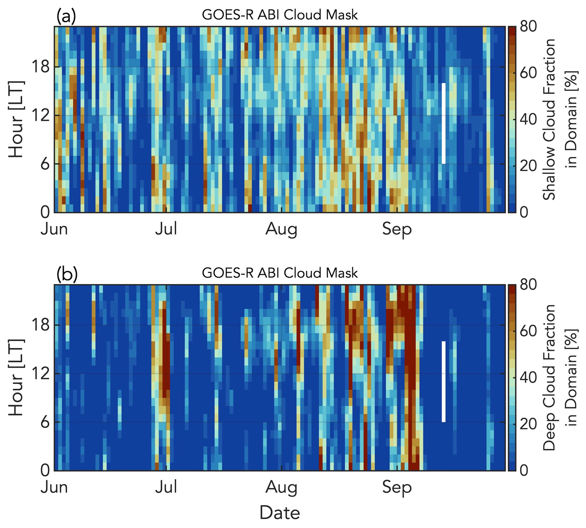
Figure 5 From 1 June–30 September 2022, the daily diurnal cycle in the Houston domain of (a) median shallow cloud fraction and (b) median deep cloud fraction. White spaces indicate missing data.

The diurnal variability in the domain-averaged shallow and deep precipitation is estimated as well (Fig. 6). The maximum hourly median shallow precipitation fraction in the dataset is 9.3 % at 15:00 LT on 15 July; meanwhile, the maximum hourly median deep precipitation fraction in the dataset is 63.7 % at 17:00 LT on 3 September. Of the 110 d that are not missing data and that have hourly median shallow precipitation fractions above 0 % all day, 19 have their maximum hourly median shallow precipitation fraction occur between 00:00 and 05:00 LT, 36 have their maximum occur between 06:00 and 11:00 LT, 42 have their maximum occur between 12:00 and 17:00 LT, and 13 have their maximum occur between 18:00 and 23:00 LT. Similarly, of the 95 d that are not missing data and that have hourly median deep precipitation fractions above 0 % all day, 9 have their maximum hourly median shallow precipitation fraction occur between 00:00 and 05:00 LT, 16 have their maximum occur between 06:00 and 11:00 LT, 54 have their maximum occur between 12:00 and 17:00 LT, and 16 have their maximum occur between 18:00 and 23:00 LT. Of the four variables thus far, the maximum hourly median deep precipitation fraction shows the strongest preference for a period of the day (12:00–17:00 LT), and the maximum hourly median shallow precipitation fraction occurs most frequently then, too. Overall, the precipitation activity is less widespread than the cloud activity. For 68 d (more than half of the total days), the maximum hourly median shallow precipitation fraction never exceeds 5 %, which includes 27 d in June, 26 d in July, 11 d in August, and 4 d in September. Similarly, for 81 d (two-thirds of the total days), the maximum hourly median deep precipitation fraction never exceeds 5 %, which includes 24 d in June, 23 d in July, 12 d in August, and 22 d in September. Finally, the deep precipitation in general is far more widespread than the shallow precipitation, as only 7 d have maximum hourly median shallow precipitation fractions greater than 5 %, while 23 and 10 d have maximum hourly median deep precipitation fractions greater than 10 % and 25 %, respectively.

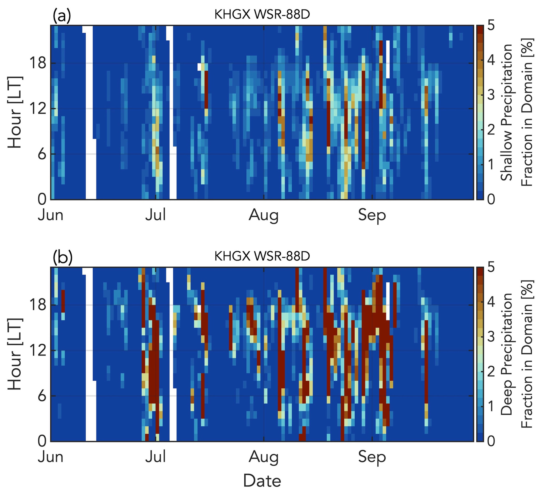
Figure 6 From 1 June–30 September 2022, the daily diurnal cycle in the Houston domain of (a) median shallow precipitation fraction and (b) median deep precipitation fraction. White spaces indicate missing data.

4.2 Shallow cloud fraction variability

Due to the high variability seen in Fig. 5a, a k-means clustering approach (Lloyd, 1982) is applied to the our satellite-based shallow cloud data to identify the dominant diurnal modes of shallow cloudiness across the analysis domain. A principal component analysis (Pearson, 1901) of the same data indicated that the first four principal components (or modes) account for over 90 % of the variability in the data. As a result, k is set to 4 in the k-means algorithm (Throndike, 1953), and we use the 121 median diurnal patterns of shallow cloud fraction as the input. Each day (13 September is not classified because of missing data) is assigned to one of four clusters. Finally, for each cluster, we identify the applicable days and calculate the median shallow cloud fraction and the shallow cloud fraction interquartile range every hour to create composite behaviors.

The diurnal variability in the four dominant modes of median shallow cloudiness and their interquartile ranges every hour for each of the four clusters are shown in Fig. 7. The four modes have distinct characteristics in terms of magnitude, shape, and timing of maxima and minima. Cluster 1 (C1) is the largest with 48 d grouped in this mode. C1 represents days with the lowest amount of shallow cloudiness, with the median shallow cloud fraction never exceeding 10 % (Fig. 7a). The median fraction is at its minimum at 23:00 LT; it then begins to grow at 04:00 LT and reach its maximum by 15:00 LT in the afternoon. The 21 d belonging to Cluster 2 (C2) have higher shallow cloud fractions and exhibit the opposite diurnal cycle compared to C1 (Fig. 7b). In C2, the median shallow cloud fraction is at its highest value at 22:00 LT while reaching its absolute minimum at 16:00 LT. In the 22 d comprising Cluster 3 (C3), the diurnal absolute maximum occurs at 02:00 LT, and the median shallow cloud fraction decreases steadily for the rest of the day (Fig. 7c). Finally, the 30 d in Cluster 4 (C4) are similar to C1 in that they both experience growth starting in the morning and continuing into the afternoon, but the growth rate is much steeper in C4. The shallow cloud fraction then becomes steady from the late afternoon onwards, which does not occur in C1. The median shallow cloud fraction reaches its maximum at 13:00 LT and then persists around that value for the rest of the day. Monthly calendars corresponding to the 4 months of the period and the cluster each day belongs to are shown in Appendix B.

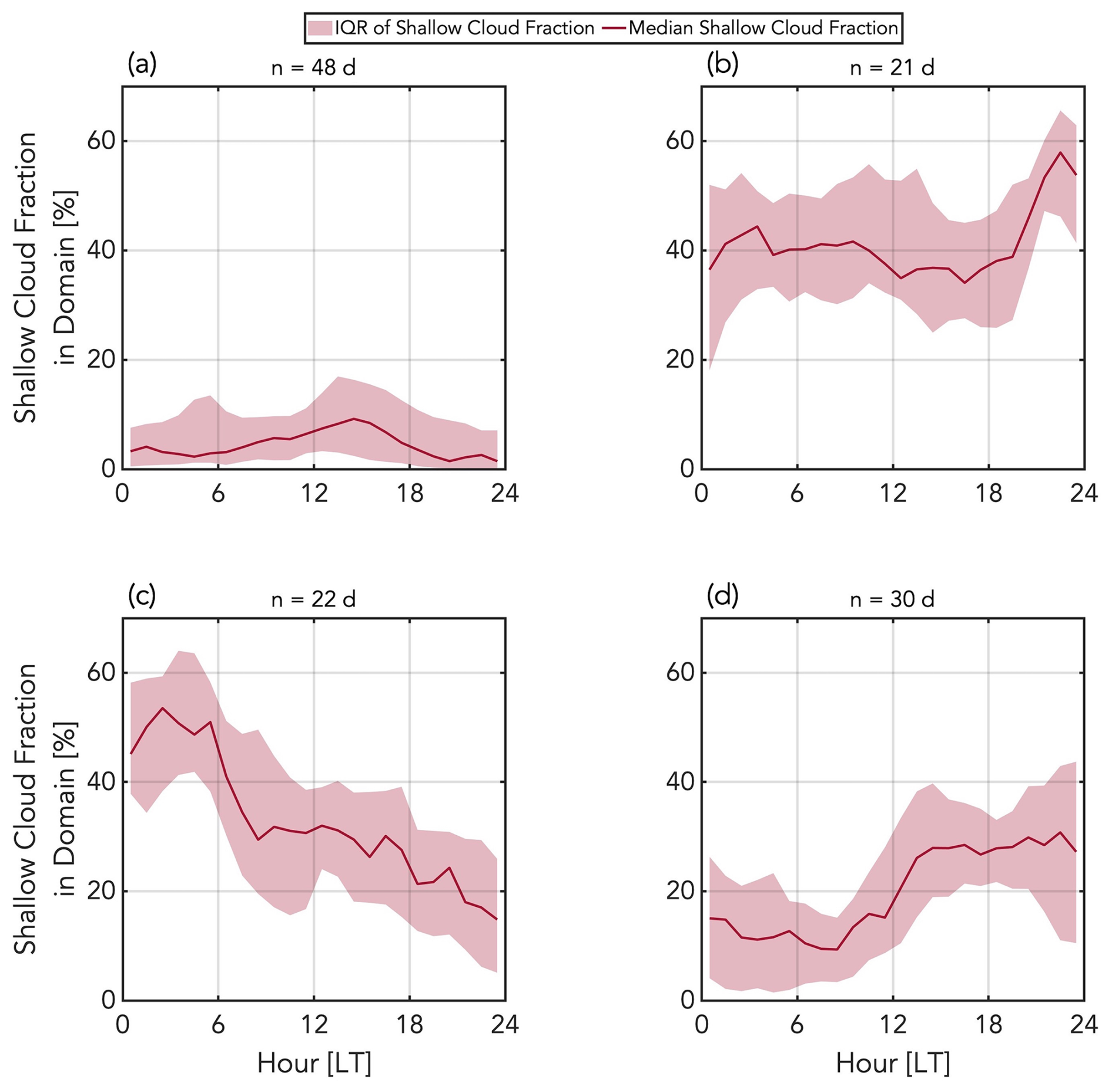
Figure 7 From 1 June–30 September 2022, the four modes of diurnal shallow cloud fraction in the Houston domain using k-means clustering. A total of 48 d belongs in Cluster 1 (a), 21 d in Cluster 2 (b), 22 d in Cluster 3 (c), and 30 d in Cluster 4 (d). Lines indicate the hourly median, and shading indicates the hourly interquartile range (IQR).

4.3 Cloud and precipitation fraction variability

The diurnal variability in shallow cloudiness and associated precipitation is affected by deep convective clouds, their mesoscale organization, and their impact on boundary layer organization. Using C1–4, the diurnal analysis is expanded to include the shallow precipitation fraction and the deep cloud and precipitation fractions. Their median hourly values, as well as the interquartile ranges, for C1–4 are shown in Fig. 8. C2 and C3 have significantly more fractional coverage of clouds with cold tops, and the median deep cloud fraction is above 0 % all day (Fig. 8b and c). Furthermore, the deep cloud fraction is higher than the shallow cloud fraction between 14:00 and 19:00 LT in C2 and between 15:00 and 18:00 LT in C3. In all clusters (Fig. 8a–d), the hourly median deep cloud fraction consistently reaches its diurnal maximum in the late afternoon. The timing of the shallow and deep cloud maxima differs, however: the maximum hourly median shallow cloud fraction occurs 6 h after the maximum hourly median deep cloud fraction in C2, while the maximum hourly median shallow cloud fraction occurs 14 h earlier than the maximum hourly median deep cloud fraction in C3 (Fig. 8b and c). Meanwhile, the shallow cloud fraction in C1 and C4 begins to increase in the late morning, and then the deep cloud fraction begins to increase 2–3 h later (Fig. 8a–d).

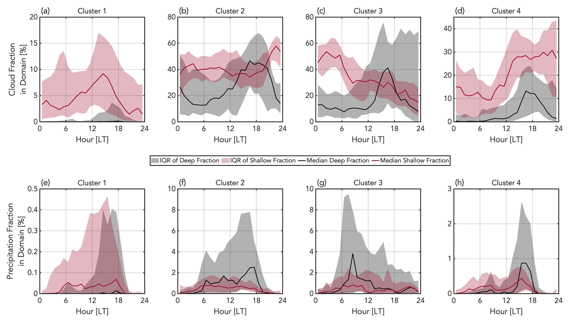
Figure 8 The diurnal shallow (red) and deep (black) cloud (a–d) and precipitation (e–h) fractions in the Houston domain corresponding to the four k-means clusters of diurnal shallow cloud fraction. Lines indicate the hourly median, and shading indicates the hourly interquartile range.

The domain is covered by far less precipitation, as noted before; the median shallow and deep precipitation fractions never exceed 5 % regardless of the cluster (Fig. 8e–h). Comparing the cloud and precipitation data, the median deep precipitation fractions in C1, C2, and C4, like the median deep cloud fractions, attain their diurnal maxima in the late afternoon. Meanwhile, in C3, the median deep precipitation fraction reaches its maximum earlier in the day than the median deep cloud fraction does. The median shallow cloud and precipitation fractions in all four clusters do not behave similarly and therefore have different timings of maxima. Lastly, like the deep cloud fractions, C2 and C3 have periods when the median deep precipitation fraction exceeds the median shallow precipitation fraction (Fig. 8f–g). C4 also has this feature in the precipitation data (Fig. 8h).

4.4 Land versus ocean

About 40 % and 60 % of the analysis domain is covered by ocean and land, respectively. Due to the prominent sea and land breeze circulations in Houston (Kocen, 2013) and the differences in convective properties over ocean and land, we repeat the analysis for the land and ocean portions of the analysis domain (Figs. 9 and 10). There are some noticeable differences in the timing and magnitude of the median shallow cloud fraction over land and over water. C1 shows a larger maximum median shallow cloud fraction occurring over water 5 h earlier than the one occurring over land (Fig. 9a and e), and, while both profiles see their largest values in the latter half of the day, the median shallow cloud fraction over land in C4 reaches its maximum before the median shallow cloud fraction over water does (Fig. 9d and h). Although the timing of the maxima in the shallow cloud fractions over land and over ocean is relatively similar in C2 and C3 (Fig. 9b, c, f, and g), the magnitudes over water are greater, meaning, across all four clusters, the median shallow cloud fraction over water is consistently greater than it is over land. On the other hand, we see that the maxima of the median deep cloud fractions over land and over water are similar in timing (a 1 h difference in C2, a 2 h difference in C3, and no difference in C4), but the magnitudes over land are higher than they are over water across all four clusters (Fig. 9). Breaking down the two surface types also allows us to see that the periods where the deep cloud fractions exceed the shallow cloud fractions in C2 and C3 from Fig. 8 persist regardless of land or ocean (Fig. 9b, c, f, and g).

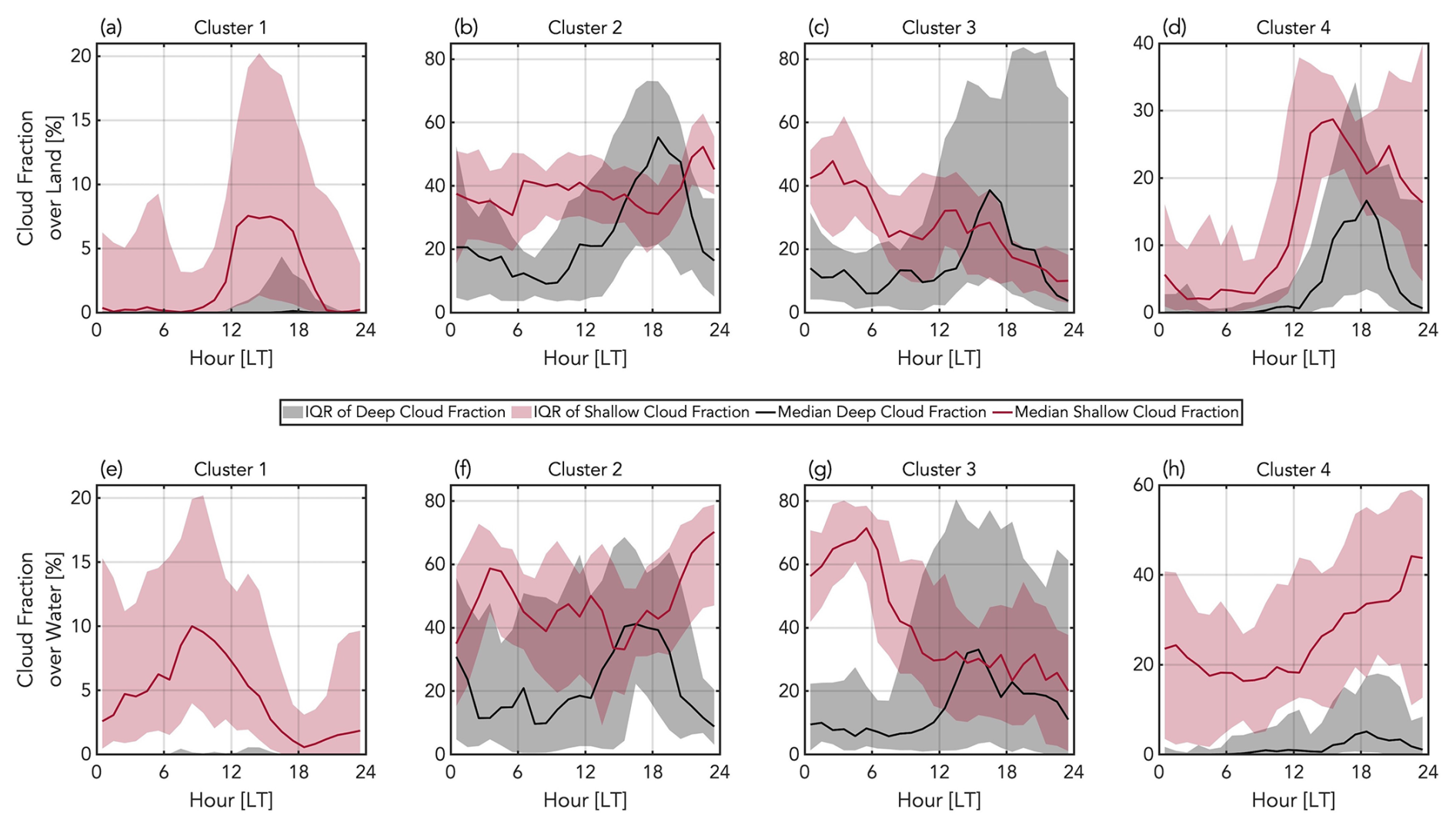
Figure 9 The diurnal shallow (red) and deep (black) cloud fractions over land (a–d) and over water (e–h) corresponding to the four k-means clusters of domain-wide diurnal shallow cloud fraction. Lines indicate the hourly median, and shading indicates the hourly interquartile range.

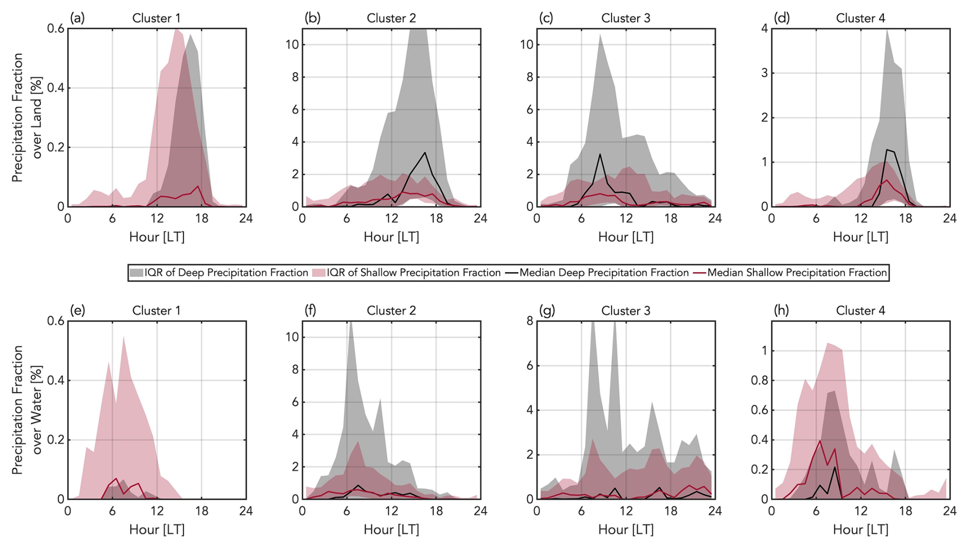
Figure 10 The diurnal shallow (red) and deep (black) precipitation fractions over land (a–d) and over water (e–h) corresponding to the four k-means clusters of domain-wide diurnal shallow cloud fraction. Lines indicate the hourly median, and shading indicates the hourly interquartile range.

Precipitation fractions behave differently according to surface types. The median deep precipitation fraction over water reaches its diurnal maximum before the median deep precipitation fraction over land does in C2 and C4 (Fig. 10), and the same goes for the shallow precipitation fractions in C1, C2, and C4. On the other hand, C3 indicates that the median deep and shallow precipitation fractions over land peak before they do over water (Fig. 10c and g). However, regardless of cluster, the maximum median deep and shallow precipitation fractions over land are higher than those over water. Also, the shallow and deep precipitation over land has a shift in timing depending on the clusters: the median shallow precipitation fraction peaks 2 h before the median deep precipitation fraction in C2 (Fig. 10b), at the same time in C3 (Fig. 10c), and at the same time in C4 (Fig. 10d). Comparing the cloud and precipitation data over land and over water, there is a larger discrepancy in the timing of the maximum deep precipitation and cloud fractions over land in C3 (Figs. 9c and 10c) than there is in C2 and C4. Lastly, C1's median deep precipitation fraction over land never exceeds 0 %.

We also calculate the diurnal cycle of the percentage of clouds and precipitation that are classified as shallow over land and over water in Clusters 1 and 4 in Fig. 11. Over land in C1, between 40 % and 65 % of clouds are shallow, with the minimum occurring at 08:00 LT and the maximum occurring at 13:00 LT, and between 20 % and 55 % of precipitation is shallow, with the minimum occurring at 19:00 LT and the maximum occurring at 06:00 LT (Fig. 11a). Over water in C1, the percentage of clouds that are shallow is similarly between 40 % and 65 %, but the minimum's and maximum's timings are reversed at 18:00 and 09:00 LT, respectively (Fig. 11c). The percentage of precipitation that is shallow shows far more variability over water than it does over land. Over land in C4, the percentage of clouds that are shallow is consistently higher than it is in C1, as 20 different hours feature a percentage greater than 60 % in C4 compared to 5 different hours in C1 (Fig. 11a and b). The cloud and precipitation percentages in C4 over land also have a similar diurnal pattern: a maximum attained in the morning hours between 08:00 and 11:00 LT followed by a steady decrease until the absolute minimum is reached after 16:00 LT (Fig. 11b). The precipitation percentage is also more variable over water than it is over land in C4 (Fig. 11d). Finally, a striking difference between land and water in C4 appears. The percentage of clouds that are shallow over water is steadily between 70 % and 85 %, and as noted already, the percentage of clouds that are shallow over land features a large decrease between morning and late afternoon. More exactly, the percentage for clouds over land starts at 84.4 % at 11:00 LT and reaches 50 % by 18:00 LT; meanwhile, in that same time frame, the percentage over water starts at 77.4 % and ends at 76.7 %.

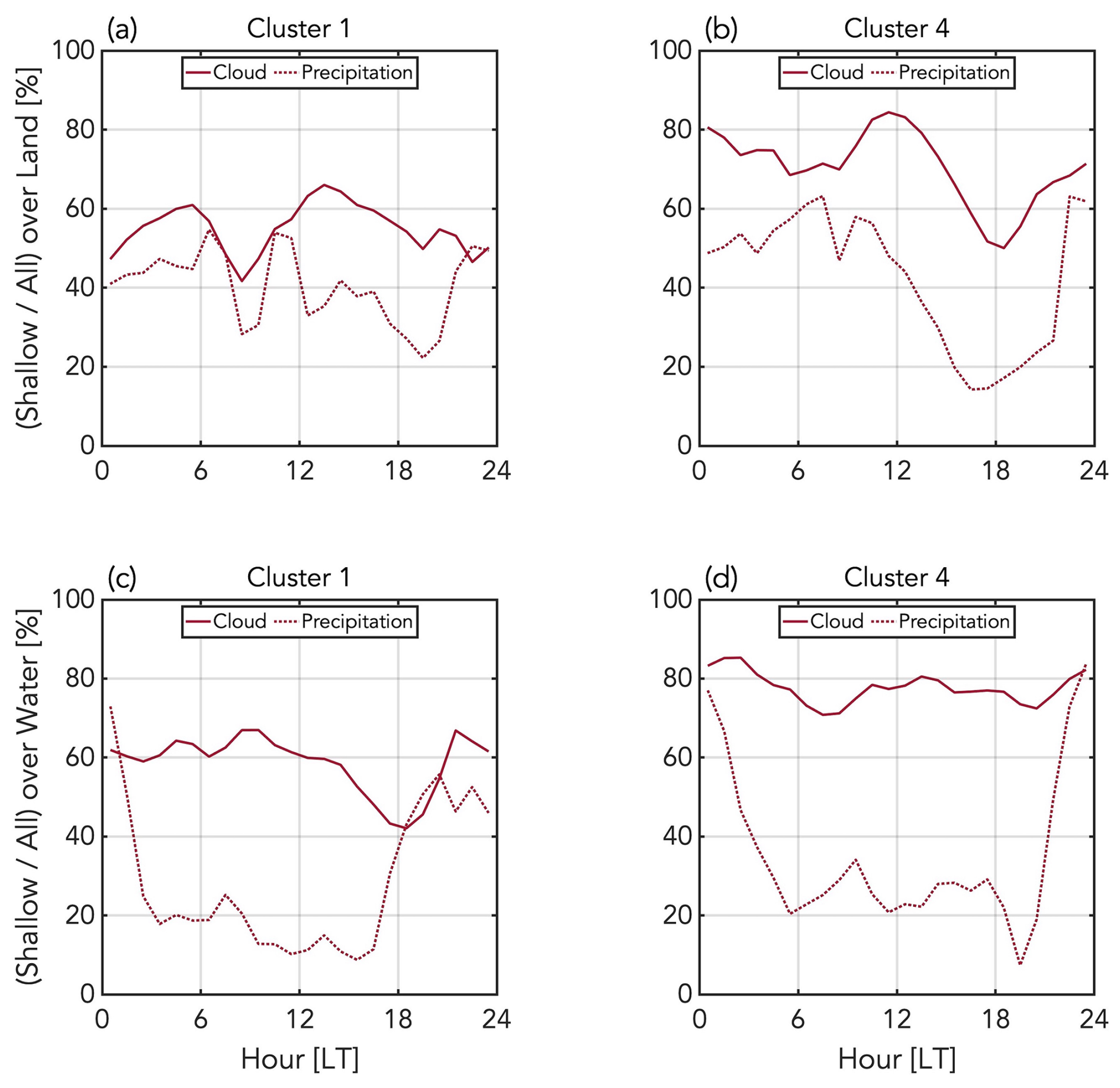
Figure 11 The diurnal cycle of the percentage of clouds (solid) and precipitation (dashed) classified as shallow over land (a, b) and over water (c, d) in Clusters 1 and 4.

4.5 Meteorological variability in the clusters

We use the meteorological observations provided by the soundings launched from the AMF1 site to establish our shallow versus deep classification in the radar data. The soundings and other instrumentation at the AMF1 site would be useful to quantify meteorological variability in the clusters, but point observations would limit our ability to look at variability across our large domain. So, we use HRRR model output, which has a high spatial resolution of 3 km, to provide this meteorological context as the best alternative to real observations. We compare the HRRR soundings at the grid point closest to the AMF1 site to the real soundings and find the median correlation coefficients for temperature, moisture, and wind speed to be high (>0.8; not shown). Even with this strong performance, we only qualitatively interpret the spatial patterns shown in the HRRR model data in our subsequent analysis.

We calculate composites of analysis at 850 hPa temperature, relative humidity, and wind speed and direction at 09:00, 13:00, and 17:00 LT for each of the four clusters in Fig. 12. There is a clear correlation between 850 hPa moisture and the deep cloud coverage in the cluster, as C1 and C4 feature the driest conditions at this level. The relative humidity minimum also shifts in C1 and C4 as the day progresses, starting in the northwestern part of the domain over land at 09:00 LT (Fig. 12a and d) and ending in the southwestern part of the domain over ocean at 17:00 LT (Fig. 12i and l). The opposite is true for the relative humidity maximum, which starts over the ocean in the morning and progresses over land by the late afternoon, located to the west of Houston–Galveston Bay (HGB) across all four clusters (Fig. 12i and l). The composite wind behavior across all four clusters is persistently weak onshore flow from the southeast in C1, C2, and C4 and the south and southwest in C3. The isotherms are oriented parallel to the coast all day in C1 and C4 to create a temperature gradient perpendicular to the coast, which, combined with the winds and moisture, favors sea breeze conditions. Despite a parallel-to-the-coast temperature gradient orientation at 09:00 LT in C2 and C3 (Fig. 12b and c), the gradient attains a more perpendicular-to-the-coast orientation later in the day, although it is not as pronounced as the ones shown in C1 and C4. Finally, C1 and C4 feature the highest temperatures, which shows a correlation between higher (lower) 850 hPa temperatures and more shallow (mix of shallow and deep) cloud activity.

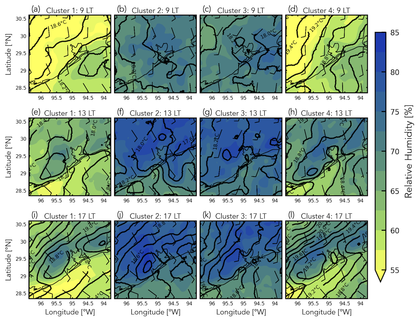
Figure 12 Composites of temperature (°C; black contours every 0.2 °C), wind speed and direction (knots; black barbs), and relative humidity (%; color shading) at 850 hPa for Clusters 1 (a, e, i), 2 (b, f, j), 3 (c, g, k), and 4 (d, h, l) at 09:00 LT (a–d), 13:00 LT (e–h), and 17:00 LT (i–l).

4.6 Spatial variability in Clusters 1 and 4

C1 and C4 are the most frequently occurring modes and represent atmospheric conditions with minimal to no deep clouds and precipitation. This provides an opportunity to examine the shallow clouds and precipitation present in these modes and to avoid potentially severe shallow cloud underestimation noted in the methodology, and so we will focus on these two clusters for the remainder of the study. The domain-averaged diurnal variability has indicated that the influence of the land–ocean contrast is important in determining the diurnal cycle. Here, the spatial variability in these two clusters during daytime (09:00–19:00 LT) is investigated. At every pixel, we calculate the number of shallow cloud occurrences and divide by the number of total data points. The spatiotemporal variability in shallow cloud frequency every 2 h from 09:00–19:00 LT for C1 and C4 is shown in Fig. 13. In the morning at 09:00 LT, shallow clouds in C1 are more frequently occurring over water, and a sharp gradient in shallow cloud frequency is observed across the coastline (Fig. 13a). The maximum in shallow cloud frequency (15 %–20 %) over the ocean during early morning hours is consistent with the diurnal variability in the oceanic shallow cloud fraction (Fig. 10e) that is at its maximum in the early morning hours and with the location of the 850 hPa relative humidity composite maximum (Fig. 12a). Later in the day, as a convective boundary layer forms over land, shallow cloud frequency begins to increase over land. The maximum of the C1 shallow cloud fraction is observed initially near the coast and gradually shifts further inland, following the 850 hPa relative humidity composite maximum. Aided by the onshore flow shown in Fig. 12, we hypothesize that the suppression of the shallow frequency near the coastline at this point of the day is due to the penetration of stable marine boundary layer air. In the meantime, shallow cloud frequency over the ocean gradually decreases and reaches a minimum after 17:00 LT (<5 %; Fig. 13e and f).

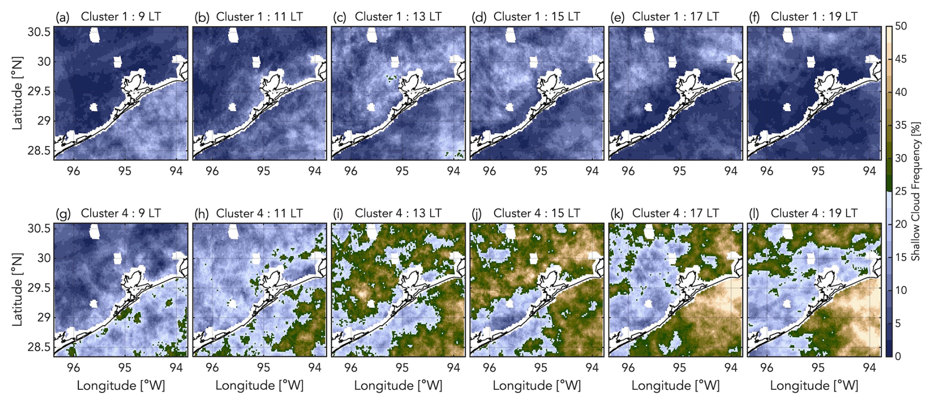
Figure 13 The frequency of shallow cloud occurrences at every pixel every 2 h from 09:00–19:00 LT for Cluster 1 days (a–f) and Cluster 4 days (g–l).

C4 is associated with much higher shallow cloud frequency (Fig. 13g–l). In the morning at 09:00 LT, higher shallow cloud frequency is observed over water than over land like in C1 (Fig. 13g), which corresponds to the 850 hPa relative humidity composite maximum like in C1, too (Fig. 12d). In the transition from late morning to early afternoon (Fig. 13h and i), the contrast in shallow cloud frequency between the ocean and land disappears, and shallow cumulus fields are observed across the domain with 25 %–35 % frequency. In C4, two noticeable spatial patterns are observed at 15:00 and 17:00 LT (Fig. 13j and k), and these patterns are not associated with the coastline and the surface type transition. First, over land, higher shallow cloud frequencies (25 %–40 %) are observed east of HGB, while, west of the HGB area, lower shallow cloud frequencies (10 %–25 %) are observed (Fig. 13j and k). Second, at 15:00 LT, the maximum shallow cloudiness is observed over land (Fig. 13j), and, at 17:00 LT as well as at 19:00 LT, the maximum shallow cloudiness frequency is observed over water, unlike in C1 (>40 %; Fig. 13k and l).

Overall, the spatiotemporal variability in the shallow cloud fractional coverage is significant. C1 represents more suppressed atmospheric conditions, and we hypothesize the land–ocean contrast and boundary layer stability likely explain most of the observed variability. C4 represents conditions that can support higher shallow cloud frequency. More complex processes and surface and atmospheric properties are responsible for the observed spatiotemporal patterns. The area east of the HGB is home to shipping lanes and most of the refineries and industrial complexes, while the area west of HGB has less polluted air (Kollias et al., 2024). No comprehensive aerosol data are available that can match the spatiotemporal sampling of the operational sensors used in this study; thus, no attempt is made to correlate the shallow convective clouds properties with aerosol conditions.

The corresponding spatiotemporal variability in shallow cloud top heights every 2 h from 09:00–19:00 LT for C1 and C4 is shown in Fig. 14. Using the soundings launched from the AMF1 site, we convert the T_B13 of the cloudy pixels to cloud top height, and we calculate the median cloud top height in 10 km × 10 km boxes (to enhance interpretability) every hour for each cluster. During early morning (09:00 LT), C1 shallow clouds have higher cloud tops (> 2 km) over land (Fig. 14a). During 11:00 and 13:00 LT, the cloud top heights over land are lower than they are over ocean (Fig. 14b-c). One noticeable feature is that higher cloud top heights are observed in the area east of HGB compared to the area west of HGB. This trend persists and amplifies as we progress through the day (Fig. 14d and e). On the other hand, C1 shallow cumulus over ocean have low cloud tops (< 1 km) and maintain these low cloud tops throughout the day. The higher cloud top heights east of HGB are also present in C4 (Fig. 14h–k). While shallow clouds get deeper west of the HGB in early and later afternoon (15:00–17:00 LT), the corresponding cloud top heights east of the HGB are higher (Fig. 14j and k). By 19:00 LT, the contrast between the sides of HGB muddies, and this is consistent in both clusters (Fig. 14f and l). The presence of shallow clouds with higher cloud top heights east of the HGB area is persistent and coherent in time and space while also being detectable in both C1 and C4. It suggests that, in this area, shallow clouds have stronger updrafts possibly driven by surface and aerosol properties.

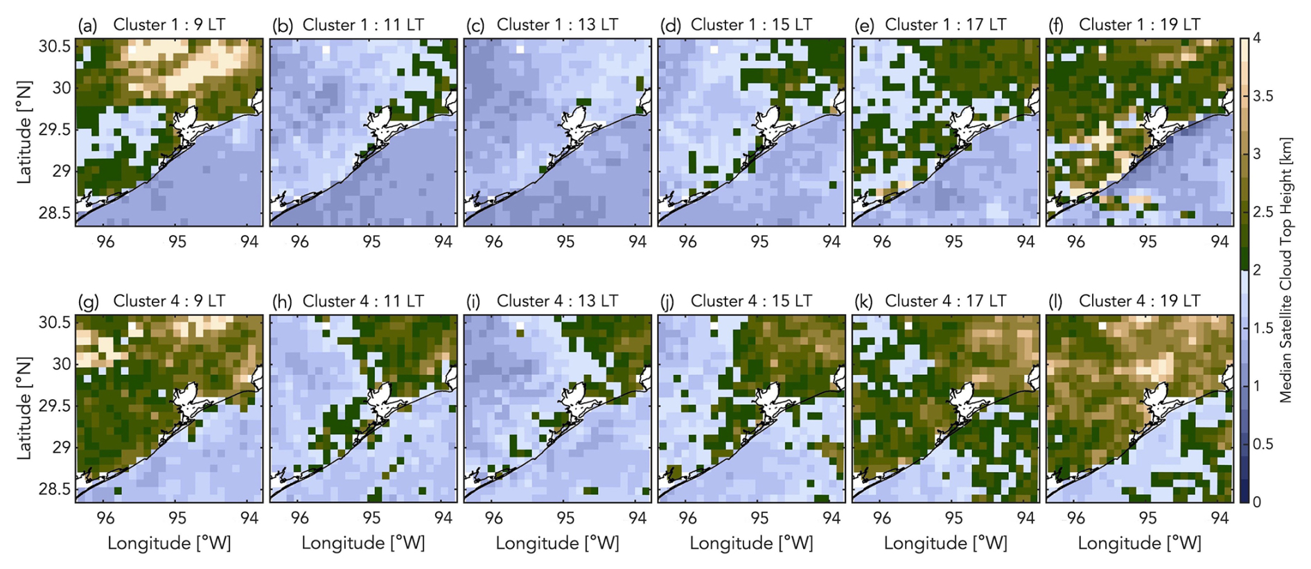
Figure 14 The median cloud top height of shallow clouds in each 10 km × 10 km box every 2 h from 09:00–19:00 LT for Cluster 1 days (a–f) and Cluster 4 days (g–l).

Finally, the combined KHGX and GOES-R cloud and precipitation data are used to estimate the spatiotemporal variability in the shallow-cloud-to-precipitation ratio for C1 and C4 in Fig. 15. For each 10 km × 10 km box, we divide the total number of shallow cloud occurrences (precipitating and nonprecipitating) by the total number of shallow precipitation occurrences every hour for each cluster. At 09:00 LT in C1, shallow clouds over ocean are more likely to precipitate than their counterparts over land, but, overall, the cloud-to-rain ratios are very low (Fig. 15a). A prominent band of very low cloud-to-precipitation ratios is observed at 15:00 LT on both sides of HGB (Fig. 15d), and the band of low cloud-to-precipitation ratios coincides with the area of high shallow cloud frequency in Fig. 13d. At 17:00 LT, a band with very high cloud-to-precipitation ratios is observed along the coastline, while a less pronounced band of low cloud-to-precipitation ratios is observed further inland (Fig. 15e). At 19:00 LT, little precipitation is observed in the domain (Fig. 15f). This signal is not observed in C4, as none of the six time periods examined have a pronounced area of low cloud-to-precipitation ratios.

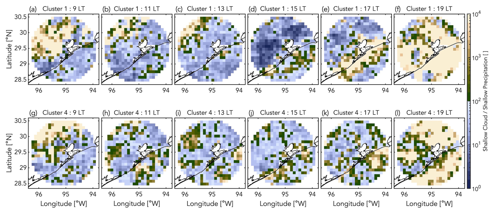
Figure 15 The ratio of shallow cloud occurrences to shallow precipitating cloud occurrences in each 10 km × 10 km box every 2 h from 09:00–19:00 LT for Cluster 1 days (a–f) and Cluster 4 days (g–l).

5 Summary and discussion

In this study, we characterize the spatiotemporal variability in clouds and precipitation properties in the Houston area during the ESCAPE and TRACER field campaigns. Operational satellite and radar datasets are used to provide large samples in time and space for statistics on cloud fraction, cloud top heights, and cloud-to-precipitation ratios over a 250 km × 250 km domain. A novel aspect of the proposed methodology is that we utilize the state-of-the-art instrumentation at the TRACER AMF1 to validate and constrain the operational datasets. We evaluate the performance of the GOES-R ACM and estimate a radar reflectivity threshold for KHGX that is applicable in the entire domain and can detect the light rainfall rate (< 0.1 mm h⁻¹).

Throughout the 4-month period, we identify shallow and deep clouds and associated precipitation, and we establish the four main diurnal patterns of shallow cloud fraction in the domain. We quantify the timing and magnitude of the cloud and precipitation occurrences while also noting the differences between land and water. Mainly, we find the cloud coverage is larger than the precipitation coverage, and we show that the deep clouds' coverage maximizes in the afternoon in all four modes, while three modes have deep cloud and precipitation coverages maximizing at the same time. Shallow cloud coverage is higher over water than it is over land, while the shallow precipitation coverage shows the opposite, and deep cloud and precipitation coverage is higher over land across all four modes.

One of the reasons for identifying the different modes of diurnal shallow cloud fraction variability is to identify time periods that have limited deep cloud activity. Clusters 1 and 4 fit this description and, at the same time, are the most populous clusters; thus, we have a robust sample size to study shallow clouds' spatiotemporal variability. Using this approach, we isolate regions and times of the day with interesting signals in shallow cloud frequency, shallow cloud top heights, and shallow precipitation fraction that warrant further consideration. For example, the presence of shallow clouds with higher cloud top heights east of the HGB is persistent and coherent in time and space. It suggests that, in this area, shallow clouds have stronger updrafts. We hypothesize that this could be due to aerosol properties given the large gradients shown in Kollias et al. (2024), in which we would need data on aerosol number concentration, composition, and supersaturation provided at different heights and high temporal resolutions to confirm a potential warm-phase invigoration signal. Given the onshore flow we showed, the clouds may be part of a synoptic-scale system over the Gulf of Mexico that is advected over land. The terrain itself may be higher in this region, which would cause stronger updrafts, too.

We also showed a prominent band of very low cloud-to-precipitation ratios in C1 in the early afternoon, and this band coincides with the area of maximum shallow cloud frequency. Later in the day, very high cloud-to-precipitation ratios are observed along the coastline, while lower cloud-to-rain ratios are observed further inland. Given the location and time of day of these signals, we hypothesize that the prominent sea breeze circulation in Houston (Kocen, 2013) is inducing shallow clouds to precipitate. The meteorological setup we showed in the HRRR composite maps suggests environmental conditions favorable for sea breeze formation, though to confirm the passage of sea breeze frontal boundaries over the AMF1 site, low-level thermodynamics would be needed. Other independent analyses show consistency with our findings, too. Most notably, Wang et al. (2024) used reanalysis to quantify the synoptic variability during the period and identified sea breeze circulations using surface meteorological data and operational datasets. Of the 46 sea breeze events they identified, 38 corresponded to days belonging in C1 and C4 (28 in C1 and 10 in C4). Over 70 % of their events fell into the anticyclonic regime defined in Wang et al. (2022), which corresponds to weak onshore flow and moisture advection that we also showed in our analysis.

Finally, this analysis will be useful and informative to the modeling studies in progress for ESCAPE and TRACER days, as their simulations can be benchmarked against our results. The correlations between the cloud and precipitation fields and the 850 hPa thermodynamics that we show could also inspire modeling studies that modulate the moisture and temperature gradients at different levels of the atmosphere and measure the cloud and precipitation response.

Appendix A

To provide a more comprehensive assessment of the cloud mask's skill, we use the following skill metrics:

$$\begin{array}{ll}{\displaystyle }& {\displaystyle }\text{accuracy}={\displaystyle \frac{\text{true positives (\#)}+\text{true negatives (\#)}}{\begin{array}{l}\text{true positives (\#)}+\text{false positives (\#)}\\ +\text{false positives (\#)}+\text{true negatives (\#)}\end{array}}},\\ {\displaystyle }& {\displaystyle }\text{precision}={\displaystyle \frac{\text{true positives (\#)}}{\text{true positives (\#)}+\text{false positives (\#)}}}.\end{array}$$

For our purposes, we use the ARSCL data as the truth and the cloud mask data at the grid point over the AMF1 as the prediction. We then consider a true positive to be an instance when both datasets report cloudy conditions, a false positive to be an instance when the cloud mask reports cloudy conditions and ARSCL reports clear conditions, a false negative to be an instance when the cloud mask reports clear conditions and ARSCL reports cloudy conditions, and a true negative to be an instance when both products report clear conditions.

One final consideration to make is the different temporal resolutions of the ARSCL and cloud mask datasets; the cloud mask provides data every 5 min and the ARSCL product provides data every few seconds. Initially, in the 5 min leading up to the cloud mask data point, if ARSCL has at least one cloud base height measurement, we designate the truth as cloudy and compare it to the prediction. The accuracy and precision of the cloud mask across the 4-month period are 75 % and 98 %, respectively, shown as the leftmost data points in Fig. A1a. The exceptional precision means the cloud mask is not false reporting cloudy conditions as clear conditions, but the accuracy leaves much to be desired. To improve the accuracy, we use stricter criteria: a greater fraction of the 5 min leading up to the cloud mask measurement must have cloud base height measurements in the ARSCL data. We incrementally increase this fraction until we reach 1 (or 100 %), meaning there must be cloud base height measurements for the entire 5 min period in the ARSCL data for the truth to be designated as cloudy. Figure A1a displays the accuracy and precision as a function of this percentage. At a value of 100 %, the precision drops to about 90 %, which is still satisfactorily high. The accuracy shows marked improvement, reaching 86 %. We use a percentage of 100 for the rest of the analysis.

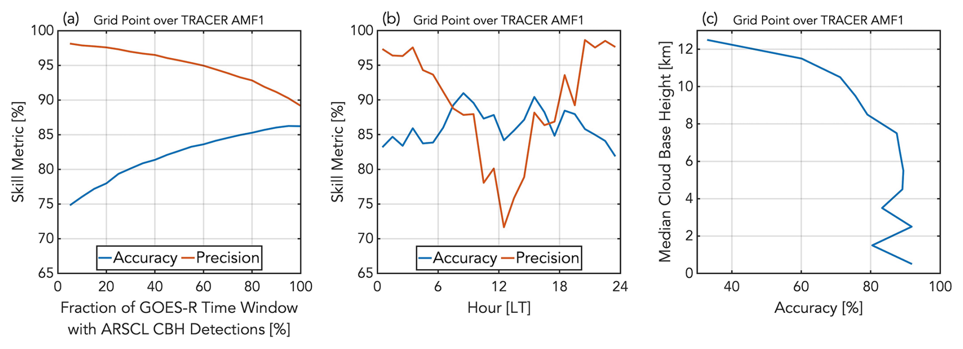
Figure A1 From 1 June–30 September 2022, using the cloud base height measurements from the TRACER AMF1 ARSCL product as the truth and the GOES-R ABI Cloud Mask values in the 0.5 km × 0.5 km grid point over the TRACER AMF1 as the prediction, the accuracy (blue) and precision (orange) of the GOES-R ABI Cloud Mask a function of (a) the percentage of the GOES-R time window containing ARSCL cloud base height detections in order for the “truth” to be designated as cloudy and (b) the local hour. (c) The accuracy of the GOES-R ABI Cloud Mask for increasing 1 km spaced bins of ARSCL median cloud base height during each 5 min GOES-R time window.

We calculate the accuracy and precision as a function of time in Fig. A1b during the 4 months. The accuracy stays between 81.9 % and 91 % throughout the day with an absolute maximum at 08:00 LT and a local maximum at 15:00 LT, and the precision is above 95 % between 00:00–03:00 LT (local maximum of 97.6 % at 03:00 LT) and 20:00–23:00 LT (absolute maximum of 98.6 % at 20:00 LT) while experiencing an absolute minimum of 71.7 % at 12:00 LT (Fig. A1b). Heidinger and Straka (2013), using CALIPSO measurements to validate the cloud mask, found a similar diurnal discrepancy, as they showed the cloud mask had a probability of detection (accuracy) of 93.9 % and a false cloud detection of 4.6 % over land during the day and a probability of detection (accuracy) of 89.5 % and false cloud percentage of 2.2 % over land at night. Jimenez (2020) compared the cloud mask to CALIPSO measurements over the contiguous United States and also found lower performance during the daytime in summer due to misdetections of clear-sky conditions. Both studies showed lower performance with low cloud as well, so lastly, we examine the accuracy as a function of cloud base height. We calculate the median cloud base height of each 5 min period and test the cloud mask's accuracy as a function of height. Figure A1c indicates the accuracy is greater than 80 % for median cloud bases less than 8 km; the accuracy decreases rapidly with median cloud base heights greater than this. These encouraging results suggests the cloud mask dataset is a feasible one for cloud research, and the improved performance for clouds closer to the surface in our analysis may be due to using ground-based measurements for validation instead of satellite-based measurements used in previous studies.

Appendix B

Monthly calendars corresponding to the 4 months of the ESCAPE and TRACER campaigns and the cluster to which each day belongs are shown in Fig. B1. June has a representative mix of the four clusters, with 12 C1 days, 5 C2 days, 6 C3 days, and 7 C4 days (Fig. B1), and July is similar, with 14 C1 days, 2 C2 days, 5 C3 days, and 10 C4 days. August and September shift the pattern, as August has the least C1 days (2 of 31 total days) of the 4 months, while C1 days dominate September (20 of 30 total days). To see the transition from consistent domain-wide shallow cloudiness in August to far less cloudiness in September leads us to believe we are observing the seasonal transition from summer to fall, which also marks the end of the convective season in Houston (Fridlind et al., 2019).

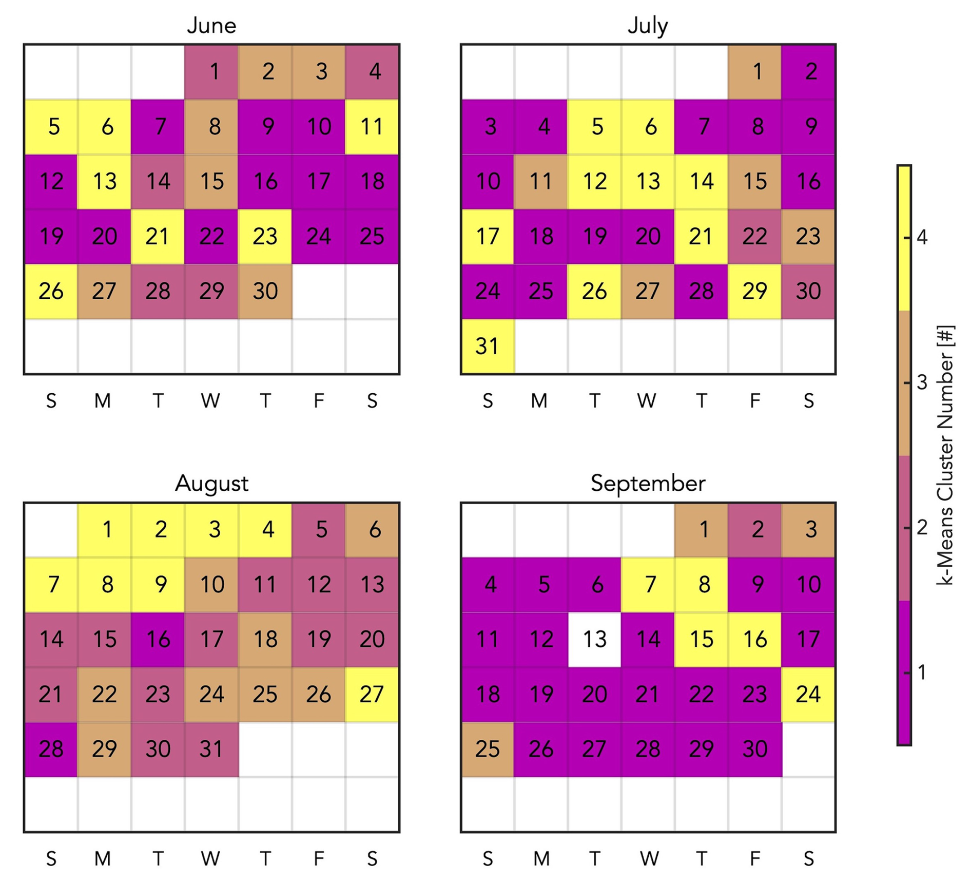
Figure B1 Monthly calendars for June–September 2022 denoting the four modes of diurnal shallow cloud fraction in the Houston domain that each day is classified as. The modes are determined using k-means clustering.