Influence of temperature and humidity on contrail formation regions in the general circulation model EMAC: a spring case study

While carbon dioxide emissions from aviation often dominate climate change discussions, non-CO₂ effects such as contrails and contrail cirrus must also be considered. Despite varying estimates of their radiative forcing, avoiding contrails is a reasonable strategy for reducing aviation’s climate effects. This study examines temperature and humidity, key atmospheric parameters for contrail formation, across different ECHAM/MESSy (European Centre Hamburg General Circulation Model/Modular Earth Submodel System) Atmospheric Chemistry (EMAC) model setups. EMAC, a general circulation model, is evaluated with various vertical resolutions and two nudging methods across seven specified dynamics setups. A higher vertical resolution aims to capture steep water vapour gradients near the tropopause, crucial for accurate contrail prediction. Comparisons with reanalysis data (March–April 2014) indicate a systematic cold bias (approximately 3–5 K in mid-latitudes), particularly in setups without mean temperature nudging. In the upper troposphere and lower stratosphere, all simulations exhibit a wet bias, while lower altitudes display a dry bias, both affecting contrail formation estimates. Point-by-point comparisons along aircraft trajectories confirm similar biases. Sensitivity experiments with varying thresholds of relative humidity over ice illustrate trade-offs between achieving high hit rates and minimising false alarms in contrail detection. A single-day case study integrating aircraft and satellite observations demonstrates that EMAC’s predicted contrail coverage aligns well with the observed formation. These results suggest that, despite existing temperature and humidity biases, EMAC generally captures regions favourable for contrail formation across diverse atmospheric conditions. Addressing model biases by refining temperature and humidity representation could significantly improve contrail prediction accuracy, strengthening contrail-avoidance strategies and supporting climate-optimised flight routing to mitigate aviation's overall climate effect.

1 Introduction

Estimates of the effective radiative forcing of aviation from 1940 to 2018 indicate that a significant part (best estimate two-thirds) stems from non-CO₂ effects, including contrails and NO_x and H₂O emissions (Lee et al., 2021). However, this estimated two-thirds contribution is a global and annual average, and especially the contribution from contrails varies significantly between individual flights (Grewe et al., 2014; Dahlmann et al., 2021; Teoh et al., 2022). Hence, operational mitigation options exist to avoid regions that are more climate sensitive than others. These regions are largely affected by the formation of strongly warming contrails or an over-proportional production of ozone from NO_x emissions. Methods are required to identify these climate-sensitive regions and enable their forecast within numerical weather prediction models. Originally, the ECHAM/MESSy (European Centre Hamburg General Circulation Model/Modular Earth Submodel System) Atmospheric Chemistry (EMAC) model was utilised to calculate climate change functions (CCFs) (Grewe et al., 2014; Frömming et al., 2021). More recently, Engberg et al. (2025) employed a comparable methodology using pycontrails 0.51.0, enabling direct comparisons between the two approaches as discussed in their study. These CCFs are a 4-dimensional measure of the global climate effect of individual local aviation emissions, depending on the location, altitude, and time of emission, as well as the prevailing meteorological conditions at the time of emission. By identifying regions particularly sensitive to aviation emissions, the CCFs represent the basis for climate-optimised, weather-dependent aircraft routing (Matthes et al., 2020; Lührs et al., 2018; Grewe et al., 2014). This study aims to provide additional information on model uncertainties relevant to the assessment of contrail climate effects. Additionally, the results from this study will serve as a basis for future recalculations of contrail-specific CCFs, further enhancing climate-optimised flight planning. As discussed by Grewe et al. (2017), the use of CCFs in daily operations requires the implementation of fast algorithms in daily weather forecast systems, and their corresponding mitigation potential must be evaluated in a consistent modelling framework. Such a framework ensures that the derived climate responses to aviation emissions are physically and methodologically coherent, allowing a fair comparison across different scenarios and emission types. Achieving this requires an integrated setup that includes the algorithmic CCFs as well as an air traffic optimiser integrated into a general circulation model. So far, this approach has only been applied to NO_x emission effects, and a validation exercise has been carried out to test the impact of NO_x emissions on ozone (Yin et al., 2023; Rao et al., 2022). Hence, we evaluate different EMAC model setups and analyse whether the model is able to reproduce basic meteorological fields from other models or observations. Since contrails have the largest effect on climate-sensitive regions and are therefore the primary target of air traffic management (Matthes et al., 2020; Lührs et al., 2021), we concentrate on the evaluation of contrail-forming parameters such as temperature and humidity in our study. These parameters are significant in identifying the regions where contrails may form and also influence their life cycle (Schumann, 1996; Kärcher, 2018). For instance, the use of particular temperature thresholds to calculate regions where contrails may form implies that significant differences between models and observations could lead to inaccurate forecasts of such regions and subsequently affect the climate-optimised aircraft trajectories, leading to an even greater climate response. Therefore, it is crucial that current climate models are evaluated to ensure their accuracy while at the same time being cautious of how model results are used further. The forecast of ice supersaturation in the atmosphere, which is a crucial factor for the formation of persistent contrails, remains a challenging area in aviation climate modelling (Gierens et al., 2020; Schumann et al., 2021; Rädel and Shine, 2010; Reutter et al., 2020; Tompkins et al., 2007). Climate models show different levels of humidity biases (Gierens et al., 1997; Brinkop et al., 2016; Kaufmann et al., 2018; Krüger et al., 2022). The EMAC model employed here exhibits a temperature bias in the upper-troposphere and lower-stratosphere (UTLS) region (Stenke et al., 2007; Jöckel et al., 2016), likely due to numerical diffusion of water vapour across the tropopause (Stenke et al., 2007), a known issue in climate models (Charlesworth et al., 2023). Nevertheless, because of the complex coupling between atmospheric dynamics and the hydrological cycle, other processes cannot be completely ruled out. In the setups considered here, we nudge temperature rather than humidity. Temperature is more stable and less variable in time and space, making it more suitable for spectral nudging towards reanalysis data at synoptic scales. In contrast, the higher spatial and temporal variability in water vapour makes direct humidity nudging both infeasible and potentially destabilising. Furthermore, no systematic analyses of the influence of model resolution or temperature nudging in “specified dynamics” setups on contrail prediction exist yet. To address this gap, we first compare key atmospheric parameters for contrail formation and life cycle across different EMAC model setups, placing special emphasis on comparing different methodologies of Newtonian relaxation (nudging) towards reanalysis data (specified dynamics setups). Second, we validate the model's ability to correctly identify regions where contrails are likely to form. We compare EMAC simulation results with atmospheric measurements by analysing temperature and humidity data sampled along the trajectories of the High Altitude and Long Range Research Aircraft (HALO) during the ML-CIRRUS (Midlatitude Cirrus) campaign. This comparison aims to assess how accurately the model reproduces observed conditions encountered in real flight scenarios. Finally, we evaluate satellite images and compare them with model-predicted contrail-forming areas obtained from our specified dynamics simulation. This paper is structured as follows: Sect. 2 describes the EMAC model and the experimental design (Sect. 2.1), followed by a description of the different methods to identify atmospheric conditions for contrail formation (Sect. 2.2). Afterwards, ECMWF reanalysis data (Sect. 2.3) and atmospheric observations used for the comparison (Sect. 2.4) are explained in detail. Section 3 compares temperature and humidity data calculated with different EMAC setups with ECMWF data while investigating the prediction of contrail formation areas. In Sect. 4, we compare contrail formation parameters along aircraft trajectories to highlight the discrepancy between simulated and observed quantities. Section 5 presents a more detailed analysis along the trajectory for a selected case study, accompanied by satellite images, and Sect. 6 discusses our principal findings. In Sect. 7, we summarise the key points, provide concluding remarks, and suggest aspects for future research.

2 Materials and methods

This subsection outlines the structure of the model and the corresponding simulations (Sect. 2.1) and explains the different methods to identify atmospheric conditions for the formation of persistent contrails (Sect. 2.2), followed by a brief summary of the reanalysis data used for the comparison (Sect. 2.3). In the final subsection, all sources of observational data are illustrated in detail (Sect. 2.4).

2.1 Atmospheric modelling: the Earth system model EMAC

Within the framework of the second version of the Modular Earth Submodel System (MESSy2), the EMAC model is utilised to investigate physical processes that are important for the climate effect of contrails. EMAC is a numerical chemistry–climate model simulation system that includes sub-models describing atmospheric processes from the troposphere to the mesosphere and their interactions with the ocean, land, and human influences. The fifth generation of the European Centre Hamburg General Circulation Model (ECHAM5; Roeckner et al., 2006) is used as the core atmospheric model. The physical subroutines of the original ECHAM code have been modularised and re-implemented as MESSy sub-models with ongoing development. ECHAM now only retains the spectral transform dynamical core, the flux-form semi-Lagrangian large-scale advection scheme (Lin and Rood, 1996), and the Newtonian relaxation-based nudging routines for specified dynamics model setups (Jöckel et al., 2010; Jöckel et al., 2016).

Experiment design and simulation setup

For the present study we applied EMAC (MESSy version 2.55) in a general circulation model setup (i.e. without interactive chemistry) with spherical truncation of T42 and T63 (corresponding to quadratic Gaussian grids of approximately 2.8 by 2.8° and 1.9 by 1.9° in latitude and longitude, respectively). We performed simulations with three different vertical resolutions, one with 31 (L31) vertical hybrid pressure layers, another with 41 (L41) vertical hybrid pressure layers, and a third one with 90 (L90) vertical hybrid pressure layers, reaching from the surface up to 10 hPa (L31), 5 hPa (L41), and 0.01 hPa (L90). The vertical resolution of the 41 layer simulation, similar to that with 90 layers, includes layers of about 20 hPa height in the UTLS region (see Fig. 1). While the L31 setup has the fewest vertical layers, it also has the lowest vertical resolution in the UTLS region. Within the L90 setup, there are more layers in the upper stratosphere above 50 hPa compared to the other setups. Due to the absence of these additional layers in the L41 or L31 model setups, various middle- and upper-stratospheric processes remain poorly represented. Consequently, the upper-stratosphere dynamics, such as the Quasi-Biennial Oscillation, are not accurately represented in L41 and L31. All simulations in this study obtained initial data (monthly averages of January 2013) on humidity and methane from the same L90 pre-simulation RD1SD-base-01. This is an EMAC-specified dynamics simulation that followed the reference D1 protocol of the Chemistry–Climate Model Initiative 2 (CCMI-2) (Plummer et al., 2021). The simulations were set up with Newtonian relaxation (nudging) towards the ERA5 reanalysis data (Hersbach et al., 2020). Additionally, a simulation with the L41 resolution also underwent nudging towards ERA-Interim reanalysis data for comparison (Dee et al., 2011). The nudging of the ECHAM5 base model is applied in the spectral space for four prognostic variables, namely divergence, vorticity, temperature, and the logarithm of the surface pressure. The corresponding relaxation times for nudging, defined as the time for a model variable to adjust to prescribed data, are 24 h for temperature and the logarithm of the surface pressure, 6 h for vorticity, and 48 h for divergence. The nudging strength is not applied homogeneously in the vertical dimension: the boundary layer and the layers above 126 hPa (L31), 100 hPa (L41), and 97 hPa (L90) are not nudged, and a transition zone with intermediate strength exists in between (see also Jöckel et al., 2016; Supplement). Two different nudging settings were used: in two cases, the global mean temperature (“wave zero”) was included for the Newtonian relaxations (T42L31 MTN – mean temperature nudging – and T42L41 MTN), and in all other cases it was omitted. A stronger interference in the case of the MTN simulations (involving additional nudging of global mean temperature at the designated model levels) results in a generally better agreement of EMAC model temperature with ERA5 reanalysis data. The differences and agreement between the model setups used are listed in Table 1. While no fully unnudged simulation was conducted for this study, previous work by Jöckel et al. (2016) has shown that the unnudged EMAC model exhibits both temperature and humidity biases. Standard nudging procedures (excluding global mean temperature nudging) already help reduce these biases compared to the completely free-running model state. Including the global mean temperature in the nudging (i.e. using MTN setups) further reduces the temperature bias and as a result also influences the humidity fields as shown in this study.

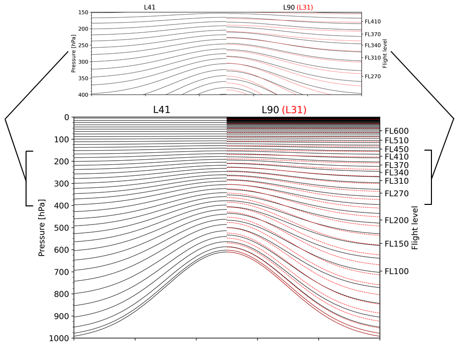
Figure 1 Vertical distribution of height levels in EMAC: L41 (left), L31 (right, red), and L90 (right, black) at a ground pressure of 1013 hPa and an idealised orography.

Table 1 Overview of the EMAC model setups used in this study. For the T42L41 STN setup, two simulations were performed with different nudging data (ERA5 and ERA-Interim, respectively), where STN refers to standard temperature nudging and MTN refers to mean temperature nudging.

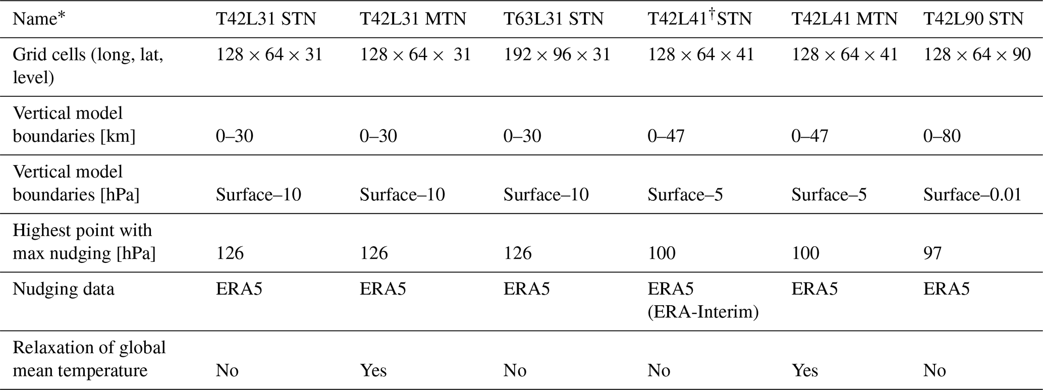
^* T refers to a triangular truncation at a specific wave number (42 or 63), corresponding to a quadratic Gaussian grid of approximately 2.8 by 2.8° and 1.9 by 1.9° in latitude and longitude, respectively, and L refers to the number of vertical hybrid pressure levels.

All simulations had a time step length of 10 min. As in RD1SD-base-01, the time evolution of the methane tracer at the lower model boundary was prescribed by Newtonian relaxation towards the data provided by CCMI-2. Since methane oxidation in the stratosphere constitutes a significant source of water vapour, accurately representing its variation is crucial for realistic atmospheric humidity distributions. In the CH₄ sub-model (Winterstein and Jöckel, 2021), the stratospheric water vapour contribution from methane oxidation is calculated using photolysis rates provided online by the photo-chemistry sub-model JVAL (Riede et al., 2009). This ensures that the background humidity conditions, which influence contrail formation and persistence, are more accurately represented. Two EMAC sub-models are particularly relevant to this study: S4D (“sampling in 4 dimensions”; Jöckel et al., 2010) and CONTRAIL (Version 1.0; Grewe et al., 2014). The CONTRAIL sub-model identifies regions where contrails and contrail cirrus may form and/or persist, as described in more detail in Sect. 2.2. The S4D sub-model enables online sampling of model data along aircraft flight trajectories. In previous studies, a standard bi-linear horizontal interpolation was used to determine the meteorological variables along these tracks. For this study, we adopt a newly implemented nearest-neighbour approach to capture local temperature and humidity conditions more accurately. Vertical interpolation, if needed, remains linear in pressure altitude in both cases. We utilised flight position files from the ML-CIRRUS campaign, which have a temporal resolution of 1 min. However, sampling occurs every model time step (10 min). After sampling, we separate the data into tropospheric (PV ≤2.5) and stratospheric (PV >2.5) regimes based on the model’s potential vorticity (PV). PV is a commonly used metric for distinguishing between the troposphere and stratosphere, as it provides a dynamic and physically meaningful representation of the tropopause, particularly in mid-latitude regions. The threshold value of PV = 2.5 PVU was selected according to Zängl and Wirth (2002). Based on the analysis, it is found that 55 % of the data points were in the troposphere, whereas 45 % were located in the stratosphere. Initially, a spin-up simulation was performed separately for each model setup from January 2013 to February 2014, producing output of global data, either instantaneous or temporal averages every 5 h. The main simulations were then performed from 1 March to 30 April 2014, with an output interval of 1 h. All analyses were conducted for the extended North Atlantic flight corridor (NAFC; 120° W–20° E), Asia (50–160° E), and the Northern Hemisphere between 80 and 20° N at pressure levels where air traffic takes place. The NAFC is of particular interest due to its high share of global air traffic and frequent occurrence of contrail formation conditions and because CCFs have been calculated in this region (Frömming et al., 2021).

2.2 Methods for identifying atmospheric conditions to form persistent contrails in global climate models

In this study, we investigate two different approaches to determine atmospheric regions capable of forming persistent contrails and contrail cirrus, without distinguishing between linear contrails and contrail cirrus. The first approach relies on fundamental contrail physics, providing a comprehensive representation of contrail formation and coverage, whereas the alternative method is more straightforward, enabling comparisons between EMAC and reanalysis data while focusing solely on ice supersaturation and contrail persistence. The more advanced method uses the parametrisations developed by Burkhardt et al. (2008) and Burkhardt and Kärcher (2009), as implemented in the EMAC CONTRAIL sub-model, to estimate the potential contrail coverage (PotCov). PotCov represents the fraction of a grid box that can be maximally covered by contrails under given large-scale temperature and humidity conditions. It is computed as the difference between (i) the maximum possible combined coverage of natural cirrus clouds and contrails and (ii) the coverage of natural cirrus clouds alone. Both coverage values depend on critical temperature and humidity thresholds with respect to ice, which are adapted for large-scale model conditions. These thresholds also incorporate the Schmidt–Appleman criterion (SAC; Schumann, 1996), which is derived from fundamental physical principles of mass, momentum, and energy conservation. In essence, the SAC determines whether hot exhaust gases mixing with cold ambient air will become supersaturated with respect to supercooled liquid water, enabling ice particle nucleation. This is often visualised using a “mixing line” in the temperature–humidity space, which tracks how temperature and humidity evolve as exhaust and ambient air combine. Besides ambient temperature and humidity, the SAC accounts for aircraft-related parameters such as propulsion efficiency and fuel combustion heat. In this study, we adopt engine parameters as provided by Grewe et al. (2014). Contrails persist only when the atmosphere is supersaturated with respect to ice; otherwise, they dissipate shortly after formation. Because these small-scale processes cannot be explicitly resolved in EMAC, their effects are represented through the parametrisations following Burkhardt et al. (2008). Further details on the calculation of PotCov are given in Grewe et al. (2014) and Frömming et al. (2021). Reanalysis data, such as ERA5, do not provide fields for PotCov directly. Therefore, an alternative approach is needed to compare the atmospheric potential for contrail persistence. This alternative identifies ice-supersaturated regions (ISSRs) following the methodology suggested by Dietmüller et al. (2023). ISSRs are usually defined by the following two criteria: the temperature must be below 235 K to separate it from mixed-phase regions (Pruppacher et al., 1998) and the relative humidity with respect to ice (RH_ice) must exceed 100 % (see Reutter et al., 2020). However, when studying the sub-grid-scale variability in the relative humidity field of numerical weather forecast model data, such as ERA5, it is essential to consider RH_ice thresholds below 100 % as demonstrated by Irvine et al. (2014). Dietmüller et al. (2023) explored different RH_ice thresholds for ERA5 and conducted a comparison with MOZAIC data (Petzold et al., 2020) in the European region. They found the best agreement between ERA5 and observations is achieved when the RH_ice threshold is set to 90 %. In this study we explore RH_ice thresholds between 90 % and 100 %. Here, we compare both approaches using identical EMAC atmospheric data under various model setups, as described in Sect. 3.2.

2.3 ECMWF reanalysis data

To assess simulation results fast and efficiently, a comparison with validated model results is useful. Reliable reanalysis data are required for an objective evaluation. Therefore, we utilised hourly and monthly global operational reanalysis data from the European Centre for Medium-Range Weather Forecasts (ECMWF) for March and April 2014. For our comparison, we used the fifth generation of ECMWF reanalysis (ERA5) data with a spatial resolution of approximately 31 km and 137 vertical hybrid levels reaching from the surface up to 0.01 hPa (about 80 km). At typical flight altitudes around 11.5 km (200 hPa), the vertical resolution is approximately 300 m (10 hPa). A comprehensive set of monthly mean temperature and specific humidity ERA5 data, which were aggregated from daily means, was provided by the German Climate Computing Center DKRZ on the high-performance computing system Levante. The data were re-mapped on a 0.25° × 0.25° grid and interpolated from the original ERA5 hybrid model levels to pressure levels. The same procedure was applied to the hourly data of temperature and specific humidity for 26 March 2014 (Hersbach et al., 2020). As there are no monthly or hourly relative humidity data available on Levante, we acquired these data from the Copernicus Climate Data Store. For temperatures above 273.15 K, the relative humidity is calculated based on saturation over water, while for temperatures below 250 K, it is calculated based on saturation over ice. For temperatures between 250 and 273.15 K, it is determined by interpolating between the values for ice and water using a quadratic function. The relative humidity data have 37 interpolated pressure levels and were re-gridded to a regular latitude–longitude grid of 0.25°. For our study, we only used relative humidity data between 200 and 350 hPa (Hersbach et al., 2023). All datasets have global coverage.

2.4 Atmospheric observations

Further knowledge on the performance of the model can be gained through comparing model data and observations. While a global coverage is normally not available for most atmospheric parameters at high resolution, comparing specific areas can provide valuable insight into the accuracy of model parameters and opportunities for model improvement. In this study, measurement data from the Midlatitude Cirrus (ML-CIRRUS; Voigt et al., 2017) measurement campaign are compared with EMAC model results at cruise altitude. Furthermore, satellite measurements were utilised to compare the areas where contrail formation was predicted in the model with observed contrails.

2.4.1 Aircraft experiment ML-CIRRUS

The ML-CIRRUS campaign, which took place from 10 March to 16 April 2014, was one of the first scientific missions to demonstrate the capabilities of the novel High Altitude and Long Range Research Aircraft (HALO; https://halo-research.de, last access: 2 June 2025). A comprehensive overview of the scientific objectives, flight plan, and equipment is provided by Voigt et al. (2017). Over the campaign period, HALO conducted 16 research flights, which amounted to a total of 88 flight hours. The flights were designed to comprehensively characterise mid-latitude cirrus and contrail cirrus using in situ and remote sensing instruments. Unlike young contrails, which can be distinguished from natural cirrus by their exceptionally high concentrations of very small ice crystals (diameters < 10 µm), aged contrails (i.e. contrail cirrus) become microphysically similar to natural cirrus (Krämer et al., 2020). Consequently, identifying contrail cirrus solely by their properties is challenging. For the ML-Cirrus study, contrail cirrus forecasts from the CoCiP model (Schumann, 2012) guided the flight planning process, allowing the targeted sampling of regions where contrail cirrus were likely to occur and enabling a comparative analysis of both cloud types. The ML-CIRRUS project aimed to enhance our understanding of cirrus cloud formation across varying meteorological conditions (Krämer et al., 2016; Luebke et al., 2016; Wernli et al., 2016; Urbanek et al., 2017), to refine our estimations of the radiative impact of cirrus (Krisna et al., 2018), and to assess air traffic impacts on high cloud cover (Schumann et al., 2017; Grewe et al., 2017; Li et al., 2023). The flights covered almost the entire central European region from the northern British coast to Portugal. To fulfil the scientific objectives of the mission, the HALO payload for ML-CIRRUS consisted of the instrumentation for measuring cloud particles, aerosols, and trace gases including five different water vapour instruments. For our research, we analysed data collected by a fast in situ stratospheric hygrometer (FISH). This closed-cell Lyman-α photofragment fluorescence hygrometer has been used on multiple research aircraft for over 2 decades (Meyer et al., 2015; Schiller et al., 2009). The instrument's operating principle is described in detail by Zöger et al. (1999). FISH is capable of measuring water vapour mixing ratios ranging from 1 to 1000 ppm. The overall uncertainty during ML-CIRRUS was found to be 6 % relative with a ±0.4 ppm absolute offset uncertainty (Kaufmann et al., 2018). It is important to note that FISH measures “total water”, which includes gas-phase water as well as evaporated ice crystals. When comparing with gas-phase H₂O from the model, only values up to 80 % RH_ice are used to exclude clouds, as within clouds, RH_ice is elevated due to ice particles. Therefore, we substituted all FISH values (with a water vapour mixing ratio > 15 ppmv) where RH_ice was larger than 80% with measurements from the SHARC (Sophisticated Hygrometer for Atmospheric ReseaRCh) sensor. SHARC is a tunable diode laser hygrometer and is part of the Basis HALO Measurement and Sensor System (BAHAMAS; Giez et al., 2023). This closed-cell hygrometer uses the absorption line of water vapour at 1.37 µm. More details about the configuration of the SHARC sensor during the ML-CIRRUS campaign can be found in Kaufmann et al. (2018). The temperature data used in this study were also measured by BAHAMAS (Giez et al., 2023). Since the interval of the observation data is 1 s, the alignment with the 10 min interval of the model is important. Initially, we computationally derived weighted average mean values for the measurement data through the implementation of a Gaussian filter. We utilised the fact that infinite repetitions of a boxcar filter can be converted into a Gaussian filter (Gans and Gill, 1984) and therefore performed multiple loops of a centred rolling mean to achieve a weighting of the data. Following this, the data were resampled to 10 min intervals. For spatial alignment, we used the averaged positions derived from the ML-CIRRUS flight track data as input to the EMAC sub-model S4D (Jöckel et al., 2010). The S4D sub-model interpolates the 3-dimensional model fields to the exact geographical location and time corresponding to each 10 min averaged observational data point. This procedure ensures that the model data are sampled at the correct geolocation, thereby minimising spatial representativeness errors. To focus on contrail formation regions and remove outliers, we restricted observed values to temperatures below 240 K, resulting in 308 data point pairs (51 h of flight time). We then computed the correlation between the observational and model data using a linear regression analysis.

2.4.2 Satellite data

The SEVIRI instrument on board the geostationary Meteosat Second Generation (MSG) satellite is used to observe contrails in the region probed by the HALO aircraft during ML-CIRRUS on 26 March 2014. This is the most prominent contrail outbreak encountered during the ML-CIRRUS campaign and has been investigated using in situ cloud probes, airborne lidar observations, and MSG–SEVIRI data in Wang et al. (2023). Thus, this day is very well suited for a comparison with the climate model data investigated in this study. These observations were conducted over the North Atlantic region, specifically near the coast of Ireland. This area is strategically significant as it lies along the major air traffic routes between Europe and the United States, making it a prime location for studying contrail formation and behaviour (Sect. 2.4.1; see also Wang et al., 2023, for a detailed evaluation of this flight). The SEVIRI imager (Schmetz et al., 2002) on board the operational MSG satellite MET-10 observes the Earth in 11 spectral channels with a spatial sampling distance of 3 km at the sub-satellite point and a temporal resolution of 15 min. Due to its location in the geostationary orbit above 0° E this sensor is well-suited to observe Europe. However, it has limitations, such as being unable to fully capture regions like the western North Atlantic Ocean. Additionally, the spatial resolution decreases towards the edge of the observed Earth disc, making it challenging to identify small structures like contrails. In this study, false colour composites (so-called ash RGBs) are used in order to visually spot contrails. These ash RGBs combine three brightness temperatures and temperature differences for the MSG–SEVIRI channels centred at 8.7, 10.8, and 12.0 µm. Here, contrails appear as dark blue or black linear objects and are easy to identify. This type of image is often used as a basis for automatic contrail detection as e.g. in Meijer et al. (2022). In this study, we restrict ourselves to a visual analysis of the ash RGBs in order to identify areas of frequent contrail formation. Furthermore, the use of purely thermal channels makes these observations independent of solar illumination such that the ash RGBs can be used during day and night. However, the moderate resolution of MSG–SEVIRI only allows contrails to be distinguished that are 30–60 min old (Vázquez-Navarro et al., 2015; Gierens and Vázquez-Navarro, 2018). These are persistent contrails which have formed in ice-supersaturated regions and can live for hours. For the sake of comparison with the model results, the data are remapped from the original satellite projection to an equal longitude–latitude grid.

3 Influence of different vertical model resolutions and nudging techniques on temperature, humidity, and ice supersaturation

As the representation of key meteorological parameters is critical for the understanding of contrail formation and life cycle, this sections identifies differences in the atmospheric distribution of temperature and humidity between EMAC simulations with various vertical (L31, L41, L90) and horizontal (spectral) resolutions (T42, T63) and different nudging approaches (standard temperature nudging (STN) or mean temperature nudging (MTN)). Firstly, the simulated temperature and humidity of various model setups are compared to ERA5 data in three specific regions (NAFC, Asia, and the whole Northern Hemisphere) for March and April 2014. In order to better understand the local peculiarities, the parameters were examined separately within 20° latitude bands for all selected regions. In the end, this analysis focuses on the temperature and humidity data for 26 March 2014. Here, two distinct methods are used to calculate potential contrail formation regions for this specific day.

3.1 Temperature and humidity profile comparison for March and April 2014

Figure 2 illustrates the area-weighted mean temperature across six distinct EMAC model setups (see Table 1) for the extended NAFC between 50 and 400 hPa in comparison with ERA5 for March and April 2014. Notably, our comparison reveals a cold bias in EMAC simulations with standard temperature nudging compared to ERA5 reanalysis data for the analysed region. The identified bias for the area-weighted average mean temperature data ranges from 3 to 5 K between 400 and 50 hPa, with the most significant discrepancy around 200 hPa. Increasing the spectral (horizontal) resolution from T42 to T63 leads to a minimal reduction in the bias, by up to 0.2 K, while changes in vertical resolution have a negligible effect. The STN model setup with 41 vertical layers exhibits the strongest deviation from ERA5, being 0.1 K colder than other STN setups up to 100 hPa. The analysis of 20° latitude bands for the NAFC (Fig. 4, left) indicates a consistent altitude-dependent temperature bias across all bands. However, the application of mean temperature nudging (T42L31MTN, T42L41MTN), as explained in Sect. 2.1, significantly reduces, as to be expected, the cold bias to less than 0.1 K across all analysed pressure levels and bands. Since the STN setups constrain only selected meteorological variables (e.g. vorticity, divergence, temperature, and surface pressure) to large-scale reanalysis patterns without enforcing an accurate global mean temperature, a systematic global temperature offset can still develop. In contrast, the MTN setup imposes an additional constraint on the global mean temperature, preventing such a systematic bias from emerging. As a result, MTN keeps the model closely aligned with the reanalysis, making the temperature bias almost negligible. In the MTN setup, the bias is only present above 80 hPa, a region where no nudging is applied. The impact of both nudging concepts on the temperature difference relative to ERA5 is also evident in the Asian region (see Figs. S1 and S11 in the Supplement) and across the entire Northern Hemisphere (see Figs. S2 and S12). Small differences can be found in the Asian region above 80 hPa, where simulations (except L90) exhibit a warm bias (up to 1 K), regardless of the applied nudging method. The analysis of relative humidity over ice in the extended NAFC during March–April 2014, presented in Fig. 3, reveals up to 30 % higher mean values at each EMAC grid point compared to ERA5 across four pressure levels (200, 250, 300, and 350 hPa). The MTN simulations, on average, exhibit closer agreement with ERA5 than the STN simulations, with noticeable differences across pressure levels. At 200 hPa, MTN simulations differ typically by 5 %–12 %, while STN ones differ typically by 12 %–17 %. At 250 and 300 hPa, differences between all STN model setups are further reduced, while the difference between EMAC and ERA5 remains consistent on average. Analysis shows that the vertical resolution does not play a central role, but increasing the spectral (horizontal) resolution to T63 diminishes the difference from ERA5 across all investigated pressure levels.

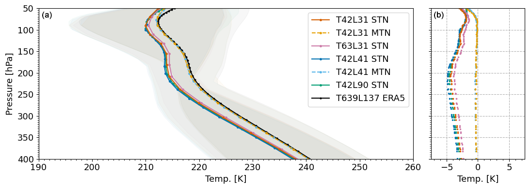
Figure 2 (a) Area-weighted mean temperature distribution from EMAC simulations with different vertical resolution (L31: red; L41: blue; L90: green) and ERA5 data (L137: black) for the North Atlantic flight corridor. The mean values for each grid box were calculated beforehand using hourly data spanning March to April 2014. Nudging approaches: standard (STN, solid) and mean (MTN, dashed) temperature nudging, with 95th percentiles shaded. (b) Temperature difference between EMAC and ERA5.

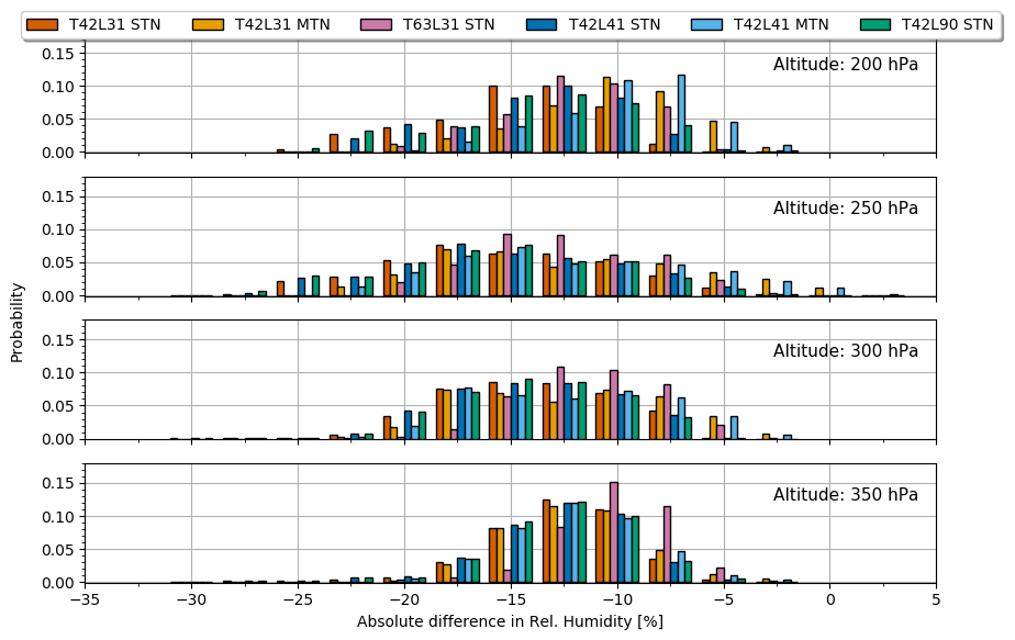
Figure 3 Probability density functions illustrating the absolute differences in relative humidity over ice (given in percentage points) between various EMAC model setups and ERA5 data (ERA5 minus EMAC) in the extended NAFC region for March and April 2014. The figure displays the distribution for four vertical pressure levels, starting from 200 hPa at the top and concluding with 350 hPa at the bottom. At each pressure level, the vertical model resolution and nudging method is indicated by different colours: red (L31), dark blue (L41), and green (L90) for standard temperature nudging and orange (L31) and light blue (L41) for mean temperature nudging. A dataset with higher horizontal resolution (T63) is represented in purple.

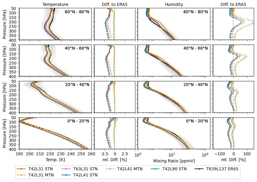
Figure 4 Temperature and humidity distribution from various EMAC simulations with different vertical resolution (L31: red; L41: blue; L90: green) and ERA5 data with 137 vertical levels (black) for the North Atlantic flight corridor. Nudging approaches: standard (STN, solid) and mean (MTN, dashed) temperature nudging. Left: area-weighted mean temperature distribution and difference from ERA5 for all EMAC setups. Right: area-weighted mean humidity mixing ratio distribution and difference from ERA5 for all EMAC setups. The mean values for each grid box were calculated beforehand using hourly data spanning March to April 2014. The 95 % percentile of each simulation is marked as grey shade.

The variation in distributions between simulations with mean and standard temperature nudging is smaller for the NAFC region than for the entire Northern Hemisphere. In the Northern Hemisphere (Fig. S7), a larger spread in the relative humidity over ice difference between EMAC and ERA5 can be observed for all analysed simulations and pressure levels, with certain EMAC grid points indicating lower relative humidity than ERA5. In the Asian region (Fig. S6), distributions at 250 and 300 hPa resemble those of the NAFC region and the Northern Hemisphere, while at 200 hPa substantial disparities from ERA5 are evident. When looking at probability density functions (PDFs) of the ERA5 and EMAC model setups separately (Figs. S15, S16, and S17), a shift toward higher humidity values in EMAC setups compared to ERA5 is noticeable at all pressure levels. The altitude-dependent cold bias can partly explain the disparity in relative humidity between ERA5 and EMAC in the STN simulations, as the saturation vapour pressure over ice depends solely on temperature (Eq. A3). However, an analysis of specific humidity values is necessary to understand discrepancies in simulations involving mean temperature nudging. Subsequently, we examined the vertical distribution of specific humidity along 20° latitude bands for the three selected areas. In the extended NAFC (Fig. 4), an altitude- and latitude-dependent humidity bias that differs from the nudging concept is apparent. For MTN simulations, a consistent wet bias is observed at higher altitudes (150 to 250 hPa), significantly differing from ERA5. While differences are minimal in the tropics, a substantial bias exists in the mid-latitudes (40 to 80°). This results in higher relative humidity over ice values for MTN simulations compared to ERA5 despite similar temperatures. In contrast, simulations driven by STN exhibit a dry bias below 250 hPa for all latitude bands compared to ERA5. Additionally, they display a wet bias north of 40° at heights between 150 and 250 hPa. The dry bias at lower levels (350 hPa) compensates for the slight temperature bias, yielding relative humidity over ice values closer to ERA5 when compared to other pressure levels (Fig. 3). At 300 hPa, STN simulations reveal a temperature bias increase, while the dry bias remains unchanged, resulting in a minimal rise in relative humidity over ice difference from ERA5. The temperature bias in STN simulations peaks at 250–200 hPa, accompanied by a wet bias intensifying at higher latitudes. However, the overall bias is reduced on average due to lower values at lower latitudes. No significant differences are observed between simulations with different vertical resolutions. In the other investigated regions, similar results are found. It is evident that a substantial bias in specific humidity exists in the MTN setup, particularly at higher altitudes and northern latitudes. Nevertheless, the effect on relative humidity weakens at higher altitudes because of the pressure-level-dependent vapour pressure. Higher relative humidity values have a direct impact on the prediction of ISSRs, as exceeding the threshold values more frequently leads to an overestimation of regions where contrails can persist. Similarly, the temperature bias affects contrail formation predictions; a systematic cold bias in the temperature data shifts the perceived temperature closer to or below the critical threshold in the SAC. This results in contrails being predicted in conditions where, in reality, the ambient temperature is warmer than the critical threshold and contrails would not actually form.

3.2 Contrail-forming areas in different model setups

Our numerical simulations utilising seven different model setups reveal differences in horizontal size (area) of regions where contrails could form (potential contrail cover) or persist. With both methods outlined in Sect. 2.2, we first analyse contrail coverage areas for thresholds at 90 %, 95 %, and 100 % RH_ice below 235 K at three distinct pressure levels (see Table 2) in a specific synoptic situation (26 March 2014, 12:00 UTC), where research aircraft observations from the ML-CIRRUS campaign are available (see Sect. 2.4.1). Reducing the humidity threshold from 100 % to 95 % and to 90 % results in an increase in contrail coverage areas by a factor of about 2 and 2.5, respectively. Due to the differences in temperature and humidity between the model and ERA5 reanalysis data, all EMAC setups generally exhibited a larger ice-supersaturated region compared to ERA5. Simulations with standard temperature nudging, irrespective of vertical resolution, indicate larger contrail coverage areas for each pressure level and RH_ice threshold. Transition to a T63 resolution yielded a marginal decrease in coverage of approximately 1 percentage point. At 250 hPa, MTN simulations display nearly identical covered areas as ERA5 for the 90 % (15 %–16 % coverage) and 95 % (11 %–13 % coverage) thresholds. In contrast, STN simulations show 10 % (> RH_ice 90 %) to 8 % (> RH_ice 95 %) more potential contrail formation areas at this pressure level. At 300 and 350 hPa, MTN simulations overestimate ERA5 results by 5 % to 7 %, while STN simulations overestimate by 7 %–16 %. However, for the 100 % threshold, EMAC MTN results agree with ERA5 at 300 hPa, while they underestimate at 250 hPa by 3 % and overestimate at 350 hPa by 3 %–4 %.

Table 2 Percentage of areas indicating contrail formation based on the ISSR and PotCov methods at various pressure levels, using different model setups over the NAFC on 26 March 2014 at 12:00 UTC. For the ISSR method, three relative humidity over ice (RH_ice) thresholds (90 %, 95 %, and 100 %) are used. Potential contrail cover (PotCov) areas are calculated directly in EMAC and are provided as total (PotCov > 0) and grid-box-adjusted coverage areas. The grid-box-adjusted coverage is determined by multiplying each grid box area by the potential contrail cover for that box and then dividing the area-weighted sum of all covered areas by the area-weighted sum of the entire area. The area-weighted mean PotCov is calculated over all grid boxes with PotCov above zero.

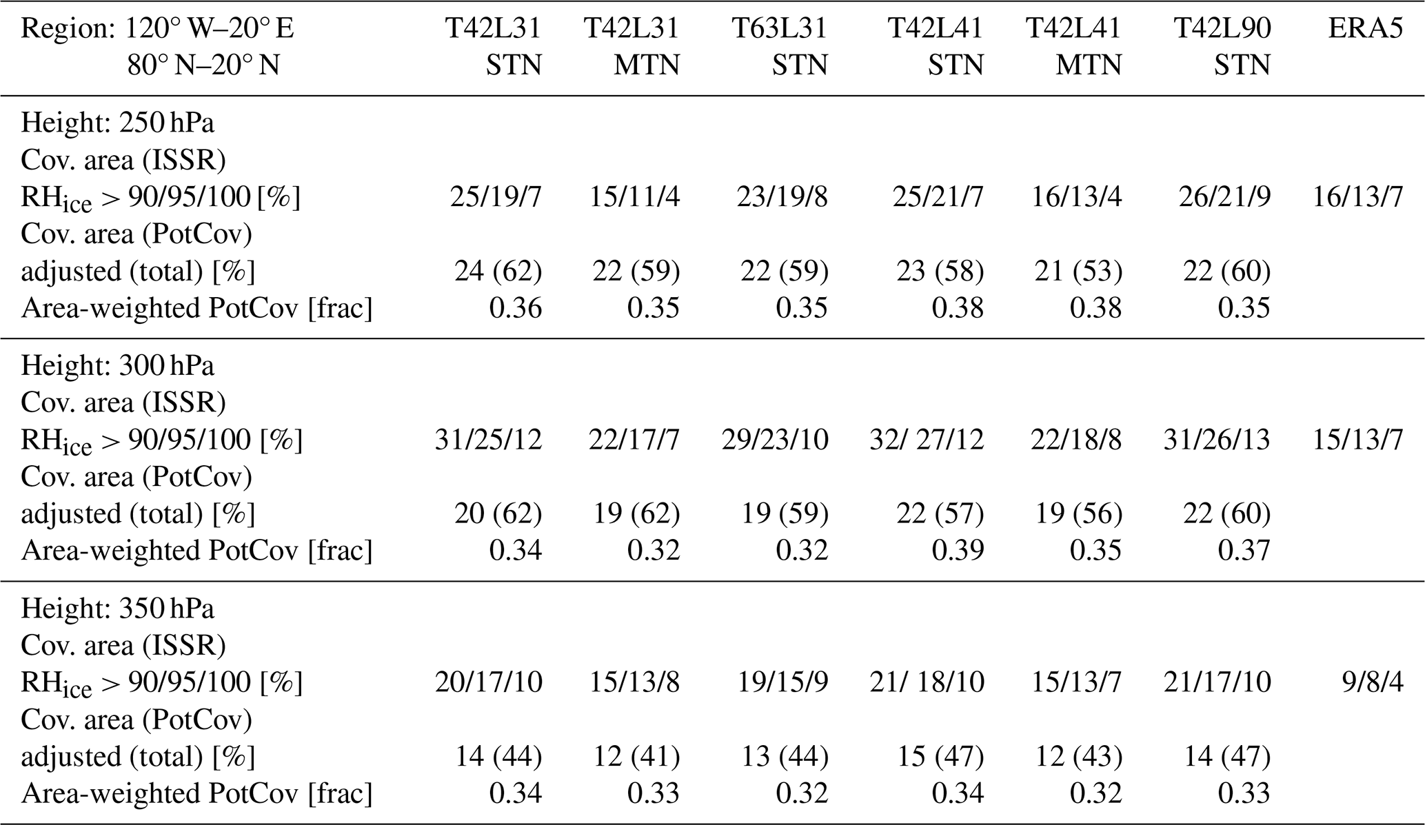
The vertical temperature profiles from EMAC and ERA5 on the specified day (see Fig. S3) display a model cold bias of similar magnitude (3–5 K, peaking around 200–250 hPa) as derived from monthly mean values (Fig. 4). While specific humidity differences exhibit similar patterns, relative humidity distributions show an even larger discrepancy, including cases where the RH_ice of ERA5 exceeds that of EMAC across all setups (see Fig. S8). The findings summarised in Table 2 indicate that both the cold bias in the standard temperature nudged simulations and the overestimation of humidity in the MTN simulations significantly influence the estimated extent of ISSRs. These effects can primarily be attributed to their impact on the calculation of RH_ice. First, the saturation vapour pressure over ice is highly temperature-dependent, decreasing at lower temperatures. This means that colder temperatures result in a lower saturation vapour pressure, requiring less water vapour for the air to reach saturation. As a result, the cold bias leads to an overestimation of regions where contrails can persist and grow, even when the actual RH_ice is below the necessary threshold. Second, a wet bias increases the actual vapour pressure, which also raises the calculated RH_ice, further exaggerating the size of ISSRs. While the choice of nudging method has a significant impact on the results, the number of vertical model levels only affects ISSR predictions at specific pressure levels, highlighting that vertical resolution plays a less critical role in these simulations.

The influence of vertical model resolution and nudging methods on the PotCov approach is also visible in Table 2 for the NAFC. While area-weighted mean PotCov remains consistent across models (0.36 ± 0.02 at 250 hPa, 0.35 ± 0.04 at 300 hPa, 0.34 ± 0.03 at 350 hPa), total coverage varies. At 250–300 hPa, simulations with 31-41 levels show coverage between 59 %–53 %. At 350 hPa, both MTN setups have lower coverage than the STN setups. Summing the geographic grid box areas of those with PotCov greater than zero results is an overestimation of the areas covered with contrails. Therefore, we adjusted the covered area in each grid box with the respective grid box fraction, reducing the potential contrail areas by nearly 60 %. Since this method employs the thermodynamic Schmidt–Appleman criterion, temperature and humidity play a significant role. Variations in these critical parameters account for differences in the resulting covered areas. Furthermore, the vertical resolution appears to have a smaller impact on the areas compared to the previous method. Since the potential contrail parameter is specific to EMAC, direct comparison with ERA5 is not possible. Therefore, we conducted an inter-comparison between both approaches.

The comparison between contrail formation areas based on the ISSR method and the PotCov method reveals the best agreement is at the 95 % RH_ice threshold, although discrepancies persist across different pressure levels. Standard nudged simulations show the closest agreement between both methods at 250 hPa, while simulations with mean temperature nudging perform best at 350 hPa. Specifically, at 250 hPa, MTN underestimates while at 350 hPa STN overestimates the potential contrail areas by 5 %–10 %. Compared to ERA5, the EMAC PotCov method consistently overestimates the covered areas for all pressure levels and model setups, with discrepancies ranging from 1 %–12 %. Our findings suggest that the PotCov approach for mean temperature nudged EMAC data yields the best agreement with ERA5 ISSR areas. However, even with this approach, EMAC simulations result in larger contrail areas compared to ERA5. Furthermore, aside from the discrepancies caused by different nudging approaches, the number of model levels appears to have a negligible impact.

4 Comparison with observations along trajectories (ML-CIRRUS campaign)

In general, the climate impacts of non-CO₂ effects are complex and require detailed knowledge about key atmospheric parameters. Nevertheless, numerous difficulties may arise when modelling parameters such as temperature or humidity using a general circulation model (Jöckel et al., 2016). Consequently, it is advisable to utilise atmospheric measurements to assess model performance in particular regions. Hence, we compared temperature and humidity data on aircraft trajectories obtained during the ML-CIRRUS campaign with the emulated trajectory data from different model setups. It is important to note that the ML-CIRRUS campaign provides in situ measurements along specific aircraft trajectories, representing localised observations, whereas the model results are grid box mean values which represent average conditions over larger spatial areas. To partly account for these differences, we averaged the ML-CIRRUS data over 10 min intervals, aligning with the model output frequency, thereby smoothing the high-frequency variability in the in situ data. This approach allows a more consistent comparison, though some discrepancies may still arise due to the inherent spatial- and temporal-scale differences. From the measurement data, we derive potential contrail formation conditions (e.g. ice supersaturation) that can be compared with EMAC model potential contrail areas and validated with satellite imagery.

4.1 Temperature comparison between EMAC and ML-CIRRUS measurements

All model setups exhibit a high degree of agreement with the observed in situ temperature data from the ML-CIRRUS flights (Fig. 5). To assess this agreement, we first applied spatial resampling by extracting EMAC model data along the aircraft trajectories, followed by temporal resampling of the high-resolution aircraft data to the model's time steps. The resulting time series were then compared, yielding Pearson correlation coefficients (r) between 0.98 and 0.99. This high correlation indicates an excellent correspondence between observed and modelled temperatures. The STN simulations show lower temperatures than the corresponding observations, indicating a constant cold bias of up to 4 K between 200 and 240 K. The simulations show a slope almost equal to 1, consequently producing parallel fitting lines with the central line. The MTN simulations display temperature pairs distributed around the central line with considerable variations of up to 1 K for higher temperatures. Besides that, the 308 data pairs suggest small differences between the MTN setup and the ML-CIRRUS temperature data. Between the simulations with different vertical resolutions, no differences were found in the respective nudging groups. Changing from T42 to T63 horizontal resolution only has a minimal impact and reduces the average bias by a maximum of 0.1 K. A probability density function assessment of only tropospheric and stratospheric data (see Sect. 2.1) indicates the presence of a comparable cold bias in both pressure regions, which is significantly mitigated by utilising the mean temperature nudging method in the simulation (Fig. 5). The differences between the MTN simulation results and the measurements can be attributed to the resampling of observation data and uncertainties during the measurement process. Resampling aligns observational points with model output intervals, which can lead to data smoothing and loss of fine-scale information, especially in rapidly changing conditions. Additionally, measurement uncertainties – such as sensor calibration, environmental factors, and instrumental limitations – impact the precision of observed humidity and temperature values, further contributing to the discrepancies.

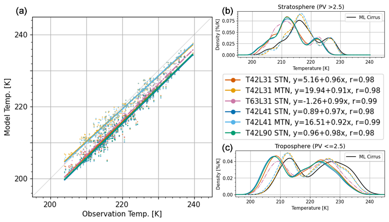
Figure 5 (a) Correlation between temperature data measured during the ML-CIRRUS campaign and simulated using various EMAC model setups at different points along the flight path. Next to the colour bar, the intercept and slope of the linear regression line for each setup are listed, along with the Pearson correlation coefficient (r). (b, c) Probability density function (PDF) of tropospheric temperature data for regions with potential vorticity (PV) ≤ 2.5 (b) and stratospheric temperature data for PV > 2.5 (c). In addition to the different model setups, resampled ML-CIRRUS measurement data (10 min intervals) are shown in black in the PDFs.

4.2 Humidity in EMAC compared to ML-CIRRUS measurements

The analysis of water vapour mixing ratios across various model setups and measurement data, illustrated in Fig. 6, reveals notable discrepancies between model results and observations. For high levels of humidity ranging between 100 and 800 ppmv, predominantly present in the upper troposphere, the results from the standard temperature nudging simulations persistently provide lower values than the HALO FISH and SHARC measurements (see Fig. 6a). This “dry bias” is strongly reduced in simulations with mean temperature nudging (see Fig. 6b). This could be directly connected to the temperature bias reduction found in Fig. 2, as temperature influences humidity. In contrast, for low humidity values between 5 and 10 ppmv, which are located in the lower stratosphere, the model consistently overpredicts compared to the observations by up to 6 times across all model setups. Nevertheless, these low humidity values are not relevant to contrail formation. This model “wet bias” appears with both nudging methods. Overall, the measurements indicate a higher number of data points with water vapour mixing ratio values smaller than 5 ppmv compared to the model. The selection of vertical resolution only has a minor impact on the strength of the correlation. In the lower stratosphere, data from T42L41 show the strongest agreement with the ML-CIRRUS data. This results from the fact that the T42L41 model setup has the highest resolution around the tropopause (refer to Sect. 2.1) in comparison to the other EMAC model setups, which reduces the water vapour diffusion from the troposphere into the stratosphere. For the troposphere, all simulations produce a similar outcome.

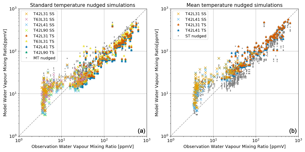
Figure 6 Correlation between water vapour mixing ratio measurements from the ML-CIRRUS campaign and results obtained from different EMAC setups. Standard temperature nudged simulations are coloured in (a), while simulations with mean temperature nudging are shown in grey. In (b), this arrangement is reversed. The respective vertical model resolutions are indicated in red (L31), blue (L41), and green (L90). Stratospheric (SS, crosses) and tropospheric (TS, stars) values are distinguished, with stratospheric values depicted in lighter shades.

4.3 Relative humidity conditions for persistent contrails

We analyse the point-by-point correlation between measurement data and different model setups for atmospheric conditions when contrails can persist longer than a few minutes and significantly impact the climate, following the approach of Gierens et al. (2020). We use the approach discussed in Sect. 2.2 to identify ice-supersaturated regions (ISSRs). To achieve this, we compared RH_ice values derived from FISH and SHARC water vapour mixing ratio and temperature measurements (using Eqs. A1–A3; see Appendix) from the ML-CIRRUS campaign with corresponding data from EMAC. We explore relative humidity thresholds (Dietmüller et al., 2023) by stepwise evaluating categorical statistical measures for model thresholds ranging from 100 % to 90 % (Fig. 7). This comparison (refer to Table 3 for the 90 % threshold) presents values of a 2 × 2 contingency table with four categories: Y/Y (hits), where both ML-CIRRUS and EMAC data indicate conditions that support contrail persistence; Y/N (misses), where ML-CIRRUS measurements predict contrail persistence but the model does not; N/Y (false alarms), where ML-CIRRUS measurements do not predict contrail persistence but the model does; and N/N (correct negatives), where both ML-CIRRUS and EMAC data show that contrail persistence is not possible.

Table 3 Comparison of measured relative humidity with respect to ice derived from ML-CIRRUS data (threshold 100 %) and corresponding data from different EMAC setups (threshold 90 %). The contingency table shows the correlation between the two datasets, including hits (Y/Y), misses (Y/N), false alarms (N/Y), and correct negatives (N/N). The hit rate (HR), expressed as a percentage, represents the proportion of contrail conditions correctly identified by the model (Y/Y) relative to the total measured contrail conditions (Y/Y + Y/N). Conversely, the false alarm rate (FAR), also expressed as a percentage, measures the proportion of incorrectly identified contrail conditions by the model (N/Y) relative to the total measured non-contrail conditions (N/Y + N/N). The equitable threat score (ETS) is a commonly used verification metric that evaluates how well two datasets align by considering not only correct predictions (hits) but also incorrect ones (misses and false alarms). It adjusts for agreements that could occur by chance, providing a fairer measure of predictive skill (refer to Ebert, 1996). The values HR and FAR are illustrated in Fig. 7, together with different threshold between 90 % and 100 %.

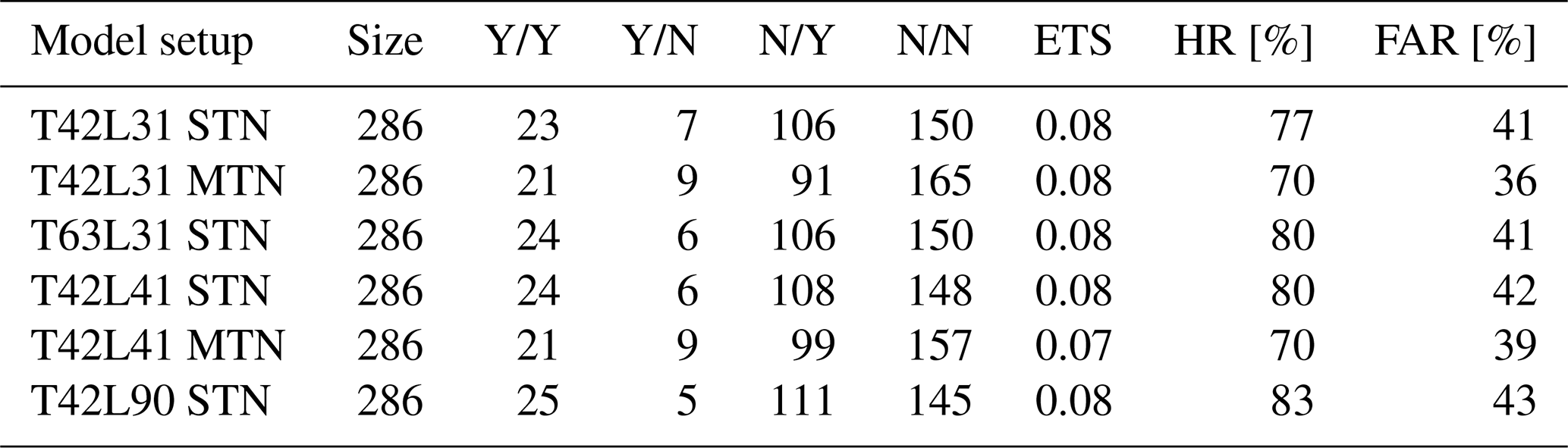
Table 3 reveals that for the selected model RH_ice threshold (90 %), the T42L90 standard nudged model setup achieves the highest hit rate (HR) at 83 %, indicating a strong ability to correctly identify contrail conditions. All standard nudged simulations show high hit rates between 77 % and 83 %, while the mean temperature nudged simulations only show a hit rate of 70 %. Conversely, the MTN simulations exhibit fewer false positives. The T42L31 MTN model achieves a false alarm rate (FAR) of 36 %, the lowest in the table, suggesting the fewest incorrect contrail condition identifications. In over one-third of all cases, the model predicts contrail conditions at this threshold that are not confirmed by measurements, irrespective of the vertical resolution or the nudging approach. The calculations were also performed for other RH_ice thresholds (Fig. 7). Here, the trade-off between sensitivity (hit rate) and specificity (false alarm rate) for different model setups and thresholds becomes apparent. Lower thresholds generally result in higher hit rates and false alarm rates. A false alarm rate below 20 % could only be achieved for RH_ice thresholds over 97 %, with a corresponding hit rate below 50 %. Aiming for high hit rates above 80% increases consequently the false alarm rate to at least 35 % for RH_ice thresholds of 94 %.

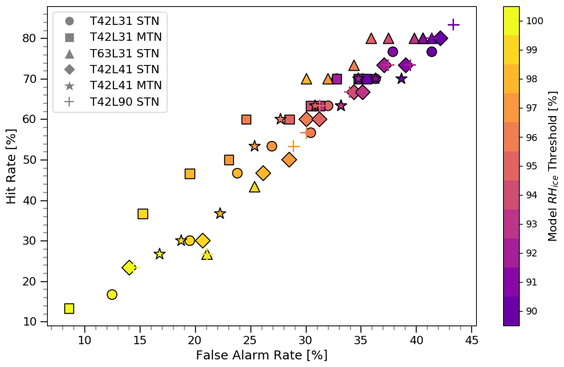
Figure 7 Scatter plot illustrating the relationship between the false alarm rate and hit rate across various model setups and RH_ice thresholds. Each marker type represents a different dataset: circles (T42L31 STN), squares (T42L31 MTN), triangles (T63L31 STN), diamonds (T42L41 STN), stars (T42L41 MTN), and crosses (T42L90 STN). The colour of the markers corresponds to the model RH_ice threshold values, with the gradient ranging from purple (90 %) to yellow (100 %).

At high thresholds, the T42L31 MTN setup performs the best. At lower thresholds (90 %–95 %), the T63L31 and T41L90 setups consistently show higher hit rates than other setups, but they also exhibit higher false alarm rates. The T42L41 setups with standard and mean temperature nudging demonstrate consistent performance with relatively high hit rates and moderate false alarm rates, making them the most balanced model setups. In addition, we also use the equitable threat score (ETS) in Table 3 to characterise the agreement between the datasets. The ETS considers hits, misses, and false alarms while adjusting for random chance, providing a more equitable assessment of forecast performance. The values can be interpreted as follows: ETS = 1 indicates a perfect forecast (all hits, no misses or false alarms), ETS = 0 indicates the forecast is no better than random chance, and ETS < 0 indicates the forecast is worse than random chance. For a detailed explanation of the ETS, refer to Gierens et al. (2020). In our analysis, the ETS values range from 0.07 to 0.08, indicating a low degree of agreement between the two datasets. This suggests that the relationship between the datasets is mostly random and that this statistical analysis does not confirm a clear correlation, which might be due to the small number of data points. By reducing in our analysis both the model and observational relative humidity thresholds below 90 %, more data points are counted as contrail-forming conditions. This increases the number of hits and improves the ETS score to approximately 0.5. However, this artificial enhancement in agreement compromises physical realism, as contrail formation typically requires conditions near full saturation.

5 Case study: ML-CIRRUS flight on 26 March 2014

The analysis of all ML-CIRRUS flights provides important information regarding distinctions between model results and observations. However, these findings do not provide insight into the rapid and abrupt changes in flight level and the subsequent alterations in atmospheric conditions. Additionally, the weather conditions must be considered. Thus, we are monitoring the trajectory of a specific flight to acquire a comprehensive understanding. As a case study, we selected 26 March 2014. Although a polar cold front outbreak occurred across Europe on this date, the region examined here remained largely unaffected by these unusual conditions, maintaining a typical tropopause height of around 200 hPa for this latitude. Moreover, the three flight dives performed on this day allowed us to systematically explore variations between the troposphere and stratosphere and to assess how different dive strengths influenced the observed temperature and humidity profiles. Temperature, humidity, and PotCov are compared along the aircraft trajectory for all EMAC setups. Further, the projected areas of possible contrail coverage are compared with satellite imagery.

5.1 Weather situation during the flight

The weather situation over the North Atlantic on 26 March 2014 shows a relatively weak jet stream, which is limited to the western North Atlantic. High pressure is positioned above Scandinavia, while low pressure dominates across central Europe. Additionally, another low-pressure system is located over southern France and the Mediterranean Sea. At the southern tip of Greenland, a major low-pressure system can be observed, with a warm and a cold front attached, displaying distinct cloud bands across the North Atlantic in the MSG data. In the nudged EMAC simulation, the geopotential height at 500 hPa resembles the reanalysis data of the Deutscher Wetterdienst (Berliner Wetterkarte). PotCov (Fig. 8) is large where the warm and cold fronts are located, although the potential contrail area (Grewe et al., 2014) is considerably more pronounced around the warm front. These results are in line with the observations made by Kästner et al. (1999), who noted that contrail formation is more frequent before warm fronts, before cold fronts, and together with cirrus in a warm conveyor belt.

5.2 S4D sub-model analysis

A direct analysis along the trajectory provides insight into variations in specific atmospheric variables that are not apparent in larger dataset statistics. Figure 9 illustrates a detailed comparison of the parameters throughout the flight. The analysis indicates that the ML-CIRRUS flight on 26 March 2014 was primarily located in the stratosphere with three descents into the troposphere at 08:30, 09:35, and 10:55 UTC. Each of these crossings of the tropopause lasted roughly 45 min and covered pressure differences from 20 to 100 hPa in depth (a). A significant temperature difference between the observations and the model results in both the troposphere and the stratosphere can be observed for the standard nudged simulations. The discrepancy ranges from 3 to 5 K and is minimally affected by the aircraft's ascent or descent. For the simulation with mean temperature nudging (dashed blue and orange lines), this cold bias is not present (b). Regarding tropospheric humidity, lower values are found in the standard nudged simulations compared to the measurement data. However, by applying the MTN method, this bias is largely reduced. In the stratosphere, the models humidity is up to 6 times larger than the measurements, regardless of the nudging method applied. This is particularly noticeable in the first quarter of the flight but can also be seen whenever the aircraft has crossed the tropopause into the stratosphere, i.e. for low humidity values. During the final quarter of the flight, the difference between track pressure and tropopause height is sufficiently large, so that the water vapour mixing ratio values are very low, below 5 ppmv, and there are no significant differences between model results and observation anymore in terms of water vapour mixing ratio (c). All model setups indicate a relative humidity over ice of approximately 100 % in the troposphere for the first two dives, which is consistent with the measurement results. However, during the third dive, the model-predicted RH_ice values exceed the observational data by roughly 20 %. Unlike the previous dives, the third dive occurs further from the tropopause, potentially impacting the accuracy of the model's representation of the relative humidity. In the stratosphere, due to the larger mixing ratio of water vapour visible in panel c, the model simulates a relative humidity over ice between 10 % and 40 %, whereas the observational data are nearly zero in this area. Although this may not significantly impact contrail prediction, as it is far from complete saturation, it does require attention. When contrasting the various model setups, the L41 with mean temperature nudging comes closest to the measurement humidity data (c and d). Based on the temperature and humidity data, contrail formation is expected for the first two dives into the troposphere and partly during the last dive. All model setups predict contrail formation in the troposphere, with some showing a low probability in the lower stratosphere near the tropopause (e). The simulation with the finest spectral (horizontal) but lowest vertical resolution, T63L31, predicts the lowest fraction of possible contrail formation in the tropospheric grid boxes. Applying mean temperature nudging decreases the likelihood of contrail formation for L31 but has no effect on L41, and the overall impact of nudging on PotCov for this specific day is minimal. Differences in PotCov between higher- and lower-resolution setups are partly a consequence of the underlying “contrail cover concept”. This parametrisation, designed to represent partial cloud cover within discrete model grid boxes, can lead to variability that does not solely reflect atmospheric conditions. Instead, it introduces a form of “noise” where changes in resolution and sampling can alter the fraction of the grid box potentially filled with contrails. From this initial analysis, it is not possible to definitively conclude the extent to which these differences stem from systematic resolution effects or from such parametric variability. The impact of the 10 min output interval for the model data compared to the 1 s observational data is significant, as there is a clear delay in the model data after the aircraft's altitude adjustment. Overall, differences in temperature and humidity, which were also observed in the previous sections, can be determined if only this particular day is analysed. A comparison along the trajectory provides insight into the significance of the model output and corresponding resampling interval. It should be noted that the models ability to capture all features observed during the steep dives is limited if the model output interval is too coarse. There is a high level of correspondence between the predicted contrail formation produced by the model and the measured contrail conditions. Between the model configurations, both L41 versions, with or without mean temperature nudging, demonstrate promising results regarding contrail prediction.

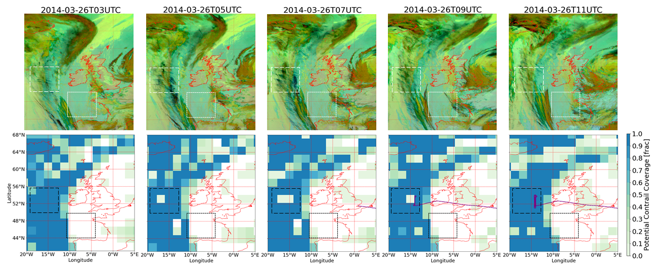
Figure 8 Top: the MSG satellite ash RGB from 20° W to 5° E and 68 to 44° N for 26 March 2014 in 2 h intervals from 03:00 UTC (left) to 11:00 UTC (right). Contrails are visible as dark lines. Bottom: the maximum potential contrail coverage between 300 and 200 hPa (three model levels) derived from the EMAC T63L31 STN model setup. Dark blue indicates high potential grid box coverage, while light green indicates low coverage. The ML-CIRRUS flight track is shown as purple dots. The white and black squares indicate areas with high (–) and no (…) contrail coverage.

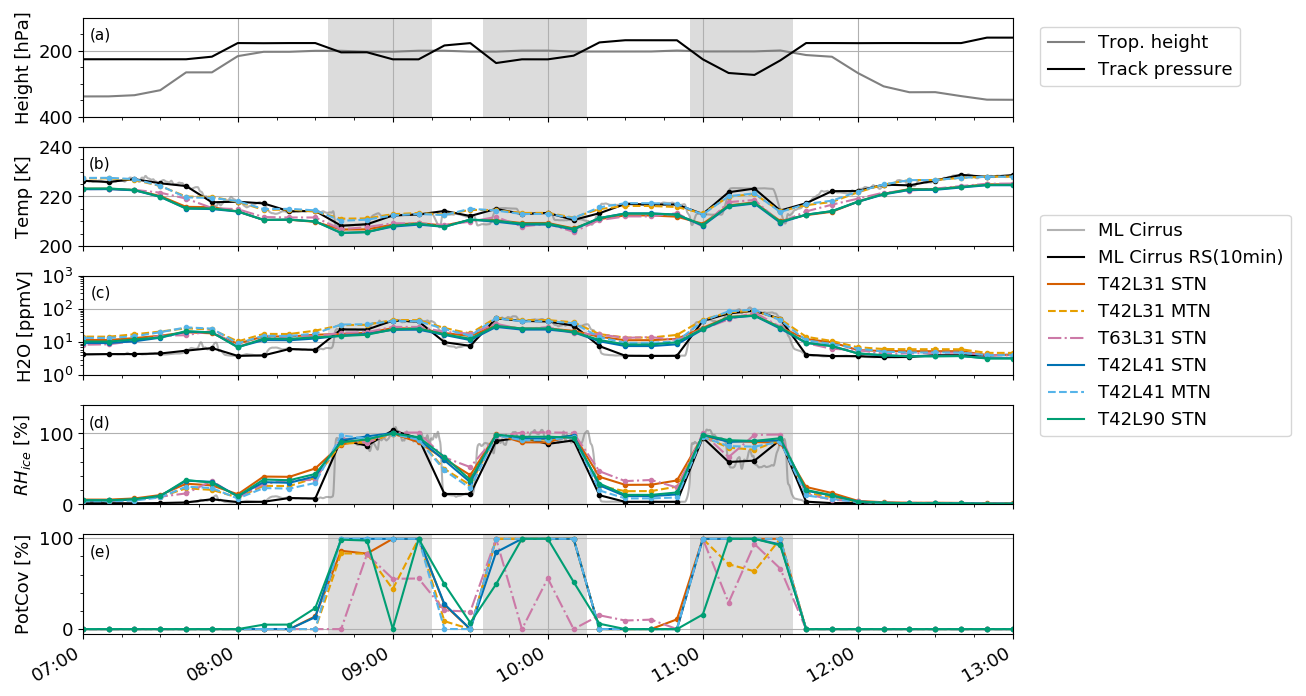
Figure 9 Comparison of various atmospheric parameters along the flight trajectory for 26 March 2014. (a) Tropopause height and the track pressure height of the HALO aircraft. Comparison of temperature (b), water vapour mixing ratio (c), and relative humidity with respect to ice (d) between results obtained with different EMAC setups and ML-CIRRUS measurements (FISH and BAHAMAS). Panel (e) shows the predicted contrail coverage in EMAC for the according grid box.

5.3 Potential contrail coverage and satellite observations

The satellite image (top panel in Fig. 8) shows a ridge cloud on 26 March 2014 composed of a cloud band extending from Iceland southwards passing west of Ireland and Great Britain. Contrail lines are best observed in correspondence to the cloud band over a wide range of latitudes starting east of Iceland and north of Scotland and ending east of Portugal, with many contrails east of Scotland and Ireland and fewer contrails south of Ireland. The spread of these contrail lines is strongly influenced by large-scale synoptic weather patterns. Although the areas where contrails were observed remained consistent throughout the observed time span of 8 h, a notable increase in intensity occurred at 05:00 and 07:00 UTC, coinciding with the period when air traffic from the United States to Europe is passing these regions. Of course, contrails can only form where aircraft fly. The maximum PotCov in the T63L31 STN model indicates the highest value is observed between 300 and 200 hPa (bottom panel in Fig. 8). This analysis reveals that the distribution of PotCov follows the distribution of the ridge cloud in the ash RGB. EMAC indicates the ridge cloud as location of potential contrail formation, which is plausible in comparison to the satellite picture. Additionally, areas where no contrails are predicted, such as south of Ireland, correspond to regions with no observed satellite contrail coverage. As the ML-CIRRUS campaign conducted measurements east of Ireland on this day, the observed area of contrail formation can also be linked to high relative humidity over ice values. Further regions of high potential contrail areas, e.g. over south Scandinavia and north of Corsica, cannot be evaluated with these satellite observations because no contrails are observed here. The region east of England with high potential cloud coverage is also difficult to evaluate because the few dark lines in the ash RGB in this region (see e.g. 05:00 UTC) cannot be unambiguously attributed to contrails.

6 Discussion

The results presented here highlight the strong influence of temperature and relative humidity fields on contrail formation and persistence. Accurate representation of these parameters is crucial for realistic contrail modelling. Our analysis reveals a persistent cold bias of 3–5 K in standard nudged EMAC setups across various vertical and horizontal resolutions and geographic regions. This bias likely stems from known limitations in general circulation models, as previously noted by Stenke et al. (2007). Notably, the introduction of mean temperature nudging (MTN) techniques reduces this bias, aligning the EMAC temperatures with ERA5 reanalysis data and improving agreement with in situ measurements from the ML-CIRRUS campaign. The minimal improvements gained by increasing model horizontal resolution from T42 to T63, paired with substantially higher computational costs, suggest that simply refining spatial resolution does not address fundamental biases. Instead, targeted strategies such as MTN prove more effective in correcting systematic errors, thereby enhancing confidence in contrail predictions.

However, such mean temperature nudging has potentially adverse effects on the radiation balance or the hydrological cycle (Jöckel et al., 2016), as no recalibration was performed. This effect becomes apparent when analysing the specific humidity results. Humidity poses a challenge in climate modelling due to its spatial and temporal variability. It is noteworthy that specific humidity is overestimated in models such as the ECMWF’s Integrated Forecasting System (IFS), while humidity over-saturation is underestimated in this model (Krüger et al., 2022; Woiwode et al., 2020; Reutter et al., 2020). The latter has a significant impact on contrail formation (Gierens et al., 2020). Overall, earlier studies have shown that the EMAC model underestimates water vapour due to its cold bias (Brinkop et al., 2016; Jöckel et al., 2016). Our simulations reveal similarly that water vapour mixing ratios are consistently underestimated between 50 and 400 hPa, except for the tropopause region at around 200 hPa, where the EMAC model actually overestimates water vapour mixing ratios compared to ERA5. The difference between the ERA5 and EMAC increases towards the poles, with the two EMAC setups that include mean temperature nudging displaying an even larger deviation from ERA5. An explanation for this is that there is a rise in the wet bias in the extra-tropical area which occurs due to water vapour diffusing horizontally from the tropical upper troposphere into the extra-tropical lowermost stratosphere. This phenomenon was also noted by Stenke et al. (2007). While the exact cause of the observed wet bias for the MTN simulations at higher altitudes remains uncertain, it may be related to the wave-zero temperature nudging forcing the model away from its internal equilibrium, prompting compensatory adjustments in humidity fields. Further dedicated analyses or sensitivity simulations, beyond the scope of this study, would be needed to substantiate this explanation. The overestimation is also evident in the comparison with observational data. The difference is significant for lower water vapour mixing ratios, which are typically present close to the tropopause. Aircraft often cross this region without flying directly along the tropopause. This results in very small sample sizes, which, in combination with strong lapse rate changes, make it a difficult region to evaluate. To evaluate model performance, we compared EMAC output with in situ measurements from the ML-CIRRUS campaign. Although a persistent temperature bias is noted in the model, the comparison is considered robust. Recent findings have provided new insights into the anti-ice (AI) correction for aircraft temperature measurements (Giez et al., 2023), indicating a possible cold bias in the temperature data, which we want to discuss here. The static air temperature on aircraft is determined using a total air temperature (TAT) probe, which measures the temperature of the air impacted by the aircraft's motion. This probe is housed within a sensor inlet (e.g. Collins Aerospace 102BX) that is actively heated to prevent ice formation, a process known as anti-icing. Ice accumulation on the inlet can lead to erroneous temperature measurements under in-flight icing conditions. The heating affects the temperature readings inside the housing, necessitating a correction known as the anti-ice (AI) correction. While the manufacturer provides a parameterised correction for this effect, the AI correction for the HALO aircraft was determined individually through in-flight calibration (Bange et al., 2013). During the ML-CIRRUS campaign, no AI correction was applied to the measurement data, based on experimental evidence suggesting it was unnecessary. However, recent test campaigns have shown that this does not hold for all flight conditions. The correction is generally negligible, with a value of less than 0.1 K across most flight conditions. However, it becomes significant at very high altitudes with low speeds, which are not typical flight conditions for the HALO aircraft. The application of the AI correction results in a slightly lower static air temperature, but this correction remains within the specified error margins for temperature measurements. Therefore, the temperatures calculated during the ML-CIRRUS campaign are likely unaffected by the new AI correction. Contrail formation can be identified through two main approaches: one based solely on ice-supersaturated regions (ISSRs) and another employing the SAC to derive potential contrail coverage (PotCov). Both require similar microphysical conditions (temperature and humidity thresholds), but the SAC-based approach is more physically comprehensive as it includes aircraft engine parameters such as propulsion efficiency and specific fuel combustion heat (Schumann, 1996; Schumann et al., 2000; Grewe et al., 2014). While the simpler ISSR-based method can identify where contrails may form, the SAC-based approach is generally considered more refined and potentially more accurate, as it directly links aircraft properties and ambient conditions. Consequently, varying these aircraft parameters can influence the spatial extent and frequency of predicted contrails. For instance, adjusting the propulsion efficiency would have a relatively small effect on contrail formation regions, while changes to parameters like the emitted water vapour could more substantially alter the predicted contrail coverage. As demonstrated in frameworks like CoCiP (Schumann, 2012), an accurate representation of engine and fuel parameters can significantly improve the realism of contrail predictions and thus inform us about more effective climate mitigation strategies in aviation.

Despite significant differences in water vapour mixing ratios, simulations with mean temperature nudging show smaller absolute differences in relative humidity over ice compared to ERA5 than those with standard nudging. However, both simulations display higher values than the reanalysis data. This indicates that the model temperature bias has a stronger effect on the relative humidity over ice than the model wet bias. Both biases directly impact predicted ice-supersaturated regions, which are crucial for the contrail life cycle. Simulations with standard nudging show larger areas for contrail formation compared to ERA5 across all relative humidity over ice thresholds. However, prior research has found that lower thresholds such as 90 % (Dietmüller et al., 2023) or 93 % (Hofer et al., 2024) achieve better agreement between observations and the ERA5 model results. This is consistent with the present study, where we found the highest correlation between the PotCov areas calculated online during the simulations and the ISSR areas derived offline with a RH_ice threshold of less than 96 %. The order of magnitude of the identified area on the case study day is consistent with the ISSR occurrence results reported by Petzold et al. (2020) for 250 and 300 hPa, where they observed ISSR frequencies of occurrence of 19 % and 25 %, respectively.

While the agreement between ERA5 and the various EMAC setups with respect to potential contrail coverage areas remains within 10 %, the difference compared to direct observations is larger. The point-by-point comparison between ML-CIRRUS measurements and EMAC model outputs for regions suitable for persistent contrail formation indicates no correlation (low ETS scores) when the model threshold is set to 90 % and the observation threshold remains at 100 %. Although our limited sample size (286 data points) may partly explain the low skill, more fundamental reasons are likely behind these results. This threshold pairing yields similar hit rates and false alarm rates across all model setups. Adjusting the model RH_ice threshold significantly affects both metrics: generally, higher thresholds increase both hit and false alarm rates. However, keeping the false alarm rate under 20 % is preferable to avoid unnecessary re-routing and increased climate impact. Achieving such a low false alarm rate often reduces the hit rate to below 50 %, meaning many areas that could actually support contrail formation remain undetected. Despite this trade-off, it is still better to accept a lower hit rate than to tolerate frequent false alarms. Note that the RH_ice thresholds from Dietmüller et al. (2023) and Hofer et al. (2024), which yield better verification scores, apply to ECMWF data, and EMAC may require its own optimised threshold. While contrail cirrus can persist below 100 % RH_ice (Li et al., 2023), the initial formation phase typically requires conditions near saturation. Thus, our use of a 100 % observational threshold is physically justified, and lower tested thresholds were intended only to assess model sensitivity. Beyond threshold issues, comparing localised in situ aircraft measurements to grid-box-averaged model fields remains challenging, and the identified temperature and humidity biases also influence the ETS scores. In line with our findings, Gierens et al. (2020) reported low correlations between model data (ERA5) and aircraft measurements (MOZAIC). Even ERA5, which generally aligns more closely with our contrail metrics, may exhibit its own humidity biases (Charlesworth et al., 2023). Moreover, the complexity of modelling contrails – from small-scale humidity fluctuations to the representation of aircraft engine parameters – further limits the skill of direct comparisons.

Future improvements could involve refining the RH_ice thresholds specifically for EMAC or exploring bias correction techniques to better align the model’s humidity fields with observations (Teoh et al., 2024). Integrating more comprehensive observational datasets, such as additional flight campaigns or satellite-based humidity measurements, might help reduce uncertainties. Enhancing data assimilation methods and adjusting model parametrisations could also yield more accurate contrail predictions. Ultimately, addressing these limitations and refining the underlying assumptions will be key steps toward achieving higher skill scores and more reliable contrail forecasts in future studies. Since the Schmidt–Appleman criterion, a thermodynamic theory that has been thoroughly tested and validated, is the basis for the PotCov calculation in EMAC, any deviations in contrail coverage mainly arise from inaccurate representations of key parameters for contrail formation, such as temperature or humidity. Changes to the horizontal or vertical resolution of the model had only little effect on the outcome. Future studies need to evaluate the impact of the transition from the bi-linear interpolation to the nearest-neighbour approach. Despite the fact that the 41-layer setup simulates the best agreement with observations, it still does not cover atmospheric processes in the stratosphere well, which could consequently have a minor influence on contrail prediction. However, this study reveals that this does not significantly impact the results, as all three model setups have the same model grid resolution of approximately 450 m vertically in the UTLS region, resulting in similar results. The cold and humidity biases present in all regions of the Northern Hemisphere that were shown in this study may not only affect contrail formation region predictions but also have an impact on the water cycle, cloud formation, and the radiation budget. Despite the model’s biases, the predicted contrail formation areas closely match those observed in satellite imagery. From 03:00–05:00 UTC, we find close agreement in both the high-coverage contrail regions and the regions without contrails. We attribute this agreement to atmospheric conditions being sufficiently far from critical thresholds for contrail formation, so temperature and humidity biases do not significantly affect the ISSR evaluation. Later in the day, from 07:00–09:00 UTC, we find only partial agreement in the high-coverage contrail regions, likely due to atmospheric conditions being closer to the formation threshold. Under these conditions, any model bias affects the ISSR evaluation, and areas where contrails are observed are not consistently captured by the model. Although the global mean temperature nudging used in EMAC may not directly translate to operational numerical weather prediction (NWP) systems, the overarching conclusions remain relevant. NWP models could employ improved data assimilation, bias correction strategies, and carefully chosen RH thresholds to enhance contrail forecasting. By doing so, future operational frameworks might better integrate contrail avoidance measures, ultimately contributing to climate-optimised flight operations.

7 Summary and conclusions

This study enhances the understanding of contrail prediction limitations in the global climate model EMAC and evaluates categorical statistical measures related to temperature and humidity biases in different EMAC setups. We evaluated several EMAC model setups with various vertical resolutions (L31, L41, L90), horizontal resolutions (T42, T63), and different nudging approaches (STN, MTN) regarding their ability to identify regions of the atmosphere where contrails can form and persist. We assessed temperature and humidity biases and their influence on contrail prediction by comparing EMAC outputs with ERA5 reanalysis data, satellite observations, and in situ flight measurements from the ML-CIRRUS campaign. A consistent cold bias of 3–5 K was identified in the standard nudged EMAC model (STN) between 100 and 400 hPa. This bias was observed across the Northern Hemisphere, independent of latitude or region, and persisted across all investigated vertical and horizontal resolutions. It aligns with past findings related to the upper boundary conditions in general circulation models. Since contrails require sufficiently low ambient temperatures (around 235 K) to form, this cold bias leads to an overprediction of contrail-forming regions. It also results in an overestimation of relative humidity over ice, enlarging identified ISSRs and thereby affecting contrail persistence. Implementing global mean temperature nudging (MTN) significantly reduces the cold bias, bringing EMAC outputs closer to ERA5 and ML-CIRRUS temperature measurements. However, it also introduces a positive humidity bias, which increases the extent of ISSRs and ultimately leads to an overestimation of contrail persistence. Despite the differences identified in temperature and humidity, the model’s cold bias has only a minor impact on large-scale contrail formation, as aircraft flights predominantly occur in regions where ambient temperatures are well below the critical threshold. All three vertical resolutions (L31, L41, L90) reproduce the extent of regions where persistent contrails can form, with an overestimation of less than 10 percentage points compared to ERA5 data. Consequently, EMAC reliably identifies potential contrail-forming regions, demonstrating its suitability for contrail studies. The small reduction in temperature bias observed when increasing the horizontal grid resolution from T42 to T63 – along with a reduction in ISSR areas – was not significant enough to justify the substantially higher storage and computational costs. It should be noted that the analysis is limited to a single spring season in 2014. Nevertheless, the temperature and humidity biases identified in this study contribute to forecast uncertainties in contrail modelling, which need to be addressed when predicting ISSRs in atmospheric models. These uncertainties form the basis for risk assessments when implementing contrail avoidance strategies or climate-optimised trajectories. By extending existing climate change functions (CCFs) to different seasons and geographical regions, future studies can better quantify how such uncertainties vary over time and space. One approach to reduce the temperature bias explored in this study is mean temperature nudging. However, the physical inconsistencies introduced by MTN led to new issues related to humidity. Future work should focus on carefully tuning MTN setups toward a realistic radiation balance, as this method strongly affects both humidity and the radiation budget. Failure to address these issues could render the model unsuitable for quantifying the climate impact of contrails. Similar to nudging, the assimilation of realistic temperature and humidity data in NWP models offers a promising approach to reducing model biases through observational data, which should be further explored in future studies.

Appendix A: Relative humidity and water vapour mixing ratio

The relative humidity with respect to ice RH_ice is a model parameter required to identify areas where contrails can form. This value relies on the specific humidity (SH), temperature (T), and pressure (P) and can be expressed as the ratio of the water vapour pressure (VP) to the saturation pressure over ice SP_ice (see Eq. A1).

$$\begin{array}{}\text{(A1)}& {\mathrm{RH}}_{\mathrm{ice}}=\mathrm{100}\cdot {\displaystyle \frac{\mathrm{VP}}{{\mathrm{SP}}_{\mathrm{ice}}}}\end{array}$$

With the ratio of molar mass of water to molar mass of dry air (ε) being a constant of 0.622, the water vapour pressure is solely dependent on specific humidity and pressure and is directly proportional to these variables (Eq. A2), while the saturation pressure over ice can be estimated by the temperature (Eq. A3, based on Murphy and Koop, 2005) – with the temperature being inversely proportional to the relative humidity.

$$\begin{array}{}\text{(A2)}& {\displaystyle }\mathrm{VP}={\displaystyle \frac{P\cdot \frac{\mathrm{SH}}{\mathrm{1}-\mathrm{SH}}}{\mathit{\epsilon }+\frac{SH}{\mathrm{1}-\mathrm{SH}}}}\text{(A3)}& {\displaystyle }\begin{array}{rl}{\mathrm{SP}}_{\mathrm{ice}}& =\exp (\mathrm{9.550426}-{\displaystyle \frac{\mathrm{5723.265}}{T}}+\mathrm{3.53068}\\ & \cdot \log \left(T\right)-\mathrm{0.00728332}\cdot T)\end{array}\end{array}$$

This can be demonstrated in a simple example: when applying typical atmospheric values (temperature = 215 K, specific humidity = 3.5 × 10⁻⁶ kg kg⁻¹, pressure = 250 hPa) to Eq. (A1), the resulting relative humidity is approximately 101 %. If the temperature is reduced by 5 to 210 K (2.5 %), while all other parameters are kept constant, the relative humidity over ice rises to 200%. Alternatively, if the specific humidity doubles to 7 × 10⁻⁶ kg kg⁻¹, the relative humidity once again increases beyond 200 %. Summarised, a decrease in temperature or increase in specific humidity will result in an increased relative humidity. The water vapour mixing ratio (MR) is calculated from the specific humidity (SH) values in the model, using Eq. (A4); ϵ is the relation of molar mass of water to the molar mass of dry air (0.622).

$$\begin{array}{}\text{(A4)}& \mathrm{MR}={\displaystyle \frac{\mathrm{1}}{\mathit{\epsilon }}}\cdot {\displaystyle \frac{\mathrm{SH}}{\mathrm{1}-\mathrm{SH}}}\end{array}$$

The calculation is necessary for the comparison with humidity data from the ML-CIRRUS campaign, given as the water vapour mixing ratio.