Explaining the period fluctuation of the quasi-biennial oscillation

The tropical stratosphere is characterized by a periodic oscillation of wind direction between westerly and easterly, known as the quasi-biennial oscillation (QBO), which modulates middle atmospheric circulations and surface climate on interannual timescales. The oscillation period fluctuates irregularly, ranging from 20 to 35 months. The causes of this fluctuation have long been hypothesized but lack observational evidence. This study shows that the period fluctuation is primarily driven by variability in small-scale wave (gravity wave) activity with an additional contribution from variability in tropical upwelling. Using an atmospheric reanalysis dataset, we capture temporal variations in small-scale wave activity that are coherent with the varying speed of the oscillation. This wave activity variation stems from the seasonality of tropical convection and tropopause layer wind, revealing their fundamental role in modulating the quasi-biennial period. Our findings suggest that better representing these multiscale interactions in models can enhance the accuracy of seasonal forecasts and the reliability of future climate projections.

1 Introduction

The wind in the tropical stratosphere alternates between an easterly and westerly direction with periods varying irregularly from 20 to 35 months (Baldwin et al., 2001; Anstey et al., 2022a). This so-called quasi-biennial oscillation (QBO) is intense enough in amplitude (∼30 m s⁻¹) to modulate the extratropical circulation and global distributions of chemical species (e.g., Holton and Tan, 1980; Ling and London, 1986; Randel and Wu, 1996; Kinnersley and Tung, 1998; Flury et al., 2013). The alternating wind phases propagate down to the tropopause layer (∼18 km altitude). Recent studies have revealed further downward impacts of the QBO on surface weather and climate in the tropics (Haynes et al., 2021; Yoo and Son, 2016) and extratropics through atmospheric teleconnections (Thompson et al., 2002; Garfinkel and Hartmann, 2011; Gray et al., 2018; Anstey et al., 2022b). The QBO is therefore regarded as an important climate mode that can enhance the skill of seasonal and decadal predictions, provided that it is reproduced well by forecasting models (Scaife et al., 2014; Coy et al., 2022).

A barrier to the successful prediction of the QBO is the variability in its period and phase progression. The speed of phase progression varies, largely depending on the calendar month, and accordingly, the lengths of individual oscillation cycles fluctuate (e.g., Dunkerton, 1990; Wallace et al., 1993; Schenzinger et al., 2017; Coy et al., 2020). Current seasonal prediction models are deficient in capturing the varying timings of phase transition, which limits the forecast skill of the oscillation beyond the lead time of a few months (Stockdale et al., 2022; Coy et al., 2022). In line with this, climate models tend to reveal a lack of variability in the QBO period in multi-decadal simulations (Bushell et al., 2022). Regarding this problem, a fundamental question is the underlying process driving the observed fluctuations in the period and phase-progression speed, which remains unresolved.

The QBO is primarily a dynamic phenomenon driven by momentum forcing due to atmospheric waves (Lindzen and Holton, 1968; Holton and Lindzen, 1972). Observational and theoretical studies have demonstrated that a broad spectrum of atmospheric waves, generated by heat release from tropical convection, propagates vertically into the stratosphere (e.g., Holton, 1972; Salby and Garcia, 1987; Horinouchi and Yoden, 1996; Song et al., 2003; Song and Chun, 2005). They transport and deposit momentum to the flow in the stratosphere around the easterly or westerly jet of the QBO. This acts as the restoring force of the oscillation, advancing its phase (Lindzen and Holton, 1968; Holton and Lindzen, 1972). However, the flow in the tropical stratosphere is not purely horizontal but weakly upward on average (by less than 1 mm s⁻¹) (Schoeberl et al., 2008; Kim and Chun, 2015b). Albeit very slow compared to horizontal motions, this upwelling advects substantial momentum, which can largely offset the wave forcing, thereby retarding the oscillation. Therefore, the theoretical hypothesis suggests that the fluctuation in the QBO progression speed could be explained by variations in the magnitude of upwelling and/or wave activity (e.g., Dunkerton, 1990; Kinnersley and Pawson, 1996; Hampson and Haynes, 2004; Kim et al., 2013; Krismer et al., 2013; Anstey et al., 2022a).

To date, no observational evidence has been found for the coherent variation of the wave activity with the fluctuating QBO periods (for a climate model result, see Krismer et al., 2013). A difficulty has existed in this issue because of the limitations of measurements in spatial resolution and coverage, given the ubiquitous convection over the tropics and the broad wave spectrum down to the ∼10 km scale in horizontal wavelength. On the other hand, the stratospheric upwelling is known to have a seasonal cycle (Mote et al., 1996, 1998; Schoeberl et al., 2008), and its possible effects on the QBO variability have been extensively studied using observational records and modeling approaches (e.g., Kinnersley and Pawson, 1996; Hampson and Haynes, 2004; Rajendran et al., 2018; Coy et al., 2020). In particular, it has been suggested that the seasonal dependence of QBO progression, including its stalling (Wallace et al., 1993; Kinnersley and Pawson, 1996), could result from the seasonal cycle of the upwelling. In addition, the decadal-scale modulation of the QBO period by the solar cycle has also been proposed, potentially linked to the solar effect on global stratospheric circulation, including tropical upwelling (Salby and Callaghan, 2000; Pascoe et al., 2005). However, subsequent observations have shown that the relationship between the solar cycle and the QBO is inconsistent over time and remains uncertain (e.g., Fischer and Tung, 2008).

Here, we use global reanalysis data to investigate the fluctuations in the QBO period and progression speed. Our study reveals the underlying process driving these fluctuations, providing new evidence of the coherent variation of small-scale wave activity with the QBO periods.

2 Data and methods

2.1 Datasets

European Centre for Medium-Range Weather Forecasts (ECMWF) Reanalysis version 5 (ERA5, Hersbach et al., 2020) data were used throughout the study. ERA5 is a global reanalysis spanning 1940 onward with a spatial resolution of ∼30 km. We used hourly wind and temperature data for the period of 1956–2015. The analysis period was determined to begin with the first observation of the QBO up to 10 hPa altitude. We excluded years after 2015 because the oscillation phases could not be unambiguously defined due to the QBO disruptions which occurred in 2016 and 2019–2020 (e.g., Osprey et al., 2016). The conventional pressure-level dataset was used for all analyses (such as wave momentum fluxes and momentum forcing, described in Sects. 2.3 and 2.4), except for calculating the QBO-phase descent speed and the 84 hPa wave flux (Sect. 4.1). For the descent speed, finer vertical profiles of monthly zonal wind were obtained from the ERA5 native model-level dataset. For the annual cycle of precipitation, the long-term mean data from the Global Precipitation Climatology Project (GPCP) Monthly Analysis version 2.3 (Adler et al., 2003) were used.

2.2 QBO cycles and periods

Monthly and zonally averaged zonal winds over 5° N–5° S were used to describe the QBO. At each height, we defined an oscillation cycle as the period between the onsets of westerly winds. To avoid noise around zero wind and uniquely detect the onset of westerly winds, the monthly time series was smoothed through three iterations of the three-point moving average with coefficients $[\mathrm{1},\mathrm{2},\mathrm{1}]/\mathrm{4}$ but only when defining the cycle.

2.3 Wave momentum fluxes

Upward fluxes of eastward and westward momentum due to waves were calculated monthly, after decomposing waves via the Fourier transform in longitude and time. For the two-dimensional Fourier transform, a 34 d window centered on the target month was used, with sine-tapering applied over 4 d on each side (leaving the central 26 d untapered). The eastward (westward) momentum fluxes were obtained by summing positive (negative) zonal-momentum fluxes in the Fourier domain where the zonal phase speeds were positive (negative). Absolute values were taken for the westward momentum fluxes.

In this study, we refer to small-scale waves as those with zonal wavenumbers greater than 20 (wavelengths less than ∼2000 km, i.e., gravity waves). When analyzing momentum fluxes of small-scale waves, only waves with zonal phase speeds greater than ±5 m s⁻¹ were considered. Local ambient winds for small-scale waves vary zonally in the tropical upper troposphere (e.g., due to the Walker circulation), allowing for both eastward and westward momentum fluxes at a given low phase speed, depending on the location of the waves. The phase-speed threshold (±5 m s⁻¹) was applied to avoid artificial variability in the calculated momentum fluxes, as fluxes in opposite directions would offset each other in the spectrum at low phase speeds.

2.4 Momentum forcing

The change rate of zonally averaged wind is expressed as

$$\begin{array}{}\text{(1)}& {\displaystyle }{\displaystyle \frac{\partial \stackrel{\mathrm{‾}}{u}}{\partial t}}={\displaystyle \frac{\mathrm{\nabla }\cdot \mathit{F}}{{\mathit{\rho }}_{\mathrm{0}}a\cos \mathit{\varphi }}}-{\stackrel{\mathrm{‾}}{w}}^{*}{\displaystyle \frac{\partial \stackrel{\mathrm{‾}}{u}}{\partial z}}+{\stackrel{\mathrm{‾}}{v}}^{*}\widehat{f},\end{array}$$

by defining the Eliassen–Palm (EP) flux F and meridional and vertical velocities of the residual circulation $({\stackrel{\mathrm{‾}}{v}}^{*},{\stackrel{\mathrm{‾}}{w}}^{*})$ following Andrews et al. (1987). Here, ρ₀, a, and (ϕ,z) are the reference density, earth radius, and latitudinal and vertical coordinates, respectively; $\widehat{f}:=f-(a\cos \mathit{\varphi }{)}^{-\mathrm{1}}\partial (\stackrel{\mathrm{‾}}{u}\cos \mathit{\varphi })/\partial \mathit{\varphi }$, where f is the Coriolis parameter. The first two terms on the right-hand side of Eq. (1) represent the major components of momentum forcing in the equatorial stratosphere: total wave forcing (contributed by waves of all scales) and vertical advection by upwelling, respectively. The terms in Eq. (1) were calculated using hourly data and averaged monthly. Additionally, an indirect estimate of the total wave forcing was also obtained by subtracting all terms except the first on the right-hand side from the wind change rate in Eq. (1).

3 Characteristic behaviors of the QBO

Figure 1a shows the QBO of the tropical stratospheric wind with alternating phases, highlighting a large variation in its period (horizontal arrows) in the late 1990s–early 2000s (see Fig. 2 for the record of QBO periods since 1956). A characteristic phenomenon associated with the period variation is the change in the descent speed of the easterly phase (Fig. 1a). The downward propagation of this phase often stagnates, as observed in the period from late 2000 through early 2001, resulting in a lengthening of the oscillation cycle. However, the downward speed of the westerly phase barely changes between cycles or within each cycle, as measured by the slopes of the zero-wind lines at the bounds of cycles in Fig. 1a. This results in the period of each cycle being nearly constant with height.

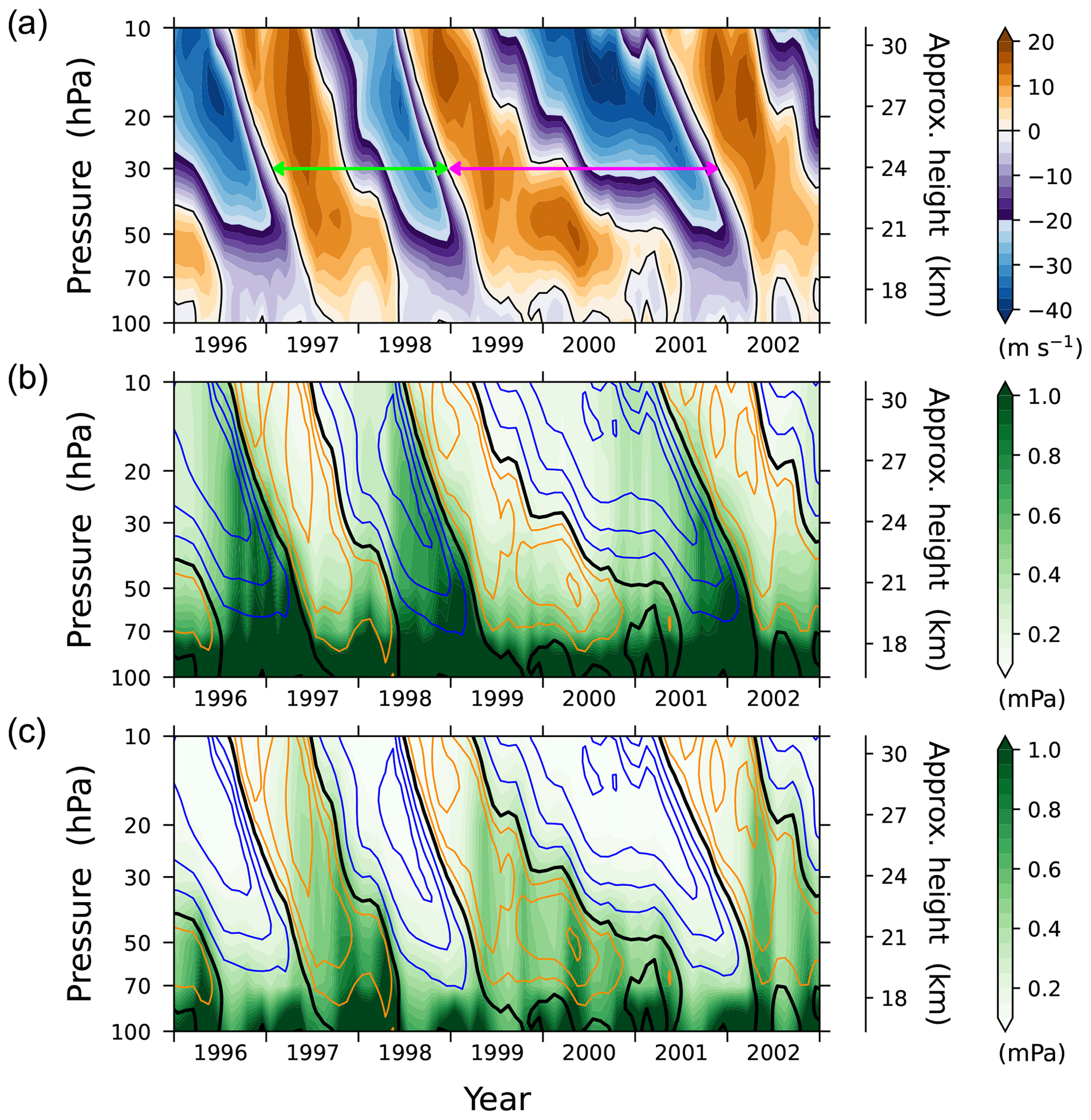
Figure 1 (a) Stratospheric zonal wind velocity averaged over 5° N–5° S. The green and magenta arrows indicate two examples of oscillation cycles at 30 hPa, highlighting a large variation in the QBO period. (b, c) Upward fluxes of (b) eastward and (c) westward momentum due to atmospheric waves (shading), averaged over the same latitude band, along with the wind (yellow contours for westerlies at 5 m s⁻¹ intervals; blue contours for easterlies at 10 m s⁻¹ intervals; thick black contours for zero winds).

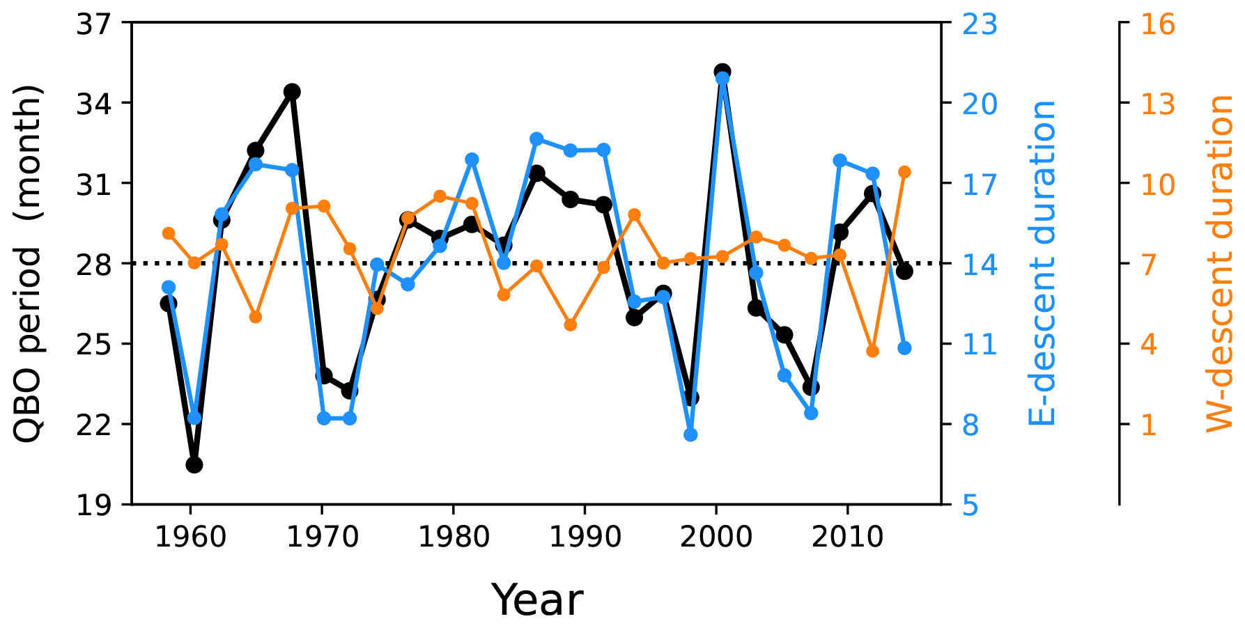
Figure 2 QBO period measured at 30 hPa (black), along with the durations of the easterly-phase (blue) and westerly-phase (orange) descent from 15 to 50 hPa, for the QBO cycles over 1956–2015. The averages of the three variables over the cycles (28, 14, and 7 months, respectively) are indicated by the dotted horizontal line. Pearson correlation between QBO periods and easterly-phase descent durations is 0.91.

Another characteristic of the QBO is that the onset of westerly phases at 10 hPa roughly coincides with the end of those phases at about 70 hPa (near the bottom of the tropical stratosphere), and the same pattern holds for easterly phases (Fig. 1a). This can be explained by the established theory of the interaction between atmospheric waves and flow (Holton and Lindzen, 1972; Plumb, 1977). Figure 1b shows upward fluxes of eastward momentum carried by the waves. The eastward momentum fluxes are largely reduced under the westerly flow condition, as the theory suggests. Therefore, at an arbitrary altitude, these fluxes can be substantial only when the flow is easterly throughout the layer below. The formation of such an easterly layer by the cessation of the westerly phase at 70 hPa allows eastward momentum to be transported to ∼10 hPa altitude, acting as a conduit for the stream of momentum. The eastward momentum there forces the flow, leading to the transition to the westerly phase (Fig. 1b). Similarly, the westerly flow condition at the lower altitude works as a conduit for westward momentum (Fig. 1c), thereby controlling the onset of the easterly phase at ∼10 hPa.

Considering the aforementioned behaviors of the QBO, its period can also be estimated by the duration of westerly-phase descent through the layer from ∼10 to 70 hPa, plus that of easterly-phase descent. Furthermore, the variation of the period is predominantly caused by the latter, given that the descent speed of the westerly phase barely changes. To demonstrate this, the periods of the QBO from 1956 to 2015 are shown in Fig. 2, along with the durations of easterly-phase and westerly-phase descents. The easterly-phase descent was measured by tracking a constant zonal-wind velocity ($U_{\mathit{\phi }}=-\mathrm{10}$ m s⁻¹) within the easterly shear layer between 15 and 50 hPa (this altitude range was chosen because the phase descent above 15 hPa was often too fast to measure using monthly data, while below 50 hPa, the descent was not identifiable in some years due to the attenuation of the QBO near the tropopause). The same approach was applied to the westerly-phase descent, except it tracked U_φ=5 m s⁻¹ (due to the small westerly amplitude; see Fig. 1a) within the westerly shear layer.

Figure 2 demonstrates that variations in the duration of easterly-phase descent predominantly account for the variations in the period of the whole cycle. For every QBO cycle, the period is precisely estimated by the duration of easterly-phase descent through the 15–50 hPa layer plus an offset of 14 months, within an error of less than ±3 months. This result was not sensitive to the value of U_φ for the easterly-phase descent in the range of 0 to −15 m s⁻¹. Additionally, we found that the precision of this period estimation is not further improved by explicitly considering the duration of the westerly-phase descent (i.e., summing the durations of both descents through the layer and applying a reduced offset). Therefore, understanding the QBO period fluctuations primarily reduces to uncovering the process that controls the easterly-phase descent.

4 Variations in phase-progression speed

4.1 Regression of phase descent speed

The descent speed of easterly phase, following a constant zonal-wind velocity U_φ in easterly shear, can be approximated as

$$\begin{array}{}\text{(2)}& {\displaystyle }{\displaystyle }-{\dot{z}}_{\mathit{\phi }}={\displaystyle \frac{\partial \stackrel{\mathrm{‾}}{u}}{\partial t}}{\left({\displaystyle \frac{\partial \stackrel{\mathrm{‾}}{u}}{\partial z}}\right)}^{-\mathrm{1}}\approx {\mathit{\rho }}_{\mathrm{0}}^{-\mathrm{1}}\left|\mathcal{F}\right(U_{\mathit{\phi }}\left)\right|-{\stackrel{\mathrm{‾}}{w}}^{*},\end{array}$$

from Eq. (1), while neglecting meridional gradient of wind near the Equator. Here, ℱ(c) denotes the spectral density of zonal momentum flux with respect to the zonal phase speed of waves c, at the bottom of the stratosphere. Following Lindzen and Holton (1968), we consider the critical-level absorption under vertical shear to be the major wave dissipation mechanism, so that the EP flux divergence term in Eq. (1) has been approximated as ${\mathit{\rho }}_{\mathrm{0}}^{-\mathrm{1}}\left|\mathcal{F}\right(U_{\mathit{\phi }}\left)\right|\partial \stackrel{\mathrm{‾}}{u}/\partial z$. The critical-level absorption, as the primary forcing mechanism of gravity waves for the QBO, has been supported by observations (e.g., Ern et al., 2014).

Motivated by Eq. (2), we linearly regress the descent speed of the easterly phase at each pressure level (p) by

$$\begin{array}{}\text{(3)}& {\displaystyle }{\displaystyle }-{\dot{z}}_{\mathit{\phi }}\left(p\right)\approx \mathit{\alpha }\left(p\right)F_{\mathrm{84}}-\mathit{\beta }\left(p\right)W+\mathit{\delta }\left(p\right),\end{array}$$

where F₈₄ is the westward momentum flux due to small-scale waves (see Sect. 2.3) averaged over 15° N–15° S at 84 hPa (∼17 km) altitude, and W is the mass-weighted average of ${\stackrel{\mathrm{‾}}{w}}^{*}$ ($\int {\stackrel{\mathrm{‾}}{w}}^{*}\mathrm{d}p/\int \mathrm{d}p$) over the 10–70 hPa layer and over the same latitude band (representing the stratospheric upwelling in the QBO domain), with α and β being their regression coefficients. The constant term, δ, denotes the intercept of the regression. Here, the small-scale waves (with horizontal wavelengths less than ∼2000 km) were taken into account for F₈₄, as these have been inferred to be the primary source of the momentum forcing in the stratosphere during the descending easterly phase (e.g., Ern et al., 2014; Kim and Chun, 2015b). The 84 hPa altitude in the ERA5 native levels was used because momentum flux at 70 hPa can be influenced by the QBO, while the 100 hPa level is too close to the deep convective wave source. The wide latitude band used for the flux into the stratosphere was to account for the lateral propagation of waves toward the Equator (Kim et al., 2024). The spatial averaging applied to ${\stackrel{\mathrm{‾}}{w}}^{*}$ aimed to reduce the effect of the QBO-induced local circulation (for details on this circulation, see Plumb and Bell, 1982). By minimizing QBO-induced factors in the independent variables of the regression (rather than using flux at a higher altitude or local ${\stackrel{\mathrm{‾}}{w}}^{*}$), the regressed descent speed can be causally attributed to these variables. Additionally, we note that using local ${\stackrel{\mathrm{‾}}{w}}^{*}$ did not yield an overall better regression score compared to using W, although this analysis is not shown here.

Again, we used $U_{\mathit{\phi }}=-\mathrm{10}$ m s⁻¹ for the analysis (note that, considering the critical-level absorption, this value should fall within the phase-speed spectrum of F₈₄, which was bounded by −5 m s⁻¹; see Sect. 2.3), although the results were not sensitive to this choice in the range of 0 to −15 m s⁻¹. The regression was based on the monthly mean time series during 1956–2015, for the selected months when the QBO wind phase of U_φ appeared at around a given regression-target pressure p with a tolerance of $\pm (\mathrm{1}/\mathrm{8})p$. The numbers of samples were 124, 95, 107, 78, and 54, respectively, at 60, 50, 40, 30, and 20 hPa (inversely proportional to the descent speeds at those pressure levels). These numbers correspond to two to five per QBO cycle on average. Note that the sampling at the monthly interval is appropriate for providing sufficient degrees of freedom for analysis, given that F₈₄ exhibits significant month-to-month variability (i.e., low autocorrelation), as will be shown later. In addition, the correlation between F₈₄ and −W was generally small (within ±0.13 for all regression altitudes), so their linear dependence can be ignored. The selected time series of F₈₄, −W, and $-{\dot{z}}_{\mathit{\phi }}$ for each altitude were standardized prior to the regression (resulting in zero means and unit standard deviations) to assess the relative contributions of the wave flux and stratospheric upwelling to the descent speed variation.

Figure 3a shows variations in the observed speed of the easterly-phase descent throughout 1956–2015 (the pressure scale height of 6.3 km was used here). The descent speed varies widely, as indicated by its standard deviation being comparable to its mean at each altitude, while it tends to increase with altitude. Figure 3b presents the standardized regression coefficients of F₈₄ and −W obtained for the descent speed at each altitude, along with the regression scores. A direct comparison between the observed and regressed speeds is shown in Fig. 4 for several altitudes (20, 30, 40, and 50 hPa). Overall, the regression scores are high (the regression correlations are ∼0.8 at most altitudes), with generally large coefficients of F₈₄ (0.5–0.8) (Fig. 3b). The coefficients of −W are small at high altitudes (0.2–0.3 at p≲30 hPa) but increase at lower altitudes, reaching up to 0.6 at 45 hPa. This suggests that wave flux entering the stratosphere dominates descent speed variation at higher altitudes, while at p≳40 hPa, the contribution of upwelling variability becomes comparable to that of wave flux.

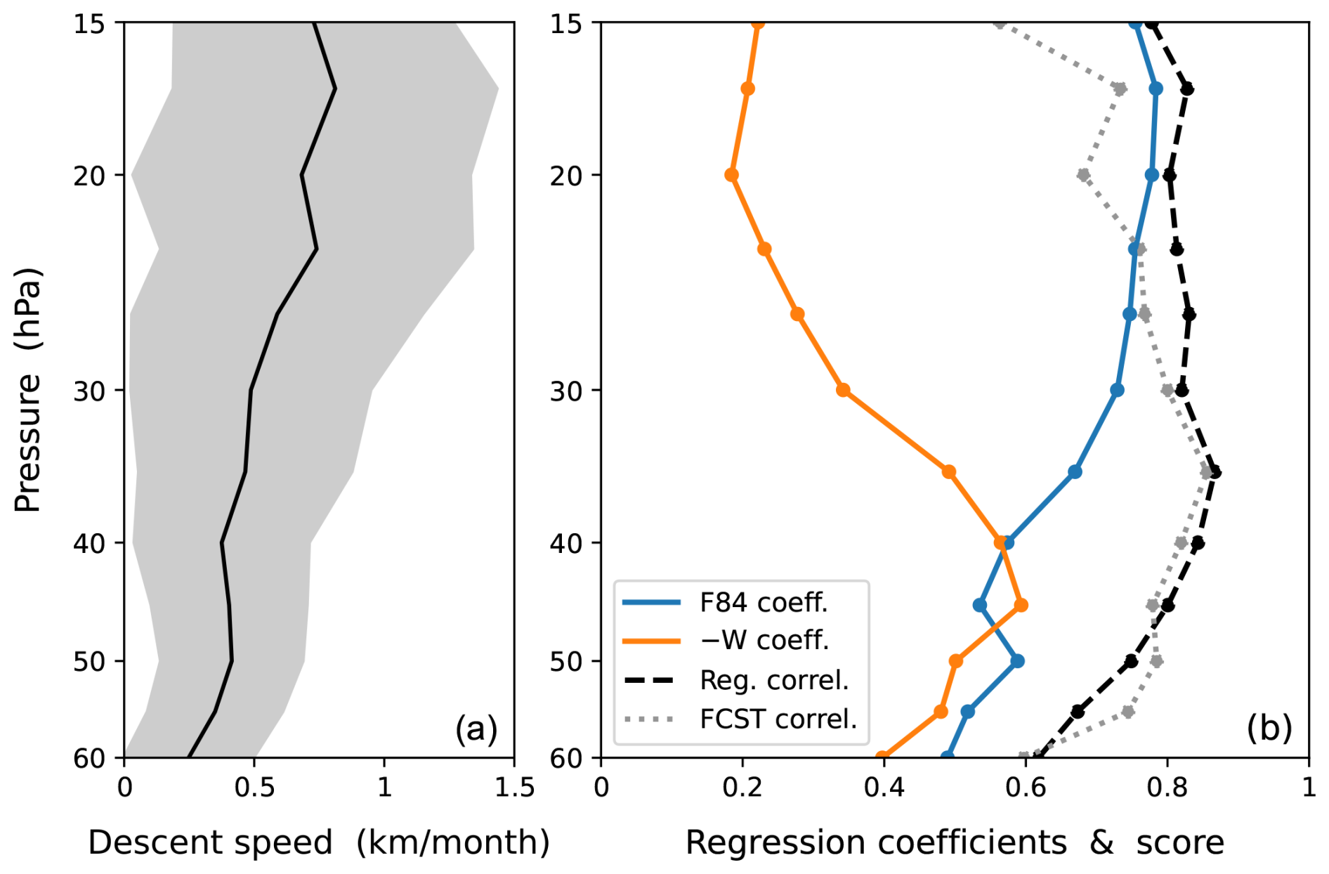
Figure 3 (a) Climatological mean (black line) and variation within 1 standard deviation (gray shading) of the descent speed of the easterly QBO phase (measured following the vertical trajectory of the −10 m s⁻¹ wind phase in easterly shear) throughout 1956–2015. (b) Standardized regression coefficients of 84 hPa small-scale westward-wave momentum flux (blue line) and stratospheric upwelling (orange line) for the descent speed at each altitude, along with the regression correlation score (dashed black line) (see the text for details of the regression). The dotted gray line in (b) depicts the correlation score of a hindcast using the obtained coefficients and the seasonal cycle of momentum flux and upwelling.

Utilizing the obtained regression coefficients, a hindcast is performed using the climatological-mean (1956–2015) annual cycle of F₈₄ and −W as input. The correlation between the hindcasted and observed descent speeds (Fig. 3b, dotted gray line) is very close to the regression correlation. This result indicates that the seasonal variation in wave flux and upwelling accounts for a large portion of the fluctuations in the descent speed of the easterly phase.

To examine the seasonal variation, we present the descent speeds at 20, 30, 40, and 50 hPa as a function of calendar month in Fig. 5, along with F₈₄ and W at the corresponding time, i.e., when the easterly phase of U_φ descents through each altitude (note that an inverted axis is used for W). Individual monthly values (dots) and their averages for each calendar month (solid lines) are plotted. Additionally, the climatological-mean annual cycles of F₈₄ and W, obtained from the full time series regardless of QBO phase, are superimposed (dashed lines).

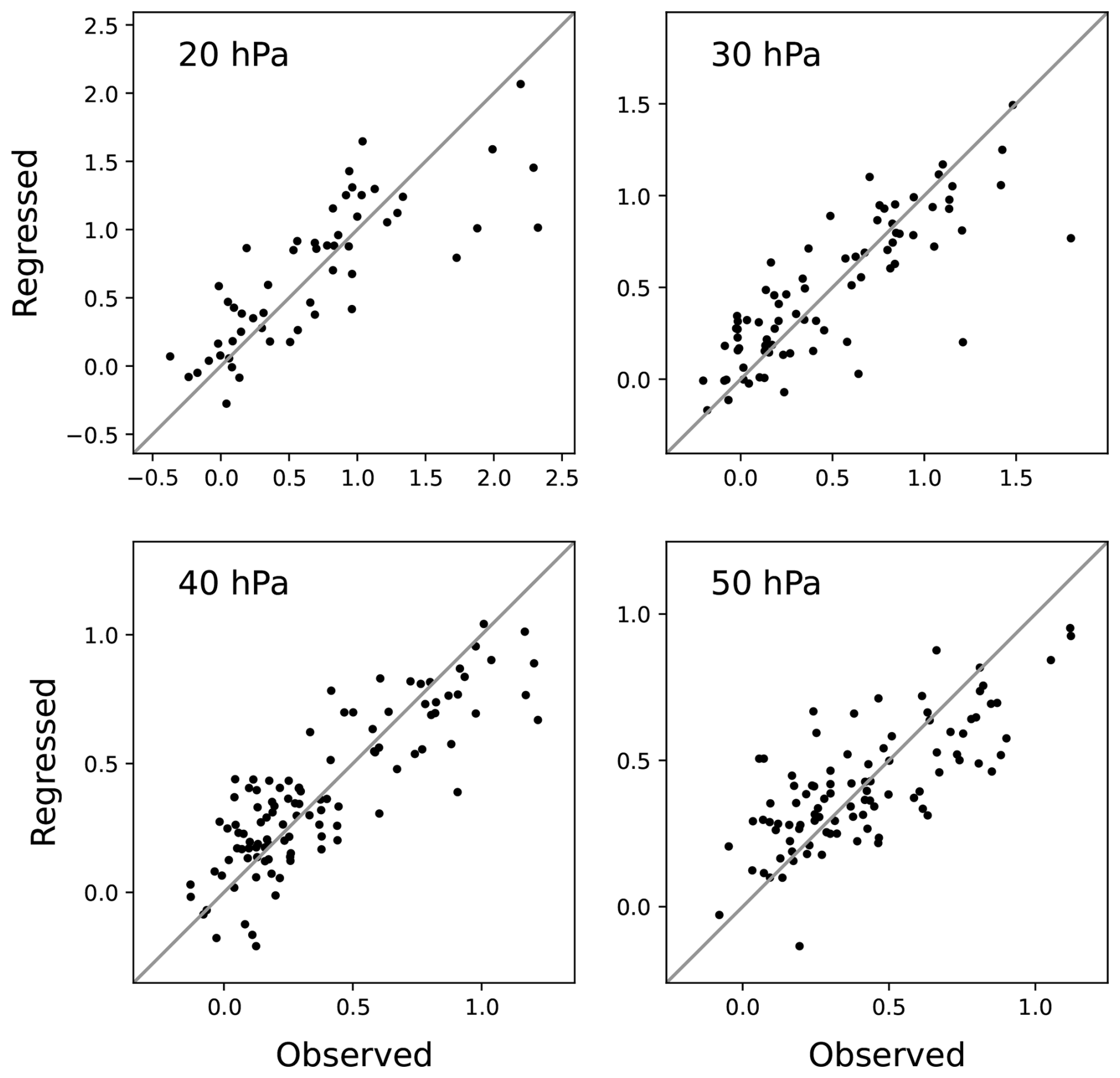
Figure 4 Scatter plots of observed vs. regressed speeds of the easterly-phase descent (in km per month) at 20, 30, 40, and 50 hPa altitudes.

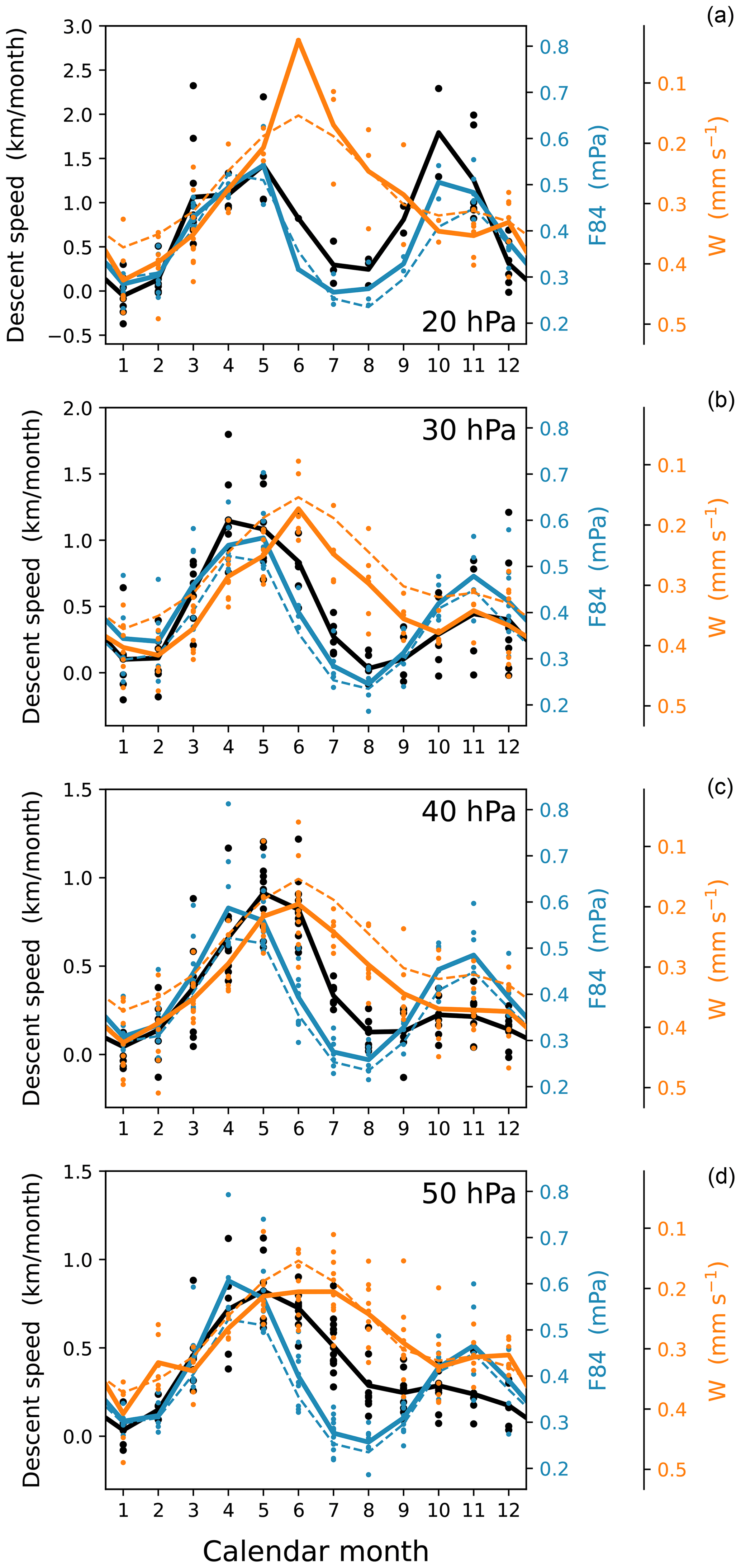
Figure 5 Phase-descent speed (black dots), 84 hPa small-scale westward-wave momentum flux (blue dots), and stratospheric upwelling (orange dots, with an inverted axis) as a function of calendar month, during the easterly-descending phases at 20, 30, 40, and 50 hPa (from top to bottom) throughout 1956–2015. Solid lines indicate their averages for each calendar month. Climatological-mean annual cycles of the wave flux and upwelling, derived from the full time series regardless of QBO phase, are additionally plotted in all panels (dashed lines).

The descent speed (solid black line) exhibits a semiannual variation at 20 hPa, with maxima in April–May and October–November. Compared to the former maximum, the latter weakens with decreasing altitude, becoming almost extinct at 50 hPa. Notably, the descent speed is nearly zero around January and August at 20–40 hPa, indicating the stalling of the phase descent. At 50 hPa, the descent speed is generally low throughout the period from August–February, while the stalling occurs mainly in January (also see Fig. 1a). The seasonal variation in descent speed shown in Fig. 5 is broadly consistent with previous studies (e.g., Wallace et al., 1993, Fig. 13; Coy et al., 2020, Fig. 1).

The annual cycles of F₈₄ and W derived for the easterly-descending phases (solid blue and orange lines, respectively) show similar variations to their climatological-mean cycles (dashed lines) at all altitudes (Fig. 5). F₈₄ exhibits a semiannual variation, whereas W is dominated by an annual variation, resulting in their linear independence to a reasonable approximation (with a correlation of −0.11 between the climatological cycles). Figure 5 indicates that the descent speed variation at 20–30 hPa primarily follows the variation in F₈₄. However, the influence of W variability increases with decreasing altitude. At 40–50 hPa, the descent speed variation appears to be explained only when both variables are collectively considered. This seasonal-cycle analysis supports the regression results shown in Fig. 3b.

Additionally, individual values of F₈₄, W, and descent speed show substantial spread within each calendar month. These variations, on interannual or longer timescales, may not have been successfully modeled in the regression, thereby limiting the regression score to ∼0.8 (Fig. 3b). This is inferred from the fact that the hindcast using the climatological annual cycle yields a similar correlation score. Further investigation of these longer-term variations is left for future studies, while the remaining sections concentrate on seasonal variation.

4.2 Temporal variations in momentum forcing

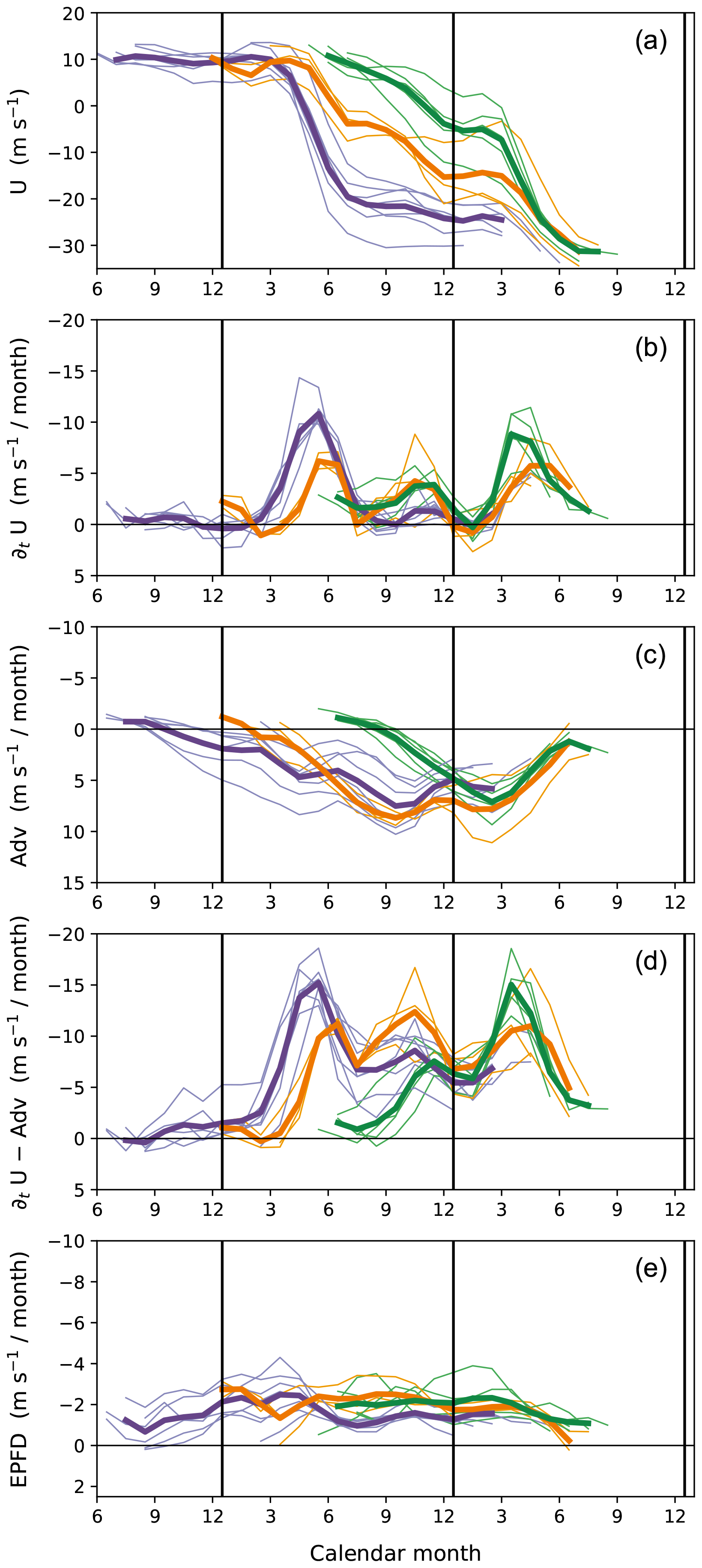
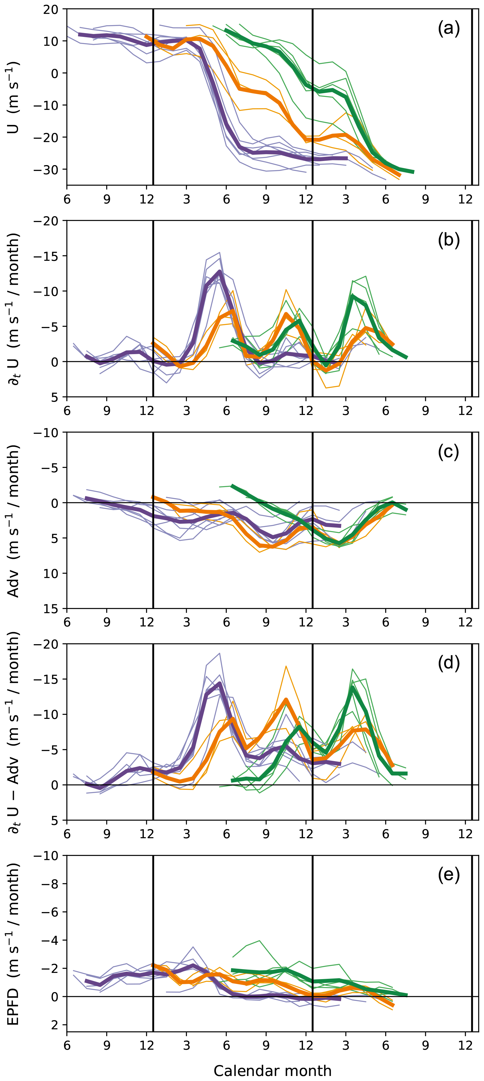
The time evolutions of wind and associated momentum forcing at fixed altitudes are analyzed to investigate the temporal variations of phase-progression speed. Figure 6a and b show the time series of winds at 30 hPa (a middle level of the vertical QBO span) and their change rates, respectively, during the westerly–easterly transition phase in every QBO cycle in 1956–2015 (thin lines), as a function of calendar month. In all cycles, the phase progression occurs only during certain months: March–July and September–December, consistent with previous studies (e.g., Schenzinger et al., 2017). Accordingly, the cycles can be divided into three groups based on the pattern of phase progression. The first group (purple lines in Fig. 6) consists of cycles in which the phase change occurs essentially during March–July. The second group (green lines) includes cycles where the phase changes first to a weak easterly during September–December, stagnates until the following February, and then changes further in March–July. The third group (orange lines) experiences the first phase change in March–July and the final change in the next March–July. (See Appendix A for the categorization procedure.) The thick lines in Fig. 6 represent the averaged time series for each group. Note that the stagnation of phase over time at a given altitude results in the stalling of phase descent (see Fig. 1a; Fig. 5, black line).

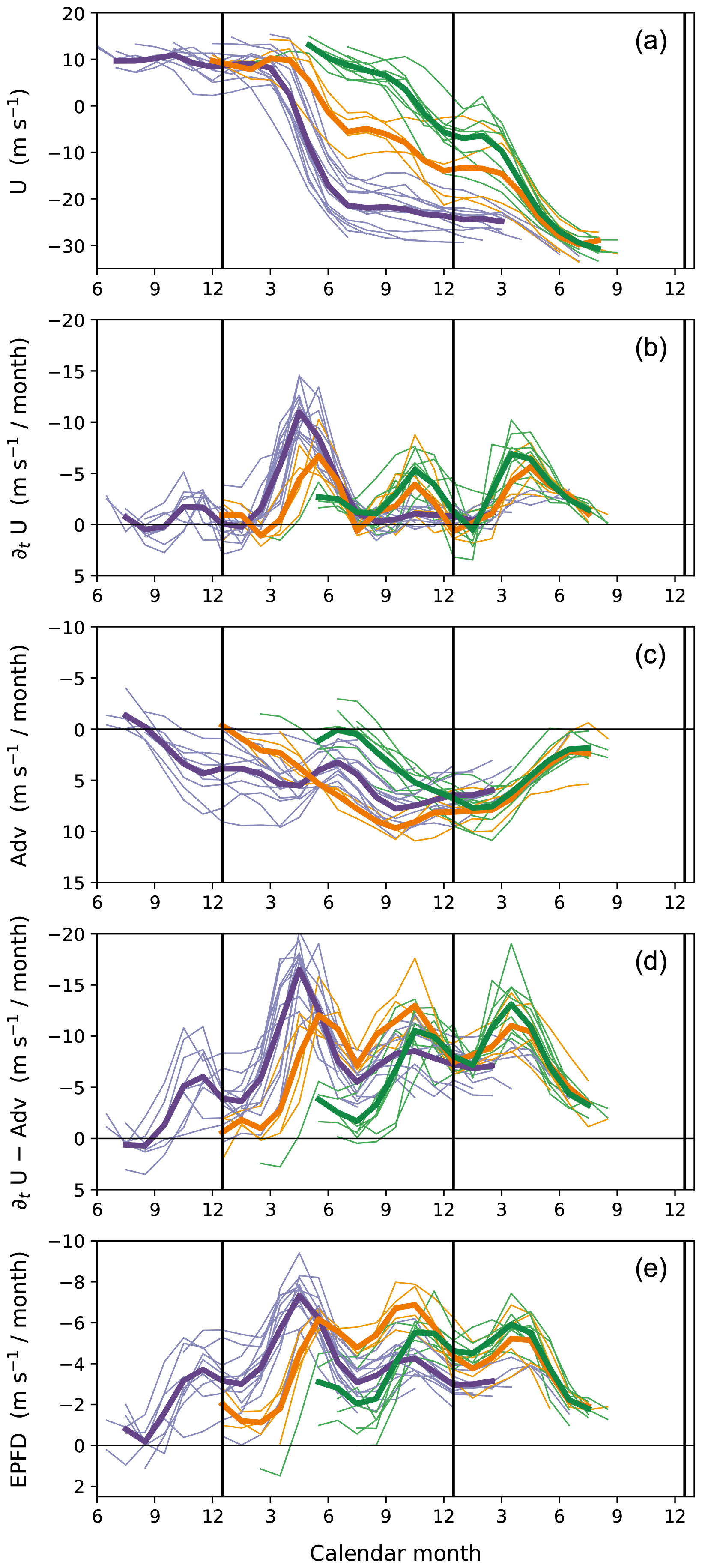
Figure 6 Time series at 30 hPa from the westerly maximum to the easterly maximum phase in each cycle of the QBO during 1956–2015 (thin lines), showing (a) the zonal wind over 5° N–5° S, (b) its tendency, (c) the sum of advection and Coriolis force (Adv), (d) the tendency with the contribution of Adv subtracted (i.e., b minus c), and (e) the Eliassen–Palm flux divergence (see Eq. 1), as a function of calendar month. The cycles are divided into three groups (indicated by different colors) based on the pattern of phase progression (see the text), and the averages for each group are plotted by thick lines. Note that the y axes in (b)–(d) use the same scale interval, and the scale in (e) is half that.

Figure 6c presents the contribution of meridional circulation $({\stackrel{\mathrm{‾}}{v}}^{*},{\stackrel{\mathrm{‾}}{w}}^{*})$ to the wind tendencies (i.e., sum of the vertical and meridional advection and the Coriolis force in Eq. 1) at 30 hPa. In general, they have the opposite sign to the observed wind tendencies (cf. Fig. 6b), implying the retarding effect of the upwelling on the phase evolution. However, they show rather slow temporal variations that are not coherent with those of the observed tendencies for each group of cycles. For quantitative comparison, Fig. 6d shows the portion of the wind tendencies with the contribution of meridional circulation subtracted (i.e., the tendencies minus all terms except the EP flux divergence in Eq. 1). These time series still exhibit large monthly variations similar to the observed tendencies (Fig. 6b), with the two peaks in March–July and September–December, respectively. Note that, given the momentum budget (Eq. 1), the time series shown in Fig. 6d are regarded as an indirect estimate of the total wave forcing, up to potential errors in the circulation contribution calculated from the reanalysis data.

The direct estimate of the wave forcing, as resolved in the reanalysis field (i.e., the explicitly calculated EP flux divergence), is presented in Fig. 6e. Its time series exhibit very similar temporal variations to the indirect estimate of the forcing (Fig. 6d) throughout the phase evolution: both estimates of the forcing start increasing in the early phase when the flow is westerly for each group (Fig. 6d, e, and a), and afterward, they manifest the two peaks in annual variation. The forcing tends to weaken once the flow becomes strongly easterly. The temporal variations in the indirect estimate (Fig. 6d) suggest that the variability in wave forcing is the main driver of the observed (semi)annual behaviors of phase progression and stagnation at 30 hPa shown in Fig. 6a and b; this is ultimately confirmed by the agreement of the explicitly calculated EP flux divergence (Fig. 6e). However, it should be noted that the magnitudes of the direct estimate are roughly half those of the indirect estimate (this underestimation was far larger than the error due to the use of vertically truncated fields at conventional pressure levels in flux calculations, which caused an underestimation of EP flux divergence by roughly 20 % in the tropical stratosphere, not shown). The implication of this is discussed in Sect. 6.

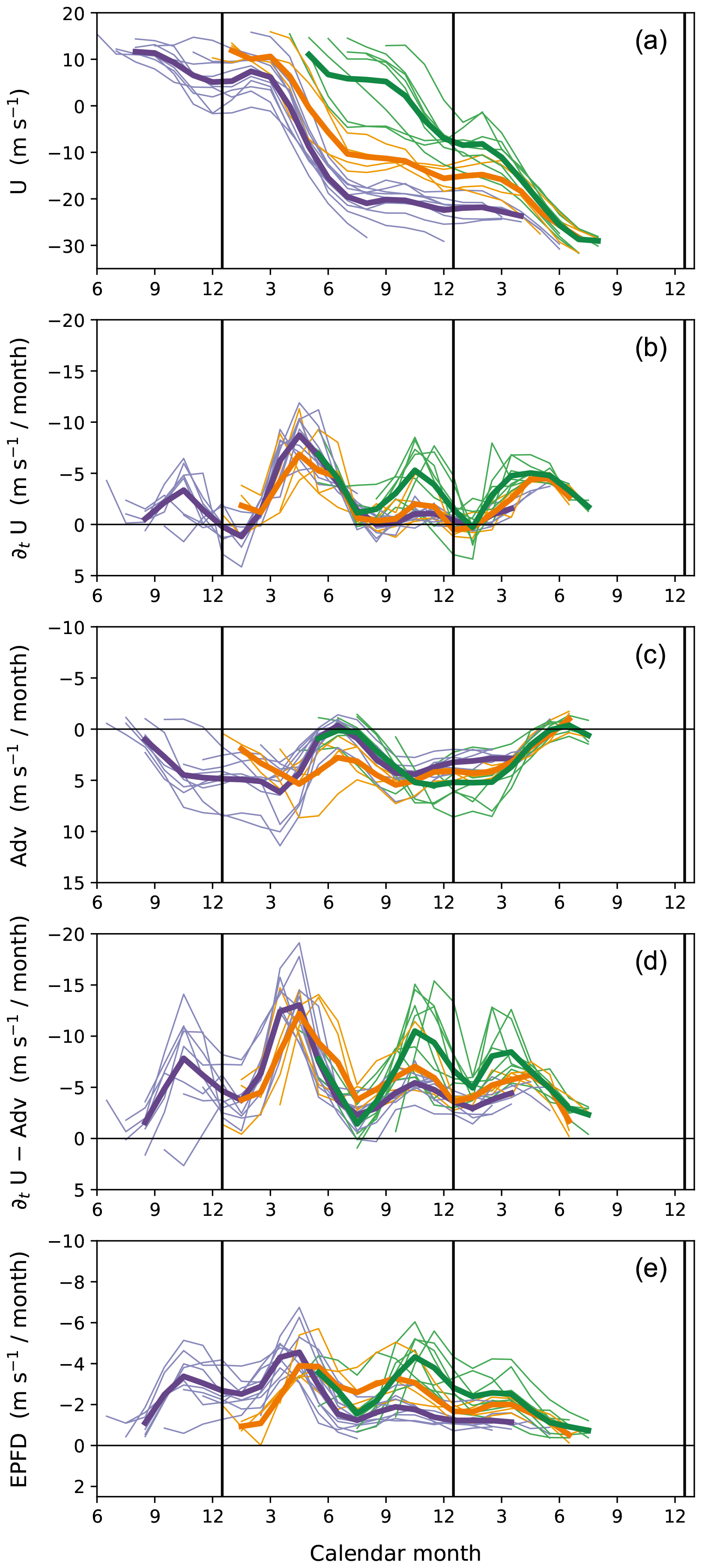
Qualitatively similar results are obtained at other altitudes as well. Figures 7 and 8 present the same analysis as Fig. 6 except at 20 and 50 hPa, respectively. Common to all altitudes, the westerly–easterly phase progression occurs during March–July and September–December but stagnates otherwise. In other words, the months in which the phase descent typically stalls do not change with altitude (see also Fig. 5, black lines). This behavior is largely attributed to the variations in wave forcing, as the months of maximum and minimum forcing remain consistent across altitudes (panels labeled e in Figs. 6–8). Note that these months also align with the seasonal variation in flux entering the stratosphere (F₈₄ shown in Fig. 5, dashed blue line), suggesting that the flux variation is responsible for them. (Accounting for more details in the evolution of wave forcing would require considering the phase-speed spectrum of flux along with the QBO shear; see Eq. 2.)

In contrast, the advection term (panels labeled c in Figs. 6–8) does not show consistent seasonal variations between altitudes. This may result from the strong dependence of both local circulation $({\stackrel{\mathrm{‾}}{v}}^{*},{\stackrel{\mathrm{‾}}{w}}^{*})$ and zonal wind shear on the QBO phase. Nonetheless, the advection term also seems to have a seasonal tendency at lower altitudes (e.g., Fig. 8c for 50 hPa), with relatively larger values during the latter half of the year. Across panels labeled b in Figs. 6–8, the semiannual variability in wind tendencies decreases with decreasing altitude, accompanied by slower phase progression during September–December than during March–July. This suppressed phase progression in September–December at lower altitudes may be influenced by the seasonal tendency of the advection term. Another effect of the circulation on the annual variations in phase-progression speed is discussed in the following section.

The coherent variation of the direct wave-forcing estimate (as resolved in the dataset) with the observed wind changes is striking, as this has never been revealed by long-term observational data or reanalyses (cf. for an 11-year satellite-based estimate of wave forcing, see Ern et al., 2014, Fig. 3c). Existing reanalyses, except the two most recent products (ERA5; JRA-3Q, Kosaka et al., 2024), have generally represented little wave forcing with indistinct monthly variations throughout the westerly–easterly transition phase of the QBO (see Appendix B for the results using additional reanalysis datasets including JRA-3Q).

4.3 Momentum forcing contributions to phase descent speed

In Sect. 4.1, variations in the descent speed of the easterly phase were regressed using factors external to the QBO for causal attribution: wave flux entering the stratosphere (F₈₄) and tropical stratospheric mean upwelling (W). This analysis provided contributions of waves and meridional circulation to the descent speed variation, based on their correlations. However, these contributions can also be quantitatively examined using the zonal-momentum forcing locally exerted at the level of phase descent (i.e., the forcing presented in Sect. 4.2 but specifically during the phase descent), as the descent speed is expressed as the wind tendency divided by shear (Eq. 2). Figure 9 shows the phase descent speed at 20, 30, and 50 hPa and the contributions from total wave forcing and circulation $({\stackrel{\mathrm{‾}}{v}}^{*},{\stackrel{\mathrm{‾}}{w}}^{*})$ (namely, the respective zonal forcings in Eq. (1), each divided by shear) as a function of calendar month. For the wave forcing, we primarily use its indirect estimate (which is shown in panels labeled d in Figs. 6–8) for quantitative analysis, due to the underestimation of explicitly calculated EP flux divergence (panels labeled e).

Figure 7 As in Fig. 6 except at 20 hPa.

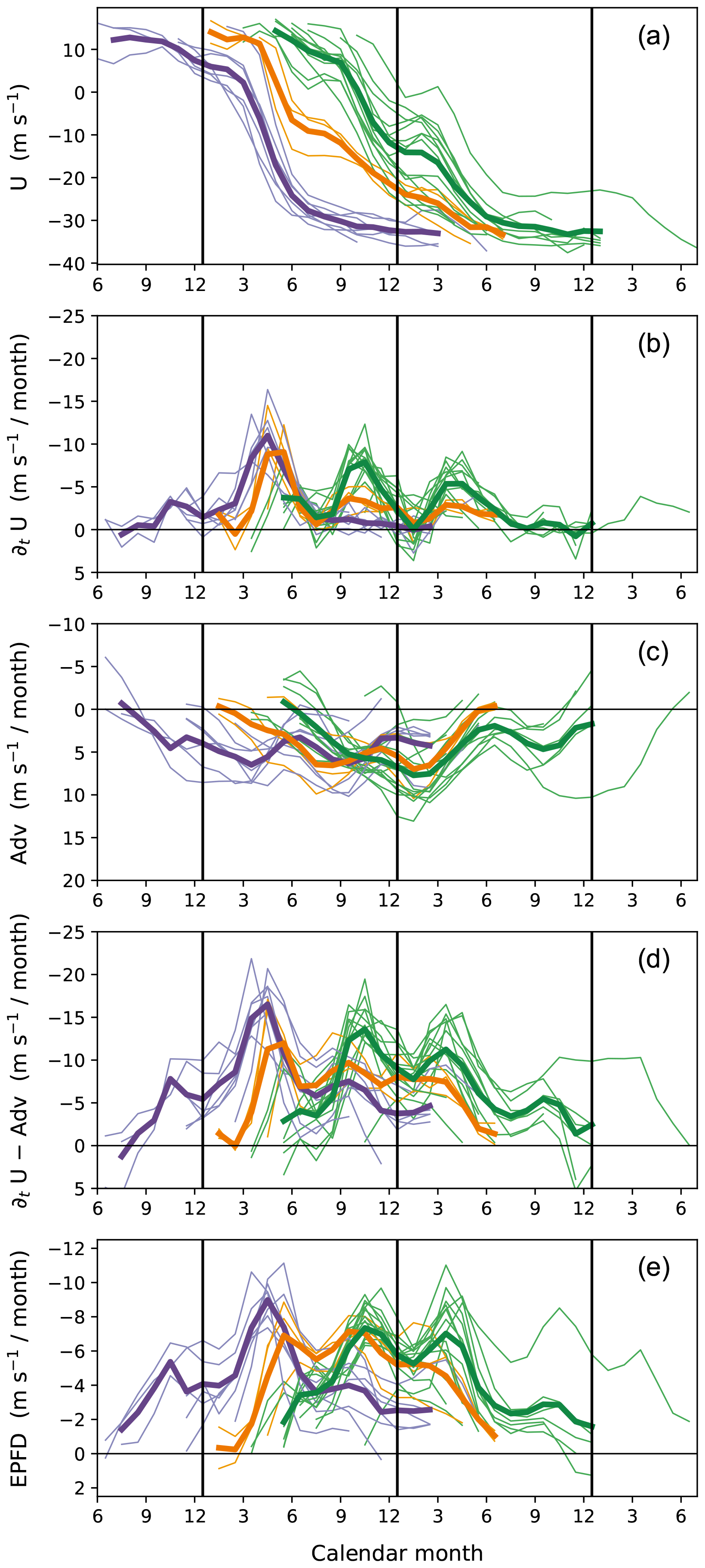
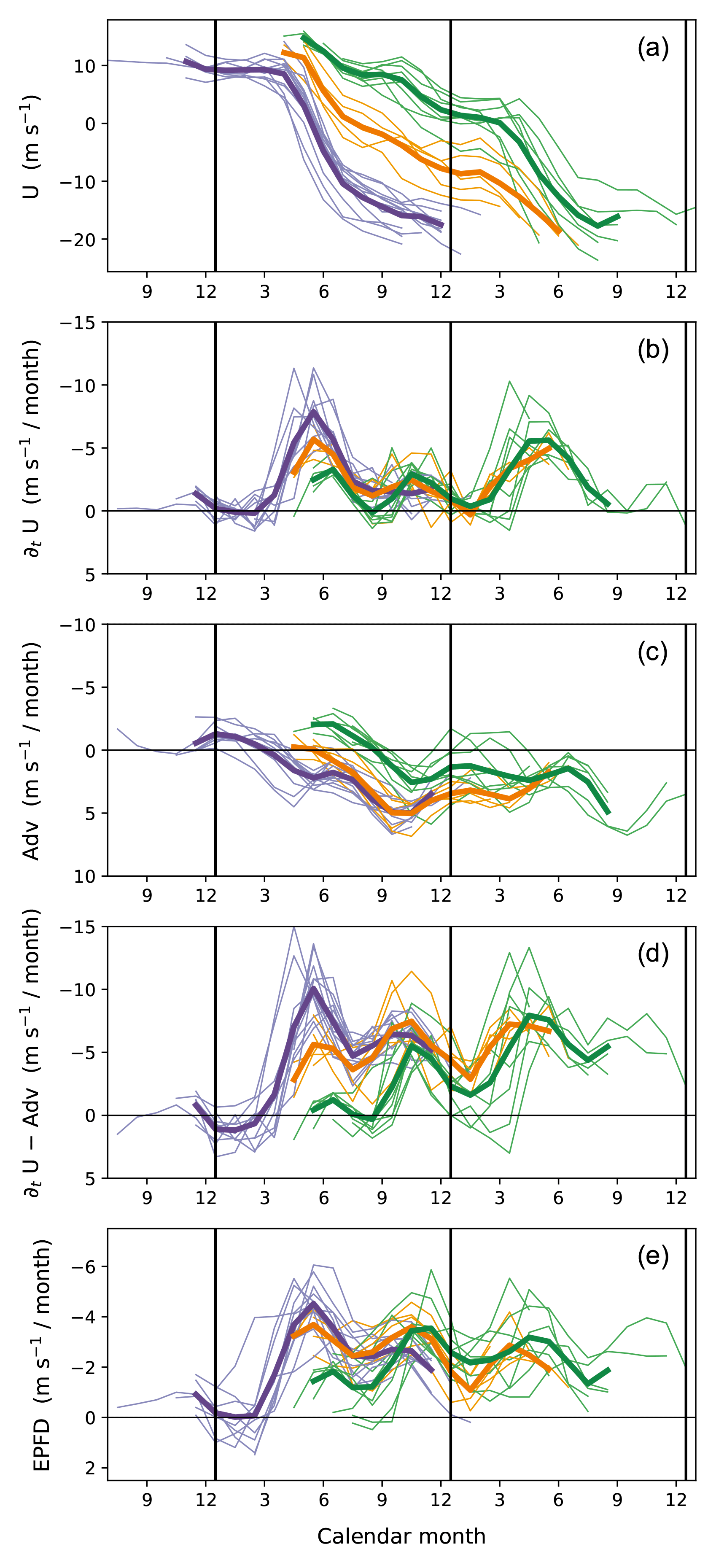
Figure 8 As in Fig. 6 except at 50 hPa. For better visibility, the time series are shown only after the wind at 30 hPa has transitioned to easterly.

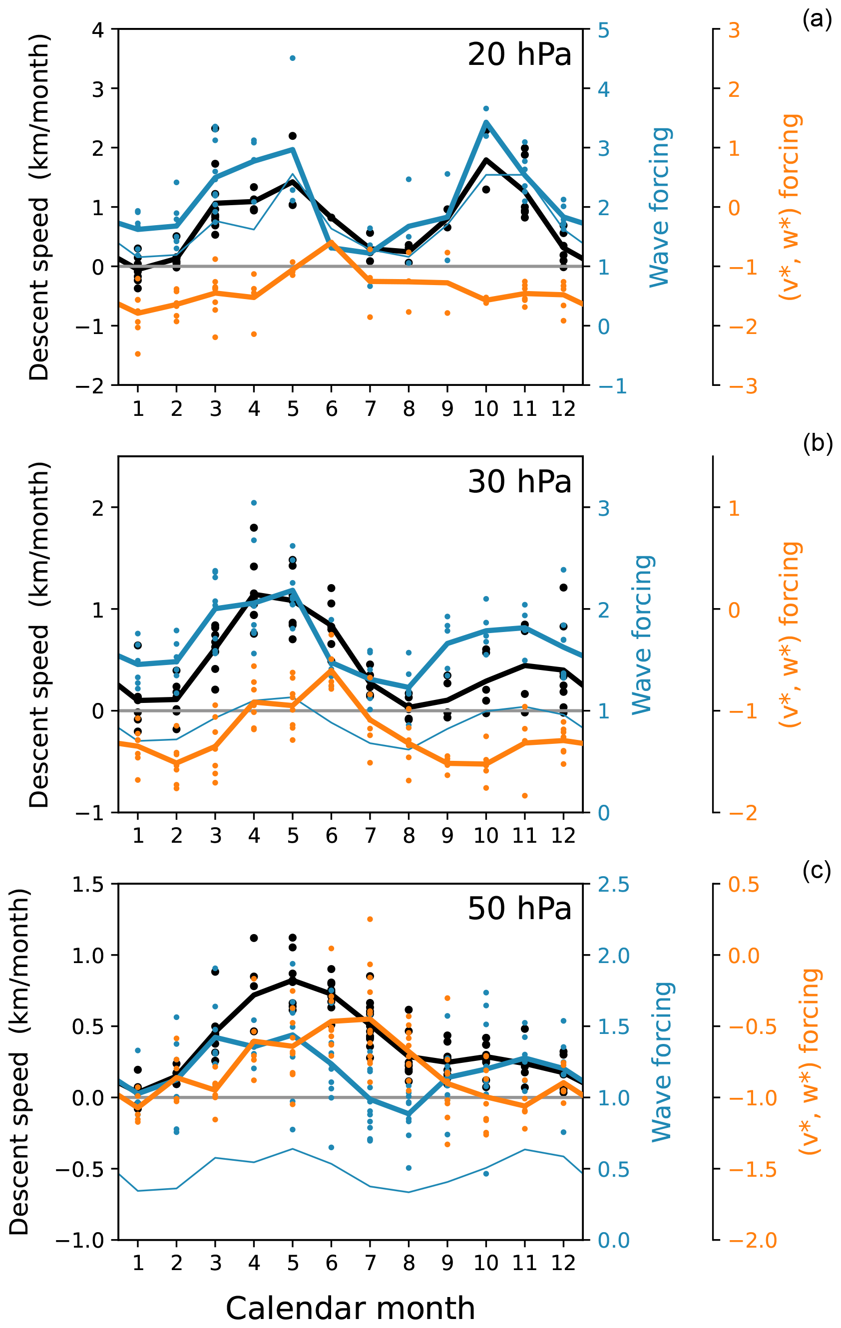
Figure 9 Descent speed of the easterly phase (black dots) at 20, 30, and 50 hPa (from top to bottom) during 1956–2015, along with contributions from meridional-circulation-induced forcing (orange dots) and wave forcing (blue dots), as a function of calendar month. Thick solid lines indicate their averages for each calendar month. The circulation contribution is calculated as the sum of advection and Coriolis force (Adv, Fig. 6c) divided by zonal wind shear, and the wave contribution is calculated as the indirect estimate of total wave forcing (Fig. 6d) divided by the shear, both in the same units as descent speed. The 5° N–5° S averaged forcing and shear are used. Additionally, the wave contribution derived from the Eliassen–Palm flux divergence (Fig. 6e) is plotted but only for the calendar-month average (thin blue line).

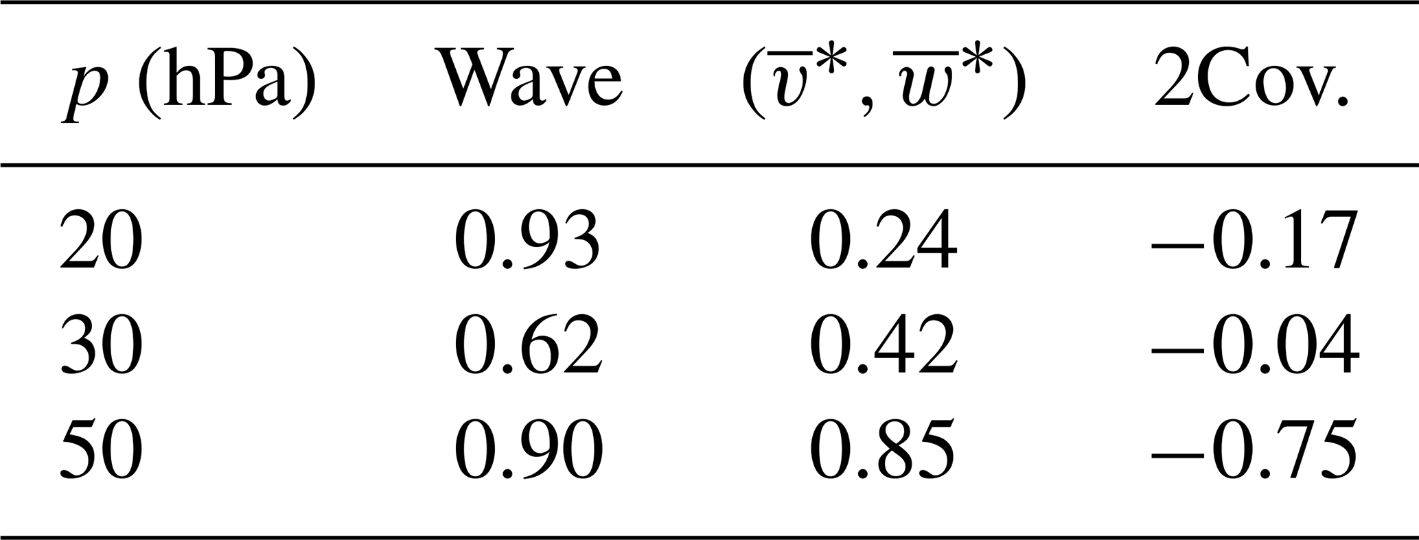
The wave forcing contribution (thick blue lines in Fig. 9) accounts for the majority of variability in descent speed (black lines) at 20 hPa. The contribution of meridional circulation (orange lines) increases with decreasing altitude, showing variability comparable to that of wave forcing at 50 hPa. These results are quantified in Table 1, which presents the relative contributions to the variance of descent speed at each altitude from the wave and circulation forcing, along with the contribution from their covariance. The variance decomposition is based on the following expression:

$${\displaystyle }{\displaystyle }\text{Var}[X_{\mathrm{1}}+X_{\mathrm{2}}]=\text{Var}\left[X_{\mathrm{1}}\right]+\text{Var}\left[X_{\mathrm{2}}\right]+\mathrm{2}\text{Cov}[X_{\mathrm{1}},X_{\mathrm{2}}],$$

where X₁ and X₂ are the respective forcings divided by wind shear (blue and orange dots in Fig. 9). These results are generally consistent with the findings from the regression (Figs. 3b and 5), although $({\stackrel{\mathrm{‾}}{v}}^{*},{\stackrel{\mathrm{‾}}{w}}^{*})$ here includes the local circulation induced by the QBO, and its associated forcing is largely correlated with the wave forcing at 50 hPa (Table 1; cf. Sect. 4.1). The wave forcing contribution derived from the explicitly calculated EP flux divergence (thin blue lines in Fig. 9) exhibits similar seasonal variations to those from the indirect estimate, although its magnitude is underestimated by up to ∼50 %.

It should be noted that the wave forcing examined here includes contributions from all scales, encompassing wavelengths greater than 2000 km. Although we did not decompose the wave forcing by scale, we assume that small-scale waves dominate the total wave forcing and its seasonal variation during the descending easterly phase. This may be supported by previous findings that earlier reanalysis products, which are expected to resolve large-scale waves, show only limited magnitudes of westward wave forcing (e.g., Ern et al., 2014; Kim and Chun, 2015b). Figures B1e and B2e further reveal that its seasonal variation is also limited.

Table 1 Relative contributions to the variance of descent speed from wave forcing, circulation forcing, and their covariance.

5 Seasonal modulation of wave activity

The monthly variations in wave momentum flux and forcing examined in Sect. 4 are explained by the seasonal cycle of tropical convective activity and that of the wind in the tropopause layer, which both modulate the wave flux into the stratosphere. Figure 10a presents the climatological annual cycle of the upward flux of westward momentum due to the small-scale waves at 200 hPa (∼12 km) altitude. In the upper troposphere, the spatio-temporal variation of the wave momentum flux generally follows the seasonal cycle of precipitation (white contours in Fig. 10a), which is a proxy for convective activity as the source of waves.

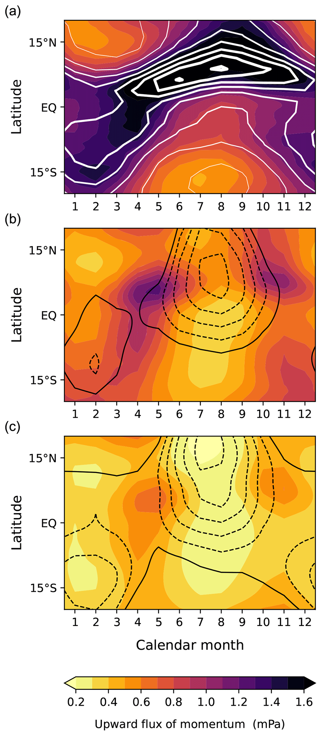
Figure 10 Climatological-mean annual cycle of upward flux of westward momentum due to waves with zonal wavelengths less than 2000 km (shading) at (a) 200 hPa, (b) 125 hPa, and (c) 84 hPa. The GPCP monthly precipitation rate is superimposed in (a) (white contours at intervals of 1 mm d⁻¹). In (b) and (c), the vertical minima of zonal wind in the 125–200 hPa layer and the 84–200 hPa layer, respectively, are superimposed (solid black contours for zero winds; dashed black contours for easterlies at intervals of 3 m s⁻¹).

However, the monthly variation of the flux is significantly altered in the tropopause layer, as shown at 125 hPa (∼15 km, Fig. 10b). The 125 hPa flux exhibits two peaks, April–May and October–November, while the overall flux magnitude is reduced compared to that at 200 hPa. It is because of the dissipation of wave momentum flux by the flow in the 200–125 hPa layer, which occurs more severely under the easterly condition for the flux of westward momentum due to gravity waves propagating westward. The flow in this layer (black contours in Fig. 10b) is easterly in the summer hemisphere. This condition, along with the weak convective activity in the winter hemisphere (Fig. 10a), results in relatively small fluxes during both solstices, with maxima occurring in April–May and October–November. A qualitatively similar monthly variation of the flux was previously obtained by Kim and Chun (2015a, Fig. 6) using a parameterization of convective gravity waves in a climate model, which supports the role of convection and tropopause layer wind in the flux variation.

The flux at 84 hPa (Fig. 10c) shows a similar variation to that at 125 hPa with the same months of maxima, while being further dissipated in between. The pattern of seasonal variation does not change significantly with latitude over 15° N–15° S. For the flux averaged over this latitude band (i.e., F₈₄ in the climatological mean shown in Fig. 5, dashed blue line), the maxima are approximately 0.52 mPa in April–May and 0.45 mPa in October–November, while the minima are about 0.30 mPa in January and 0.24 mPa in August. As noted in the regression analysis in Sect. 4.1, a large portion of the fluctuations in the descent speed of the easterly phase is explained by this flux variation, even when only its climatological seasonal cycle is considered (Fig. 3b, dotted gray line). Notably, while the above-mentioned flux variation (0.24–0.52 mPa) corresponds to ±37 % of its annual mean, it leads to an even larger variation in the phase descent speed (about ±50 % at all altitudes, Fig. 5, black lines) because upwelling reduces the descent speed on average (see Eq. 2). This upwelling effect in amplifying the response of descent speed to the flux variations occurs regardless of the seasonal variability in upwelling. This is in addition to the direct effect of upwelling variability on the descent speed at low altitudes (p≳40 hPa), discussed in Sect. 4.1.

In contrast to this westward momentum flux, the eastward momentum flux due to small-scale waves exhibits a smaller annual variation at 84 hPa (ranging from 0.42 to 0.52 mPa) when averaged latitudinally, although it has strong seasonality in its latitudinal distribution (see Fig. C1). Even when larger-scale waves, such as Kelvin waves, are considered collectively, the annual variation in total eastward momentum flux (not shown) remains within ±15 % of its annual mean (∼1.25 mPa). The relatively constant speed of the westerly-phase descent within each QBO cycle, discussed in Sect. 3 (Fig. 1a), may be attributed to the smaller annual variation in eastward momentum flux. Furthermore, where the westerly phase descends, the upwelling velocity is minimal due to the QBO-induced local circulation and therefore does not significantly affect the phase-descent speed or its variation, unlike in the opposite phase. However, a more detailed investigation may be necessary to fully explain this phase, as the dissipation mechanism of Kelvin waves differs from that of small-scale gravity waves (e.g., Ern et al., 2009; Krismer and Giorgetta, 2014). In addition, the QBO-westerly amplitude is relatively small (∼15 m s⁻¹), implying that only a part of the wave spectrum contributes to the westerly-phase descent.

6 Summary and discussions

We revealed that the QBO period fluctuates primarily due to the temporal variation in the amount of westward momentum carried by small-scale waves (gravity waves). The speed of the easterly-phase descent, the key factor controlling the QBO period, was highly correlated with the gravity-wave momentum flux estimated in the tropical tropopause layer. Furthermore, the stratospheric momentum forcing exerted by the waves demonstrated coherent variations with the observed phase evolutions of the QBO. The annual variation of the wave momentum flux was explained by the seasonal cycles of tropical convection and tropopause layer wind. Other sources of variation, such as the El Niño–Southern Oscillation (ENSO) (Taguchi, 2010) and volcanic eruptions (DallaSanta et al., 2021), may also be involved on longer timescales. However, it is notable that the annual variation already accounts for the typical behaviors of phase progression and stagnation in observed QBO cycles. The contribution of variability in stratospheric upwelling to the fluctuation of the QBO descent speed was found to be relatively minor above ∼40 hPa altitude but became comparable to the wave contribution below that level.

Although the primary target for atmospheric reanalysis products may have been to resolve synoptic-scale weather systems and embedded larger-scale circulations, their resolutions are continuously improving beyond these scales. Our study demonstrates that waves with horizontal wavelengths less than ∼2000 km play a crucial role in QBO period fluctuations. It is encouraging that the reanalysis used here represents the interaction between these small-scale waves, convection, and the mean-flow oscillation with realistic variations, implying more opportunities for studies on multiscale atmospheric phenomena beyond the synoptic scale. However, we also note that scales smaller than a few hundred kilometers are still largely truncated in current-generation reanalyses, including the one used here. This limitation may have led to an underestimation of the wave flux and forcing presented in our results (compare Fig. 6d to e), suggesting that the actual impact of small-scale waves could be even more significant than our analysis indicated. In addition, although our analysis captured the temporal variations in small-scale wave activity that are highly correlated with the QBO phase speed, this does not necessarily imply that the detailed representation of convective gravity waves in the reanalysis is fully realistic, particularly when examined for individual events of convection and waves. Addressing these limitations, a comprehensive understanding of the processes, including full variability of the waves, remains essential for gaining deeper insight into the QBO.

Beyond the advancement in our understanding of QBO dynamics, these findings have important implications for both seasonal predictions and long-term climate projections. They suggest that prediction models should accurately represent the coupled variability of convection, small-scale waves, and the mean flow to improve seasonal forecasts of the QBO and related atmospheric teleconnections. This precise representation is also crucial for future climate projections of the QBO, which have shown a large spread between climate models (Butchart et al., 2020; Richter et al., 2022). By better capturing these multiscale interactions, models may provide more reliable projections of future QBO behavior and its impacts on global climate.

Appendix A: Procedure for QBO-cycle categorization

The categorization of cycles with respect to the pattern of westerly–easterly phase evolutions in Figs. 6–8 was motivated by their distinction into three groups as described in Sect. 4.2. For objective categorization, we used two criteria: the calendar month when the wind substantially weakened to less than U₁ and how the wind changed over the subsequent 5 months (U₂). With U₁=0 (except at 50 hPa, where it was set to 5 m s⁻¹), the QBO cycles in which the wind changed below U₁ in January–July were categorized into the first or second groups (purple and green lines, respectively, in Figs. 6–8); the other cycles were categorized into the third group (orange lines). The first group was separated from the second by fast phase evolution with $U_{\mathrm{2}}<-\mathrm{20}$, −15, and −8 m s⁻¹ at 20, 30, and 50 hPa, respectively. The altitude dependence of U₁ and U₂ values was due to the vertical change in QBO amplitude.

At 30 hPa (Fig. 6), some cycles in the first and third groups (purple and orange lines, respectively) appear to exhibit a similar wind phase of 10 m s⁻¹ around March, just before undergoing distinct phase evolutions. The distinct evolutions from the similar wind phase are attributed to the larger vertical shear in the first group compared to the third, which results from differences in QBO phases at higher altitudes between the groups (not shown). The larger shear induces stronger wave forcing (Fig. 6d and e) as explained in Sect. 4.1, leading to earlier phase changes in the first group.

Appendix B: Results from other reanalysis datasets

Three additional reanalysis products were used for comparison: the ECMWF Interim Reanalysis (ERA-Interim, Dee et al., 2011a); the Modern-Era Retrospective Analysis for Research and Applications, version 2 (MERRA-2, Gelaro et al., 2017); and the Japanese Reanalysis for Three Quarters of a Century (JRA-3Q, Kosaka et al., 2024). ERA-Interim has a horizontal resolution of ∼80 km, starting from 1979; MERRA-2 offers a resolution of ∼50 km, starting from 1980; and JRA-3Q has a resolution of ∼40 km, from September 1947. However, we excluded data prior to 1963 due to its unrealistic representation of the QBO winds during that period.

Figure B1 As in Fig. 6 except using ERA-Interim for the period of 1980–2015.

Figure B2 As in Fig. 6 except using MERRA-2 for the period of 1980–2015.

Figure B3 As in Fig. 6 except using JRA-3Q for the period of 1963–2015.

Figures B1 and B2 show the evolutions of 30 hPa winds, tendencies, and momentum forcing during the westerly–easterly transition phase, as in Fig. 6 but using ERA-Interim and MERRA-2, respectively, during the period of 1980–2015. All the terms, except the EP flux divergence, exhibit qualitatively similar results to those using ERA5 (Fig. 6). However, the EP flux divergence obtained from these datasets is generally much smaller than that using ERA5, with indistinct temporal variations.

Figure B3 presents the results obtained using JRA-3Q for the period 1963–2015. The EP flux divergence exhibits notable variability, with two annual peaks that are qualitatively similar to those discussed in ERA5 (Fig. 6) but have smaller magnitudes. Overall, the magnitude of the EP flux divergence is roughly one-third of the indirect estimate of wave forcing in JRA-3Q (Fig. B3d and e).

Appendix C: Eastward-wave momentum flux

While this study focuses on westward momentum fluxes due to westward propagating waves, which are responsible for the descent of the easterly QBO phase, eastward momentum fluxes from eastward propagating waves are also presented here for completeness. Figure C1 corresponds to Fig. 10, with the directions of momentum fluxes and zonal wind reversed. The eastward momentum fluxes tend to maintain their seasonal variation from 200 to 84 hPa, as the westerlies are weak in the regions where the fluxes are concentrated (i.e., regions of high precipitation), thus having less impact on them.

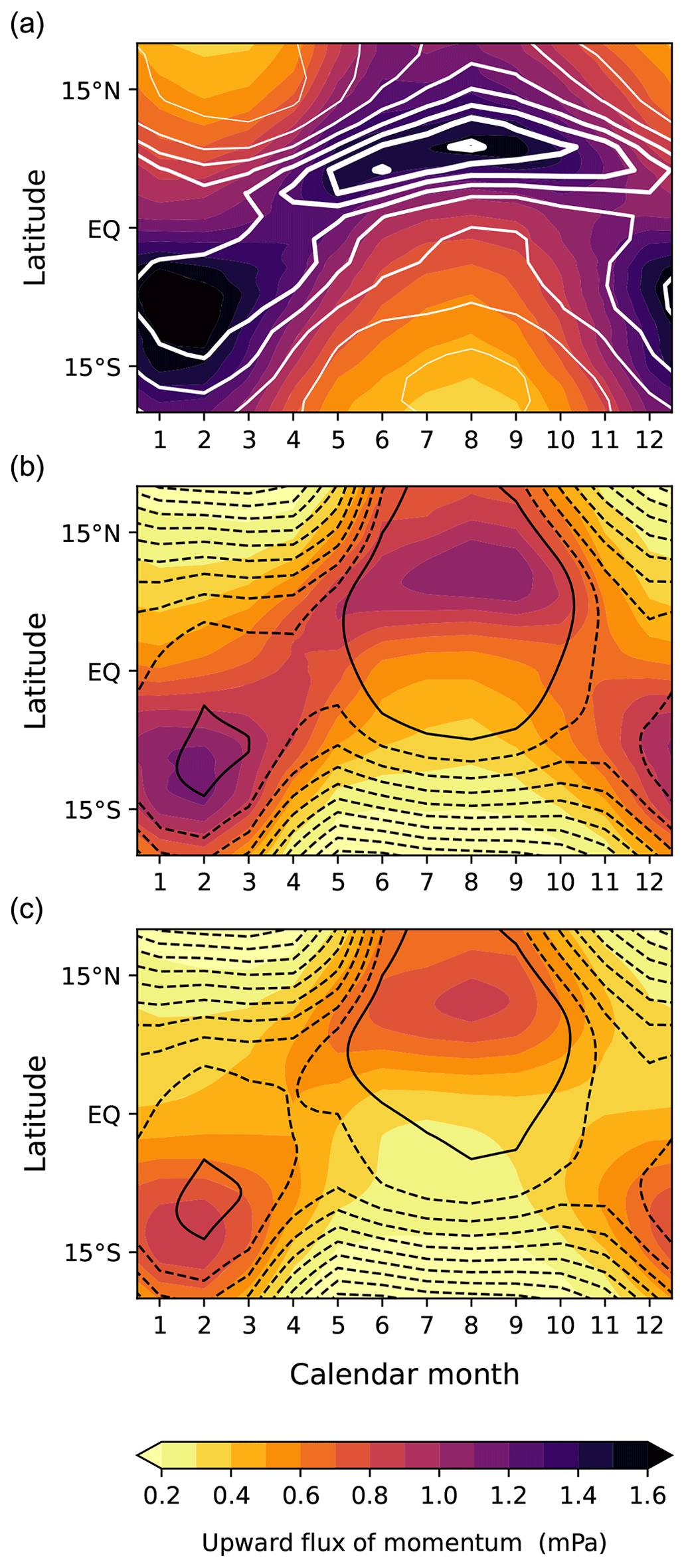
Figure C1 Climatological-mean annual cycle of upward flux of eastward momentum due to waves with zonal wavelengths less than 2000 km (shading) at (a) 200 hPa, (b) 125 hPa, and (c) 84 hPa. The GPCP monthly precipitation rate is superimposed in (a) (white contours at intervals of 1 mm d⁻¹). In (b) and (c), the vertical maxima of zonal wind in the 125–200 hPa layer and the 84–200 hPa layer, respectively, are superimposed (solid black contours for zero winds; dashed black contours for westerlies at intervals of 3 m s⁻¹).