How to trace the origins of short-lived atmospheric species: an Arctic example

The origins of particles and trace gases involved in the rapidly changing polar climates remain unclear, limiting the reliability of climate models. This is especially true for particles involved in aerosol–cloud interactions with polar clouds. As detailed chemical fingerprinting measurements are difficult and expensive in polar regions, backward modeling is often used to identify the sources of observed atmospheric compounds. However, the accuracy of these methods is not well quantified. This study provides an evaluation of these analysis protocols by combining backward trajectories from the FLEXible PARTicle dispersion model (FLEXPART) with simulations of tracers from the Weather Research and Forecast model including Chemistry (WRF-Chem). Knowing the exact modeled tracer emission sources in WRF-Chem enables a precise quantification of the source detection accuracy. The results show that direct interpretation of backward model outputs or more advanced analyses like potential source contribution functions (PSCFs) are often unreliable in identifying emission sources. After exploring parameter sensitivities thanks to our simulation framework, we present an updated and rigorously evaluated backward-modeling analysis protocol for tracing the origins of atmospheric species from measurement data. Two tests of the improved protocol on actual aerosol data from Arctic campaigns demonstrate its ability to correctly identify known sources of methane sulfonic acid and black carbon. Our results reveal that traditional back-trajectory methods often misidentify emission source regions. Therefore, we recommend using the method described in this study for future efforts to trace the origins of measured atmospheric species.

1 Introduction

The warming rate of the Arctic is almost 4 times higher than the global average rate (Rantanen, 2022). In the austral hemisphere, the Antarctic ice sheet, with its accelerating melting, is a point of concern (Bronselaer et al., 2018). This polar amplified warming is concerning for the entire climate science community due to its possible impacts on the atmospheric and ocean circulations (Serreze and Barry, 2011). Studying the rapidly changing polar climates is therefore a research priority.

Short-lived climate forcers, such as aerosols and ozone, play an important role in global and polar climates (IPCC, 2021). Polar regions are especially sensitive to local forcing (Stuecker et al., 2018), and understanding the origin of short-lived climate forcers in these regions is especially important. Their climate impact is dominated by aerosol–cloud interactions, the effect of aerosols on cloud formation and evolution (Storelvmo, 2017). However, our understanding of aerosol forcing remains especially uncertain because of the complexity of its processes and the scarcity of measurements in the polar regions. Polar clouds could be more sensitive to aerosols than in other regions because clouds are usually more sensitive to aerosols in clean conditions (Carslaw et al., 2013). In addition, aerosol–cloud interactions are even more uncertain in ice-containing clouds, which are predominant in polar regions (Matus and L'Ecuyer, 2017).

Controversies remain in the scientific community regarding the nature and sources of the atmospheric species implicated in these mechanisms. For instance, the origins of particles acting as cloud condensation nuclei (CCN, necessary for liquid-cloud droplet formation) or ice-nucleating particles (INPs, involved in cloud ice formation) are a source of great debate (e.g., Zhao et al., 2024). Because modeling of CCN and INP species is often imprecise or even lacking in climate models (Morrison et al., 2020), improved knowledge of their sources would help to fill the present gaps (Murray et al., 2021). In this context, being able to identify the sources of aerosols relevant for CCN and INPs would be decisive in improving our understanding of their emissions, how to represent them in models, and how to quantify their impacts on polar clouds and climate.

In order to identify the origin of observed species, observational studies often rely on analyzing their detailed chemical composition and physical properties (Freitas et al., 2022; Heutte et al., 2025; Parshintsev and Hyötyläinen, 2015; Shao et al., 2022) or their correlation with chemical tracers like carbon monoxide from biomass burning and fossil fuel combustion (Jiang et al., 2009) or dimethyl sulfide from phytoplankton blooms (Park et al., 2017). These extra measurements are often expensive and not systemically present in measurement campaigns, and their interpretation is hardly straightforward.

Another way to identify the sources of observed species is to use backward modeling in an attempt to track their atmospheric path all the way back to the emission sources. This does not require extra experimental data and has the advantage of costing less than observational methods. For example, this kind of analysis is increasingly being used and presented alongside the analysis of INP observations. Some studies have used straightforward interpretation of single back trajectories (Allen et al., 2021; Hartmann et al., 2020, 2021; Porter et al., 2022; Wex et al., 2019; Yun et al., 2022), while others have performed more advanced analyses like potential source contribution functions (PSCFs) (Irish et al., 2019; Si et al., 2019). Even though the methods used vary from one study to another, the conclusions about the possible emission sources can be interpreted similarly across the community, which could be misleading.

Backward modeling consists of the computation of particle paths backward in time within a fluid. As chemistry transport models (CTMs) give information on the future path of particles or chemical species, a back-trajectory model helps to trace back the fluid parcels that contain the species of interest. For atmospheric studies, many models offer solutions for back-trajectory computation. Among the most used, we find two types of approaches. First, there are trajectory models that use solely the resolved wind fields without turbulence or convection parameterization, like the HYbrid Single-Particle Lagrangian Integrated Trajectory (HYSPLIT) model (Stein et al., 2015) and LAGRANTO (Sprenger and Wernli, 2015). Second, there are the Lagrangian particle dispersion models (LPDMs) like FLEXPART (Pisso et al., 2019), NAME III (Jones et al., 2007), or the Stochastic Time-Inverted Lagrangian Transport (STILT) model (Wen et al., 2012). One should know that HYSPLIT can also be run in dispersion mode. In the following, we will refer to the outputs of the first model category as back trajectories and to dispersion model outputs as potential emission sensitivity (PES). Both model types will be referred to as Lagrangian models.

Four different approaches that use Lagrangian modeling can be cited: (1) inverse modeling methods, (2) ratio methods or potential source contribution functions (PSCFs), (3) concentration-weighted trajectory (CWT) methods, and (4) direct interpretation of single back trajectories or LPDM outputs. Inverse modeling methods (1) have been intensively used and developed since the 2000s, particularly for the retrieval of greenhouse gas emissions (Stohl et al., 2009; Manning et al., 2011; Brunner et al., 2012; Fang et al., 2015). They are more rarely applied to aerosol emission source identification because of the challenges their high temporal and spatial variability represent (Dubovik et al., 2008; Partridge et al., 2011). Furthermore, these methods generally rely on a priori inputs in terms of the emissions, such as satellite observations or existing but imprecise emission inventories. PSCFs (2) (Ashbaugh et al., 1985; Zeng and Hopke, 1989) and CWTs (3) (Hsu et al., 2003) are statistical methods that rely entirely on backward modeling and measurement time series. Because they are both easy to set up, they are intensively used (e.g., Polissar et al., 1999; Hirdman et al., 2010; Irish et al., 2019; Ren et al., 2021). Nevertheless, interpretation of raw back trajectories (4) is still common in the literature (see the references relating to INP studies above) and can lead to spurious conclusions about emission sources.

Fang et al. (2018) evaluated the performance of inverse modeling against CWTs and PSCFs and concluded that the high quantitative power of inverse modeling surpasses the qualitative results of CWTs and PSCFs. Yet, PSCFs and CWTs are computationally low cost and can give useful insights when correctly applied and interpreted. The direct interpretation of back trajectories remains the less reliable approach.

The present study focuses on the evaluation of low-computational-cost methods with little to no a priori knowledge on emission sources. The atmospheric species studied here are short-lived atmospheric compounds, such as aerosol particles, whose global observations are particularly challenging. For our purposes, we introduce a methodology based on simulated observations in a regional model that would allow for a performance evaluation of any back-trajectory source identification methods. Here, we specifically test the widely used PSCF source identification method in order to assess its ability to qualitatively retrieve known sources of simulated emissions in the regional Weather Research and Forecasting model including Chemistry (WRF-Chem) (Sect. 2.1.2). We use this approach to evaluate the PSCF method as used in Hirdman et al. (2010), Irish et al. (2019), and Si et al. (2019) with the FLEXible PARTicle dispersion (FLEXPART) model (Sect. 2.3). Then, we propose three modifications to the PSCF method in order to improve its performance (Sect. 3). The method's sensitivities to its parameters are evaluated, and, thereby, the prerequisites for its application are identified (Sect. 4). Finally, a comprehensive example of the application to real-world observations of marine-sourced and land-sourced Arctic species is presented (Sect. 5) in order to demonstrate the improved method's performance in real cases.

2 Methods

The identification of atmospheric-compound emission sources with PSCFs has been used for INPs (Irish et al., 2019; Si et al., 2019), atmospheric mercury (Hirdman et al., 2009), tropospheric ozone, black carbon (Hirdman et al., 2010), and more. Previous studies only verified that the identified emission zones corresponded to expected areas. As it is commonly used, the method is only able to confirm expected emission sources. Identifying unknown sources necessitates a further assessed method. In this section, we describe the models and methods we used to lead our study. The results are presented in Sect. 3.

2.1 WRF-Chem for simulating concentration time series

In order to construct series of simulated concentrations at Arctic measurement sites with known emissions sources, we use the regional Weather Research and Forecasting model including Chemistry (WRF-Chem).

2.1.1 Model setup

WRF-Chem is a widely used non-hydrostatic numerical model of mesoscale meteorology and atmospheric chemistry (Skamarock et al., 2022; Grell et al., 2005). The version used here is optimized for high latitudes and is presented in detail in Lapere et al. (2024) and Marelle et al. (2017).

WRF-Chem is guided by Final Operational Global Analysis data (FNL) from the American National Center for Environmental Prediction, with 6 h time steps. The simulation is run on a 10 000 km × 10 000 km square domain centered on the North Pole, with a horizontal resolution of 50 km and 72 vertical levels. The WRF version used for this study is 4.3.1. The details of the options used for the simulations are described in Table A1 in the Appendix.

2.1.2 Tracer emissions

WRF-Chem is used to simulate the emissions, transport, and removal of three different tracers over a duration of 24 months (September 2019 to September 2021). These tracers are short-lived particles with wind-dependent emissions. Each of them represents the emissions of surface type sources categorized as follows: continental, oceanic from ice-free regions, and oceanic from sea ice regions. The continental tracer corresponds to mineral dust or continental biogenic aerosols, the open-ocean tracer represents sea spray emissions, and the sea ice tracer is associated with blowing-snow emissions. We chose to focus on natural sources because they are not well constrained in the Arctic. In addition, their relative contributions to the emissions of CCN and INPs is still unclear (Burrows et al., 2013; Gong et al., 2023; Hartmann et al., 2021), which motivates us to study those types of particles. Nevertheless, the results of this experiment stay valid for other atmospheric species.

The emissions are led by processes relying on wind speed with surface type dependency. The detailed definitions are presented in Table 1. Because of the long duration of the modeling experiment, the tracers would accumulate infinitely in the domain without removal. In order to keep the study as general as possible, we decided not to set advanced removal processes, namely dry and wet removal, since those depend strongly on the nature of the studied species. This is the case for aerosol particles, whose removal depends strongly on their size and hygroscopy (Ohata et al., 2016; Farmer et al., 2021). Since the study focuses on short-lived species, the tracers are removed thanks to an exponential decay with a characteristic time of 3 d. This allows for the exact same removal in both the WRF-Chem forward simulations and the FLEXPART-WRF backward simulations; thus, the evaluation is free of the uncertainties in removal parameterizations. In this way, the evaluation setup is idealized and accounts only for the best performances that can be expected from the tested methods.

Monahan et al. (1986)Monahan et al. (1986)Ginoux et al. (2001)

Table 1 Tracer parameters in WRF-Chem.

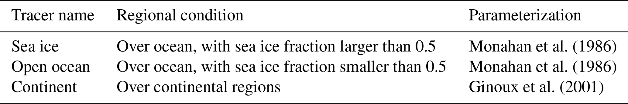
The parameterizations refer to the application of the condition to wind speed.

2.1.3 Tracer interpolation at Arctic sites

The concentrations of each tracer are interpolated daily at the coordinates of five Arctic stations: Alert (Canada), Ny-Ålesund (Svalbard), Tiksi (Russia), Utqiaġvik (Alaska), and Villum (Greenland). Series of the simulated concentrations of the three tracers can therefore be set up. The five stations were chosen for their distribution around the Arctic basin (Fig. 1e). This distribution sets the conditions for assessing the spatial sensitivity of the method in this region. Furthermore, many measurement campaigns are conducted at these stations (e.g., the Ny-Ålesund Aerosol Cloud Experiment, NASCENT (Pasquier et al., 2022)).

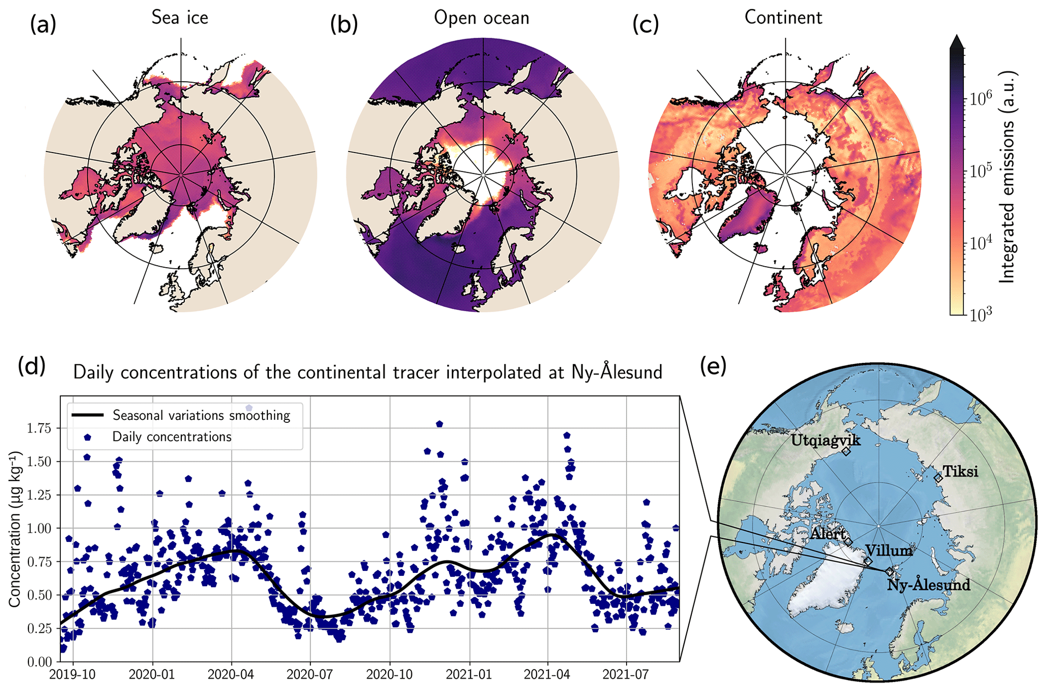
Figure 1 Overview of the tracer emissions in WRF-Chem and concentration series reconstructions. Regions of emissions of sea ice (a), open-ocean (b), and continental (c) tracers. (d) Example of reconstructed series of daily concentrations interpolated at Ny-Ålesund. (e) Map of the Arctic with the locations of the five studied stations. Base map from Cartopy © British Crown copyright 2016.

Figure 1 presents the emission regions (panels a, b, c) of the three tracers in terms of their integrated emissions over 1 year of simulation. Panel (d) shows an example of a reconstructed series of concentrations interpolated at the coordinates of the Svalbard station, Ny-Ålesund. A seasonal variability in the concentrations can be clearly detected, which is in accordance with actual observations of Arctic species. This variability is mainly due to seasonal variations in mesoscale atmospheric transport and in local wind speeds (both being phenomena reproduced by WRF). Nevertheless, not all simulated concentration series show such a variability; it depends on the tracer and the station. The strongest variability is found for the continental tracer; the lowest variability is found for the sea ice one. More broadly, the farther the emission source from the station, the weaker the observed variability.

Reproducing real concentration series is not in the scope of this study. Therefore, even though the tracers have aerosol-particle-like properties, the interpolation of their concentrations does not mimic what is seen with the instrumentation used for this type of measurement. Consequently, it is important to note that these series cannot be assimilated to actual concentrations of any atmospheric species.

The knowledge of the tracer emission conditions peculiar to this experiment allows for the evaluation of the method performances. Theoretically, a perfectly working method of tracking would point out the exact sources of emission that correspond to each tracer. Practically, the performances of backward methods are heterogeneous among tracers and from one station to another. Section 3.3 discusses the way the method should be applied in order to get the best performances and what parameters drive its success.

2.2 PES plumes with FLEXPART-WRF

FLEXPART belongs to the family of Lagrangian particle dispersion models (LPDMs). These are stochastic tools for the modeling of large amounts of air tracers. The Lagrangian approach allows for reduced numerical diffusion (Cassiani et al., 2016), which therefore leads to better capturing of atmospheric diffusion than with Eulerian models (Pisso et al., 2019). LPDMs also show the advantage of remaining independent of the model grid resolution since they use a Lagrangian approach. This accounts for the recommended utilization of LPDMs for the interpretation of PES in source tracing (Stohl et al., 2002).

FLEXPART (Pisso et al., 2019) simulates emission, diffusion, and deposition processes (wet and dry) or time-based decay of atmospheric tracers. The emission is done through single or multiple volume sources, and the simulation can be run forward or backward in time. The path of the emitted tracers is followed through a plume representation expressed in terms of PES in seconds. It can be likened to the residence times of particles in each grid cell. This information surpasses the direction of the origins commonly given by simple trajectories (Hirdman et al., 2009). The FLEXPART performances have been validated with multiple atmospheric-tracer-release experiments (Stohl et al., 1998). Furthermore, Hegarty et al. (2013) demonstrated FLEXPART's ability for reconstructing the dispersion of atmospheric tracers.

When investigating ground emissions, it is common to introduce the footprint PES (FPES), defined as the PES of the first FLEXPART vertical level. This will be defined here as the first 100 m above ground level. Here, we use the FLEXPART-WRF version of the model. It is optimized to use the WRF output data (see Sect. 2.1), allowing for the controlling of meteorological variables through WRF. In FLEXPART-WRF, several FLEXPART schemes are replaced by the WRF's ones (Brioude et al., 2013). This is intended to give information on the particle origins. The accuracy of the transport patterns simulated by FLEXPART-WRF decreases with the augmentation of the backward-simulation duration and relies on the accuracy of the initial WRF simulation in terms of meteorological variables.

2.2.1 Emission configuration in FLEXPART

The tracers in FLEXPART are characterized by five parameters (Table 2). First, we define the release time of the particles. In our case, the model emits over a whole day, corresponding to the associated in situ measurement (Sect. 2.1.2). Then, we set the release box, which is defined as a 50×50 km wide and 10 m high box. The trajectories are computed backward in time for 7 d before the time of release. A total of 100 000 particles are released in the emission box. The sensitivity of the PES plume to the number of released particles is inversely proportional to this number. Although this sensitivity is low, a rate of 10 000 particles emitted per hour is recommended. Finally, we can set different schemes for the tracers' dry and wet deposition. For the experiment depicted in Sect. 2.1.2, we set an exponential decay similar to that of the WRF-Chem tracers used to construct the concentration time series.

Table 2 Emission parameters for FLEXPART-WRF.

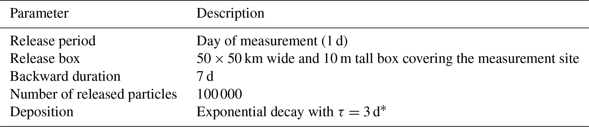
^* Deposition parameters can be set differently depending on the studied species.

The complete FLEXPART-WRF configuration file used here is available (cf. “Code and data availability” section). FLEXPART-WRF is run for every day of the synthetic concentration series (715 d at the five different locations) with the parameters described above. Finally, the ratio method (Sect. 2.3) is applied to the FLEXPART-WRF outputs, and the results are analyzed for the three tracers (sea ice, open ocean, continent) independently.

2.3 Statistical source identification method

In this study, we work on a statistical analysis method for back trajectories or PES that relies on the computation of PSCFs. The method itself is inspired by the analysis protocol introduced by Ashbaugh (1983) and Ashbaugh et al. (1985). Since then, backward models have evolved significantly, and the method has been used in many studies on the sources of atmospheric species (Sect. 1). In the following, we will stick to the PSCF methodology introduced in Hirdman et al. (2010) without the bootstrapping post-analysis, which is how it is mostly applied in the studies that use it. This will be referred to as the “ratio method”.

The approach relies on both atmospheric species concentration measurements and model outputs from FLEXPART-WRF. For each point of the concentration series, a FLEXPART-WRF simulation is run in backward mode. Then, the outputs of every run are sorted according to the measured particle concentration they are associated with. The great majority of earlier studies relying on backward analysis stop here without further analysis. However, this level of analysis only allows information on the direction of origin, with proximity bias near the measurement site. In the present study, we use a deeper analysis, which is described below.

Let us consider S_t to be the average of the FPES fields from a set of N FLEXPART-WRF runs:

$$\begin{array}{}\text{(1)}& S_{\text{t}}={\displaystyle \frac{\mathrm{1}}{N}}\sum _{n=\mathrm{1}}^{N}S\left(n\right),\end{array}$$

where N is the number of model runs, and S(n) is the array of FPES associated with the measurement n.

S_t can be interpreted as the climatology of the origins of air masses that are associated with the particle concentration series in the studied period. We can sort the concentrations in order to select the $P=\frac{x\times N}{\mathrm{100}}$ highest and lowest concentrations, with x being the percentage of selection. Thus, if S is the series of FPES fields sorted from the lowest to the highest measurement value, we can define $S_{\text{h}}^x$ and $S_{\text{l}}^x$ as the climatologies of the origins of air masses associated with, respectively, the P highest and lowest particle concentrations. These new fields are expressed as follows:

$$\begin{array}{}\text{(2)}& {\displaystyle }{S}_{\text{h}}^x& {\displaystyle }={\displaystyle \frac{\mathrm{1}}{P}}\sum _{n=N-P}^{N}S\left(n\right),\text{(3)}& {\displaystyle }{S}_{\text{l}}^x& {\displaystyle }={\displaystyle \frac{\mathrm{1}}{P}}\sum _{n=\mathrm{1}}^{P}S\left(n\right).\end{array}$$

As the PES decreases with distance from the measurement site, a proximity bias is observed in these climatologies, giving the impression of mainly local sources. To eliminate that bias, we compute the ratio of $S_{\text{h}}^x$ ($S_{\text{l}}^x$) to the total climatology S_t. We can thus define $R_{\text{h}}^x$ and $R_{\text{l}}^x$, the respective ratios of the high and low climatologies:

$$\begin{array}{}\text{(4)}& {\displaystyle }{R}_{\text{h}}^x& {\displaystyle }={\displaystyle \frac{P}{N}}{\displaystyle \frac{S_{\text{h}}^x}{S_{\text{t}}}},\text{(5)}& {\displaystyle }{R}_{\text{l}}^x& {\displaystyle }={\displaystyle \frac{P}{N}}{\displaystyle \frac{S_{\text{l}}^x}{S_{\text{t}}}}.\end{array}$$

Values equal to $f=x/\mathrm{100}$ indicate no deviation from the average field S_t. Consequently, the points where $R_{\text{h}}^x$ is higher than f correspond to the regions of likely origin for the studied particles. The same reasoning being applied to $R_{\text{l}}^x$ leads to the conclusion that the corresponding field no longer indicates the presence but rather indicates the absence of sources or even the presence of sinks.

One should be aware that the significance of $R_{\text{h}}^x$ and $R_{\text{l}}^x$ is proportional to the value of S_t. Low values of S_t indicate little transport through the corresponding grid points and therefore can invalidate the statistical results of the ratio computation. Practically, too-high values of the ratio can be suspected to be spurious indications. However, if the percentage x is strict (i.e., low) enough or if the total number N of runs is large enough, these excessively high values should not appear.

In the following, we will discuss further how to define a threshold of FPES in order to prevent false interpretation of the ratio fields. Because the ratio method allows us to eliminate the FLEXPART proximity bias, it can miss the detection of very local sources when applied to a large domain. However, due to this effect being proportional only to the domain size and resolution, it can be mitigated by either increasing the resolution or downscaling the domain.

3 Results

3.1 Metric of evaluation

The main result of the ratio method is the ratio map associated with the highest concentrations of the studied series. By itself, it gives qualitative information on the source origin of the species. In order to get some quantification, we use the definition of the surface types that corresponds to the tracer emissions (Table 1). Masking the ratio maps with continental, open-ocean, and sea ice masks and then summing the ratio values corresponding to these surface types, we get a quantification of the actual detection performed by the method. We introduce the detection score D_T, defined as follows:

$$\begin{array}{}\text{(6)}& D_T={\displaystyle \frac{R_T}{R}},\end{array}$$

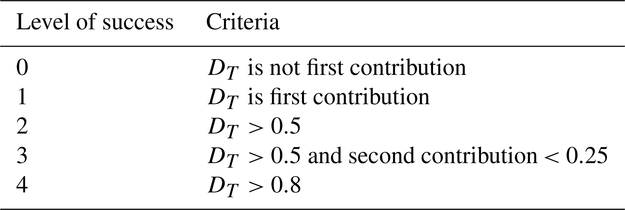
where D_T refers to the signal contribution of the surface type corresponding to the tracer T (sea ice, open ocean, continent), R is the result signal ($R_{\text{h}}^{\mathrm{10}}$ in the standard method or R_10–33 in the improved method; cf. Sect. 3.3), and R_T is the sum of R over the surface type corresponding to the tracer T. A perfect detection would be a full contribution of the surface type that corresponds to the analyzed tracer, i.e., D_T=1. For instance, the method applied to the concentrations of the continental tracer should lead to the detection of the continent, with a limited contribution of sea ice and open-ocean regions. In that case, D_T would tend toward 1. Practically, the ratio method gives various results. Therefore, a metric with five levels of success has been defined to catch the fluctuations in the method performances. Table 3 describes the metric levels. Good confidence is attributed to the results when level 2 is reached. Levels 0 and 1 call for special attention and map analysis.

Table 3 Definition of the criteria for the evaluation of the ratio method results.

3.2 The standard ratio method

In this section, we use the ratio method, or the PSCF method, as presented in Sect. 2.3. We apply it to the simulated data constructed with the numerical experiment presented in Sect. 2.1.2. For clarity, we present one case: retrieving the sources of continental-tracer emissions from the Ny-Ålesund simulated concentration series.

Figure 2 illustrates the application of the ratio method to one of the tracers simulated in the idealized experiment (Sect. 2.1.2). The ratio maps for the three tracers and the five stations are available in the Supplement (Fig. S1). Panel (a) shows the concentration series of the continental tracer interpolated at Ny-Ålesund over 2 years of simulation. The highest and lowest concentrations are flagged with, respectively, red and cyan colors. The second line in Fig. 2 is dedicated to the maps of FPES (panels b and c) and to the ratio map (panel d). The map in (b) corresponds to the S_t defined in Sect. 2.3. It is the climatology of the origins of all of the air masses ending at Ny-Ålesund over the 2 years of simulation. Similarly, (c) shows $S_{\text{h}}^{\mathrm{10}}$, the climatology of the air mass origins that contained the 10 % highest continental-tracer concentrations of the series. Finally, (d) shows the ratio of $S_{\text{h}}^{\mathrm{10}}$ over S_t, which has been presented as $R_{\text{h}}^{\mathrm{10}}$. This ratio map or PSCF map is the map resulting from the ratio method. It shows various regions of likely sources for the continental-tracer time series. While Greenland and Canada are the main sources identified, there are also less continuous signal spots in Eurasia. Even though there is some signal overflow over the North Pacific and Baffin Bay and a small amount over the Arctic Ocean, the quantification metric (defined in Sect. 3.1) gives, in this case, a score of 2. This means that the continental source is correctly detected.

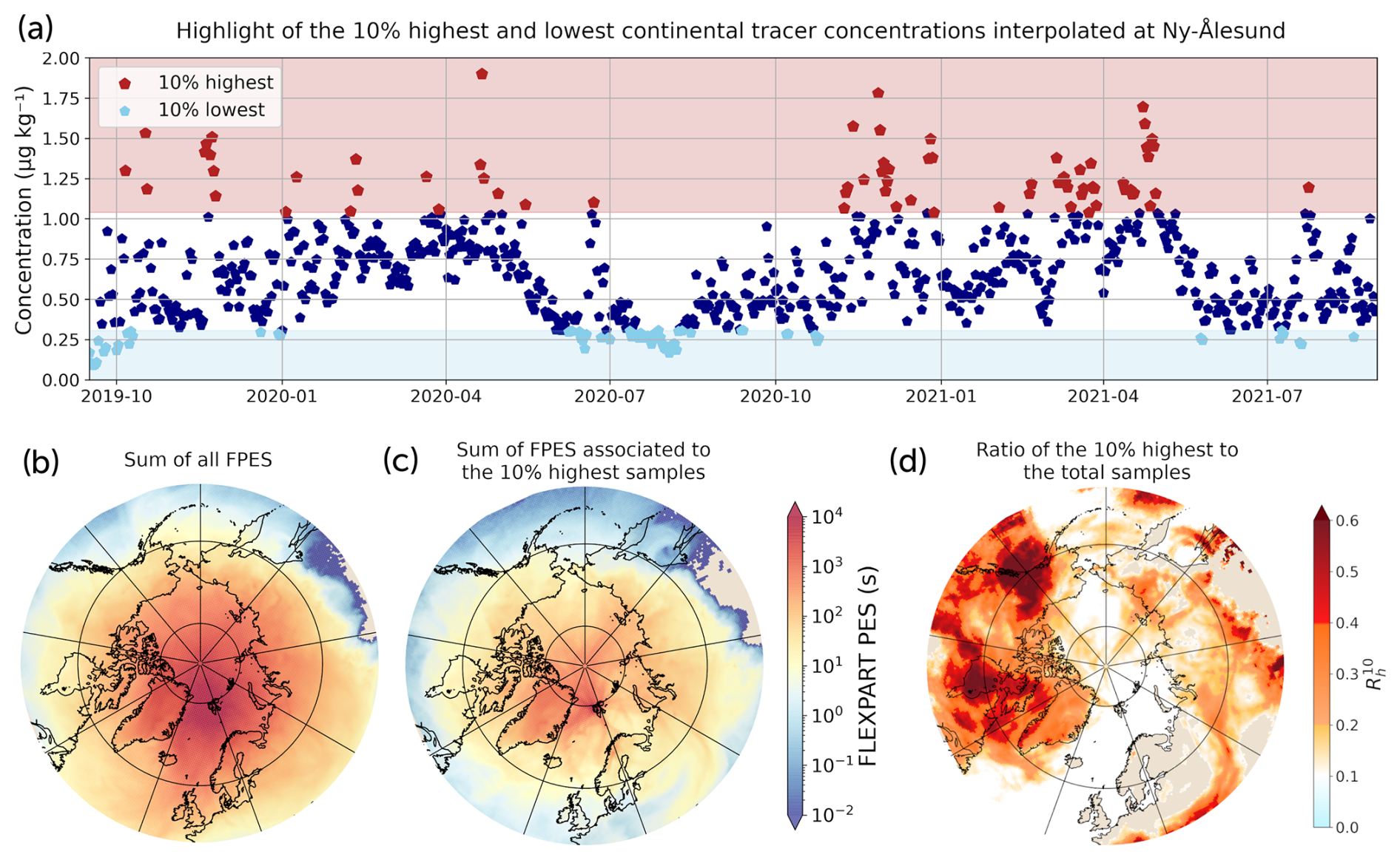
Figure 2 Application of the ratio method as it is depicted in Sect. 2.3. Panel (a) shows the reconstructed daily concentration series of the continental tracer interpolated at Ny-Ålesund over the 2 years of simulation. Panel (b) shows the climatology of the total air mass origins; panel (c) shows the climatology of the origins of air masses that brought the 10 % highest concentrations; and panel (d) shows the ratio of (c) to (b), noted as $R_{\text{h}}^{\mathrm{10}}$.

The results for the continental tracer of the other stations (Alert, Tiksi, and Utqiaġvik but not Villum) are shown to be successful (as will be seen in Fig. 4a). Nevertheless, the application of the method to both sea ice and open-ocean tracers gives poor results. Only Ny-Ålesund and Tiksi show a correct detection for the open-ocean case. Otherwise, all the other detections fail, showing the continent to be the main contributor (Fig. 4a). This observation brings into question the reliability of the continental-tracer results. Indeed, a geographical bias strengthens the continental signal. We can identify three reasons for this behavior. Firstly, the domain of the simulation tends to over-represent continental regions. Indeed, the continent accounts for 53 % of the total surface area, while the open-ocean and the sea ice regions represent, on average, 37 % and 10 %, respectively. In the idealized situation of exact back-tracking of the air masses, this bias should not affect the detection results. However, dispersion modeling is innately imperfect. The computation of the ratio induces a loss of information on FPES intensity. The latter is replaced by the ratio values which can reach a saturation value of 1 for regions where very few FPES plumes pass. If an area is covered only by FPES plumes associated with the highest concentrations of the measurement series, we get a saturation of the ratio. Thereby, regions of very low FPES can end up being highlighted on the ratio map even though they do not show statistically significant values. Consequently, irrelevant signals affect the detection, likely benefiting the predominant surface type, namely the continent in this Arctic situation. Secondly, and to a lesser extent, the other reason for biased results is the seasonal variability of the concentration series. As described in Sect. 2.1.2, the simulated concentrations vary during the year, with maximum concentrations in winter and spring and low concentrations in summer and autumn, following the well-known Arctic haze seasonal cycle. The latter is due to efficient transport of air masses from land masses in the mid-latitudes during spring (Schmale et al., 2022). As a result, applying the ratio method to annual observations of short-lived pollutants in the Arctic produces a climatology of air mass origins in winter and spring and is biased for lower-latitude sources, over-representing continental sources, as seen in our evaluation in Fig. 4a. Last but not least, any source attribution method based on a single observation site will suffer from a so-called “shadowing” effect. This tends to falsely assign emissions to areas that are upwind of the true emitting area. In the present case and for the sea ice and ocean tracers, the continental areas are mostly in such a configuration. The only way to robustly overcome this problem is by using a network of sites that can observe gradients across the domain or at least observe the same source area under different flow directions (as demonstrated in Sect. 3.5). These implications suggest that the ratio method, as applied in this section, is not suitable for studies involving real measurement data.

The next section will present and discuss the improvements that make the method reliable for real case studies.

3.3 Improving the ratio method

In Sect. 3.2, the standard ratio method gave ambiguous results. In this section, we present how one can improve the method in order to get more reliable source identification.

To eliminate the seasonal variability bias, we sort the concentrations based on their differences in relation to the seasonal trend of the series rather than sorting them according to their absolute values. Practically, we estimate the seasonal trend by fitting the series and then subtracting it from the concentrations. This is similar to the background subtraction methods of Ruckstuhl et al. (2012) and Resovsky et al. (2021). Practically, we estimated the background seasonal concentration by smoothing the series with a locally weighted scatterplot smoothing (LOWESS) filter and then subtracting the background trend from the concentrations to keep the high-frequency signal from recently added emission events.

Concerning the over-representation of the continental area, a cutting threshold of FPES is set in order to filter the less significant FPES. This is similar to the approach of Fang et al. (2018), who suggested excluding grid cells crossed by too few trajectories. The values of S_t, S_h, and S_l under this threshold are removed for the ratio computation. The risk with this tuning is the loss of information while filtering the lowest FPES values. We performed tests in order to identify the best threshold using the idealized-tracer experiment for the assessment. The details of this experiment are discussed in Sect. 4. The best results are obtained for a variable threshold that filters out the 2 % lowest FPES of the studied case. The threshold varies from one case to another in order to always remove the 2 % lowest FPES values. It is worth noting that applying a filter to FPES or PES values is, on average, equivalent to setting a threshold for the number of trajectories passing through a grid cell. In this manner, we remove the majority of FPES values which are less statistically significant.

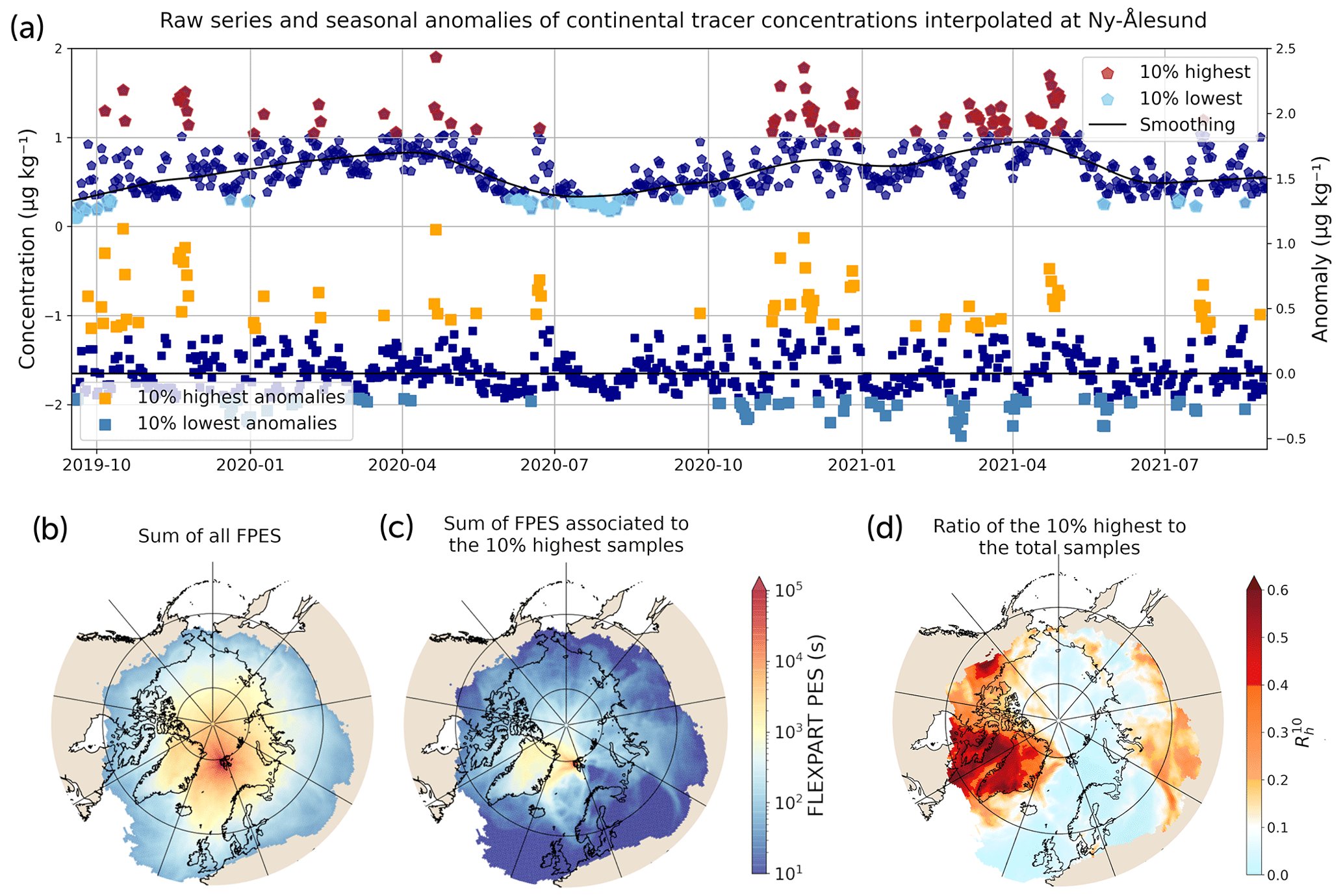
Figure 3 Application of the improved ratio method. Similarly to Fig. 2, (a) shows the reconstructed daily concentration series of the continental tracer interpolated at Ny-Ålesund with the comparison of the standard sorting (top) and the seasonal sorting (bottom). Panel (b) is the climatology of the total air mass origins; (c) is the climatology of the origins of air masses that brought the 10 % highest concentrations; and (d) is the ratio of (c) to (b), noted as $R_{\text{h}}^{\mathrm{10}}$. In (b) and (c), the 2 % lowest FPES values have been removed, as explained in Sect. 3.3.

These two modifications to the ratio method are illustrated in Fig. 3. Panel (a) displays the original concentration series with the classical sorting of high and low values (top), as well as the series constructed with the differences in terms of the seasonal variations (bottom). The highest values of the latter are flagged in yellow. They are more evenly distributed over the simulation period than the raw concentrations. The effect is even clearer for the lowest concentrations; some of the lowest points happen in the cold season, which was never the case with the standard sorting method. Panels (b), (c), and (d) highlight the effect of the filtering threshold on FPES. Indeed, removing the 2 % lowest FPES values erased a corona of values clearly visible on the climatology maps. The ratio map of panel (d) presents a much smaller area of values above 0.1. The overflows over sea ice and open-ocean regions are greatly reduced. Baffin Bay is the region where an incorrect signal remains. This shows that shadowing can still happen, especially around regions of intense emissions. The North American and Eurasian signals decreased as well. Even though they correctly corresponded to continental emissions, their significance is considered to be low because they were due to regions of low FPES. The quantification of the detection indicates a level of success of 3 for this case, while the standard method only gave a value of 2.

In order to take maximum advantage of the ratio method, the information contained in the ratio associated with the lowest concentrations can also be used. Indeed, this ratio points to the regions where the sources are not likely to come from. Thus, its reverse (1−R_l) can be used as a mask applied to R_h. We use $R_{\text{h}}=R_{\text{h}}^{\mathrm{10}}$ and $R_{\text{l}}=R_{\text{l}}^{\mathrm{33}}$. Thus, we get a composite ratio, which is defined as follows:

$$\begin{array}{}\text{(7)}& R_{\text{10–33}}=R_{\text{h}}^{\mathrm{10}}\times (\mathrm{1}-R_{\text{l}}^{\uparrow \mathrm{33}}),\end{array}$$

where $R_{\text{l}}^{\uparrow \mathrm{33}}$ denotes the values of $R_{\text{l}}^{\mathrm{33}}$ above 0.33. We choose to use $R_{\text{l}}^{\mathrm{33}}$ rather than $R_{\text{l}}^{\mathrm{10}}$ and $R_{\text{l}}^{\mathrm{5}}$ because it considers more PES, and, thus, it is a more statistically significant ratio. Additionally, unlike the ratio of high concentrations, we aim to select as many regions as possible that are detected as unlikely sources. To our knowledge, taking into account these areas of low concentrations in a PSCF method has not been tried in the past and is the most innovative part of our method. Testing the detection performances of the composite ratio showed improvement in 6 out of 15 cases and enhanced the number of correct attributions in 80 % of the cases. We therefore include the composite ratio as a final step for the improved ratio method.

The details of the performance improvements for each modification presented above are given in Table 4 and discussed in the next section (Sect. 3.4).

3.4 Result comparison

The success levels allow for an easy comparison between the different ways the method is applied. Therefore, we can compare the performances of the standard method – as if we were to apply the ratio method described in Sect. 2.3 straightforwardly – with the results of the improved method presented above. Figure 4 illustrates these results.

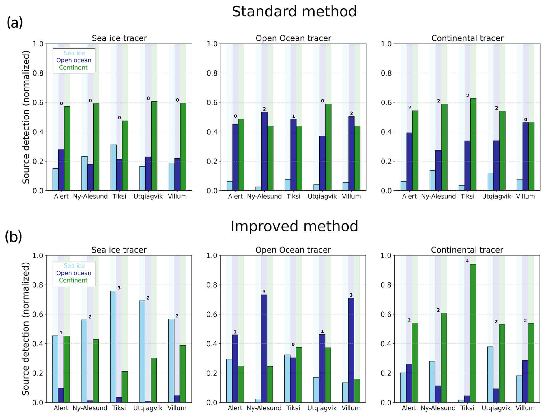
Figure 4 Comparison of the results obtained with the standard ratio method (a) and with the improved ratio method (b). Every panel presents the detection results for a specific tracer and for the five stations. The bars represent the contributions of each surface type to the detection (light blue for sea ice, blue for open ocean, green for continent). For every pair of tracer and station, the level of success is shown above the corresponding bars.

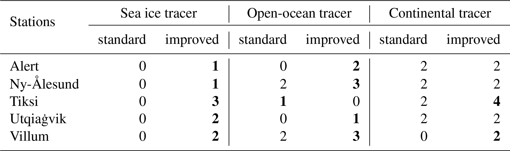
As mentioned in Sect. 3.2, the assessment of the standard method (Fig. 4a) does not provide a level of confidence high enough for us to trust its results. The improved method performs better in 10 out of 15 tested cases (Fig. 4b), worse in 1 case, and equally otherwise, as reported in Table A2. As expected, the overall contribution of the continental source decreased thanks to the FPES filtering threshold. The open-ocean source suffered the same effect. The improved method detects much more accurately the origins of the open-ocean, continental, and sea ice tracers, with correct attributions at four out of five stations for the ocean tracer (three in the original method), at three out of five stations for the ice tracer (zero in the original method), and at five out of five stations for the continental tracer (four in the original). In addition, the quality of the detection score is improved or identical and is degraded in only one case (open-ocean tracer at Tiksi). The detection level averaged over the five stations and three tracers gives a general assessment of the methods. The standard ratio yields an averaged score of 0.9, which corresponds to a failed detection, as defined in Sect. 3.1. The improved ratio method yields a score of 2.0, which is where the threshold for good confidence in the results starts.

However, a few detections still fail. Figure S2 in the Supplement shows the composite ratio maps of the improved ratio method for all the stations and the three tracers. It enables the detailed examination of the identification results. The source detection of the sea ice tracer at Alert is highly polluted by the continental signal. The composite ratio maps of this case give insight into the reason for this fail, presenting an overflowing shadowing of the plume in the continental regions (cf. Sect. 3.2). The poor detections of the open-ocean tracer at Alert and Utqiaġvik are due to hard shortening of the FPES from the threshold filtering. The plume mainly covers the regions of marginal sea ice. We observe the same thing for Tiksi, even though the map clearly shows the influence of both the North Pacific and the North Atlantic. Regardless, for all cases, the composite ratio maps give great information on the region of origin.

In order to assess the contributions of the three modifications (FPES filter, background subtraction, composite ratio) to the standard ratio as introduced with the improved ratio, the source identification has been run in the standard ratio setup with one or two modifications from the improved ratio. The results are presented in Table 4. Each cell value corresponds to the averaged success level when the column and row modifications are used. Thus, the diagonal values refer to the detection score when a single modification is used in addition to the standard ratio, and the others refer to the detection score when both the row and column modifications are used. The highest improvement is due to the FPES filtering, with an improvement of 0.4 compared to the standard ratio. The composite ratio allows for a 0.2 rise, where the background subtraction leads to an improvement of only 0.1. The best combination appears to be the composite ratio with the FPES filter, which improves the score of the standard method by 0.7. The combination of the composite ratio and the background subtraction only accounts for a 0.2 improvement. Even though the latter seems to be a small improvement, the full potential of the improved ratio method is only reached when the three modifications are used all together. In other words, the three modifications are needed to reach an averaged detection level of 2, which is the threshold of a confident successful detection (Sect. 3.1). The detailed performances of these tests (i.e., for the three tracers and five stations) are presented in the Supplement (Fig. S3).

Table 4 Comparison of the averaged success levels when adding the different modifications to the standard ratio. Each cell gives the averaged level of detection when the column and row modifications are added to the standard ratio methodology. The corresponding score of the standard ratio is 0.9, and the score is 2.0 for the improved ratio.

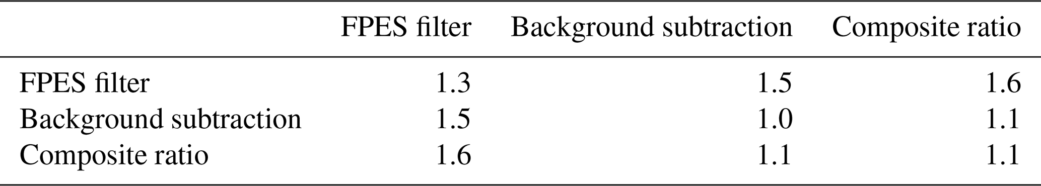
The values are rounded to the first two digits.

3.5 Combination of stations

Some observations of atmospheric species are made within a measurement network composed of multiple experimental sites (e.g., ICOS, WMO GAW, NOAA flask network, AGAGE). The observations can therefore be simultaneous and equally distributed in time. This tends to draw a snapshot of the state of the atmosphere with regard to the studied species or variables. This can also be achieved with satellite data, from which it is possible to interpolate quasi-simultaneous time series at many different locations around the globe.

We can envision that the species of interest in this study are or will be part of an observational network or measured by satellite observation. Therefore, how would the tracing method presented here take advantage of this? In order to answer that question, we compute the method combining the FPES associated with the five Arctic stations previously described as a way of triangulating the sources. Once again, we are in the presence of an idealized situation: the concentration series are perfectly simultaneous and derived identically. True observational data might drift from these perfect conditions; however, we believe that this experiment can illustrate the potential of such an application of the method.

For the combination, we kept the sorting of high and low concentrations specific to each station. We also did this for the sorting of the corresponding FPES plumes. The gathering is done at the step of ratio construction. S_h and S_l are computed as the sum of the corresponding ratios of every station. In the same way, the total climatology of the FPES plumes S_t is now the sum of the PES plumes of the five stations. The ratios R_h and R_l are then calculated with Eqs. (4) and (5).

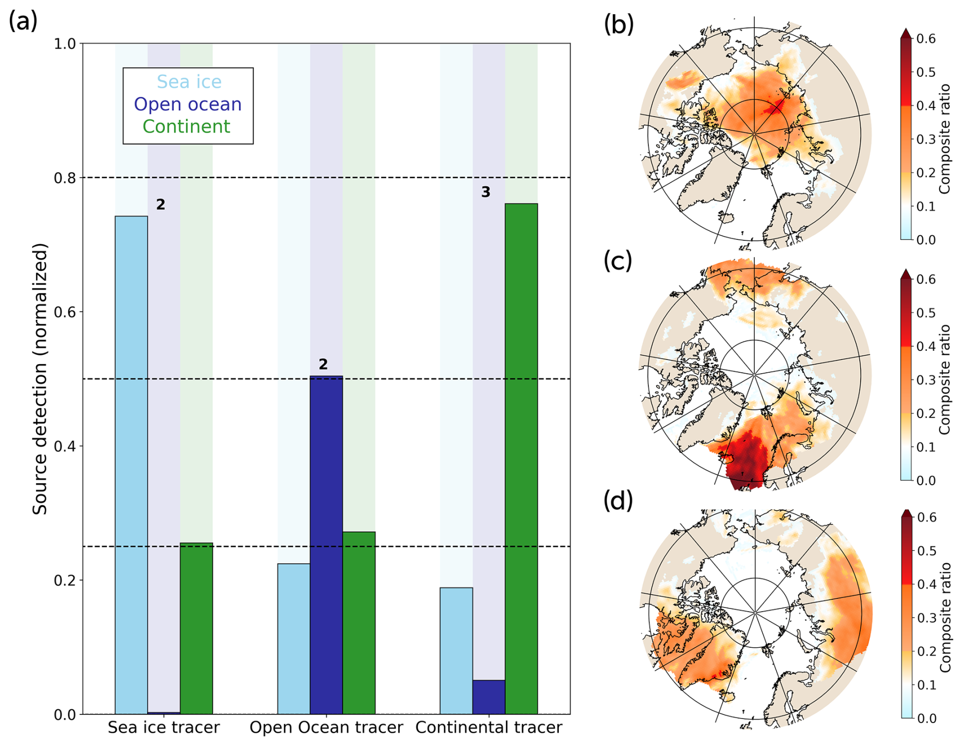
Figure 5 Results of the combination of the five stations. Panel (a) shows the fraction of the contribution of every surface type for the three tracers and the associated success level. Panels (b), (c), and (d) are the composite ratio maps for the sea ice tracer, the open-ocean tracer, and the continental tracer, respectively.

The results show a successful source origin detection (Fig. 5). The continental sources are detected with a success level of 3, while the sea ice and open ocean yield a success level of 2. This lower score for the open ocean could be explained by the geographical arrangement of the stations: open-ocean regions are not well surrounded by the Arctic stations. While Villum and Ny-Ålesund are exposed to North Atlantic sea sprays, Utqiaġvik is hardly reached by these emissions. Conversely, the North Atlantic stations do not get much signal from North Pacific emissions. More generally, sea ice and open-ocean results are affected by some continental signal due to systematic coastal overflow. This effect leads to lower scores even though the composite ratio maps give clear insights into the origin regions. The existence of this unshrinkable surfeit of continental signal should be kept in mind when interpreting any results of similar applications of the method.

Nevertheless, the combination of simultaneous observations of the same species has the potential to give precise clues regarding the regions of origin of the so-called species. The implementation of data from mid-latitude stations could also improve the results by increasing the spatial coverage. Therefore, the present work encourages the development of observational networks or coordinated field experiments dedicated to identifying short-lived species at the high latitudes, following the example of the networks for greenhouse gas observations that are used to attribute global and regional emissions. The global deployment of the Portable Ice Nucleation Experiment (PINE) (Möhler et al., 2021) fits this recommendation for the study of INPs.

3.6 Points for using a ratio methodology

We note that we did not test the improved ratio method against raw FPES interpretation. In order to get an idea of how they compare, Fig. 6 shows, through the example of the sea ice tracer for the Tiksi station, different visualizations of the FLEXPART-WRF FPES. The first line shows the climatologies of the FPES over the period of observation. These representations are often used for quick qualitative source identification in studies using back trajectories or PES (Fig. 6a and b). The second line shows the results of the ratio methods presented in this paper. What the figure reveals is that the sea ice origin of the tracer is only clearly found with the improved ratio method (Fig. 6d and e). As a reminder, if the source detection was perfect, the light-blue bar would reach 1 in Fig. 6e since the studied tracer was only emitted in sea ice regions. The climatologies, particularly those in Fig. 6b, provide general information about potential sources of the tracer. However, this does not allow for reliable quantification, as seen in the corresponding column in Fig. 6e. Likewise, the standard ratio method does not allow this either (Fig. 6c), giving – in this case – even worse quantification results than the climatology. Let us mention that weighting the FPES plumes with the particle concentrations has also been tested, and this did perform similarly to the climatology of the highest observed concentrations. Ultimately, only the improved ratio method provides a clear map of the actual origins of the tracer (Fig. 6d compared to Fig. 1a) and enables unequivocal quantification of it.

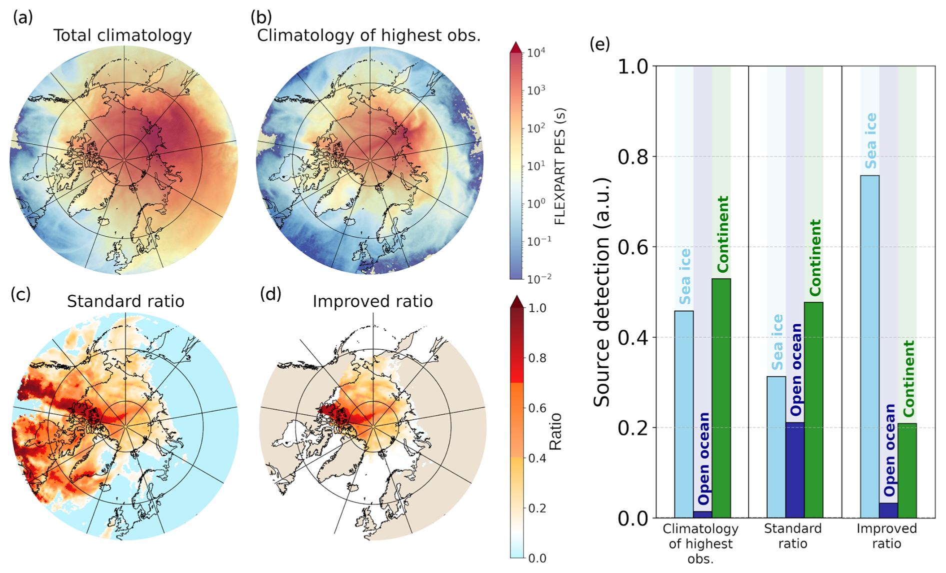
Figure 6 Panel of FPES visualizations and analysis for the sea ice tracer at the Tiksi station. Panels (a) and (b) are the climatologies of, respectively, the total FPES value and the values associated with the 10 % highest observations ($S_{\text{h}}^{\mathrm{10}}$). Panels (c) and (d) are the ratio maps of the two versions of the ratio method ($R_{\text{h}}^{\mathrm{10}}$ for, respectively, the standard and improved versions). Panel (e) is the quantification of the detection results for the climatology associated with the highest observation and for both versions of the ratio method.

4 Discussion on sensitivities

In this section, we investigate the sensitivity of our improved ratio method to key parameters: the sorting percentiles, the data series duration and frequency, and the filtering threshold of FPES.

4.1 Sorting percentiles

The standard ratio method uses the 10th percentile to sort the highest and lowest points of the measurement series. A higher threshold would address more points, which could be needed for statistical representativeness when the series is short. Some studies use the 33rd or 36th percentile to define the highest measurements (Irish et al., 2019; Si et al., 2019). In such short series, selecting the highest third of measurements amounts to us looking at a few particular PES plumes, and the benefits of computing the ratio appear to be poor. For longer time series, using the 33rd percentile to define the highest measurements among the observations is too broad and makes the ratio unable to identify the sources of emissions. With such a high percentile, the method also detects some of the high-concentration events due to particular atmospheric patterns, as well as some events of lower concentration. This dims the source identification and makes it inefficient. Actually, the tests performed on the idealized tracers (Sect. 2.1.2) using the 33rd percentile for selecting the highest concentrations show that the method is never able to retrieve the emission sources of the tracers. Conversely, the 5th percentile does not allow for the selection of enough data points, leading to a misdetection of some of the main source regions. Finally, the 10th percentile, used by the standard ratio method, gives the best performance when used with 1- or 2-year-long series of daily measurements.

4.2 Series duration

The original experiment had a duration of 24 months, which corresponds to a complete double seasonal cycle. The sensitivity of the method to the duration and frequency of the concentration series is tested by reducing the number of points in the series. First, in order to test the sensitivity of the method to the time series duration, the experiment is reproduced for two periods of 12 months: in the first year and then in the second one. Then, in order to test the sensitivity of the method to the concentration sampling frequency, the concentration series is cropped to keep only one concentration point every 2 d. In other words, the number of points is divided by 2, keeping the same time extent as the original experiment (half frequency). Finally, only one point is kept every week (frequency divided by 7).

The results show that 2 years of analysis does not improve the precision of the method compared to the 1-year experiment. However, a difference is observed when measurements are only performed every 2 d: the success level loses one point on average. Furthermore, lowering the frequency of measurements down to one every week causes us to lose one additional level of success. In conclusion, increasing the time resolution enhances the method's performance. The sampling frequency should always be considered when applying the improved ratio method.

4.3 FPES filtering

The improved ratio method (Sect. 3.3) incorporates a filter to exclude the grid cells with the lowest FPES values – i.e., those penetrated by the fewest trajectories. This serves to remove the least statistically significant results, as well as particle dispersion modeling imprecision near the domain boundaries. In practice, FPES values are filtered by a threshold determined based on a percentage of the total FPES in the domain for a given case. The threshold should be kept as low as possible in order to avoid information loss. Nevertheless, when it is too low, some arbitrary results may remain. In order to evaluate the effect of this FPES threshold on the performance of the source detection method, seven thresholds are tested, from no filter to filtering 6 % of the lowest FPES values. Increasing the level of filtering shrinks the studied region around the starting point of the backward dispersion, i.e., the measurement station. Because of this and because the selected stations are located around the Arctic basin, as the filtering level increases, the representation of the sea ice regions gets stronger. In terms of the success level of detection, this improves the scores for the sea ice tracer but tends to lower them for the open ocean (Fig. 7a). Because the tests are performed on simulated tracers (Sect. 2), it is possible to use these findings to calibrate what threshold may give the most reliable and meaningful results for all tracers. In Sect. 3.1, the detection is rated to be successful when the D_T score is superior or equal to 2. In Fig. 7b, 1 is used for every detection that satisfies the above condition (i.e., D_T≥2). Therefore, a given tracer can have a maximum overall score of 5 (i.e., a successful detection for the five stations). The evolution of the scores in Fig. 7b shows that a filtering of 2 % is the optimal compromise. This is the lowest threshold for which the total score plateaus. Although the scores for sea ice and continent tracers reverse with a 3 % filter, this does not affect the total score, making it preferable to maintain the lowest possible filtering threshold. Consequently, for the Arctic domain studied in this paper, we recommend using a 2 % filtering threshold.

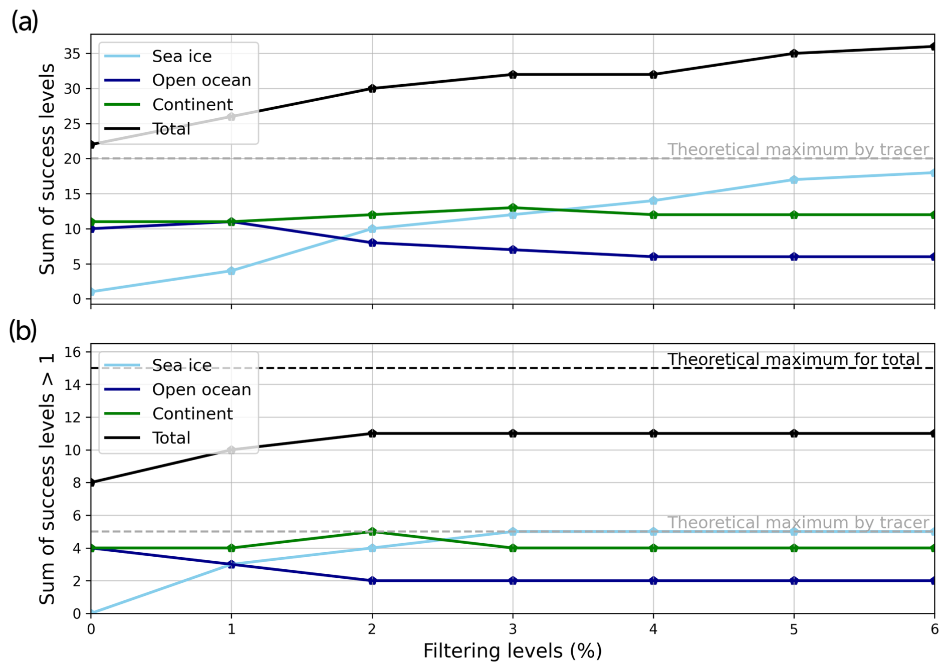
Figure 7 Evolution of the success level sum for different levels of low FPES filtering. In (a), the sum is performed based on the scores of the five studied stations (Alert, Ny-Ålesund, Tiksi, Utqiaġvik, Villum) independently for the three tracers (sea ice, open ocean, continent). The total success level is shown as a black line. Panel (b) takes only the success levels superior or equal to 2 and sets them to 1. Dashed lines represent the theoretical maxima of the individual tracer scores (gray) and of the total score (black).

5 Application examples on aerosol observational datasets

The improved ratio method presented in Sect. 3.3 has shown its capabilities in identifying the type (sea ice, open ocean, continent) of the emission sources of simulated atmospheric tracers. In this section, the method is applied to two observational datasets in order to test it under real conditions. The origin of the species observed in both datasets is well-defined: the first is continental, and the second is oceanic. This knowledge allows for a critical evaluation of the method's results. Discussing the results will provide clarity on how to apply the method correctly and how to accurately interpret its findings.

5.1 Aerosol absorption coefficient

The first dataset is a series of aerosol absorption coefficients measured at Zeppelin Observatory (Ny-Ålesund, Svalbard) at an altitude of 475 m above sea level between January 2019 and September 2022 (Eleftheriadis, 2019). For the application, we chose a 2-year period (September 2019 to August 2021), identical to the period during which the evaluation experiment was held (Sect. 2.1.2). The aerosol absorption coefficient measured at 550 nm is known to be mostly driven by black carbon (BC) concentrations as it is by far the strongest absorbing aerosol species in the visible spectrum (Bond et al., 2013; Kirchstetter et al., 2004). Consequently, we consider the aerosol absorption coefficient to be a marker of BC. BC is a great candidate for a first application of the method because its sources are relatively well known. A total of 90 % of the BC emissions are produced by continental sources, mainly biomass burning and incomplete combustion of fossil fuels from traffic and industrial activities (Bond et al., 2013).

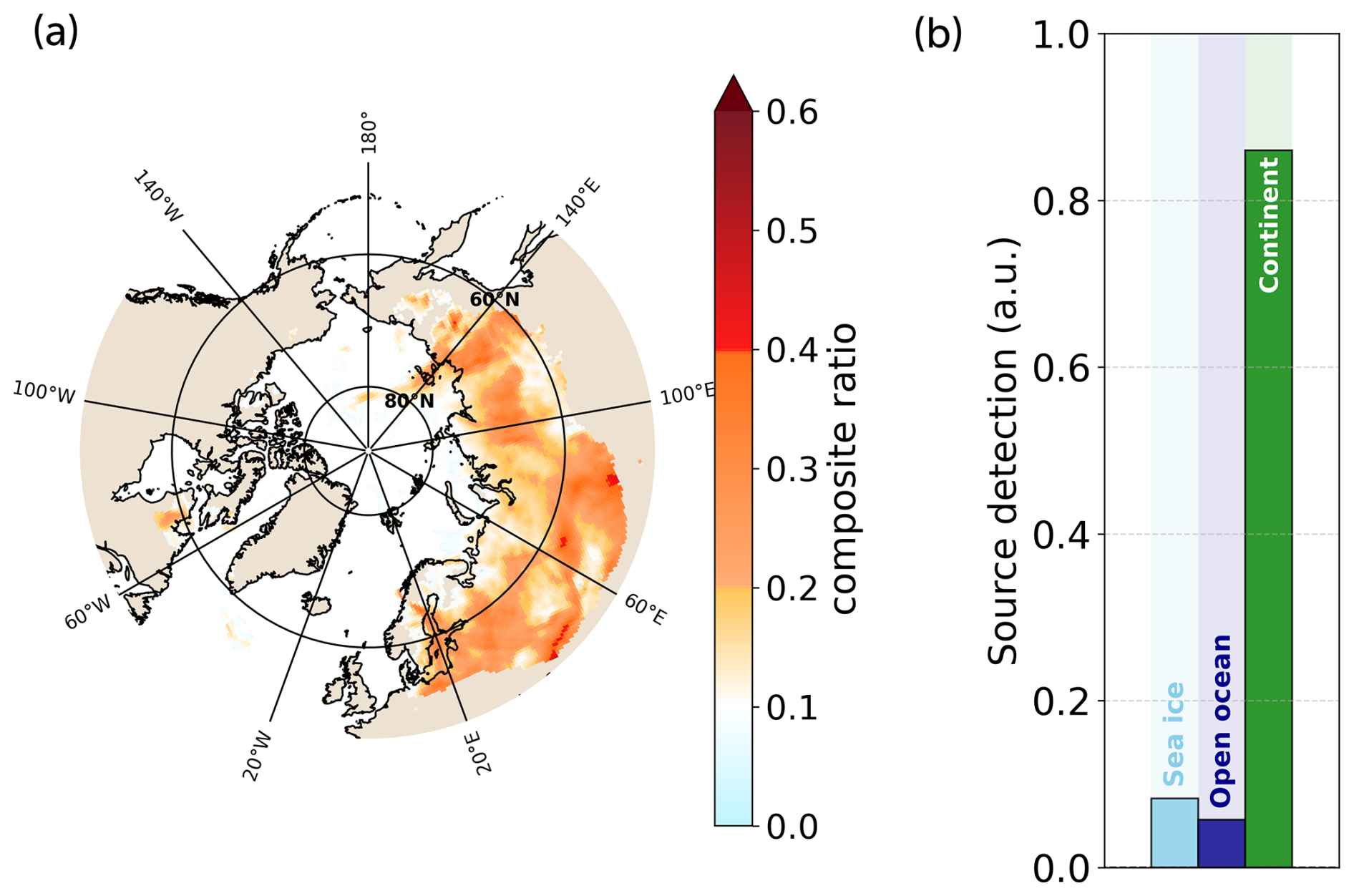
Figure 8 Results of the improved ratio method when applied to a data series of absorption coefficients measured at the Zeppelin Observatory (Ny-Ålesund, Svalbard). Panel (a) is the ratio of the improved method that highlights the likely regions of origin. Panel (b) is the quantification of the surface type contributions to the three sources (sea ice, open ocean, continent).

Figure 8 shows the ratio of the improved method as presented in Sect. 3.3 alongside the contributions of sea ice, open-ocean, and continental regions to the detection signal. Panel (a) highlights a strong Eurasian signal spreading from northern Europe all the way to eastern Siberia. Panel (b) confirms the continental origin, showing that more than 80 % of the signal comes from continental regions. Figure 4b showed that the detection of a continental-originating species at Ny-Ålesund could give spurious signals in oceanic regions (sea ice and open ocean). Therefore, the weak oceanic signals shown in panel (b) can be considered to be detection noise. The application of the improved ratio method to this series of BC measurements at Zeppelin Observatory unequivocally leads to the conclusion of a continental origin of the observed BC in Svalbard. This finding corroborates the results described in Winiger et al. (2016), Hirdman et al. (2010), and Xu et al. (2017), i.e., that BC observed at high-altitude sites comes from remote locations, mainly associated with Eurasian emissions.

5.2 Methanesulfonic acid

Methanesulfonic acid (MSA) is an organosulfuric compound. Its presence in the atmosphere is due to the emissions of dimethylsulfide (DMS). DMS is produced by marine bacteria and phytoplankton activity and can be oxidized into MSA in the atmosphere (Saltzman et al., 1983; Hopkins et al., 2023). Therefore, MSA measurements are expected to be associated with air masses of marine origins. Here, the dataset is a series of MSA particle phase measurements performed in the context of the Ny-Ålesund Aerosol Cloud Experiment (NASCENT) campaign held in Svalbard between September 2019 and August 2020 (Pasquier et al., 2022). The measurement series used in this study extends from January to December 2020. However, data are missing between July and August due to an instrument failure (Siegel et al., 2023). Similarly to the BC measurements (Sect. 5.1), the MSA measurements have been done at Zeppelin Observatory.

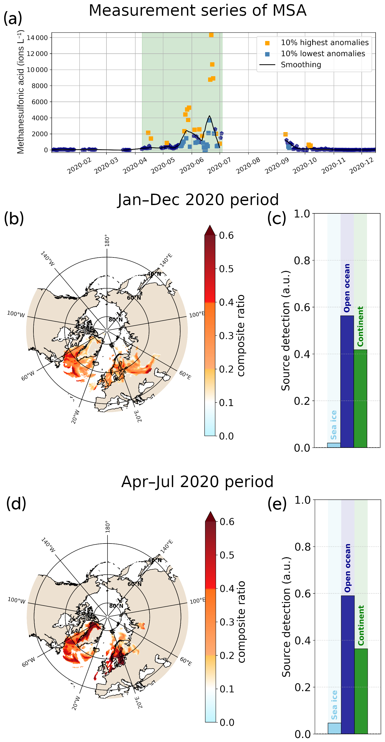
Figure 9 Results of the improved ratio method when applied to the data series of methanesulfonic acid (MSA) measured at Zeppelin Observatory. Panel (a) is the measurement series of MSA over 2020. The points corresponding to the 10 % strongest anomalies are represented in orange (high anomaly) and light-blue (low anomaly) squares. Panels (b) and (c) show the results for the complete series of measurements (January to December 2020). Panels (d) and (e) show the results for a period of continuous measurements of the dataset (April to early July).

The analysis of the results shown in Fig. 9 is non-trivial and should be taken as a textbook case of source identification by the ratio method. Panels (b) and (c) show the results for the analysis of the complete dataset extending over the whole year of 2020, while panels (d) and (e) show the results for the measurements between April and early July 2020. Panel (c) shows that, for the whole period of measurements, the main contribution is oceanic, but this is followed closely by the continental signal, while the sea ice region contribution amounts to almost zero. The ratio map shown in panel (b) indicates that two main spots stand out. The western one shows a strong signal in Baffin Bay, the Labrador Sea, and the Greenland Sea. Despite some overflow in continental areas, this spot mainly contributes to the oceanic signal and should be interpreted as such. The second spot spreads over northern and eastern Europe. The signal comes from the regions of the North Sea and the Baltic Sea, which are both regions of high chlorophyll-a (Chl-a) concentrations. Nevertheless, the main signal of this spot is over continental areas. A part of this may be ascribed to overflows, but the eastern strip has to be considered to be an actual signal. It points toward the north of the Caspian Sea, where the phytoplankton might be important (Eker, 2005). Such long-range transport is surprising but not impossible: long-range transport of aerosols to the Arctic from central Eurasia has been observed in the past (Marelle et al., 2015), and the typical lifetime of aerosol MSA against OH oxidation is a few weeks (Mungall et al., 2018). However, no study reports DMS or MSA emissions from this region, and it would be speculative to draw conclusions regarding a contribution of Caspian Sea origin for the MSA observed at Zeppelin Observatory during this period.

Alternatively, the analysis of the individual FPES plumes teaches us that this eastern continental spot is due to three consecutive dates in mid-October (Fig. 9a). Despite the fact that these correspond to low measurement values with regard to the observed MSA summer peak, they happen to be flagged as high seasonal anomalies in the measurement series. This is due to the very low levels of MSA observed after mid-September. The absence of measurements over July and August produces a lack of representativeness for the high summer values, which explains why these three dates stand out.

In Fig. 9d and e, the method is applied to the 3-month period of high MSA activity between April and early July (green period in Fig. 9a). Oceanic regions previously identified remain and are even better highlighted (Fig. 9d). Consequently, the contribution from open-ocean regions increases, while the continental signal decreases (Fig. 9e). The latter is now mainly due to overflows over Greenland. Although they are spatially limited, such overflows are associated with strong signal values, which boosts the continental contribution significantly owing to the fact that the statistical representativeness drops due the series cropping. Let us be reminded that the detection of oceanic sources at Ny-Ålesund can be polluted by 25 % spurious continental signals (Fig. 4b). Additionally, some northern Russian signal spots remain. They could be associated with the Barents Sea high phytoplankton coastal activity. But their size and strength do not allow such a conclusion since the method does not present high enough spatial precision.

Ultimately, the results presented in Fig. 9d and e suggest an oceanic origin of the MSA measured at Zeppelin Observatory between January and July 2020. We identified two main source regions: the western North Atlantic (Greenland Sea, Labrador Sea, and Baffin Bay) and the North Sea and Baltic Sea, which is in great accordance with the results of Pernov et al. (2024) for the corresponding season. Furthermore, these conclusions are consistent with the Chl-a observations during the studied period (NASA Ocean Biology Processing Group, 2022).

6 Conclusions

This study aimed to introduce an enhanced and evaluated methodology for tracing the sources of atmospheric species using backward modeling, with a focus on the Arctic region. We adapted the method presented by Hirdman et al. (2010) and took advantage of the FLEXPART PES plume representation inherent to LPDMs in order to provide deepened information on the potential sources compared to what classical single back-trajectory analysis could provide. Named after its principal characteristic, the ratio method (or PSCF) relies on the identification of the deviation of the air mass origins associated with the highest observed concentrations from the climatology of air mass origins for a given measurement station and time period.

To get insight into the performance of the ratio method, we analyzed simulated data of idealized tracers emitted within WRF-Chem from three different surface types: Arctic sea ice and open-ocean and continental regions. The complete knowledge of the simulated tracer emissions allowed us to continuously assess the performance of the source detection method, along with its sensitivity to a set of parameters. This context made it possible to refine the methodology.

Testing the approach of the standard ratio method on simulated data showed that it is unreliable for the identification of the simulated tracer origins and therefore for identifying source regions of short-lived atmospheric species. The reasons for this lack of reliability and the responses we have tested are listed below, by order of decreasing importance.

• The results are highly dependent on the percentile threshold used to sort the concentrations between the highest and lowest measurements. While the 33rd percentile has been used in the literature without being strictly evaluated (Irish et al., 2019), our results show that such a high threshold cannot be used to identify likely sources with confidence. We recommend selecting the 10 % highest values, which implies having sufficiently long time series. Although some conclusions of previous works may be right, they should be re-evaluated with the improved ratio method presented here.

• The results of the standard ratio method are influenced by the geographical layout and wind configuration, causing an over-representation of the continental areas and a shadowing effect in the detected sources. We introduced a filter for the lowest FPES values in order to eliminate the less statistically significant ones. This led to a better representation of the three surface types, which resulted in a dramatic improvement in the detection results. The effect of this filtering is to shrink the result of the method close to the measurement station. The variability in the improvement between the different stations and tracers suggests that the parameters we used might not be generalizable for other regions or compounds, although the methodology to get the best filtering level can be generalized.

• The standard ratio method can seek either the source or the sink regions of a studied species, but the results stay independent. With the improved ratio method, we created a novel approach by introducing a composite ratio that takes advantage of the information contained in the detection signal associated with both the highest and the lowest measurements. With the improved ratio method, we introduced a composite ratio that takes advantage of the information contained in the detection signal associated to both the highest and the lowest measurements.

• We found that sorting the raw concentrations between the highest and lowest values was seasonally biased by the underlying annual cycle. We updated the method to instead sort the concentration anomalies after subtracting the low-frequency annual cycle.

The idealized-tracer experiment setup for the evaluation of the identification method with LPDM presents several limitations. One of them, inherent to our evaluation protocol, is the choice of the dispersion modeling duration. We set up FLEXPART-WRF to follow the air mass pathways 7 d back in time, which was coherent with the lifetime of our simulated tracers. Therefore, the improved method we developed is optimized for short-lived atmospheric species. Using the method thus implies making assumptions regarding the lifetime of the studied species. An extended evaluation would explore how the ratio method performs with long-lived species, which was not in the framework of this study. A related point is the setup of removal processes for the evaluation experiment. A removal by exponential decay was used to represent short-lived species. This causes two important limitations: (1) the uncertainties in removal processes are not taken into account in the results, and (2) the present evaluation does not explore the effects of different removal processes on the performance of the method. Consequently, one should pay special attention to what removal parameterization is set in the LPDM when attempting an emission source identification. Our evaluation has been specific to the Arctic region. Consequently, some parameters of the improved ratio method – especially the FPES filter – are set to perform best in the northern high latitudes. For other regions with different geographical layouts, the FPES filtering may need to be adjusted with another simulated experiment,= similar to the one presented in this study. We recall that the FPES filter is mainly used to restore balance to the representations of the different surface types (sea ice, open ocean, continent) in the domain. In lower-latitude domains, the FPES filter could be of less importance. Regarding the limitations of the backward-modeling approaches, the intrinsic uncertainties of the back-trajectory models and LPDMs cannot be cleared up. Since backward modeling relies on simulated meteorological fields, the precision of the source detection suffers from the errors of both the Lagrangian model and those of the weather model or reanalysis. However, we eliminated the latter in our evaluation experiment since we use the same model to produce the data and to feed the LPDM.

The tests performed on this advanced ratio method showed that it can give useful information on the origins of atmospheric species, even though this kind of approach has inherent limitations. The results presented here allow us to estimate the magnitude of these limitations in order to take a critical look at any result from real applications of the method.

The assessment of the method time resolution (frequency of measurement points) sensitivity showed that series of daily measurements give better results than series of lower frequency and therefore should be privileged when applying the method. Combining simultaneous observations of the same species at different locations can also help to give more precise source detection and should be encouraged for future campaigns.

The evaluation conducted in this study allowed us to quantify, using a unique modeling approach, the source detection performances of the ratio method inspired by Hirdman et al. (2010) and as it has been used in several research articles (e.g., Irish et al., 2019; Si et al., 2019). Although the standard ratio method is more advanced than most of the backward-trajectory analyses used in studies about short-lived atmospheric species (Allen et al., 2021; An et al., 2014; Hartmann et al., 2021; Lu et al., 2012; Porter et al., 2022; Raut et al., 2017; Wex et al., 2019), the assessment results have shown that its performances are insufficient for identifying unknown emission sources. Conversely, our improved ratio method is able to retrieve the source regions of an observed atmospheric species with an unprecedented precision. The demonstrated performances instill confidence in our use of the method to identify unknown sources and to confirm presumed ones.

Because backward-modeling analysis for source identification is widely used, the results presented here impact many past and future studies. The new analysis protocol for emission origin detection presented alongside the performance evaluation may find its application in a wide range of atmospheric studies. Here, we show an Arctic application, but the conclusions should be general for short-lived atmospheric species in other regions. Therefore, testing and adoption of this method in other regions is encouraged.

Appendix A

A1 WRF setup

(Nakanishi and Niino, 2009)(Tewari et al., 2004)(Morrison et al., 2009)(Iacono et al., 2008)(Grell and Dévényi, 2002)(National Centers for Environmental Prediction/National Weather Service/NOAA/U.S. Department of Commerce, 2000)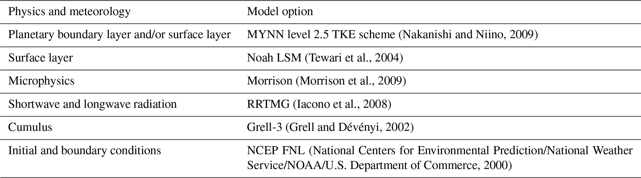

Table A1 WRF model setup.

Table A2 Comparison of the success levels of the standard ratio method (standard) and the improved method (improved) for the evaluation experiment performed for five stations and three tracers. Bold numbers indicate which method scored better.