Chemistry–climate feedback of atmospheric methane in a methane-emission-flux-driven chemistry–climate model

The chemical sink of atmospheric methane (CH₄) depends on the temperature and on the chemical composition. Here, we assess the feedback on atmospheric CH₄ induced by changes in the chemical sink in a warming climate using a CH₄-emission-flux-driven set-up of the chemistry–climate model EMAC (ECHAM/MESSy Atmospheric Chemistry), in which the chemical feedback of CH₄ mixing ratios can evolve explicitly. We perform idealized perturbation simulations driven either by increased carbon dioxide (CO₂) mixing ratios or by increased CH₄ emission fluxes. The CH₄ emission flux perturbation leads to a large increase of CH₄ mixing ratios. Remarkably, the factor by which the CH₄ mixing ratio increases is larger than the increase factor of the emission flux, because the atmospheric lifetime of CH₄ is extended.

In contrast, the individual effect of the global surface air temperature (GSAT) increase is to shorten the CH₄ lifetime, which results in a significant reduction of CH₄ mixing ratios in our set-up. The corresponding radiative feedback is estimated at −0.041 and −0.089 W m⁻² K⁻¹ for the CO₂ and CH₄ perturbation, respectively. The explicit response of CH₄ mixing ratios leads to secondary feedbacks on the hydroxyl radical (OH) and ozone (O₃). Firstly, the OH response includes the CH₄–OH feedback, which enhances the CH₄ lifetime change, and, secondly, the formation of tropospheric O₃ is reduced. Our CH₄ perturbation induces the same response of GSAT per effective radiative forcing (ERF) as the CO₂ perturbation, which supports the applicability of the ERF framework for CH₄.

1 Introduction

Methane (CH₄) is, after carbon dioxide (CO₂), the second most important anthropogenic greenhouse gas (GHG). Compared to CO₂, CH₄ has a larger radiative efficiency (Forster et al., 2021) and a shorter atmospheric lifetime of about 10 years (e.g. Prather et al., 2012; Stevenson et al., 2020). Therefore, reducing atmospheric CH₄ mixing ratios is considered an important measure to mitigate climate change on a decadal timescale (Saunois et al., 2016; Collins et al., 2018; Ocko et al., 2021; Staniaszek et al., 2022). The relatively short atmospheric lifetime of CH₄ is a consequence of the fact that CH₄ is a chemically active species. According to Saunois et al. (2020), the most important sink of atmospheric CH₄ is oxidation by the hydroxyl radical (OH). Thus, understanding the chemical mechanisms underlying CH₄ oxidation is crucial when assessing its climate impact and mitigation options.

Besides its direct radiative effect, indirect contributions from ozone (O₃) and stratospheric water vapour (H₂O) enhance the effective radiative forcing (ERF) of CH₄ (Shindell et al., 2005, 2009; Stevenson et al., 2013; Winterstein et al., 2019; Thornhill et al., 2021b; O'Connor et al., 2022). In addition to its climate impact, tropospheric O₃ poses harmful effects on human health (Nuvolone et al., 2018) and on vegetation (Ashmore, 2005). Therefore, mitigation options involving CH₄ emission reductions have beneficial effects on air quality (Shindell et al., 2012; Staniaszek et al., 2022) and plant productivity (Sitch et al., 2007). In addition to the effects on O₃ and H₂O, CH₄ oxidation reduces OH, which feeds back onto its own atmospheric lifetime (e.g. Winterstein et al., 2019) and affects the rate of formation of secondary aerosols, leading to a shift in the aerosol-size distribution. The latter, in turn, influences aerosol–radiation interactions and aerosol–cloud interactions and is considered another indirect contribution to the ERF of CH₄ (Kurtén et al., 2011; O'Connor et al., 2022).

Next to its importance for indirect contributions to the ERF, CH₄ oxidation largely constrains the atmospheric lifetime of CH₄ and, thus, together with the magnitude of the emissions, its direct radiative effect. The atmospheric lifetime of CH₄ is not constant but depends on the temperature and on the chemical background, which determines the abundance of its sink reactants, especially OH. OH is influenced by a multitude of factors (e.g. Voulgarakis et al., 2013; Stevenson et al., 2020). Among others, meteorological factors such as humidity and temperature influence the abundance of OH. Hence, climate feedbacks of the chemical sink of CH₄ and thereby its lifetime are to be expected. More precisely, the CH₄ lifetime is projected to shorten as a result of tropospheric warming (Voulgarakis et al., 2013; Stecher et al., 2021; Heimann et al., 2020; Thornhill et al., 2021a). To date, only a limited number of studies have assessed the corresponding response of CH₄ mixing ratios directly (Heimann et al., 2020). Even though efforts are ongoing to employ chemistry–climate models (CCMs) in a CH₄-emission-flux-driven model set-up (Shindell et al., 2013; He et al., 2020; Folberth et al., 2022), it is still common practice to prescribe CH₄ mixing ratios at the lower boundary. For instance, the latter method was pursued in the Aerosol Chemistry Model Intercomparison Project (AerChemMIP; Collins et al., 2017), which was endorsed in the Coupled Model Intercomparison Project 6 (CMIP6; Eyring et al., 2016), which, in turn, built the basis for the last report of the Intergovernmental Panel on Climate Change (IPCC, 2021).

When CH₄ mixing ratios are prescribed at the surface, the CH₄ adjustment to changes in the chemical sink is suppressed in the troposphere and can be only derived offline from the atmospheric lifetime change (Dietmüller et al., 2014; Heinze et al., 2019; Thornhill et al., 2021a). This offline method, however, suppresses indirect feedbacks induced by the CH₄ response. Firstly, when CH₄ mixing ratios are free to evolve, the resulting CH₄ response alters the atmospheric CH₄ lifetime, which in turn leads to further changes in the CH₄ mixing ratios. The derivation of the CH₄ response from the lifetime change usually accounts for this effect by including a constant CH₄–OH feedback factor f (Heinze et al., 2019; Thornhill et al., 2021a) so that the equilibrium CH₄ mixing ratio [CH₄]_eq is estimated as (e.g. Stevenson et al., 2020)

$$\begin{array}{}\text{(1)}& [{\mathrm{CH}}_{\mathrm{4}}{]}_{\mathrm{eq}}=[{\mathrm{CH}}_{\mathrm{4}}{]}_{\mathrm{ref}}{\left({\displaystyle \frac{{\mathit{\tau }}_{\exp }}{{\mathit{\tau }}_{\mathrm{ref}}}}\right)}^f,\end{array}$$

where [CH₄]_ref is the reference CH₄ mixing ratio and τ_ref and τ_exp are the reference and perturbed atmospheric lifetimes of CH₄, respectively. Estimates of f are in the range of 1.19 to 1.55 (Fiore et al., 2009; Voulgarakis et al., 2013; Stevenson et al., 2013; Thornhill et al., 2021b; Stevenson et al., 2020; Sand et al., 2023). Holmes (2018) found that f can vary geographically and seasonally and that it strengthens with an increasing CH₄ burden. Secondly, the subsequent CH₄ response affects other chemical constituents such as O₃. This effect is also sometimes accounted for by scaling the sensitivity of O₃ towards CH₄ perturbations with the expected CH₄ response (Fiore et al., 2009; Thornhill et al., 2021b). However, previous studies that assessed the climate feedback of O₃ and the corresponding implication for the global surface air temperature (GSAT) response did not, or only rudimentarily, account for the interaction between changes in O₃ and CH₄ (Dietmüller et al., 2014; Nowack et al., 2015; Marsh et al., 2016; Li and Newman, 2023). As for O₃ alone, the latter studies indicate that its feedback reduces the resulting GSAT response, or in other words that it is a negative feedback. The magnitude of this feedback, however, is highly model dependent.

In this study, we use a CH₄-emission-flux-driven set-up of the CCM ECHAM/MESSy Atmospheric Chemistry (EMAC; Jöckel et al., 2016) to explicitly simulate the response of atmospheric CH₄ mixing ratios resulting from changes in the chemical sink and in CH₄ emissions. We perform idealized perturbation simulations with either increased CO₂ mixing ratios (with CO₂ being an inert GHG) or increased CH₄ emission fluxes. The CH₄ perturbation affects the chemical composition directly, whereas the CO₂ perturbation influences the chemical composition only indirectly, e.g. through the temperature change. From the simulation results we assess the change in CH₄ mixing ratios and its implications for OH and O₃. In addition to the CH₄ feedback, GSAT changes induce other processes that influence O₃. For instance, temperature changes affect chemical reaction rates, emissions of precursor species from natural sources, circulation, or the abundance of H₂O (e.g. Stevenson et al., 2006; Chiodo et al., 2018; Abalos et al., 2020; Griffiths et al., 2021; Zanis et al., 2022). Therefore, we apply an attribution method for O₃ (TAGGING; Grewe et al., 2017; Rieger et al., 2018) to identify and quantify the importance of individual source categories that influence tropospheric O₃ under tropospheric warming.

Our analysis is based on the ERF conceptual framework (Shine et al., 2003; Hansen et al., 2005; Ramaswamy et al., 2018; Forster et al., 2021), which means that the so-called fast and (slow) climate responses are assessed separately. The fast response represents the part of the full response that develops, on short timescales, independently of the corresponding GSAT change, whereas the climate response represents the isolated effect of the GSAT change. There is no formal timescale that separates the fast and slow responses, but they are distinguished conceptually by the dependence on the GSAT response, which is coupled to the (slow) response of the ocean. It is noteworthy that the CH₄ adjustment that follows the increase of CH₄ emission fluxes evolves on the timescale of decades, whereas typical physical (rapid) adjustments evolve on the timescale of weeks or months (e.g. Smith et al., 2018). We derive ERF and the fast response from simulations with prescribed sea surface temperatures (SSTs) and sea ice concentrations (SICs) as recommended by Forster et al. (2016). The climate response is assessed as the difference between the response in a simulation coupled to a mixed layer ocean model and the respective fast response. Analogously, we assess (rapid radiative) adjustments as the radiative effects corresponding to changes in the fast response and (slow climate) feedbacks as the radiative effects corresponding to changes in the climate response.

The paper is structured as follows. Section 2 explains the simulation set-up (Sect. 2.1.), as well as the TAGGING method to attribute O₃ to individual source categories (Sect. 2.2.), and the method to derive the radiative effects corresponding to composition changes in individual species (Sect. 2.3.). Additionally, Sect. 2.3. introduces the theoretical framework for radiative forcing and climate sensitivity. Section 3 presents the simulation results. In Sect. 3.1. and 3.2., we present composition changes in the CO₂ and CH₄ perturbation simulations, respectively. In Sect. 3.3., the corresponding radiative effects are addressed. We conclude with a general discussion and summary of our findings in Sect. 4. Parts of the paper are based on the PhD thesis of the first author (Stecher, 2024).

2 Methods

2.1 Model description and simulation strategy

We use the modular CCM ECHAM/MESSy Atmospheric Chemistry (EMAC; Jöckel et al., 2016) in version 2.55.2. All simulations are performed at a resolution of T42L90MA, i.e. at a triangular (T) truncation at wave number 42 of the spectral dynamical core, corresponding to a quadratic Gaussian grid of approximately 2.8° × 2.8° resolution in latitude and longitude and 90 vertical levels, with the uppermost level centred around 0.01 hPa. The simulations are performed as time slices, which means that the same boundary conditions are repeated cyclically for each simulation year. The boundary conditions, i.e. prescribed emissions and mixing ratios of well-mixed GHGs, represent the year 2010. The quasi-biennial oscillation (QBO) is nudged following the method of Giorgetta and Bengtsson (1999) as described by Jöckel et al. (2016), which introduces some interannual variability. The simulation set-up builds on previous studies assessing the impact of enhanced CH₄ mixing ratios with EMAC (Winterstein et al., 2019; Stecher et al., 2021), with the important advance that for the present study EMAC is used in a CH₄-emission-flux-driven set-up, which means that CH₄ emission fluxes instead of CH₄ mixing ratios are prescribed at the lower boundary. The CH₄ emission fluxes are prescribed as offline emission fluxes; i.e. there are no feedbacks on CH₄ emission fluxes from natural sources such as wetlands or permafrost, which are expected to change in a changing climate (e.g. O'Connor et al., 2010; Dean et al., 2018).

The applied CH₄ emission inventory is an inverse optimized inventory for the EMAC model (Frank, 2018). For the two reference simulations (see Table 1 and text below), monthly mean emissions of the year 2010 are repeated cyclically and scaled by a globally constant factor of 1.08, which corresponds to total annual mean emissions of 625.3 Tg (CH₄) a⁻¹. The scaling was applied to bring the simulated CH₄ surface mixing ratios closer to observations. As the tropospheric mean CH₄ lifetime is about 10 years (e.g. Prather et al., 2012; Stevenson et al., 2020), the CH₄ mixing ratios of the year 2010 result not only from CH₄ emissions of the year 2010, but also from emissions of the years before. Therefore, it cannot be expected that the cyclic repetition of CH₄ emissions of the year 2010 results in CH₄ mixing ratios that represent the year 2010 exactly. Applying the scaling, the resulting global mean CH₄ surface mixing ratio is 1.82 ppmv for both reference simulations. This is in close agreement with observational estimates for the years 2010 and 2012 of 1.80 and 1.81 ppmv by the National Oceanic and Atmospheric Administration Earth System Research Laboratories (NOAA/ESRL) (Lan et al., 2022) and estimates of 1.81 and 1.82 ppmv by the WMO World Data Centre for Greenhouse Gases (WMO, 2022). The estimates of NOAA/ESRL tend to be lower, as only unpolluted marine surface sites contribute to the global estimate. The chemical sink reactions of CH₄ with OH, excited oxygen (O(¹D)) and chlorine (Cl), and CH₄ photolysis are interactively accounted for by the MESSy submodels Module Efficiently Calculating the Chemistry of the Atmosphere (MECCA; Sander et al., 2019) and JVAL (Sander et al., 2014). Oxidation by OH dominates the tropospheric CH₄ sink, so that the reaction with Cl accounts for only 0.23 % of the total chemical tropospheric CH₄ loss (see Table S1 in the Supplement). Therefore, we focus on CH₄ lifetime changes with respect to oxidation by OH. In addition to the sink reactions of CH₄, the chemical mechanism covers the basic chemistry of O₃, OH, hydroperoxyl (HO₂), nitrogen oxides, alkanes and alkenes up to four C atoms, and isoprene (C₅H₈). Further, halogen chemistry of bromine and chlorine species is included. Alkynes, aromatics, and mercury are not considered. In total, the used mechanism covers 265 gas-phase, 82 photolysis, and 12 heterogeneous reactions of 160 species. The chemical feedback on H₂O modifies the prognostic specific humidity, and vice versa. The soil sink of CH₄ is included by the submodel DDEP (Kerkweg et al., 2006a), which uses a prescribed deposition rate (Spahni et al., 2011; Curry, 2007) that is scaled to the actual CH₄ mixing ratio in the corresponding grid box. On average, the global soil sink is 27.6 Tg (CH₄) a⁻¹ for both reference simulations.

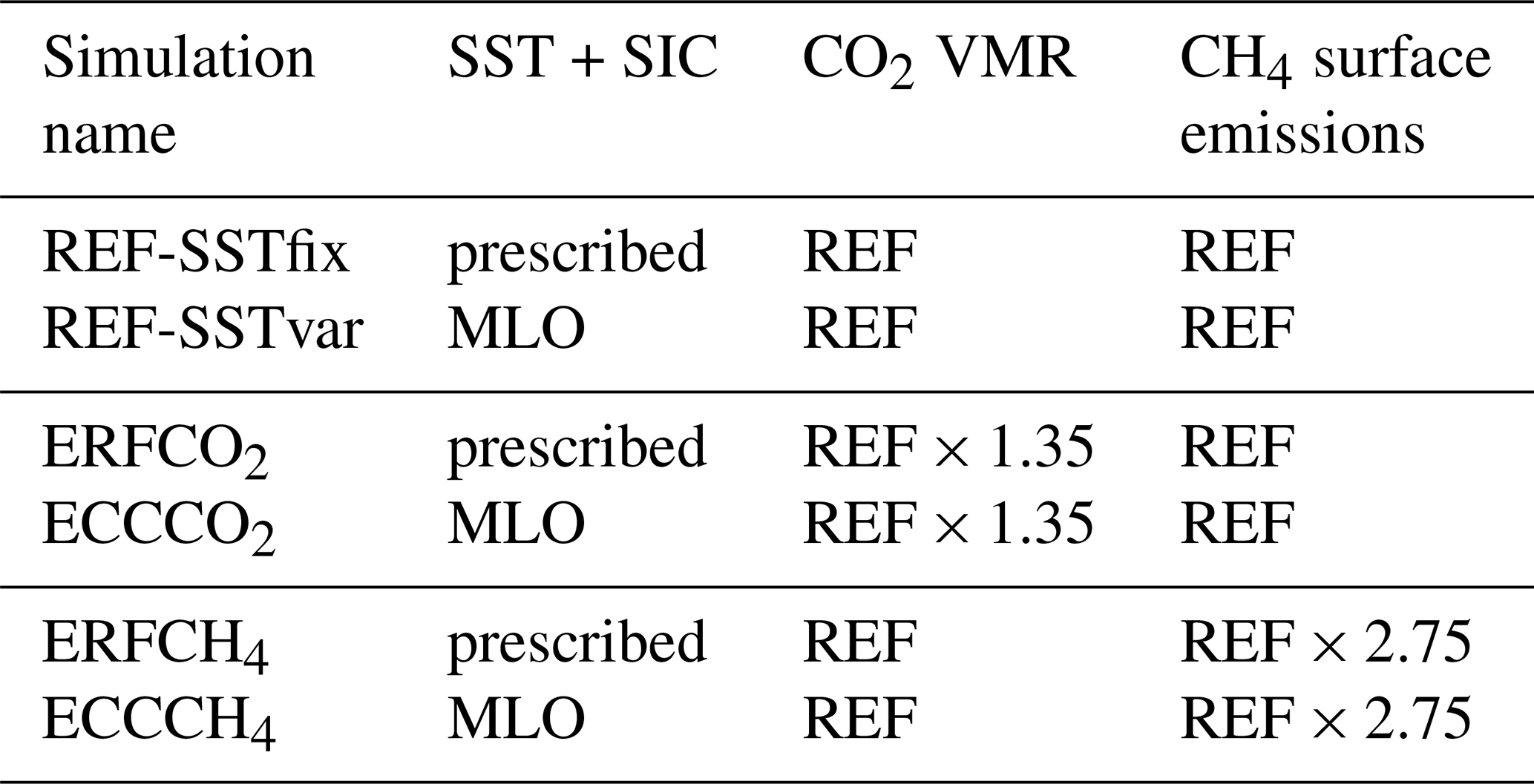
Table 1 Overview of performed simulations. REF indicates that the respective reference is used, which is 388.4 ppmv for the global mean surface mixing ratio of CO₂ and 625.3 Tg (CH₄) a⁻¹ for the CH₄ surface emissions. The prescribed multi-year monthly mean climatology of SSTs and SIC is based on an observation-based estimate of the years 2000 to 2009 from the Met Office Hadley Centre (Rayner et al., 2003).

Precursor emissions of O₃, in particular nitrogen oxides NO and NO₂ (NO_x), non-methane hydrocarbons (NMHCs), and carbon monoxide (CO), are treated as described by Jöckel et al. (2016). Anthropogenic emissions of these species are prescribed from the MACCity inventory (Lamarque et al., 2010; Granier et al., 2011; Diehl et al., 2012), whereby the (mostly monthly resolved) emission fluxes of the year 2010 are repeated cyclically. In addition, climatologies of biogenic emissions of NMHCs and CO are prescribed from the Global Emissions InitiAtive (GEIA). Natural emissions of NO_x from lightning, emissions of NO_x and C₅H₈ from biogenic sources, and the exchange of chemical species between the atmosphere and ocean are parameterized. For lightning NO_x the parameterization of Grewe et al. (2001) is used in the MESSy submodel LNOX (Tost et al., 2007). The 20-year mean global emissions from lightning NO_x are 5.2 Tg (N) a⁻¹ for both reference simulations (see Table 3). Interactive biogenic emissions of soil NO_x and C₅H₈ are calculated by the submodel ONEMIS (Kerkweg et al., 2006b). On average, biogenic NO_x emissions are 6 Tg (N) a⁻¹, and biogenic C₅H₈ emissions are about 307 Tg (C) a⁻¹ for both reference simulations (see Table 3). The atmosphere–ocean exchange of the chemical species C₅H₈, dimethyl sulfide (DMS), and methanol (CH₃OH) is parameterized using the submodel AIRSEA (Pozzer et al., 2006). The mixing ratios of CO₂, nitrous oxide (N₂O), and ozone-depleting substances (ODSs) are prescribed at the lower boundary using monthly mean values of the year 2010 (Meinshausen et al., 2011; Carpenter et al., 2018). For the radiation, a CFC-11 equivalent is calculated lumping additional radiatively active ODSs via radiative efficiencies following the approach by Meinshausen et al. (2017). For the short-lived halocarbons CHCl₂Br, CHClBr₂, and CH₂ClBr, as well as CH₂Br₂ and CHBr₃, surface emissions are prescribed from Warwick et al. (2006) and Liang et al. (2010), respectively.

Table 1 summarizes the performed simulations. The reference simulation with prescribed SSTs and SICs and interactive chemistry (REF-SSTfix) and the reference simulation with MLO and interactive chemistry (REF-SSTvar) serve as references for the experiment simulations and represent year 2010 conditions. REF-SSTfix is performed using prescribed SSTs and SICs, whereas for REF-SSTvar a mixed layer ocean (MLO) model is coupled (MESSy submodel MLOCEAN, Kunze et al., 2014; original ECHAM5 code by Roeckner et al., 1995, described in the ECHAM5 documentation, Chap. 6.3–6.5 in Roeckner et al., 2003). The prescribed multi-year monthly mean climatology of SSTs and SIC is an observation-based estimate of the years 2000 to 2009 from the Met Office Hadley Centre (Rayner et al., 2003). The same climatology was used by Winterstein et al. (2019). Appendix C of Stecher (2024) provides a comparison of the two reference simulations. Overall, the simulation REF-SSTvar reproduces the simulation REF-SSTfix well. The largest differences are in the Southern Hemisphere (SH) polar region, where the MLO model tends to underestimate the sea ice area of the prescribed climatology, which has been noted for a similar application of the MLOCEAN submodel as well (Stecher et al., 2021).

The CO₂ perturbation simulation with prescribed SSTs and SICs and interactive chemistry (ERFCO₂) and the CH₄ perturbation simulation with prescribed SSTs and SICs and interactive chemistry (ERFCH₄) are performed with the same prescribed climatology of SSTs and SICs as REF-SSTfix to assess the so-called fast response and to quantify the ERF and the adjustments following the fixed SST method (e.g. Forster et al., 2016). ERF is defined as the top-of-atmosphere (TOA) net radiative flux change between the experiment and the reference simulation. The perturbations of CO₂ and CH₄ are scaled to result in ERFs of similar magnitude, because for a most fair comparison of the climate sensitivity parameters of different perturbation agents, the respective forcings need to be at the same order of magnitude as the climate sensitivity, as it can be dependent on the magnitude of the forcing (e.g. Hansen et al., 2005; Dietmüller et al., 2014). The ERF is targeted to be large enough to cause statistically significant and interpretable feedbacks (Forster et al., 2016) and small enough to be reached with still realistically large perturbations of CO₂ and CH₄ (Dietmüller et al., 2014; Winterstein et al., 2019). Perturbations of 1.35 × CO₂ mixing ratios and 2.75 × CH₄ surface emission fluxes result in ERFs of 1.61 ± 0.16 and 1.72 ± 0.17 W m⁻², respectively (see Table 4). The scaling of 1.35 × CO₂ mixing ratios or 2.75 × CH₄ surface emission fluxes is applied to all CO₂ and CH₄ perturbation experiments, respectively. The CO₂ perturbation simulation with MLO and interactive chemistry (ECCCO₂) and the CH₄ perturbation simulation with MLO and interactive chemistry (ECCCH₄) are so-called equilibrium climate change simulations. In these simulations the MLO model accounts for the response of SSTs and SICs. Therefore, the effect of GSAT-driven feedbacks is included in these simulations.

In the following, we assess the so-called fast response as the difference between ERFCO₂ or ERFCH₄ and REF-SSTfix, as well as the full response as the difference between ECCCO₂ or ECCCH₄ and REF-SSTvar. The difference between the full and the fast response is assessed as the climate response, which represents the isolated effect of the GSAT change. Similarly, adjustments and feedbacks are defined as the radiative effects corresponding to the fast response and the climate response, respectively. For the analysis, results of 20 simulated years after the spin-up period are used. The spin-up ensures that a quasi-equilibrium is reached and is, therefore, different for the individual simulations according to the simulation set-up. For ERFCH₄ the longest spin-up period of 90 years was necessary; for ECCCO₂ and ECCCH₄ a period of 50 years was necessary, respectively; and for ERFCO₂ a period of 25 years was necessary. Time series of the global mean surface CH₄, the total atmospheric masses of CH₄ and O₃, the TOA radiation balance, and GSAT (for the MLO simulations) were monitored to decide whether an equilibrium is reached. In addition, we assessed the spin-up of the mass of CH₄ of the simulation ERFCH₄ in more detail. A curve fit was applied to the spin-up period to derive the atmospheric mass of CH₄ in equilibrium. The mass of CH₄ follows the exponential function of the form $a-b\cdot \exp (-t/c)$ closely. The mass of CH₄ in the last year of the spin-up, simulation year 90, is about 0.5 % smaller than the derived equilibrium estimate (parameter a) and therefore spun-up sufficiently well (see Fig. S14). The derived perturbation lifetime (parameter c) is 21.6 years. We note that the perturbation lifetime is larger than that of the CH₄ emission reduction experiment by Staniaszek et al. (2022). As the perturbation lifetime increases with increasing CH₄ burden (Holmes, 2018), this can be expected. In addition, model differences and the magnitude of the emission change might play a role.

In this study, the CH₄ lifetime is calculated according to Jöckel et al. (2016) as

$$\begin{array}{}\text{(2)}& {\mathit{\tau }}_{{\mathrm{CH}}_{\mathrm{4}}}={\displaystyle \frac{\sum _{b\in B}{m}_{{\mathrm{CH}}_{\mathrm{4}}}}{\sum _{b\in B}{k}_{{\mathrm{CH}}_{\mathrm{4}}+\mathrm{OH}}\left(T\right)\cdot c_{\mathrm{air}}(T,p,q)\cdot x_{\mathrm{OH}}\cdot m_{{\mathrm{CH}}_{\mathrm{4}}}}},\end{array}$$

with $m_{{\mathrm{CH}}_{\mathrm{4}}}$ being the mass of CH₄ in kilograms (kg), $k_{{\mathrm{CH}}_{\mathrm{4}}+\mathrm{OH}}\left(T\right)$ being the temperature (T)-dependent reaction rate coefficient of the reaction ${\mathrm{CH}}_{\mathrm{4}}+\mathrm{OH}\to \mathrm{products}$ in cm³ s⁻¹, c_air being the concentration of air in cm⁻³, and x_OH being the mole fraction of OH in mol mol⁻¹ in all grid boxes b∈B. B is the region for which the lifetime should be calculated, e.g. all grid boxes below the tropopause for the mean tropospheric lifetime. For the CH₄ lifetime calculation a climatological tropopause, defined as tp_clim=300–215 hPa ⋅cos ²(ϕ), with ϕ being the latitude in degrees north, is used as recommended by Lawrence et al. (2001). The reaction rate coefficient $k_{{\mathrm{CH}}_{\mathrm{4}}+\mathrm{OH}}\left(T\right)$ is calculated as in the applied kinetic equation system (submodel MECCA), i.e. as

$$\begin{array}{}\text{(3)}& k_{{\mathrm{CH}}_{\mathrm{4}}+\mathrm{OH}}\left(T\right)=\mathrm{1.85}\times {\mathrm{10}}^{-\mathrm{20}}\cdot T^{\mathrm{2.82}}\cdot \exp \left(-{\displaystyle \frac{\mathrm{987}}{T}}\right).\end{array}$$

2.2 TAGGING

The TAGGING method (Grewe et al., 2017; Rieger et al., 2018) quantifies the contributions of individual source categories to the mixing ratios of tagged tracers. Tagged tracers are O₃, CO, reactive nitrogen compounds (NO_y), peroxyacyl nitrate (PAN), NMHCs, OH, and HO₂. For computational reasons NMHCs and NO_y are considered with a family approach. For these species or families of species, the individual contributions of emission categories or source processes are calculated. In this study O₃ production from the following categories is considered:

• through photolysis of molecular oxygen (O₂) in the stratosphere (O₃ stratosphere);

• from emissions of lightning NO_x (O₃ lightning);

• from biogenic precursor emissions, mainly soil NO_x and C₅H₈ (O₃ biogenic);

• from products of the CH₄ decomposition (O₃ CH₄);

• from products of the N₂O decomposition (O₃ N₂O);

• from biomass burning precursor emissions (O₃ biomass burning); and

• from anthropogenic precursor emissions (O₃ anthropogenic).

The categories are the same as defined by Grewe et al. (2017), except for the category O₃ anthropogenic, which, in our study, combines O₃ production from all anthropogenic emissions, i.e. of the sectors industry, road traffic, shipping, and aviation.

The tagged tracers (i.e. the individual contributions) undergo the same processes as the corresponding total species. These are transport, emissions, dry and wet deposition, and chemical production and loss (see Grewe et al., 2017, for details). For the short-lived species OH and HO₂ a steady state between chemical production and loss is assumed (Rieger et al., 2018). The chemical reaction rates are taken from the submodel MECCA. Effective production and loss are taken into account for O₃, meaning that production and loss terms from a family, which includes all fast exchanges between O₃ and other chemical species, are considered. The diagnostic tool ProdLoss (Grewe et al., 2017) is used to identify all reactions that contribute to effective O₃ production and loss in the applied chemical mechanism. The reaction rates of effective O₃ production and loss are then manually grouped into O₃ production and loss rates, depending on which tagged species contributes to O₃ production or loss.

2.3 Quantification of individual radiative effects

The assessment of radiative effects in this study follows the ERF framework. This means that (rapid radiative) adjustments, which are defined as the TOA net radiative flux change corresponding to changes in the fast response, i.e. independent from GSAT changes, are accounted for as part of the forcing. Thus, ERF is given as the sum of instantaneous radiative forcing (IRF), defined as the net radiative flux change at TOA excluding any adjustment, and the sum of all individual adjustments A_i (e.g. Smith et al., 2018):

$$\begin{array}{}\text{(4)}& \mathrm{ERF}=\mathrm{IRF}+\sum _i{A}_i.\end{array}$$

Consistently, (slow climate) feedbacks are defined as the TOA net radiative flux change induced by atmospheric parameter changes that correspond to the gradually changing GSAT. These feedbacks act to reduce or enhance the associated GSAT change (ΔT) and determine the climate sensitivity parameter λ (units: K (W m⁻²)⁻¹), which is the proportionality constant that relates the equilibrium change in GSAT to the ERF as

$$\begin{array}{}\text{(5)}& \mathrm{\Delta }T=\mathit{\lambda }\cdot \mathrm{ERF}.\end{array}$$

The feedback parameter α is the negative inverse of the climate sensitivity parameter λ ($\mathit{\alpha }=-\mathrm{1}/\mathit{\lambda }$; units: W m⁻² K⁻¹). The feedback parameter quantifies the net radiative flux change at TOA for a given change in GSAT. Under the assumption of linearity it can be decomposed into the radiative contributions of individual processes affected by the change in GSAT, i.e. the individual feedback parameters α_i, so that (e.g. Forster et al., 2021)

$$\begin{array}{}\text{(6)}& \mathit{\alpha }=\sum _i{\mathit{\alpha }}_i=\sum _i{\displaystyle \frac{\partial N}{\partial x_i}}{\displaystyle \frac{\mathrm{d}{x}_i}{\mathrm{d}T}},\end{array}$$

where N is the radiative flux change at TOA induced by the change in an individual variable of the Earth system x_i.

We quantify adjustments and feedbacks corresponding to composition changes in CO₂, CH₄, O₃, and stratospheric H₂O following the method used by Winterstein et al. (2019) and Stecher et al. (2021). Additional simulations are performed with EMAC using the option for multiple diagnostic radiation calls (Dietmüller et al., 2016; Nützel et al., 2024). These simulations are performed (for the sake of saving computational resources) without interactive chemistry but with prescribed climatologies for the radiatively active trace gases CH₄, CO₂, O₃, N₂O, and the chlorofluorocarbons (CFCs) from the simulations REF-SSTfix or REF-SSTvar. SSTs and SICs are prescribed using the same observation-based climatology as used for REF-SSTfix (Rayner et al., 2003). Thus, the background climate of the simulations represents reference conditions. The additional simulations are run over 2 years each (plus 1-year spin-up).

In these simulations the first radiation call, P, provides the radiative heating rates that drive the base model, whereas the other radiation calls, D1, D2, etc., are purely diagnostic. The radiation call D1 serves as the reference for the perturbations and receives identical input as P, except for the specific humidity, for which a monthly mean climatology from the respective reference simulation (REF-SSTfix or REF-SSTvar) is used instead of the prognostic specific humidity from the base model. This is necessary because the radiation calls to calculate the radiative effect of H₂O use monthly mean climatologies of the specific humidity from the sensitivity simulations (see below) and therefore need to be compared to a radiation call, which uses a monthly mean climatology of specific humidity instead of the prognostic, highly variable, specific humidity.

In the other radiation calls (D2, D3, etc.) either CO₂, CH₄, O₃, or the specific humidity is replaced by a monthly mean climatology from the sensitivity simulation (either ERFCO₂, ECCCO₂, ERFCH₄, or ECCCH₄) to calculate the corresponding radiative effect. For example, to derive the radiative effect of the full response of CH₄ of the CO₂ perturbation, the reference CH₄ climatology in D1 is replaced by the monthly mean CH₄ climatology from ECCCO₂ in D2. For O₃ and the specific humidity, the radiative effects of changes in the troposphere and in the stratosphere are derived separately. The diagnostic radiation calls include the stratospheric temperature adjustment induced by the respective perturbation following the method of Stuber et al. (2001). Therefore, the radiative effect corresponding to CH₄ (CO₂) from the simulation ERFCH₄ (ERFCO₂) represents stratospheric-temperature-adjusted radiative forcing (SARF), i.e. the direct radiative effect of the perturbation including the associated stratospheric temperature adjustment. To define the region in which the stratospheric temperature adjustment is applied, as well as to separate tropospheric and stratospheric radiative effects of O₃ and the specific humidity, the climatological tropopause tp_clim is used consistently with the CH₄ lifetime calculation (see Sect. 2.1).

There is one methodological difference compared to Winterstein et al. (2019) and Stecher et al. (2021). They used the climatological specified humidity directly in the first prognostic radiation call, which then served as the reference for the perturbed calls. However, here it was decided to use the prognostic specific humidity in the first radiation call as it is consistent with the model's background meteorology, e.g. the cloud cover. The influence on the calculated radiative effects was tested and found to be up to 1.02 % (or 0.004 W m⁻²), with the maximum deviation for the perturbations of specific humidity, which is negligible in comparison to other uncertainties.

3 Results

3.1 Methane and ozone composition changes following 1.35 × CO₂ perturbation

In this section, we present the simulation results of the 1.35 × CO₂ perturbation. Figure 1 shows the annual zonal mean composition changes in CH₄ mixing ratios in the simulations ERFCO₂ (fast response) and ECCCO₂ (full response), as well as their difference, which is interpreted as the climate response. The fast response is dominated by increasing CH₄ mixing ratios in the upper stratosphere and mesosphere. In this region, the cooling to be expected from the CO₂ increase (see Fig. S1 in the Supplement) leads to the prolongation of the CH₄ lifetime. The stratospheric CH₄ loss by reaction with OH, Cl, and O(¹D) is reduced by about 2 % (see Table S1 in the Supplement). A similar effect has been noted by Dietmüller et al. (2014). In the fast response, tropospheric CH₄ shows a slight increase below 2 %.

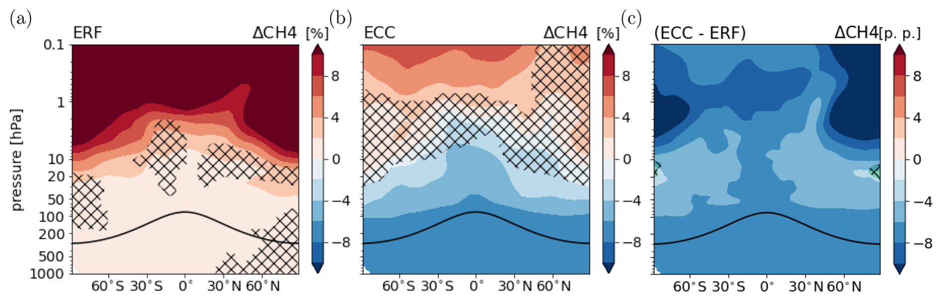
Figure 1 CH₄ response following the CO₂ perturbation. Relative differences between the annual zonal mean CH₄ mixing ratios of sensitivity simulations (a) ERFCO₂ (fast response) and (b) ECCCO₂ (full response) and their respective reference simulation in percent (%). (c) Climate response as the difference between the CH₄ responses in panels (a) and (b) in percentage points (p.p.). Non-hatched areas are significant at the 95 % confidence level according to a Welch test based on annual mean values. The solid black line indicates the location of the climatological tropopause.

In contrast to the fast response, the full response shows a significant reduction of CH₄ mixing ratios in the troposphere and lower stratosphere. As CH₄ emission fluxes are prescribed in the simulation set-up and cannot respond to changes in meteorology or composition, any feedback on natural CH₄ emissions (e.g. Dean et al., 2018) is suppressed. Therefore, the decrease of CH₄ mixing ratios results from enhanced chemical decomposition of CH₄, mainly by the oxidation with OH. The tropospheric CH₄ lifetime with respect to oxidation by OH shortens by about 7 months (0.56 a or 7.4 %; see Table 2). This shortening is a combined result of the direct influence of the temperature on the reaction rate coefficient and of an enhanced abundance of OH. Tropospheric warming increases OH mixing ratios throughout the troposphere, with the maximum increase in the tropics (see Fig. S3 in the Supplement). Firstly, emissions from lightning NO_x increase by about 0.3 Tg (N) a⁻¹ in the climate response (see Table 3), which leads to enhanced production of OH. To estimate the effect on the CH₄ lifetime, we use the multi-model mean sensitivity of the CH₄ lifetime towards changing lightning NO_x emissions of −4.8 % (Tg (N) a⁻¹)⁻¹ from Thornhill et al. (2021a), which suggest a shortening of the CH₄ lifetime due to lightning NO_x emissions by 1.4 %. Additionally, the increase in the tropospheric humidity associated with higher temperatures leads to enhanced production of OH.

Table 2 Global annual mean values of tropospheric CH₄ lifetime with respect to oxidation by OH, as well as CH₄ surface volume mixing ratio for the performed simulations.

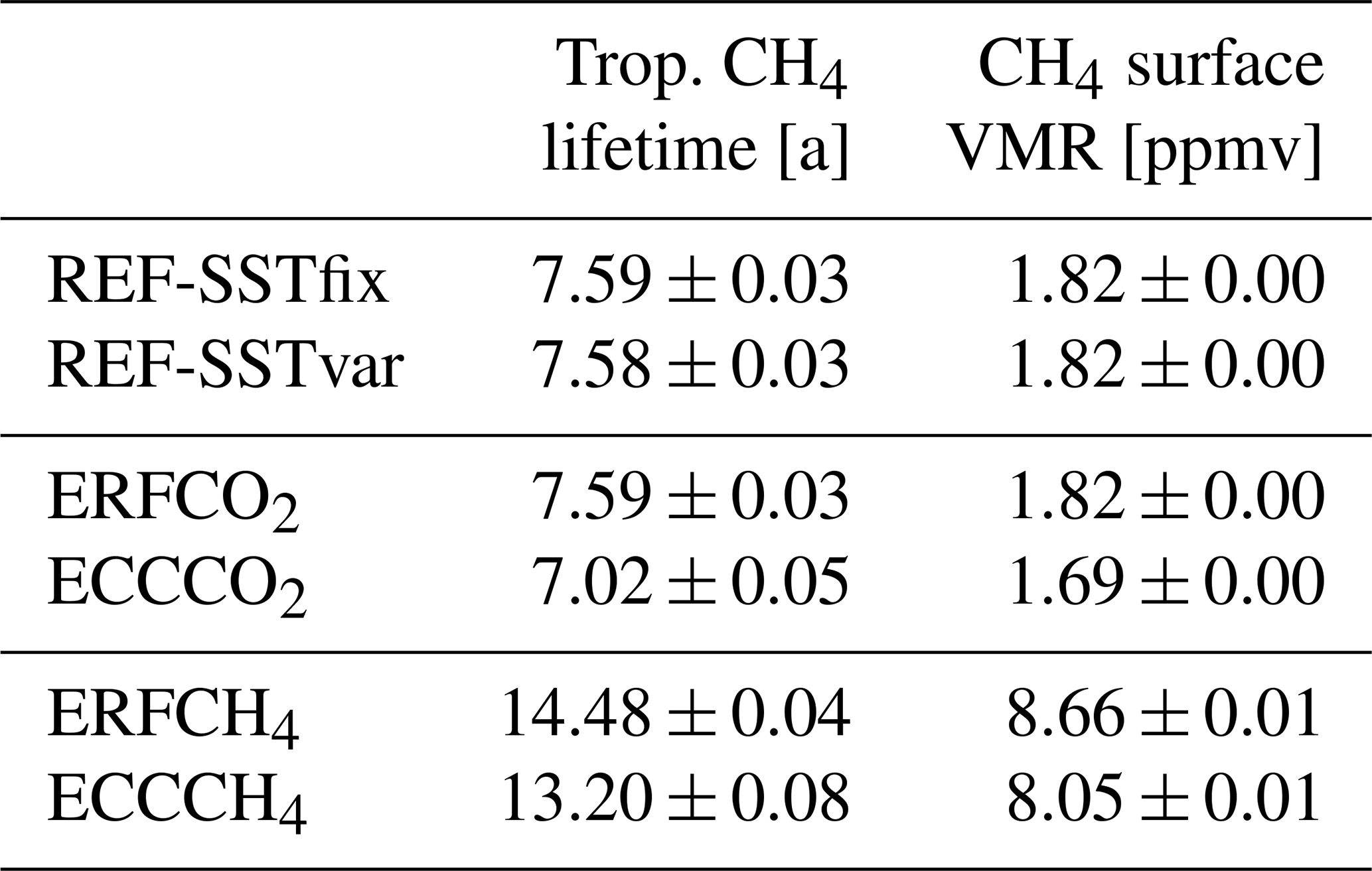
The values after the ± are the corresponding interannual standard deviations based on 20 annual mean values, which are listed to estimate the year-to-year variability.

Table 3 Global annual mean emissions of NO_x from lightning, NO_x from biogenic sources, and C₅H₈ from biogenic sources.

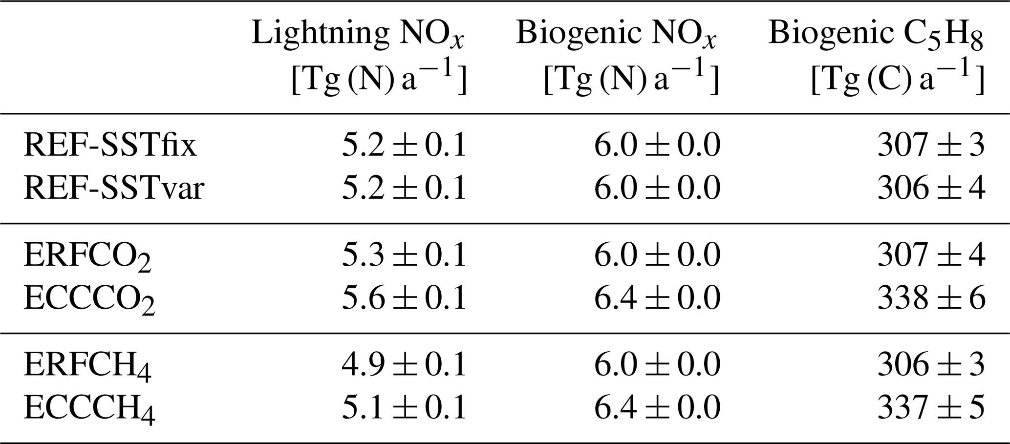
The values after the ± are the corresponding interannual standard deviations based on 20 annual mean values, which are listed to estimate the year-to-year variability. The model-calculated biogenic C₅H₈ emissions are scaled by a factor of 0.6 before being added to the atmospheric C₅H₈ tracer (see Jöckel et al., 2016). The values shown here include the scaling.

In addition to the reduction in the troposphere, the CH₄ mixing ratios decrease also in the lower stratosphere as part of the full response. As the reaction partners of CH₄, namely OH, Cl, and O(¹D), do not show any significant response in the lower stratosphere (see Fig. S3 for OH) and the stratospheric CH₄ loss does not change (see Table S1 in the Supplement), the decrease is likely a transport effect. Tropospheric air masses with reduced CH₄ mixing ratios compared to the reference simulation enter the stratosphere by the upwelling branch of the Brewer–Dobson circulation. Tropical upwelling is enhanced in the climate response (see Fig. S13 in the Supplement). Dietmüller et al. (2014) noted an increase of CH₄ mixing ratios throughout the stratosphere as a result of 2 × CO₂ due to stratospheric cooling and thereby a slower CH₄ oxidation. In addition, enhanced tropical upwelling transports CH₄ enriched air in the stratosphere more efficiently. In our set-up, the reduction of tropospheric CH₄, which is suppressed in the set-up of Dietmüller et al. (2014) as CH₄ mixing ratios are prescribed at the lower boundary, dominates the latter two processes.

Previous studies also found that tropospheric warming leads to increasing OH mixing ratios and correspondingly to the shortening of the CH₄ lifetime (e.g. Voulgarakis et al., 2013; Dietmüller et al., 2014; Heimann et al., 2020; Stecher et al., 2021; Thornhill et al., 2021a). The novelty of our study is that the associated reduction of CH₄ mixing ratios is simulated explicitly, which was assessed by only a small number of studies so far (Heimann et al., 2020). In our CO₂ perturbation experiment, the CH₄ lifetime change per unit change in GSAT is −0.51 a K⁻¹ or −6.7 % K⁻¹.

Voulgarakis et al. (2013) addressed the sensitivity of the CH₄ lifetime towards climate change in the Atmospheric Chemistry and Climate Model Intercomparison Project (ACCMIP) model ensemble. In the respective sensitivity simulations the boundary conditions for SSTs, SICs, and CO₂ were set to RCP8.5 conditions for the year 2030 or the year 2100, while all other boundary conditions were representative of the year 2000. They found sensitivities of the tropospheric CH₄ lifetime of −0.31 ± 0.14 a K⁻¹ (−3.2 ± 1.0 % K⁻¹) and −0.34 ± 0.12 a K⁻¹ (−3.4 ± 0.8 % K⁻¹) for the year 2030 and the year 2100 experiments, respectively¹. The CMIP6 AerChemMIP model ensemble as analysed by Thornhill et al. (2021a) suggests a sensitivity of the whole-atmosphere CH₄ lifetime towards climate change of −0.6 ± 4.5 % K⁻¹ assessed from abrupt 4 × pre-industrial CO₂ experiments. The large intermodel spread results from one model that shows an extension of CH₄ lifetime as a result to 4 × CO₂. The three models showing a shortening of CH₄ lifetime suggest a sensitivity of −3.2 ± 0.8 % K⁻¹ in close agreement with Voulgarakis et al. (2013).

Our study indicates a larger sensitivity of the CH₄ lifetime towards climate change compared to Voulgarakis et al. (2013) and Thornhill et al. (2021a). Possible reasons are the different magnitudes of the perturbations, differences in the simulation set-ups, or the explicit treatment of the CH₄ feedback in our study. The similar estimates for the years 2030 and 2100, corresponding to 1.14 and 4.76 K change in GSAT, respectively², by Voulgarakis et al. (2013) suggest that the sensitivity is not highly dependent on the magnitude of the perturbation. Furthermore, the set-ups of individual models in Voulgarakis et al. (2013) and Thornhill et al. (2021a) differ, e.g. with respect to the level of complexity of the chemical mechanism, whether interactive aerosol is used, or through the different treatment of natural O₃ precursor emissions. Nevertheless, the present estimate is larger than the estimates of all individual models in Voulgarakis et al. (2013) and Thornhill et al. (2021a), except for two models which do not parameterize the effect of stratospheric O₃ on photolysis rates below, which is taken into account here. In the simulation set-ups analysed by Voulgarakis et al. (2013) and Thornhill et al. (2021a) CH₄ mixing ratios are prescribed at the lower boundary in all models, except for the GISS-E2-R model analysed by Voulgarakis et al. (2013). The lifetime response per unit temperature change derived from GISS-E2-R is comparably weak. GISS-E2-R calculates wetland emissions of CH₄ online, presumably also for the climate sensitivity experiments, which makes it difficult to compare the CH₄ lifetime response in this model to our study. Nevertheless, compared to the other models, the explicit treatment of the CH₄ feedback in our set-up allows for a subsequent feedback on OH and correspondingly for a self-feedback on the CH₄ lifetime, which can explain the enhanced sensitivity of the CH₄ lifetime towards climate change.

If the CH₄ mixing ratio cannot adapt to changes in its lifetime, the corresponding CH₄ equilibrium mixing ratio can be estimated using Eq. (1). The feedback factor f in the equation accounts for the CH₄–OH feedback. In our CH₄-emission-driven simulation the CH₄–OH feedback is implicitly included in the simulated response of OH and the CH₄ lifetime, so that using Eq. (1) with f > 1 applies the CH₄–OH feedback twice in this case. Equation (1) indicates a global mean CH₄ equilibrium mixing ratio in the range of 1.61 to 1.66 ppmv for $f=[\mathrm{1.19},\mathrm{1.55}]$ for the present changes in the CH₄ lifetime. Thus, it suggests a larger reduction than simulated by the model, which adjusts to a global mean CH₄ equilibrium mixing ratio of 1.69 ppmv (see Table 2). However, if the feedback factor is not applied (f = 1), Eq. (1) gives 1.68 ppmv, which is in close agreement with the simulated response of CH₄ mixing ratios.

Figure 2 Same as Fig. 1 but for O₃.

The corresponding response of O₃ is shown in Fig. 2. The fast response is dominated by O₃ increases of up to 8 % in the middle and upper stratosphere. In these regions, CO₂-induced stratospheric cooling causes slower chemical O₃ depletion (e.g. Rind et al., 1998; Rosenfield et al., 2002; Portmann and Solomon, 2007; Dietmüller et al., 2014; Chiodo et al., 2018). In the lowermost stratosphere, O₃ mixing ratios decrease by up to 4 %. This decrease can be explained by the so-called reversed self-healing (Rosenfield et al., 2002; Portmann and Solomon, 2007), which describes the effect that increasing O₃ above leads to a reduction of ultraviolet radiation that reaches the lower stratosphere and consequently to reduced photochemical production of O₃. The effect of transport from the troposphere into the stratosphere is expected to play a minor role in the fast response, as the strength of tropical upwelling is largely determined by the response of SSTs (Garny et al., 2011; Butchart, 2014). The fast response of tropospheric O₃ is smaller than 2 %.

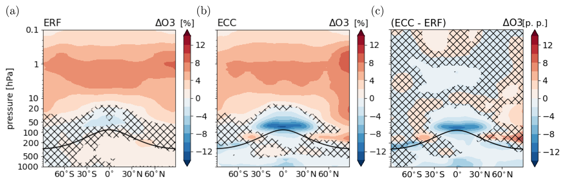
The climate response of O₃ is dominated by a reduction of up to 10 % in the lowermost tropical stratosphere (see Fig. 2c). Enhanced tropical upwelling transports tropospheric O₃ poor air from the troposphere into the stratosphere more efficiently. This is a robust feature across CCMs (Dietmüller et al., 2014; Nowack et al., 2015; Marsh et al., 2016; Chiodo et al., 2018). In the troposphere, O₃ mixing ratios decrease by up to 6 % in the tropics close to the surface and decrease slightly in the upper tropical troposphere.

The pattern of the full response of stratospheric O₃ is qualitatively consistent with previous studies of O₃ changes resulting from a CO₂ perturbation (Dietmüller et al., 2014; Nowack et al., 2015; Marsh et al., 2016; Nowack et al., 2018; Chiodo et al., 2018; Thornhill et al., 2021a). However, the tropospheric response is different here. Most studies using various CCMs consistently show an increase of O₃ in the tropical upper troposphere as part of the full response (Dietmüller et al., 2014; Nowack et al., 2015; Marsh et al., 2016; Nowack et al., 2018; Chiodo et al., 2018). In the studies by Dietmüller et al. (2014) and Nowack et al. (2015, 2018), and presumably also in the studies by Marsh et al. (2016) and Chiodo et al. (2018), CH₄ mixing ratios are prescribed at the lower boundary. Consequently, the negative CH₄ feedback as discussed above cannot evolve. This can lead to an overestimation of O₃ produced from products of the CH₄ oxidation and is consistent with the positive response of O₃ in the upper tropical troposphere. In particular, the comparison with the study by Dietmüller et al. (2014) indicates an effect of the CH₄ feedback on O₃ because the EMAC model was used as well in that study.

Using the MESSy submodel TAGGING (Grewe et al., 2017; Rieger et al., 2018) the tropospheric O₃ response is attributed to individual source categories representing different processes of O₃ production. Consistent with the small fast response of total tropospheric O₃ (Fig. 2a), the corresponding response of the individual categories is below 0.5 % of the total reference O₃ for all categories, except for O₃ stratosphere (see Fig. S5 in the Supplement). The response of the category O₃ stratosphere confirms that less O₃ is produced via photolysis in the lower tropical stratosphere. Additionally, it indicates enhanced transport from the stratosphere into the troposphere in middle and higher latitudes of the Northern Hemisphere (NH).

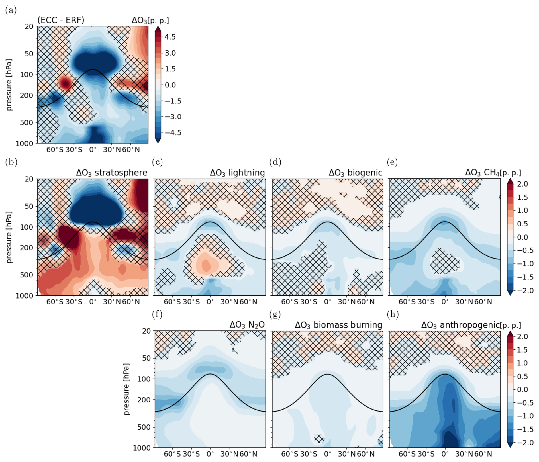
Figure 3 Climate response of tropospheric O₃ following the CO₂ perturbation: (a) response of total O₃ (same as Fig. 2c but with differently scaled colour levels to better compare with the response in the individual source categories), (b–h) response of O₃ in individual categories relative to total reference O₃ $\left(\mathrm{\Delta }{\mathrm{O}}_{{\mathrm{3}}_{\mathrm{cat},\mathrm{climateresponse}}}=\left(\frac{{\mathrm{O}}_{{\mathrm{3}}_{\mathrm{cat},\mathrm{ECC}}}-{\mathrm{O}}_{{\mathrm{3}}_{\mathrm{cat},\mathrm{REF}}}}{{\mathrm{O}}_{{\mathrm{3}}_{\mathrm{total},\mathrm{REF}}}}\right)-\left(\frac{{\mathrm{O}}_{{\mathrm{3}}_{\mathrm{cat},\mathrm{ERF}}}-{\mathrm{O}}_{{\mathrm{3}}_{\mathrm{cat},\mathrm{REF}}}}{{\mathrm{O}}_{{\mathrm{3}}_{\mathrm{total},\mathrm{REF}}}}\right)\right)$. Non-hatched areas are significant at the 95 % confidence level according to a Welch test based on annual mean values. The solid black line indicates the location of the climatological tropopause.

Figure 3 shows the climate response of individual O₃ source categories presented as the difference between the fast and full response of each category in percentage points (p.p.):

$$\begin{array}{}\text{(7)}& \begin{array}{rl}& \mathrm{\Delta }{\mathrm{O}}_{{\mathrm{3}}_{\mathrm{cat},\mathrm{climateresponse}}}=\\ & \left({\displaystyle \frac{{\mathrm{O}}_{{\mathrm{3}}_{\mathrm{cat},\mathrm{ECC}}}-{\mathrm{O}}_{{\mathrm{3}}_{\mathrm{cat},\mathrm{REF}}}}{{\mathrm{O}}_{{\mathrm{3}}_{\mathrm{total},\mathrm{REF}}}}}\right)-\left({\displaystyle \frac{{\mathrm{O}}_{{\mathrm{3}}_{\mathrm{cat},\mathrm{ERF}}}-{\mathrm{O}}_{{\mathrm{3}}_{\mathrm{cat},\mathrm{REF}}}}{{\mathrm{O}}_{{\mathrm{3}}_{\mathrm{total},\mathrm{REF}}}}}\right).\end{array}\end{array}$$

The presentation relative to the total reference O₃ allows the direct comparison of the responses of the individual categories to the relative response of total O₃ as shown in Figs. 2c and 3a.

The climate response of the category O₃ stratosphere shows significantly enhanced transport of stratospheric O₃ into the troposphere in both hemispheres. In the extratropical middle troposphere, O₃ mixing ratios increase by up to 1.5 % relative to the total reference O₃ in the full response, which is the largest positive contribution to the total tropospheric O₃ response. This supports current knowledge, as enhanced entry of stratospheric O₃ under increasing GHG concentrations has been a robust feature in CCMs (Abalos et al., 2020). The category O₃ stratosphere is also the largest contributor to the strong reduction in the lowermost stratosphere. The category O₃ lightning shows a significant increase of up to 1.25 % relative to total reference O₃ in the middle tropical troposphere. This is consistent with an increase of lightning NO_x emissions by about 0.3 Tg (N) a⁻¹ globally (see Table 3). Lightning NO_x is emitted mainly in the upper tropical troposphere where convection is strongest (not shown). Biogenic emissions of NO_x and C₅H₈ increase in the full response as well. Biogenic C₅H₈ emissions increase the most in the Amazon region and the Congo River basin, whereas biogenic NO_x emissions increase over land in the tropics and mid-latitudes (not shown). However, the zonal mean climate response of O₃ biogenic is mostly not significant due to competing effects of enhanced precursor emissions and of enhanced chemical loss with H₂O. An enhanced sink of O₃ via the reaction of O(¹D) with H₂O, which leads to effective O₃ loss, is expected in a warmer and moister troposphere (e.g. Stevenson et al., 2006). The spatial distribution of the tropospheric O₃ column shows mainly a reduction over the tropical ocean (see Fig. S7 in the Supplement), which is also reflected by the significant reduction between the Equator and 30° N in the zonal mean (Fig. 3d). Locally over regions with increasing precursor emissions, e.g. over the Amazon region and the Congo River basin, the tropospheric O₃ column increases in the category O₃ biogenic (see Fig. S7 in the Supplement). Anthropogenic and biomass burning emissions are prescribed and are therefore not affected by the CO₂ increase. In these categories, decreasing O₃ from enhanced loss or reduced O₃ production efficiency is shown. The reduction of O₃ anthropogenic is most pronounced over the tropical ocean, where a decline of O₃ due to enhanced loss via H₂O is expected (Stevenson et al., 2006; Zanis et al., 2022). The effect of the reduction of O₃ biomass burning on total O₃ is small, since also its absolute contribution is small. In addition to the enhanced sink, reduced O₃ production per emitted NO_x could play a role in the latter two categories as O₃ precursor emissions from natural categories increase. The category O₃ CH₄ shows a reduction throughout the troposphere. This is consistent with the reduction of CH₄ mixing ratios, as in the new equilibrium fewer products of the CH₄ oxidation are available for O₃ production, resulting in reduced O₃ production in this category. Further, enhanced chemical loss can contribute to the reduction of this category. In the upper tropical troposphere the increase of lightning NO_x emissions counteracts the effect of the CH₄ decrease by providing enhanced levels of NO_x, which react with the products of the CH₄ oxidation more efficiently. The climate response of O₃ CH₄ is not significant in this region. The climate response in the category O₃ N₂O shows significant decreases in the lower stratosphere and troposphere. In the stratosphere, N₂O mixing ratios increase (not shown) indicating less N₂O decomposition (Dietmüller et al., 2014). Thereby, less nitrogen oxide (NO) is produced to form O₃, which is consistent with the decrease of O₃ formed from N₂O decomposition.

3.2 Methane and ozone composition changes following 2.75 × CH₄ emission flux perturbation

In this section, we present the simulation results of the 2.75 × CH₄ emission flux perturbation. Figure 4 shows the zonal mean distribution of CH₄ mixing ratios of the reference simulation REF-SSTfix and of the two simulations with CH₄ emission fluxes increased by a globally constant factor of 2.75. As expected, CH₄ mixing ratios increase everywhere in the fast response shown in Fig. 4b. Hereby, the increase factor of CH₄ mixing ratios is even larger than the increase factor of the emission fluxes. Table 2 shows that an increase of CH₄ emissions by a factor of 2.75 results in an increase of the global mean surface CH₄ mixing ratio by a factor of 4.76. This is caused by a large extension of the tropospheric CH₄ lifetime by about 7 years (see Table 2). The CH₄ increase reduces the tropospheric OH mixing ratios by up to 60 % (see Fig. S3 in the Supplement), thereby extending the CH₄ lifetime.

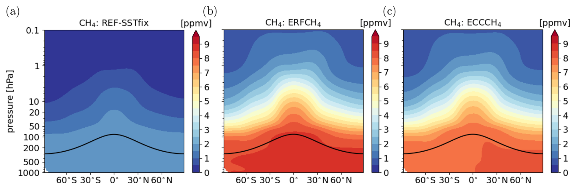
Figure 4 Annual zonal mean distribution of CH₄ mixing ratios in simulation (a) REF-SSTfix, (b) ERFCH₄ (fast response), and (c) ECCCH₄ (full response) in ppmv.

A similar effect was found by Winterstein et al. (2019), who analysed the fast response of 2 × and 5 × CH₄ surface mixing ratios in a set-up with prescribed CH₄ surface mixing ratios also using EMAC. The magnitude of the present CH₄ perturbation is comparable to their 5 × CH₄ experiment. In particular, to reach the prescribed CH₄ surface mixing ratios a pseudo surface emission flux is diagnosed in their set-up. The increase factor of the pseudo flux that corresponds to an increase of 5 × CH₄ is 2.75 (Stecher et al., 2021), exactly the increase factor of CH₄ surface emissions used in our study. Thus, in our study the increase of emission fluxes results in a close to 5-fold increase of the CH₄ surface mixing ratio. The global mean reference CH₄ mixing ratio and the corresponding pseudo emission flux are slightly lower in Winterstein et al. (2019), namely about 1.8 ppmv and 567.7 × 10¹² g CH₄ a⁻¹ (Tg (CH₄) a⁻¹). Additionally, the spatial distribution of their diagnosed pseudo flux is different and might be unrealistic. The latter two points explain why the increase factor of CH₄ mixing ratios is not exactly the same in our study. Nevertheless, the results suggest that the relation between the increase of CH₄ emissions and mixing ratios at the lower boundary is consistent if either the emissions or the mixing ratios are increased.

We derive the feedback factor f (see Eq. 1) from ERFCH₄ using two approaches. Firstly, it is calculated from Eq. (12) by Holmes (2018) as $f=\frac{\ln (m_{\mathrm{1}}/m_{\mathrm{0}})}{\ln (E_{\mathrm{1}}/E_{\mathrm{0}})}$. Secondly, it is derived from a curve fit of the function $m\left(t\right)=m_{\mathrm{0}}\times [{\mathrm{2.75}}^f+(\mathrm{2.75}-{\mathrm{2.75}}^f)\times \exp (-t/(f\times \mathit{\tau })\left)\right]$ (Holmes, 2018) of the spin-up of the atmospheric mass of CH₄ using the yearly mean CH₄ lifetime with respect to OH oxidation for τ (see Fig. S14). Both approaches suggest f = 1.55. However, the derived f is not expected to be representative of CH₄ perturbations of EMAC close to present-day conditions because f increases with increasing CH₄ burden (Holmes, 2018). This might also explain why our estimate of f is at the upper end of previous estimates (Fiore et al., 2009; Voulgarakis et al., 2013; Stevenson et al., 2013; Thornhill et al., 2021b; Stevenson et al., 2020; Sand et al., 2023).

In the stratosphere, CH₄ loss by OH is enhanced due to an increase of stratospheric HO_x, whereas CH₄ loss by Cl is reduced (see Table S1 in the Supplement). Overall, chemical stratospheric CH₄ loss is increased by 17.5 %. However, the increase of CH₄ mixing ratios is larger than the increase factor of surface emissions of 2.75 in the whole stratosphere as well.

In the full response, as shown in Fig. 4c, CH₄ mixing ratios are lower in comparison to the fast response, as shown in Fig. 4b. Similar to the climate response following the CO₂ perturbation, higher tropospheric temperatures lead to increased production of OH (see Fig. S3 in the Supplement). Additionally, the temperature-dependent reaction rate coefficient leads to a faster CH₄ oxidation. The corresponding sensitivity of the CH₄ lifetime per unit change in GSAT is −1.09 a K⁻¹ or −7.6 % K⁻¹ (relative to the lifetime in ERFCH₄). Both the absolute and the relative sensitivity are larger compared to the CO₂ perturbation experiment, which is possibly caused by the different CH₄ conditions in the respective fast responses (ERFCO₂ and ERFCH₄).

Stecher et al. (2021) analysed the climate response of the 2 × and 5 × CH₄ surface mixing ratio experiments corresponding to Winterstein et al. (2019). The sensitivity of CH₄ lifetime per unit change in GSAT corresponding to their 5 × CH₄ surface mixing ratio perturbation is $\frac{-\mathrm{1.17}\mathrm{a}}{\mathrm{1.28}\mathrm{K}}=-\mathrm{0.91}\mathrm{a}{\mathrm{K}}^{-\mathrm{1}}$, which corresponds to a relative change of −5.9 % K⁻¹ (relative to the lifetime in their fast response), and is thus less pronounced than the respective value of our study. The major difference between the simulation set-ups is that tropospheric CH₄ mixing ratios cannot respond to the lifetime response in the set-up of Stecher et al. (2021). This suggests that in the present study the sensitivity of CH₄ lifetime towards climate change is enhanced, because the CH₄–OH feedback is included in the response of OH and, therefore, in the CH₄ lifetime. The same is indicated by the results of the CO₂ perturbation as discussed above.

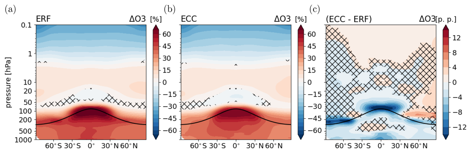
Figure 5 O₃ response following the CH₄ perturbation (same as Fig. 2 but for the CH₄ perturbation). Relative differences between the annual zonal mean O₃ mixing ratios of sensitivity simulations (a) ERFCH₄ (fast response) and (b) ECCCH₄ (full response) and their respective reference simulation in percent (%). (c) Climate response as the difference between the O₃ responses in panels (a) and (b) in percentage points (p.p.). Non-hatched areas are significant at the 95 % confidence level according to a Welch test based on annual mean values. The solid black line indicates the location of the climatological tropopause.

The response of O₃ is shown in Fig. 5. In the fast response (Fig. 5a), O₃ mixing ratios increase significantly throughout the troposphere, with a maximum increase of up to 60 % in the upper tropical troposphere. The CH₄ perturbation leads to enhanced O₃ formation by enhanced production of O₃ precursor species through CH₄ oxidation. In the stratosphere, radiatively induced cooling (a rapid adjustment) leads to O₃ increases in the middle stratosphere. Above 1 hPa, O₃ mixing ratios decrease due to enhanced catalytic depletion by odd hydrogen (HO_x). HO_x is increased by enhanced production of stratospheric H₂O caused by CH₄ oxidation (see Fig. S2 in the Supplement) and also by enhanced formation via the sink reaction of CH₄ with O(¹D). In the lower tropical stratosphere O₃ decreases, which can be explained by the reversed self-healing effect (Rosenfield et al., 2002; Portmann and Solomon, 2007), which is also effective for the CO₂ perturbation (see above). The fast response of O₃ is consistent with the fast response evolving in the comparable 5 × CH₄ surface mixing ratio experiment (Winterstein et al., 2019), as the same processes are effective, which are explained in more detail by Winterstein et al. (2019).

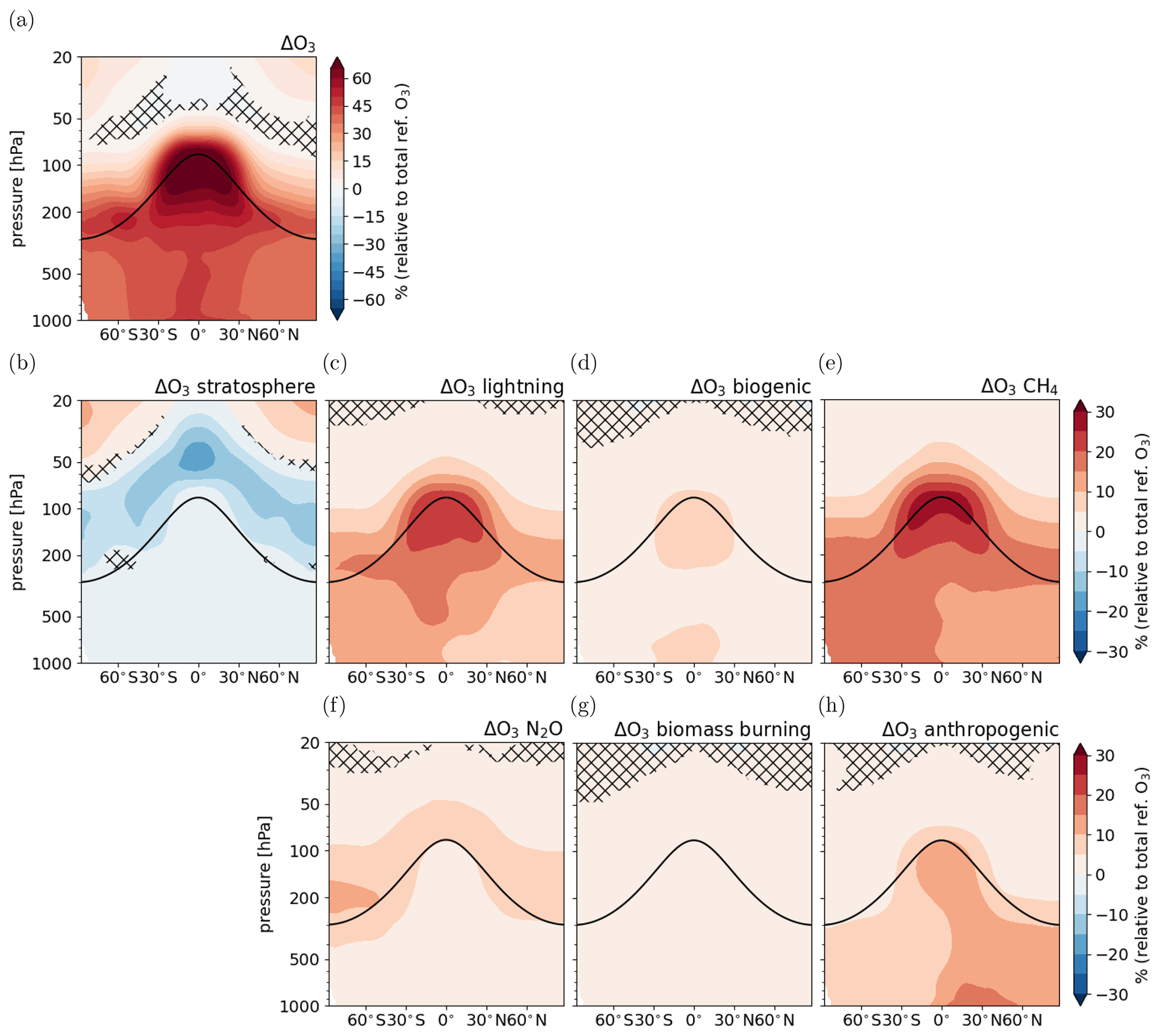
Figure 6 Fast response of tropospheric O₃ following the CH₄ perturbation: (a) response of total O₃ (same as Fig. 5a but data only shown up to 20 hPa to better compare with the response in the individual categories), (b–h) response of O₃ in individual source categories relative to total reference O₃ $\left(\mathrm{\Delta }{\mathrm{O}}_{{\mathrm{3}}_{\mathrm{cat}}}=\frac{{\mathrm{O}}_{{\mathrm{3}}_{\mathrm{cat},\mathrm{ERF}}}-{\mathrm{O}}_{{\mathrm{3}}_{\mathrm{cat},\mathrm{REF}}}}{{\mathrm{O}}_{{\mathrm{3}}_{\mathrm{total},\mathrm{REF}}}}\right)$. Non-hatched areas are significant at the 95 % confidence level according to a Welch test based on annual mean values. The solid black line indicates the location of the climatological tropopause.

Figure 6 shows the fast response of individual O₃ categories derived using the TAGGING submodel. Shown is the difference between ERFCH₄ and REF-SSTfix of one category relative to the total reference O₃:

$$\mathrm{\Delta }{\mathrm{O}}_{{\mathrm{3}}_{\mathrm{cat}}}={\displaystyle \frac{{\mathrm{O}}_{{\mathrm{3}}_{\mathrm{cat},\mathrm{ERF}}}-{\mathrm{O}}_{{\mathrm{3}}_{\mathrm{cat},\mathrm{REF}}}}{{\mathrm{O}}_{{\mathrm{3}}_{\mathrm{total},\mathrm{REF}}}}},$$

allowing a direct comparison with the relative response of total O₃. The O₃ mixing ratios increase in all categories except for the category O₃ stratosphere. This category shows reduced O₃ production through photolysis of O₂ in the lower stratosphere consistent with the reverse self-healing effect. The increase is strongest in the category O₃ CH₄, as the CH₄ increase directly leads to the formation of O₃. The increase in this category is most pronounced in the upper tropical troposphere and reaches up to 30 % relative to the total reference O₃. The larger abundance of NMHCs and CO also affects O₃ production of the other categories as their reaction with precursors from other categories, in particular NO_x, leads to enhanced O₃ production in the category O₃ CH₄ but also in the other categories. This effect is largest for the category O₃ lightning, which shows O₃ increases of up to 20 % relative to the total reference O₃, even though emissions of lightning NO_x decrease by 0.3 Tg (N) a⁻¹ globally in the ERFCH₄ simulation compared to REF-SSTfix (see Table 3). The CH₄ perturbation leads to upper tropospheric/lower stratospheric warming peaking at around 100 hPa in the tropics (see Fig. S1 in the Supplement). The higher static stability leads to less convection and thereby to decreasing lightning NO_x emissions. Upper troposphere/lower stratosphere warming following increased CH₄ has been already noted elsewhere and is expected to be even more pronounced if shortwave (SW) absorption by CH₄ is accounted for in the simulation set-up (Modak et al., 2018; Allen et al., 2023). Nevertheless, the enhanced abundance of precursors from CH₄ oxidation leads to enhanced O₃ production in this category. The category showing the third most pronounced increase is O₃ anthropogenic. Here, the increase of up to 15 % relative to the total reference O₃ is most pronounced in the lower NH, where the contribution of O₃ anthropogenic to total O₃ is largest.

The climate response of O₃ shown as the difference between full and fast response (see Fig. 5c) represents the isolated effect of the GSAT response on O₃. It shows a strong reduction of O₃ mixing ratios in the lower tropical stratosphere, which is caused by enhanced tropical upwelling (consistent with the CO₂ simulation). In the northern polar lower stratosphere, O₃ mixing ratios are enhanced, pointing towards strengthened poleward and downward transport (i.e. strengthening of the Brewer–Dobson circulation; see Fig. S13 in the Supplement) of stratospheric air masses. In the southern polar tropopause region the rise of the tropopause in the climate response leads to a large O₃ reduction. This process is also apparent in the NH, albeit less pronounced. Apart from that, the full response of O₃ in the stratosphere is mainly caused by the fast response. The climate response of tropospheric O₃ shows a reduction, except for the tropical middle troposphere, where the response shows a weak, not significant, increase in the zonal mean. In this region, enhanced emissions of lightning NO_x lead to enhanced O₃ formation (see also discussion of TAGGING results below). The climate response of O₃ is strikingly similar to the climate response pattern resulting from the CO₂ perturbation (see Fig. 2c), even though the fast response is different. The spatial distribution of the climate response of surface O₃ is likewise similar for the CO₂ and the CH₄ perturbation (see Fig. S4).

The similarity of the climate response patterns of O₃ resulting from CO₂ and CH₄ perturbations has been also noted by Stecher et al. (2021). However, the O₃ climate response resulting from their 5 × CH₄ mixing ratio increase shows a significant increase of O₃ in the tropical middle troposphere. As already stated, the main difference between their set-up and ours is that the feedback on CH₄ mixing ratios, and thereby also any secondary effects on O₃, is suppressed. As for the CO₂ perturbation, the reduction of CH₄ mixing ratios feeds back on O₃.

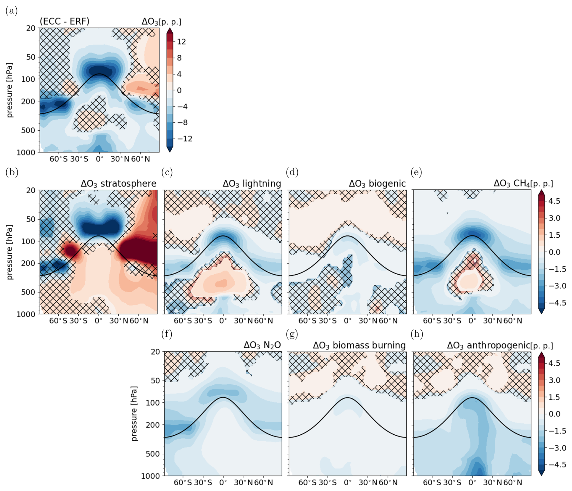
Figure 7 Climate response of tropospheric O₃ following the CH₄ perturbation (same as Fig. 3 but for the CH₄ perturbation): (a) response of total O₃ (same as Fig. 5c but data only shown up to 20 hPa to better compare with the response in the individual categories), (b–h) response of O₃ in individual source categories relative to total reference O₃ $\left(\mathrm{\Delta }{\mathrm{O}}_{{\mathrm{3}}_{\mathrm{cat},\mathrm{climateresponse}}}=\left(\frac{{\mathrm{O}}_{{\mathrm{3}}_{\mathrm{cat},\mathrm{ECC}}}-{\mathrm{O}}_{{\mathrm{3}}_{\mathrm{cat},\mathrm{REF}}}}{{\mathrm{O}}_{{\mathrm{3}}_{\mathrm{total},\mathrm{REF}}}}\right)-\left(\frac{{\mathrm{O}}_{{\mathrm{3}}_{\mathrm{cat},\mathrm{ERF}}}-{\mathrm{O}}_{{\mathrm{3}}_{\mathrm{cat},\mathrm{REF}}}}{{\mathrm{O}}_{{\mathrm{3}}_{\mathrm{total},\mathrm{REF}}}}\right)\right)$. Non-hatched areas are significant at the 95 % confidence level according to a Welch test based on annual mean values. The solid black line indicates the location of the climatological tropopause.

Figure 7 shows the climate response of individual O₃ source categories. It is calculated using Eq. (7) in accordance with the corresponding analysis of the CO₂ perturbation. The patterns of the climate response of the individual categories are overall consistent with those of the CO₂ perturbation.

The category O₃ stratosphere increases in the troposphere, indicating enhanced transport of stratospheric O₃ into the troposphere. The increase is significant everywhere, except for the extratropical SH and the lower tropical troposphere. This category contributes most strongly to the reduction of O₃ in the lower tropical stratosphere. The category O₃ lightning shows increases in the tropical middle troposphere resulting from an increase of the lightning NO_x emissions by 0.2 Tg (N) a⁻¹ in ECCCH₄ compared to ERFCH₄ (see Table 3) and decreases in the lower troposphere. Biogenic NO_x emissions increase by 0.37 Tg (N) a⁻¹ and biogenic C₅H₈ emissions increase by about 30 Tg (C) a⁻¹ as a reaction to climate change (see Table 3). However, the zonal mean climate response of O₃ in this category is mostly not significant and shows a decrease in the lower tropical and upper NH troposphere (see Fig. 7d). The tropospheric O₃ columns in this category increase locally over the Amazon region and the Congo River basin, where biogenic emissions of C₅H₈ increase the most, and the tropospheric O₃ columns decrease mostly over the tropical ocean (see Fig. S9 in the Supplement). As already mentioned, the sink of O₃ via the reaction of O(¹D) with H₂O is expected to strengthen in a warmer and moister troposphere. Similar to the CO₂ perturbation, the effects of increased O₃ precursor emissions and the enhanced chemical sink due to a larger abundance of tropospheric H₂O compete in this category. The category O₃ CH₄ decreases everywhere in the zonal mean, except for the tropical middle troposphere. The reduction is consistent with the reduction of CH₄ mixing ratios in the climate response, which leads to a reduced formation of O₃. In addition, the enhanced chemical sink leads to further reduction of O₃. The increase in the tropical middle troposphere coincides with the maximum increase of O₃ production from lightning NO_x emissions, which indicates that enhanced NO_x from lightning reacts with products of the CH₄ oxidation, resulting in an increased O₃ production in both categories. The corresponding response of the tropospheric O₃ columns is not significant in the tropics, because of the counteracting responses in the lower and middle troposphere, but shows a significant decrease in the extratropics (see Fig. S9 in the Supplement). The categories with prescribed O₃ precursor emissions, O₃ biomass burning and O₃ anthropogenic, show decreased O₃ mixing ratios throughout the troposphere (see Fig. 7g and h), consistently with the climate response resulting from the CO₂ perturbation. Additionally, reduced O₃ production per emitted molecule NO_x can play a role as O₃ precursor emissions of natural categories increase.

3.3 Radiative effects and climate sensitivity

Table 4 shows results for the total SARF, ERF, ΔGSAT, and the associated climate sensitivity parameters λ, as well as individual radiative effects corresponding to the composition changes in CH₄, O₃, and stratospheric H₂O. ERF includes physical and chemical adjustments, whereas SARF represents the radiative effect of the CO₂ or CH₄ composition change and the corresponding stratospheric temperature adjustment only.

Winterstein et al., 2019Stecher et al., 2021

Table 4 Estimates of total SARF, ERF, ΔGSAT, and the corresponding climate sensitivity parameters λ, as well as adjustments and feedbacks of individual composition changes in CH₄, O₃, and stratospheric H₂O. ERF includes physical and chemical adjustments, whereas SARF represents the radiative effect of the CO₂ or CH₄ composition change and the corresponding stratospheric temperature adjustment only. The climate sensitivity parameters λ_SARF and λ_ERF are calculated using SARF or ERF, respectively. Adjustments are calculated as the radiative flux changes in the fast response (in W m⁻²). Feedbacks are calculated as the difference of radiative flux changes between the full and the fast response divided by the corresponding change in global surface air temperature, ΔGSAT (in W m⁻² K⁻¹). The radiative effects of individual composition changes include the corresponding stratospheric temperature adjustment (Stuber et al., 2001). All radiative estimates are evaluated at TOA. In addition, the estimates of the 5 × CH₄ volume mixing ratio experiments analysed by Winterstein et al. (2019) and Stecher et al. (2021) are shown in the third column.​​​​​​​

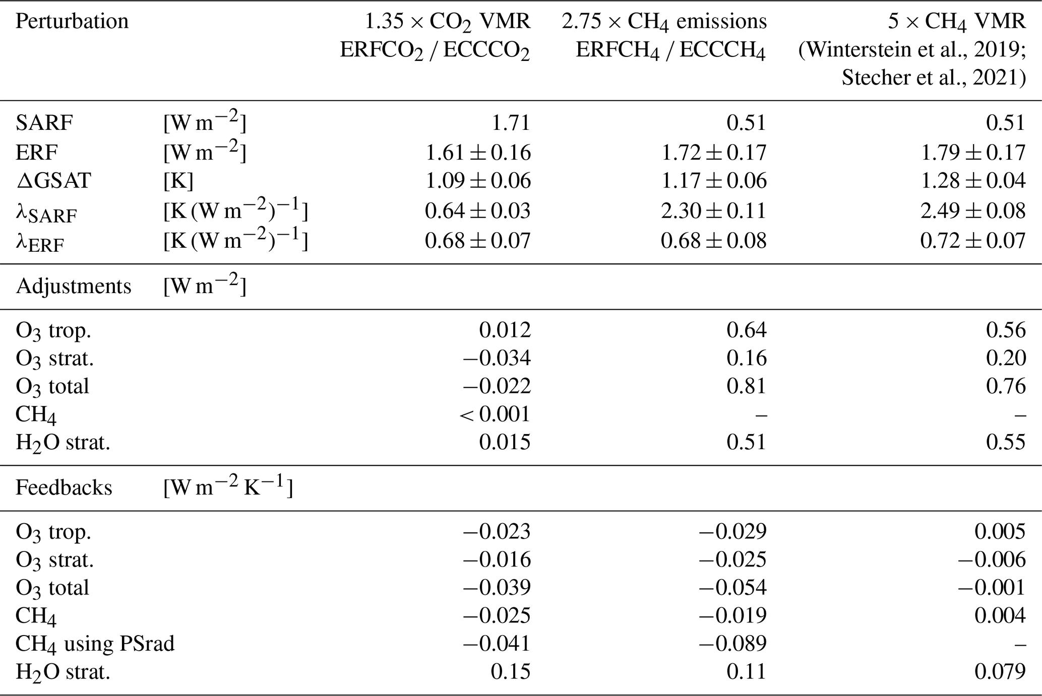
Values after the ± sign are 2 × the standard error of the mean calculated on the basis of 20 annual mean values, which approximate the corresponding 95 % confidence intervals. The standard errors for the climate sensitivity parameters are calculated from the standard error of the corresponding radiative forcing ​​​​​​​SE_RF and the standard error of ΔGSAT SE_ΔGSAT, as ${\mathrm{SE}}_{\mathit{\lambda }}=\left(\sqrt{\frac{{\mathrm{SE}}_{\mathrm{RF}}^{\mathrm{2}}}{{\mathrm{RF}}^{\mathrm{2}}}+\frac{{\mathrm{SE}}_{\mathrm{\Delta }\mathrm{GSAT}}^{\mathrm{2}}}{\mathrm{\Delta }{\mathrm{GSAT}}^{\mathrm{2}}}}\cdot \frac{\mathrm{\Delta }\mathrm{GSAT}}{\mathrm{RF}}\right)$.
The method to derive stratospheric-temperature-adjusted radiative estimates does not account for interannual variability, which is why no uncertainty estimates are provided for the respective estimates.

For the CO₂ perturbation, the estimate of ERF is smaller than SARF, but the difference is not significant due to the large statistical uncertainty associated with ERF (e.g, Forster et al., 2016). Along with this, the climate sensitivity parameter based on ERF, λ_ERF, is larger compared to λ_SARF, but the difference is not statistically significant either. In contrast, for the CH₄ perturbation, the estimate of ERF of 1.72 ± 0.17 W m⁻² is considerably larger than SARF, which is estimated at 0.51 W m⁻². The estimate of SARF reproduces the result of the comparable 5 × CH₄ mixing ratios experiment with the EMAC model (Winterstein et al., 2019). However, the radiative effect of CH₄ is known to be underestimated by the used radiative transfer scheme (Winterstein et al., 2019; Nützel et al., 2024). For instance, using the formula by Etminan et al. (2016)³ for the present CH₄ perturbation a SARF of about 1.7 W m⁻² is derived. The underestimation of the radiative effect of CH₄ affects the estimate of ERF as well. Under the assumption that all other adjustments remain the same, only the direct contribution of CH₄ is exchanged, which results in an ERF of about 2.9 W m⁻². This considerably larger ERF suggests a correspondingly larger response of GSAT as well.

As illustrated by Table 4, chemical adjustments play a minor role for the CO₂ perturbation. The fast response of stratospheric O₃ induces a negative adjustment of −0.034 W m⁻², whereas the fast response of tropospheric O₃ induces a positive adjustment of 0.012 W m⁻². The adjustment of tropospheric CH₄ is negligible, whereas stratospheric CH₄ induces a small positive adjustment due to its increase in the stratosphere and associated local radiative cooling. H₂O increases in the lowermost stratosphere by up to 5 % (see Fig. S2 in the Supplement), which leads to a positive adjustment of 0.015 W m⁻². The change in H₂O in the lowermost stratosphere is largely driven by a change in the tropical cold point temperature (CPT) (see Fig. S10). For the CO₂ perturbation, chemical production of H₂O in the stratosphere is slightly reduced up to about 2 hPa. Thus, the adjustment of stratospheric H₂O is unlikely to be chemically induced. To summarize, interactive chemistry dampens the ERF of the CO₂ perturbation by about −1.3 %, mainly by the effect of stratospheric O₃.

For the CH₄ perturbation, chemical adjustments of O₃ and stratospheric H₂O are important contributions to the ERF. The adjustment of tropospheric O₃ is 0.64 W m⁻², and that of stratospheric O₃ is 0.16 W m⁻². In addition, the adjustment of stratospheric H₂O is estimated at 0.51 W m⁻². The CH₄ perturbation leads to relative increases of H₂O up to 250 % in the upper stratosphere and mesosphere (see Fig. S2 in the Supplement) because the increased abundance of CH₄ leads to enhanced production of H₂O by CH₄ oxidation. Additionally, warming of the tropical cold point (see Fig. S10) leads to reduced dehydration of upwelling air parcels and thus to an increased abundance of H₂O in the lower stratosphere. The zonal mean warming of the tropical cold point is 1.5 K and thereby more pronounced than in the respective CO₂ experiment. The CH₄ perturbation induces a direct radiative heating at the tropical cold point of up to 1 K (see Fig. S12 in the Supplement), and the response of stratospheric O₃ leads to additional radiative heating of about 1.5 K in this region (see Fig. S12 in the Supplement). To summarize, the adjustments of O₃ and stratospheric H₂O enhance the ERF of the CH₄ perturbation by 1.31 W m⁻². The estimates of the adjustments of O₃ and stratospheric H₂O are consistent with the results of the comparable 5 × CH₄ mixing ratios experiment (Winterstein et al., 2019, see also column 3 in Table 4).

The feedback parameters represent the radiative effects induced by changes in composition related to the climate response, i.e. to the isolated effect of GSAT changes. They are, as usual, given in W m⁻² K⁻¹, i.e. normalized by the corresponding GSAT response. For both perturbation types, CO₂ and CH₄, the feedbacks of CH₄ and O₃ are negative, which means that they dampen the resulting temperature change. The feedback parameter corresponding to the CH₄ reduction in the CO₂ perturbation experiment is −0.025 W m⁻² K⁻¹. As already mentioned, it is known that the direct radiative effect of CH₄ is underestimated by the used radiative transfer scheme (Winterstein et al., 2019; Nützel et al., 2024). Therefore, we additionally calculate the feedback parameter for the same change in CH₄ mixing ratios, but with the PSrad radiation scheme (Pincus and Stevens, 2013; Nützel et al., 2024), using otherwise the same methodology (see Sect. 2.3). With PSrad, the CH₄ feedback is estimated at −0.041 W m⁻² K⁻¹, implying a more pronounced negative radiative feedback. Applying the formula of Etminan et al. (2016) for the change in CH₄ mixing ratio diagnosed from the simulation suggests a radiative effect of −0.059 W m⁻², which corresponds to a feedback parameter of −0.054 W m⁻² K⁻¹. Previous estimates of the CH₄ feedback have been derived offline from the change in atmospheric CH₄ lifetime and range from −0.014 ± 0.067 W m⁻² K⁻¹ (Thornhill et al., 2021a, if the estimates for changes in biogenic volatile organic compounds, lightning NO_x, and meteorology are combined⁴) over −0.03 ± 0.01 W m⁻² K⁻¹ (Heinze et al., 2019) to −0.036 W m⁻² K⁻¹ (Dietmüller et al., 2014). Our estimate using the PSrad scheme is at the upper end of previous estimates but in the range of estimates from individual models analysed by Thornhill et al. (2021a).

For the CH₄ perturbation, the feedback associated with the reduction of CH₄ mixing ratios in the full response in comparison to the fast response is −0.019 W m⁻² K⁻¹. Using the PSrad radiation scheme with otherwise the same method, the feedback parameter is estimated at −0.089 W m⁻² K⁻¹ suggesting a clearly larger influence. The radiative feedback of CH₄ corresponding to the 5 × CH₄ mixing ratio experiment (Winterstein et al., 2019; Stecher et al., 2021) does not include the reduction of CH₄ in the troposphere. The corresponding feedback parameter indicates a small positive feedback, caused by the larger mixing ratios of CH₄ in the stratosphere in the full response compared to the fast response (Stecher et al., 2021).

The feedback parameters corresponding to O₃ changes in the troposphere and stratosphere are both negative and add to total feedback parameters of −0.039 W m⁻² K⁻¹ for the CO₂ perturbation and −0.054 W m⁻² K⁻¹ for the CH₄ perturbation. Previous studies of the O₃ feedback resulting from CO₂ perturbations have assessed the full response in contrast to the climate response. The feedback parameter corresponding to the full response, i.e. including the adjustment, is −0.059 W m⁻² K⁻¹ in our study. Previous estimates range from −0.015 and −0.022 W m⁻² K⁻¹ (Dietmüller et al., 2014), −0.018 W m⁻² K⁻¹ (Marsh et al., 2016), −0.046 ± 0.018 W m⁻² K⁻¹ (Thornhill et al., 2021a), to −0.12 W m⁻² K⁻¹ (Nowack et al., 2015, if a corresponding GSAT response of 5.75 K is assumed). The feedback parameter of total O₃ in the present study lies in the range of previous estimates but, notably, is more pronounced than the estimate by Dietmüller et al. (2014), who also used the EMAC model. Part of the difference can be explained by the different sign of the feedback of tropospheric O₃. Dietmüller et al. (2014) found a positive feedback parameter of 0.008 to 0.009 W m⁻² K⁻¹ for tropospheric O₃ compared to the negative feedback parameter in this study. The reduction of tropospheric CH₄ mixing ratios leads to reduced O₃ production and thereby modifies the response of O₃ as discussed above. This indirect effect on O₃ is a consequence of applying emission fluxes instead of a prescribed lower boundary mixing ratio for CH₄. In addition, the negative feedback of stratospheric O₃ is also more pronounced in this study, which might be explained by the different magnitude of the perturbations. Dietmüller et al. (2014) noted differences between their 2 × and 4 × CO₂ experiments. Therefore, deviations for the 1.35 × CO₂ in this study can be expected. In addition, the different vertical resolution of the simulation set-ups might affect the response of stratospheric O₃. The results of the 5 × CH₄ mixing ratio experiment by Stecher et al. (2021) do not indicate a significant feedback of total O₃. This suggests that the reduction of CH₄ mixing ratios in the full response drives the negative O₃ feedback.

As explained above, the scaling factors of the CO₂ and CH₄ increase are chosen so that the resulting ERFs are comparable to allow an optimal comparison of the climate sensitivity of the two perturbation types, as the latter can depend on the magnitude of the radiative perturbation (e.g. Hansen et al., 2005; Dietmüller et al., 2014). The estimates of the climate sensitivity parameter based on ERF, λ_ERF, are identical for the CO₂ and CH₄ perturbations of this study. In contrast, the climate sensitivity parameters based on SARF, λ_SARF, differ significantly between the CH₄ and the CO₂ perturbation. This finding confirms the results of previous studies that the climate sensitivity is in general less dependent on the type of perturbation for ERF (e.g. Richardson et al., 2019). The use of λ_ERF as a climate sensitivity parameter to obtain an efficacy close to unity for the CH₄ perturbation is more important in this study compared to Richardson et al. (2019), because of the effect of interactive chemistry, which leads to larger differences between SARF and ERF for the CH₄ perturbation.

The estimate of λ_ERF of 0.68 ± 0.08 K (W m⁻²)⁻¹ is smaller than the corresponding estimate of the 5 × CH₄ mixing ratio experiment of 0.72 ± 0.07 K (W m⁻²)⁻¹ (Stecher et al., 2021). This suggests a reduction of the climate sensitivity parameter caused by the explicit simulation of the CH₄ reduction which would be physically consistent with the negative feedbacks of O₃ and CH₄ in this study. The difference between the two estimates is, however, not statistically significant.

4 Discussion and conclusions

In this study, we assess the feedback of atmospheric CH₄ resulting from changes in its chemical sink, which is mainly by oxidation with OH and which is influenced by temperature and the chemical composition of the atmosphere. We present results from numerical simulations with the CCM EMAC perturbed by either a 1.35 × CO₂ mixing ratio or a 2.75 × CH₄ emission flux increase. The scaling factors were chosen to reach a comparable ERF for both perturbation agents. EMAC is used in a CH₄-emission-flux-driven set-up, which allows the atmospheric CH₄ mixing ratio to adjust to changes in the chemical sink without constraints.

The increase of CH₄ emissions by a globally constant factor of 2.75 corresponds to an increase of the global mean CH₄ surface mixing ratio by a factor of 4.76. The larger increase of the CH₄ mixing ratio compared to the emissions is caused by a strong reduction of tropospheric OH, which leads to the extension of the tropospheric CH₄ lifetime. A similar effect was found by Winterstein et al. (2019), who analysed the response of 5 × CH₄ mixing ratios using a comparable set-up of the EMAC model, but with prescribed CH₄ surface mixing ratios. In particular, to reach the 5 × CH₄ mixing ratio increase, a pseudo surface emission flux is calculated in their set-up. The increase factor of the pseudo flux that corresponds to an increase of 5 × CH₄ is 2.75 (Stecher et al., 2021), exactly the scaling factor of CH₄ surface emissions used in this study. To summarize, reduced chemical decomposition enhances the increase of the CH₄ mixing ratios compared to the emissions. The relation between the increase of CH₄ mixing ratios and CH₄ emissions appears to be robust if either the mixing ratio or the emissions are increased.

We separately assess the so-called fast response in CO₂ and CH₄ perturbation simulations with prescribed SSTs and SICs, as well as the full response in simulations coupled to a MLO model. The CO₂ perturbation affects the chemical composition only indirectly through temperature changes. In the fast response, radiatively induced cooling in the stratosphere causes slower chemical depletion and therefore leads to increasing mixing ratios of O₃ and CH₄. In particular, our results show that the well-known increase of upper and middle stratospheric O₃ (e.g. Dietmüller et al., 2014; Nowack et al., 2015; Marsh et al., 2016; Chiodo et al., 2018) is part of the fast response and not related to the associated tropospheric warming. The CH₄ emission increase directly influences the chemical composition in the troposphere and stratosphere. The fast response patterns of O₃ and stratospheric water vapour are consistent with the changes following the 5 × CH₄ mixing ratio increase (Winterstein et al., 2019) as expected from the comparable magnitude of CH₄ mixing ratio increase.

Despite the different effect on the chemical composition in the fast response, the isolated effect of GSAT changes induced by either the CO₂ or the CH₄ increase is consistent. Tropospheric warming shortens the atmospheric lifetime of CH₄. The corresponding reduction of CH₄ mixing ratios is explicitly simulated by the used CH₄-emission-flux-driven set-up. The explicit reduction of CH₄ mixing ratios allows for secondary feedbacks on OH and O₃.

Firstly, the CH₄ lifetime response implicitly includes the CH₄–OH feedback. The sensitivities of the CH₄ lifetime per unit change in GSAT are −6.7 % K⁻¹ for 1.35 × CO₂ and −7.6 % K⁻¹ for 2.75 × CH₄, which is larger compared to previous CCM results using prescribed CH₄ mixing ratios at the lower boundary (Voulgarakis et al., 2013; Thornhill et al., 2021a; Stecher et al., 2021). The results of the comparable CH₄ increase experiment with prescribed CH₄ surface mixing ratios (Stecher et al., 2021) provide a clear indication that the lifetime change per temperature change is larger in the CH₄-emission-driven set-up. A comparable CO₂ increase simulation using EMAC with prescribed CH₄ surface mixing ratios is not available, but the comparison to the results of other CCMs (Voulgarakis et al., 2013; Thornhill et al., 2021a) indicates the same effect (see Sect. 3.1). Estimates of the CH₄ lifetime change per temperature change from other CCMs driven by prescribed CH₄ emission fluxes would be helpful to verify the influence of CH₄ emission fluxes in comparison to prescribing CH₄ at the lower boundary. Additionally, the multi-model differences of the CH₄ lifetime change per unit change in GSAT are large (Voulgarakis et al., 2013; Thornhill et al., 2021a), and it would be valuable to identify reasons behind CCM differences in future studies.

Secondly, the reduction of CH₄ mixing ratios results in reduced formation of O₃ in the troposphere. This leads to substantial differences in the climate response of tropospheric O₃ between this study and previous work using prescribed CH₄ mixing ratios at the lower boundary (Dietmüller et al., 2014; Nowack et al., 2015; Marsh et al., 2016; Nowack et al., 2018; Chiodo et al., 2018; Stecher et al., 2021). The latter studies consistently show an increase of O₃ mixing ratios in the tropical upper troposphere, whereas in this study the response is either insignificantly weak or indicates a reduction of O₃ mixing ratios in this region. An attribution method is used to identify and quantify the processes that influence tropospheric O₃ under climate change. Stronger stratosphere–troposphere exchange and larger natural emissions of O₃ precursors lead to increases of tropospheric O₃, whereas enhanced chemical loss caused by the increased tropospheric humidity and the reduction of CH₄ mixing ratios lead to decreases. The contribution of the individual processes depends on the representation of the process of the model. For instance, the representation of O₃ precursor emissions from natural sources is model dependent (e.g. Voulgarakis et al., 2013; Stevenson et al., 2020; Zanis et al., 2022). The climate response of lightning NO_x emissions is uncertain so that even the sign of the projected change depends on the used parameterization (Finney et al., 2016, 2018; Zanis et al., 2022). This has implications for the climate response of tropospheric O₃, for which changed lightning NO_x emissions are found to be an important contribution. Most schemes used in CCMs to date project increasing lightning NO_x emissions in response to tropospheric warming (Voulgarakis et al., 2013; Finney et al., 2016), which is in accordance with the results of this study, whereas a more sophisticated lightning NO_x parameterization indicates a decrease of lightning NO_x emissions (Finney et al., 2018). The spatial distribution of increases of biogenic C₅H₈ emissions over the Amazon region and the Congo River basin are in qualitative agreement with the climate response of biogenic emissions simulated by other CCMs (Zanis et al., 2022, see their Fig. S6). We expect the contribution of biogenic emission changes on O₃ to be more important than diagnosed by the used version of the TAGGING method, as it underestimates the influence of C₅H₈ emissions on the diagnostic tracer O₃ biogenic. The NMHC emissions are scaled by the number of C atoms in the molecule, i.e. five for C₅H₈, before they are added to the NMHC family tracer, which was not done in the case of the online calculated biogenic C₅H₈ emissions. We expect that this issue influences the quantitative response of the category O₃ from biogenic sources and more precisely that changes in O₃ biogenic caused by changes in C₅H₈ emissions are underestimated. However, we do not expect that the response patterns and general findings would change. Therefore, and due to the computational costs of the simulations, it was decided to not repeat the simulations. We also want to stress that this issue affects the diagnostic TAGGING results only but not the total O₃ response. Furthermore, biogenic emissions of C₅H₈ depend on the underlying vegetation, which is expected to interact with changes in, for example, climate, atmospheric CO₂ abundance, tropospheric O₃, or land use change (e.g. Zhou et al., 2018; Vella et al., 2023), but such interactions are not included in the used set-up. In addition, droughts can inhibit the substrate supply and thereby reduce biogenic C₅H₈ emissions (e.g. Wang et al., 2022). A respective representation of the impact of droughts on C₅H₈ emissions is not included in the used model version.

We calculate the radiative effects that correspond to the composition changes in CH₄, O₃, and stratospheric H₂O. Our results confirm that chemical adjustments of O₃ and stratospheric H₂O are important contributions to the ERF of the CH₄ perturbation. Therefore, ERF is significantly larger than SARF, which represents the direct radiative effect of CH₄ including the associated stratospheric temperature adjustment. The individual adjustments are in agreement with the estimates of the 5 × CH₄ mixing ratio experiment (Winterstein et al., 2019).

Chemical adjustments play a minor role in the CO₂ case. Here, stratospheric O₃ induces a negative adjustment, which reduces the ERF by about −1.3 %. Previous studies defined the full response of O₃ as its feedback (Dietmüller et al., 2014; Nowack et al., 2015; Marsh et al., 2016). Our results show that under the ERF framework a large part of the stratospheric O₃ change is to be regarded as an adjustment. Further, our results do not indicate that ERF is significantly different from SARF for the CO₂ perturbation, which is in accordance with simulation results, which account for physical adjustments only (Smith et al., 2018).

The scaling of the CO₂ and the CH₄ perturbations in this study is chosen so that the resulting ERFs are of similar magnitude. This allows an optimal comparison of the climate sensitivity parameters as these can depend on the magnitude of the perturbation (e.g. Hansen et al., 2005; Dietmüller et al., 2014). Our results suggest an efficacy of unity for the CH₄ perturbation when the climate sensitivity parameters are based on ERF. The climate sensitivity parameters based on SARF differ significantly between the CO₂ and the CH₄ increase, because of the large effect of chemical adjustments for the CH₄ perturbation. Thereby, our results support the finding that the climate sensitivity is in general less dependent on the type of perturbation for the ERF framework (e.g. Richardson et al., 2019). The multi-model mean efficacy based on ERF using the fixed SST method for a 3 × CH₄ perturbation analysed by Richardson et al. (2019) is slightly less than 1, with a spread of individual models of 0.56–1.15. In their study, the efficacy based on SARF is slightly less than 1 as well. In our study, the efficacy based on SARF is significantly larger than 1, i.e. about 3.6, because of the effect of chemical adjustments, which is not included in the estimate of Richardson et al. (2019).

The feedbacks corresponding to tropospheric O₃ changes in the full response are negative, in contrast to previous estimates derived with the EMAC model with prescribed CH₄ mixing ratios at the lower boundary (Dietmüller et al., 2014; Stecher et al., 2021). As mentioned above, the explicit reduction of CH₄ mixing ratios allows for secondary feedbacks on O₃ to evolve and leads, more precisely, to reduced O₃ formation, which is also reflected by the negative radiative feedback. Furthermore, the feedback parameter of tropospheric O₃ derived from the multi-model mean analysed by Stevenson et al. (2006) does not account for the CH₄ chemistry–climate feedback. The corresponding feedback parameter has been estimated at −0.007 ± 0.009 W m⁻² K⁻¹ by Heinze et al. (2019).

The reduction of CH₄ mixing ratios in the climate response induces a negative feedback parameter, which is estimated at −0.025 W m⁻² K⁻¹ for the CO₂ perturbation and at −0.019 W m⁻² K⁻¹ for the CH₄ perturbation using the default radiative transfer scheme of EMAC. However, it is known that this radiative transfer scheme underestimates the direct radiative effect of CH₄ (Winterstein et al., 2019; Nützel et al., 2024). Therefore, we derive the radiative feedback also with the PSrad radiation scheme (Pincus and Stevens, 2013; Nützel et al., 2024), which suggests clearly more pronounced feedback parameters of −0.041 W m⁻² K⁻¹ for the CO₂ perturbation and of −0.089 W m⁻² K⁻¹ for the CH₄ perturbation. The PSrad feedback parameters are in the range of previous individual model estimates derived from CH₄ lifetime changes (Dietmüller et al., 2014; Heinze et al., 2019; Thornhill et al., 2021a).

Further, the default radiation scheme used in EMAC so far does not account for absorption of CH₄ in the solar SW spectrum. Recent studies have shown that accounting for SW absorption by CH₄ influences adjustment and feedback processes of, for example, clouds (Smith et al., 2018; Modak et al., 2018; Allen et al., 2023, 2024). For an improved representation of the radiative effect of CH₄ in future studies, the PSrad radiation scheme (Pincus and Stevens, 2013) is now available for use in online EMAC simulations (Nützel et al., 2024).

This study focuses on the role of CH₄ for interactions between the gas-phase chemistry and climate change. However, further processes, which are not accounted for by the used simulation set-up, can also play a role. For instance, chemistry–aerosol–cloud coupling was identified to contribute to the ERF of CH₄ perturbations (Kurtén et al., 2011; O'Connor et al., 2022) and might therefore also influence the corresponding climate response. In addition, natural emission sources of CH₄, e.g. from wetlands or permafrost, have the potential to increase in a warming climate (e.g. O'Connor et al., 2010; Dean et al., 2018). For instance, the results of Thornhill et al. (2021a) suggest that the negative radiative effect corresponding to the shortening of the CH₄ lifetime is offset by the positive radiative effect of CH₄ emission increases from wetlands in response to a 4 × CO₂ perturbation. The net effect of feedbacks on the gas-phase chemistry and on natural emissions influences the effect of associated secondary feedbacks, e.g. regarding the formation of O₃.

To conclude, the atmospheric abundance CH₄, and therefore its potential as a greenhouse gas, is linked to a number of complex interactions. This makes the assessment of the climate feedback of CH₄ and its indirect effects a non-trivial undertaking, which requires comprehensive chemistry–climate simulations. The novelty of this study is that the feedback on CH₄ mixing ratios to changes in its chemical sink, and thereby also associated secondary feedbacks on OH and O₃, is accounted for explicitly, which is recommended to be adopted for further studies on chemical feedbacks.