Impacts of sea ice leads on sea salt aerosols and atmospheric chemistry in the Arctic

The processes contributing to Arctic cold-season (November–April) sea salt aerosols (SSAs) remain uncertain. Observations from coastal Alaska suggest that emissions from open leads in sea ice, which are not included in climate models, may play a dominant role. Their Arctic-wide significance has not yet been quantified. Here, we create an emission parameterization of SSAs from leads by combining satellite data of lead area (the Advanced Microwave Scanning Radiometer–Earth Observation System (AMSR-E) product) and a chemical transport model (GEOS-Chem) to quantify pan-Arctic SSA emissions from leads during the cold season from 2002 to 2008 and to predict their impacts on atmospheric chemistry, evaluating the results of our simulated SSAs against in situ observations. The AMSR-E product detects large leads with certainty (> 3 km in size), and, hence, our study is limited to quantifying emissions from large leads. Lead emissions vary seasonally and interannually. Simulated total monthly SSA emissions increase by 1.1 %–1.8 % (≥60° N latitude) and 5.6 %–7.5 % (≥75° N) for the 2002–2008 cold seasons. SSA concentrations primarily increase at the location of leads, where standard model concentrations are low. GEOS-Chem overestimates SSA concentrations at Arctic sites compared to ground observations, even when lead emissions are not included, suggesting underestimation of SSA sinks and/or uncertainties in SSA emissions from blowing snow and the open ocean. Multi-year monthly mean surface bromine atom (Br) concentrations increase by 2.8 %–8.8 % due to SSAs from leads for the 2002–2008 cold seasons. Changes in ozone concentrations are negligible. While leads contribute < 10 % to Arctic-wide SSA emissions in the years 2002–2008, these emissions occur in regions of low background aerosol concentrations. Leads may increase in frequency under future climate change, which could increase SSA emissions from leads.

1 Introduction

Sea salt aerosols (SSAs) affect Arctic climate by scattering incoming solar radiation and acting as cloud condensation nuclei and ice nuclei (DeMott et al., 2016; Pierce and Adams, 2006; Quinn et al., 1998). While, in the Arctic, there is no sunlight during polar night to scatter radiation, cloud condensation nuclei and ice nuclei can still have impacts on clouds and longwave radiation. Long-term measurements have shown that peak SSA concentrations in the Arctic occur during the cold season (Leaitch et al., 2018; Quinn et al., 2002; Schmale et al., 2021). However, the sources and mechanisms of cold-season SSA emissions are uncertain, which hinders atmospheric chemistry and climate models in accurately representing polar regions. Recent observations from Utqiaġvik, Alaska, have suggested that open leads – or open sea ice fractures – are an important source of cold-season SSA emissions (Kirpes et al., 2019; May et al., 2016). Climate change has impacted the Arctic by rapidly decreasing sea ice age and thickness (Intergovernmental Panel On Climate Change, 2023; Sumata et al., 2023; Vaughan et al., 2013), and future projections indicate that this will continue (Intergovernmental Panel On Climate Change, 2023), suggesting that the number of open leads will increase in the future due to thinner ice that is prone to fracturing. More work is needed to discern the Arctic-wide importance and impacts of SSA emissions from sea ice leads (“lead emissions”) with regard to atmospheric chemistry and climate. By combining satellite observations and chemical transport modeling, we quantify the significance and impacts of lead emissions in relation to atmospheric concentrations of SSAs and bromine and evaluate simulated SSAs against in situ observations.

While global models have not yet included SSA emissions from leads, several observational studies, largely based in Utqiaġvik, Alaska, suggest that emissions of SSAs from leads may be important. Key early observations made in the 1970s in Utqiaġvik by Scott and Levin (1972) and Radke et al. (1976) demonstrated an increase in sodium-containing particles in the presence of open-water leads. Since then, more recent measurement studies have quantified SSA emissions from leads. Nilsson et al. (2001) estimate that leads contribute an order of magnitude less than the open ocean to the Arctic SSA flux during the summer months. A multi-year study of observed SSAs at Utqiaġvik (May et al., 2016), conducted over all seasons, found that leads are a significant contributor to SSAs through wind-driven production, increasing the supermicron range in particular, but to a lesser extent than wind-driven production from the open ocean. Willis et al. (2018) suggest that lead emissions are more important in winter and early spring as winds over the northern oceans are at their highest. Kirpes et al. (2019) also convey the importance of seasonality, identifying SSAs produced by local leads as the dominant aerosol source in the coastal Alaskan Arctic during winter months. Chen et al. (2022), focusing on the spring in Utqiaġvik, show that leads were present locally throughout the study and contributed to sea spray aerosol production. As ground-based observations in the Arctic are mainly limited to coastal stations, such as Utqiaġvik, it is difficult to estimate the significance and impacts of lead emissions over the entire Arctic. Representing Arctic-wide emissions from leads in a global chemical transport model, especially during the cold season, will help discern whether lead emissions and their impacts on atmospheric chemistry are significant enough to warrant inclusion in chemistry and climate models.

Other modeling studies in the Arctic, along with observations, primarily from Antarctica, suggest that blowing snow is a potential major contributor of cold-season SSAs in polar regions. Blowing-snow SSAs come from saline snow over sea ice that is swept up by wind; the snow becomes salty through the upward movement of brine from sea ice to the snow surface, the incorporation of frost flowers, and the deposition of SSAs from the nearby open ocean (Domine et al., 2004). In two chemical transport models, the inclusion of additional SSA emissions from blowing snow brought simulated SSA mass concentrations closer to what was observed (Confer et al., 2023; Huang et al., 2018; Huang and Jaeglé, 2017; Rhodes et al., 2017). Other potential sources of cold-season SSAs, such as frost flowers, have been found to be insignificant (Alvarez-Aviles et al., 2008; Roscoe et al., 2011; Yang et al., 2017). Incorporating blowing-snow SSA emissions into models has shown how missing sources of SSAs in the Arctic can have a significant impact on atmospheric chemistry; for example, Huang et al. (2020) show that bromine released by blowing snow impacts modeled springtime bromine activation and ozone depletion events. The strong observational evidence regarding leads' contributions to cold-season SSAs and the impact of blowing-snow SSAs on modeled Arctic atmospheric chemistry suggests that there is a need to assess the potential impacts of lead emissions, which are currently missing from global chemistry and climate models. One study incorporated SSA emissions from leads in a chemical transport model (WRF-Chem), but the study was limited to the 400 km² area surrounding Utqiaġvik, Alaska, and used the ERA-5 reanalysis sea ice fraction to define the presence of leads (Ioannidis et al., 2023). Ioannidis et al. (2023) find that open leads are the primary source of fresh and aged SSAs in Utqiaġvik, Alaska, during the cold season, consistent with the observational analyses by May et al. (2016) and Kirpes et al. (2019).

SSAs play a critical role in Arctic tropospheric chemistry. SSA debromination is the main global source of reactive bromine in the troposphere (Wang et al., 2021). Reactive bromine chemistry has been attributed to the rapid depletion of ozone in the Arctic springtime, which reaches a maximum in March–April (Simpson et al., 2007). In particular, the bromine atom (Br) is key to these ozone depletion events; it is produced through the photolysis of Br₂, which is sourced from SSA debromination and snowpack chemistry (Abbatt et al., 2012; Dibb et al., 2010; Pratt et al., 2013; Stutz et al., 2011). Swanson et al. (2022) show improved springtime model–observation agreement with regard to BrO by including a snowpack photochemistry mechanism based on multiple field observations in a global chemical transport model. While, on a global scale, the reaction of OH with other SSA-sourced bromine species can also produce Br (Wang et al., 2021), this is minor in polar regions due to low OH concentrations. Br rapidly depletes ozone through heterogeneous reactions, producing BrO that can photolyze to reform Br, creating a catalytic ozone depletion cycle (Simpson et al., 2007).

Here, we estimate the pan-Arctic contribution of leads to total SSA emissions during the cold season for the years 2002–2008 by using satellite observations of lead area to parameterize lead-based SSA production in the global chemical transport model GEOS-Chem. We evaluate simulated SSA concentrations against observations and predict the impacts of lead SSA emissions on atmospheric chemistry, including concentrations of Br and ozone.

2 Methods

2.1 Satellite data of lead area fractions

In this study, we use satellite data of lead area fractions to inform the GEOS-Chem chemical transport model (next section) of where leads are present. The Advanced Microwave Scanning Radiometer–Earth Observation System (AMSR-E) sensor aboard NASA's Aqua satellite recorded brightness temperatures from Earth from 2002 to 2011 at six different frequencies (https://www.cen.uni-hamburg.de/en/icdc/data/cryosphere/lead-area-fraction-amsre.html, last access: 5 February 2025) (Integrated Climate Data Center (ICDC) et al., 2025), which are converted to lead area fractions following the algorithm of Röhrs and Kaleschke (2012). This method of detection can only be applied to the Arctic freezing season (November–April) due to surface melt of the sea ice modifying the sea ice emissivity from May to October, which affects the lead detection algorithm. Daily data are available at 6.25 km horizontal resolution as the algorithm is not limited by cloud cover. The AMSR-E satellite data are regridded to 0.5° × 0.625° from 6.25×6.25 km using a distance-weighted average remapping for consistency with the emission model's resolution (see Sect. 2.2 below for model details). For the rare individual days with missing data in the dataset (0.8 %), we use the average lead area fraction for that month. The lead area fraction includes open-water leads and thinly ice-covered leads 3 km and wider. The data span latitudes of 41° to 90° N, though a majority of Arctic sea ice lies above 60° N, with leads therefore being unlikely to be present at lower latitudes.

We use the AMSR-E lead area product for this study as it avoids cloud interference when detecting leads and provides a nearly consistent daily resolution. A limited quantitative validation by Röhrs and Kaleschke (2012) of the AMSR-E product against the Moderate Resolution Imaging Spectroradiometer (MODIS), conducted over of 1 d (21 March 2006), showed that 50 % of the total lead area visible in 500 m MODIS images was detected in the AMSR-E product. Leads greater than 3 km in size (“large leads”) were detected with certainty by the AMSR-E product (Röhrs and Kaleschke, 2012), and so our results effectively estimate emissions from large leads only.

2.2 GEOS-Chem: global chemical transport model

Here, we use the 3-D atmospheric transport model GEOS-Chem (geos-chem.org) version 13.2.1 (https://doi.org/10.5281/zenodo.5500717). Within GEOS-Chem, the Harmonized Emissions Component (HEMCO) computes emissions for different sources, regions, and species (Keller et al., 2014). GEOS-Chem and HEMCO are driven by Modern-Era Retrospective Analysis for Research and Applications, version 2 (MERRA-2) (Gelaro et al., 2017), meteorological fields from the NASA Global Modeling and Assimilation Office (GMAO), made up of reanalysis meteorological data assimilated from various observational sources (i.e., satellite, aircraft campaigns, and ground stations) providing variables such as temperature, wind, precipitation, and humidity. GEOS-Chem represents one-way interactions between the MERRA-2 meteorology and chemical constituents, meaning the meteorological conditions can affect the concentration of chemical species but not vice versa.

SSA emissions calculations for the open ocean use a wind- (Gong, 2003; Monahan et al., 1986) and sea-surface-temperature (SST)-dependent (Jaeglé et al., 2011) source function. In polar regions, SSA emissions from blowing snow are also included (Huang and Jaeglé, 2017). SSAs have two size bins: coarse mode (SALC; r=0.5 to 10 µm) and accumulation mode (SALA; r=0.1 to 0.5 µm). For gas and aerosol species, wet deposition (both rain and snow) includes washout and rainout in convective and large-scale stratiform precipitation (Amos et al., 2012; Liu et al., 2001; Wang et al., 2014). From November to April in the Arctic, wet deposition is mainly in the form of snow (Screen and Simmonds, 2012). Dry deposition of gas and aerosol species follows a resistance-in-series approach and includes gravitational settling of sea salt (Jaeglé et al., 2011; Pound et al., 2020; Wang et al., 1998; Zhang et al., 2001). Coupled gas- and multiphase-reactive halogen chemistry, including sea salt debromination, acid displacement, and photolysis and oxidation of gas-phase inorganic bromine and chlorine species, is described in Wang et al. (2021). This version of GEOS-Chem does not include snowpack chemistry as a source of reactive bromine in the standard model.

We parameterize SSA emissions from leads with the same function as the open-ocean emissions from Jaeglé et al. (2011) (Eq. S1 in the Supplement), scaled by the fractional area of leads in each grid cell from the AMSR-E satellite data. The Jaeglé et al. (2011) function is empirically derived to best match global observations in GEOS-Chem. We assume that leads emit SSAs at an equal rate as a function of lead area. This lead emissions parameterization is a unique wind- and SST-dependent source function for calculating lead emissions, driven by satellite observations defining the presence of leads. Figure 1 shows an example of the daily temporal frequency and spatial resolution of the AMSR-E satellite data (both the raw (a) and regridded (b)) used to drive the model.

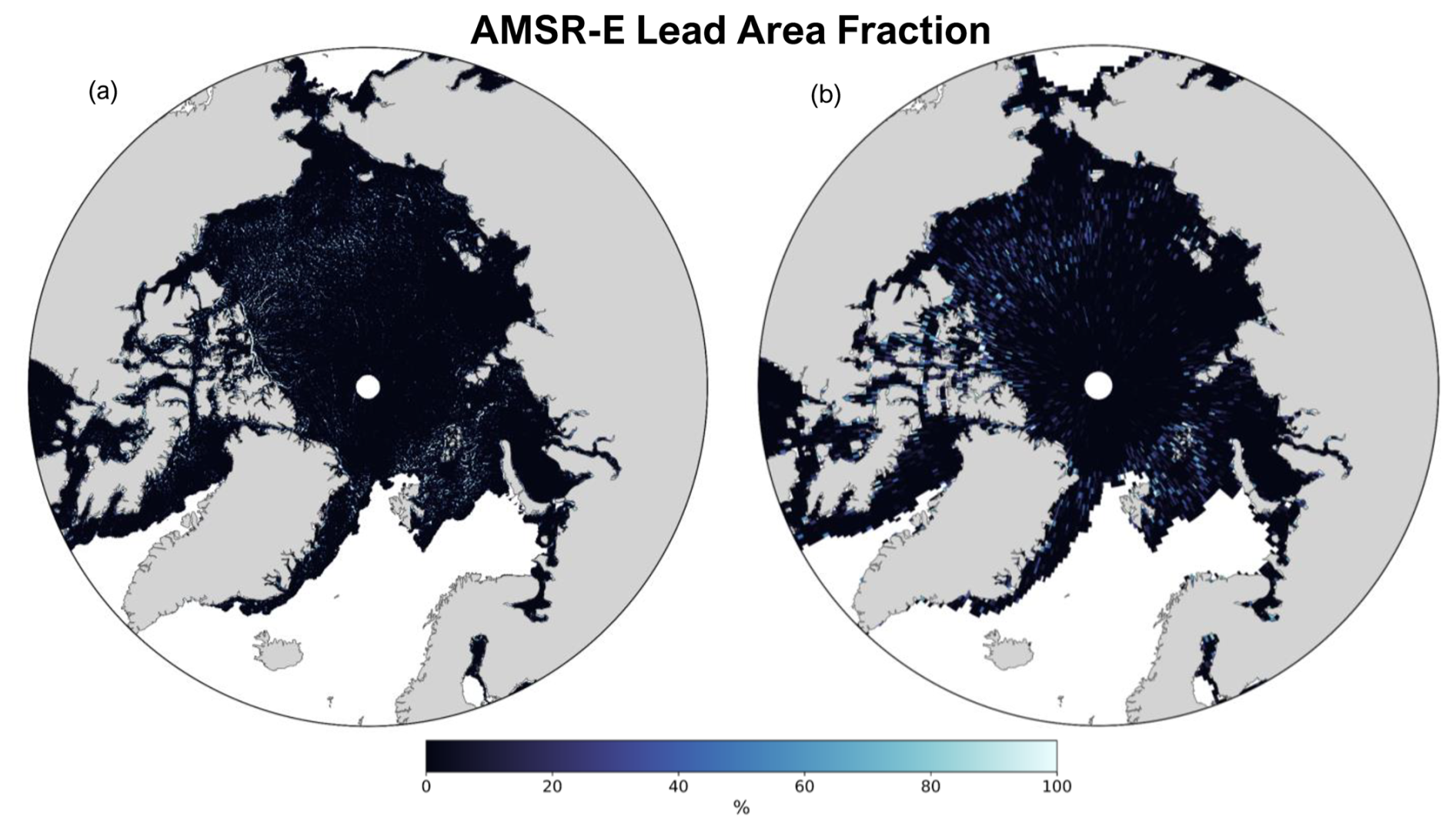
Figure 1 Map of AMSR-E daily lead area fraction in percent (%) for 1 November 2002: both raw (6.25 km resolution) (a) and re-gridded (0.5° × 0.625° resolution) (b).

We first calculate SSA emissions at the highest resolution of HEMCO (0.5° × 0.625°), which is the native resolution of MERRA-2. Two sets of emissions are calculated: (1) the standard emissions only (i.e., open-ocean and blowing-snow SSA emissions, the “standard” case) and (2) SSA emissions with lead emissions added (“standard + leads” case). Each set of emissions is then implemented separately into GEOS-Chem “offline” to ensure that total SSA emissions are properly scaled and distributed and not influenced by the resolution dependence of the wind speed (Lin et al., 2021). GEOS-Chem is run at the highest global horizontal (2° latitude × 2.5° longitude) and vertical (72 vertical levels) resolution. The absolute difference between the standard + leads and standard simulations is the change in SSA emissions or concentrations as a result of the leads, and we present the percent change due to leads (%) as calculated with Eq. (1).

$$\begin{array}{}\text{(1)}& \begin{array}{rl}& \mathrm{Percent}\mathrm{change}\mathrm{due}\mathrm{to}\mathrm{leads}\left(\mathit{\%}\right)=\mathrm{100}\times \\ & {\displaystyle \frac{(\mathrm{Standard}+\mathrm{leads}{)}_{\mathrm{simulation}}-(\mathrm{Standard}{)}_{\mathrm{simulation}}}{(\mathrm{Standard}{)}_{\mathrm{simulation}}}}\end{array}\end{array}$$

Simulations are performed for the years 2002–2008, when there is overlap between the AMSR-E satellite data and the available observed Arctic SSA concentrations at multiple sites, following 1 year of initialization. Because satellite observations of lead area fractions begin on 1 November 2002, we initialize the standard + leads case for GEOS-Chem with standard + leads SSA emissions for 1 year (1 November 2002 to 1 November 2003) and then start the simulation for analysis on 1 November 2002, with the spun-up 1 November 2003 initial conditions. For the standard case, the initialization year begins on 1 November 2001. For both cases, we simulate SSA concentrations, evaluate against observed concentrations, and assess the impacts of additional lead emissions on atmospheric chemistry. This includes an analysis of the change in the atmospheric concentrations of the bromine atom (Br) and ozone (O₃). For model evaluation, GEOS-Chem does not track sodium (Na⁺) content for SSAs, and so we convert simulated SSA into Na⁺ mass concentrations using a factor of $\frac{\mathrm{1}}{\mathrm{3.256}}$, which is based on the mass ratio of Na⁺ in seawater (Confer et al., 2023; Huang and Jaeglé, 2017; Riley and Chester, 1971).

2.3 In situ observations of Arctic sea salt aerosol concentrations

We evaluate simulated concentrations of SSAs from GEOS-Chem, converted into Na⁺ concentrations, against in situ observations of Na⁺ concentrations at four Arctic sampling sites: Utqiaġvik, Alaska (71.3° N, 156.6° W; 11 m a.s.l.) (Quinn et al., 2002); Zeppelin Mountain, Svalbard, Norway (78.9° N, 11.9° E; 475 m a.s.l.) (World Meteorological Organization (WMO), 2003); Alert, Nunavut, Canada (82.5° N, 62.5° W; 210 m a.s.l.) (World Meteorological Organization (WMO), 2003); and Pallas (Matorova), Helsinki, Finland (68° N, 24.24° E; 340 m a.s.l.) (Salmi, 2018). These observations are available for the time period of this study (November–April of 2002–2008, except for Pallas station, which covers 2003–2008). In winter months, the Utqiaġvik, Zeppelin, and Alert coastal sites border mostly ice-covered ocean (Huang and Jaeglé, 2017). At Utqiaġvik, mass concentrations of Na⁺ for submicron and supermicron aerosols are separated, while the other two sites measure the total mass concentration without a size distinction. The Na⁺ mass concentrations are determined from ion chromatography with uncertainties of 5 %–11 % or an absolute uncertainty of 0.01 µg m⁻³ (Quinn et al., 2000; World Meteorological Organization (WMO), 2003). The aerosol sampling frequency is daily at Zeppelin, Utqiaġvik (submicron), and Pallas and weekly at Alert and Utqiaġvik (supermicron).

3 Results

3.1 Emissions of sea salt aerosols from leads

Figure 2a shows the spatial distribution of multi-year (2002–2008) average lead emissions for the month of January, which is a climatology based on model simulations that use daily resolution lead data (e.g., Fig. 1). We focus Figs. 2 and 4 on the month of January as an example. January is tied for the highest lead emissions for latitudes of 60° N and greater and the second highest for latitudes of 75° N and greater (Table 1), and also has the second largest multi-year average lead area (see Fig. S3b in the Supplement). Alongside Fig. 2a is the standard model, which includes open-ocean and blowing-snow emissions (Fig. 2b; see Sect. 2.2). Total emissions are resolution independent and are shown in Fig. 2 for the 2.0° × 2.5° resolution of the online atmospheric chemistry simulation. We find that the lead emissions and lead area are spatially consistent (Figs. 1 and 2a) and occur in regions where the standard SSA emissions are low (e.g., in the Greenland Sea and parts of the Barents Sea). The percent change in SSA emissions due to leads (calculated with Eq. 1) is detailed in Table 1; Figs. 4, 5, and S4 show the percent change in SSA concentration due to leads. Generally, emissions tend to be higher from 70° to 80° N and more concentrated within the Bering Strait, the Nares Strait, Wynniatt Bay in the Canadian Archipelago, and the eastern Greenland Sea as opposed to off the coast of northern Russia and Europe. Month to month, regions where emissions are higher remain similar, while the magnitude varies (see Fig. S1).

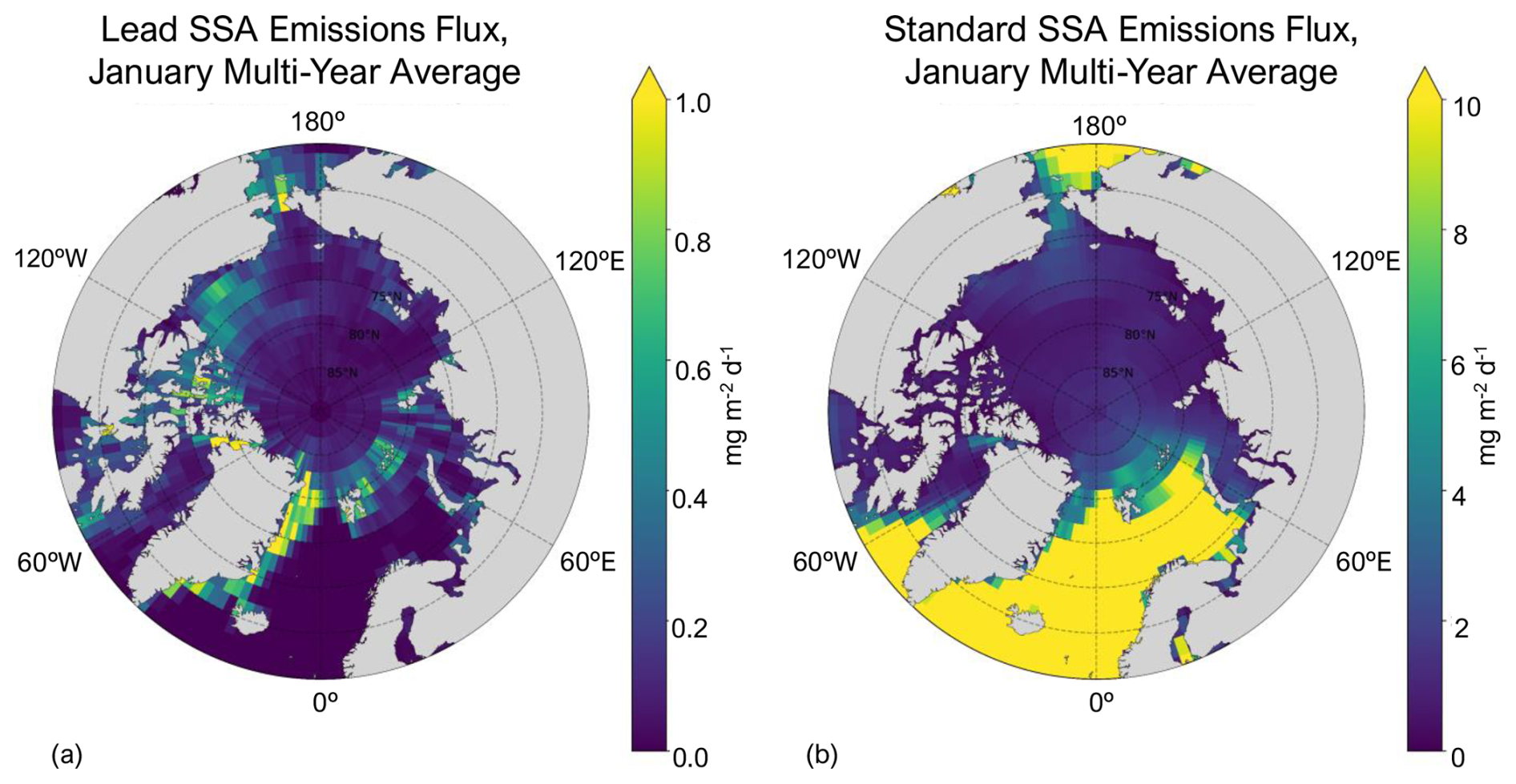
Figure 2 Total (coarse and accumulation mode) lead SSA emissions (a) and standard SSA emissions (b) averaged over 2002–2008 for January. Note the difference in magnitude in the color bar of (a) and (b).

Table 1 Multi-year (2002–2008) monthly average standard emissions and lead emissions ± 1 standard deviation (Gg) and percent change in SSA emissions due to leads ± 1 standard deviation in parentheses (calculated using Eq. 1), averaged for ≥ 60 and ≥ 75° N.

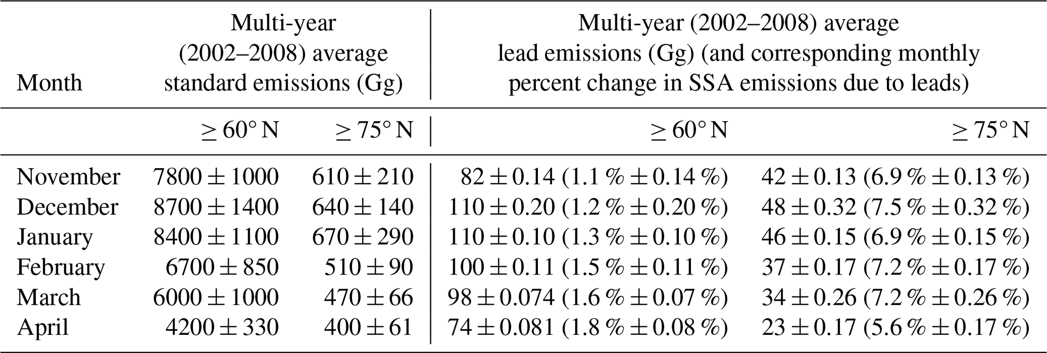
Table 1 shows the standard and lead emissions (in Gg), as well as the percent change in multi-year monthly average SSA emissions due to leads for 60° to 90° N latitude (≥ 60° N) and 75° to 90° N latitude (≥ 75° N). The standard deviations in Table 1 represent the year-to-year variability in emissions as the calculation is performed across the 7-year simulation time period for each month. Leads are relatively more important to total SSA emissions at higher latitudes due to large open-ocean emissions in the North Atlantic at lower latitudes (Table 1; Fig. 2b) and the spatial variability of the lead emissions (Fig. 2a). The month with the highest contribution to SSA emissions from leads varies with the region being analyzed. The smaller magnitudes of standard emissions later in the cold season poleward of 60° N make lead emissions relatively more important, with the largest percent increase ≥ 60° N in SSA emissions due to leads occurring in April. Poleward of 75° N, the lead emissions represent a larger fraction of the standard emissions, resulting in higher percent increases due to leads (∼ 4 %–6 % higher than for ≥ 60° N). In December, which is also the month with the highest percent increase due to leads ≥ 75° N, absolute lead emissions peak for ≥ 75° N latitude and decrease more than 2-fold by April. Controlling factors of the lead emissions are discussed in the next paragraph.

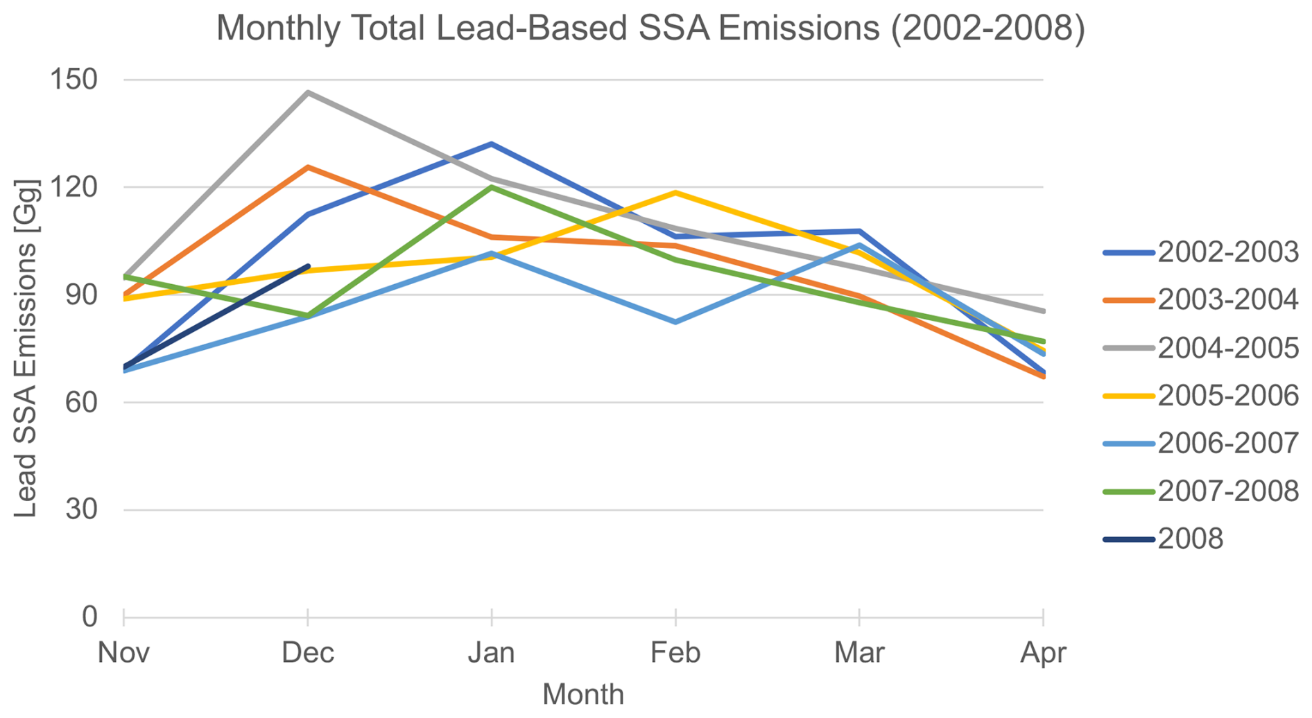
Figure 3 Monthly variations in total (coarse and accumulation mode) lead emissions of SSAs during the cold season for 2002–2008. Each line includes November and December of the first year and January through April of the following year, except for the year 2008, which only includes November and December of 2008.

We find that the magnitude of lead emissions varies by month and year, as well as seasonally (see Figs. 3, S1, and S2). Monthly total lead emissions and lead area have low correlation (R²=0.13; see Fig. S3), indicating that the variance in monthly total lead emissions is dominated by the nonlinear dependencies on wind speed and sea surface temperature (Eq. S1 in the Supplement) as the lead emissions are calculated with the Jaeglé et al. (2011) wind speed and sea surface temperature source function. In most years, lead emissions decrease from January to April, but there is no single month when lead emissions peak each year (Fig. 3). There is also no clear interannual trend in cold-season total lead emissions (see Fig. S2). Lead emissions are lowest in the 2006–2007 cold season and highest in the 2004–2005 cold season (Fig. S2). In the future, climate models predict that Arctic sea ice will continue to thin (high confidence) and that the presence of first-year vs. multi-year sea ice will increase (very high confidence) (Intergovernmental Panel On Climate Change, 2023), suggesting a possible future increasing trend in lead area and, therefore, lead emissions.

3.2 Atmospheric chemistry impacts of sea ice leads

Figure 4 shows the spatial distribution of the multi-year (2002–2008) average percent change due to leads in surface SSA mass concentration (a) and the absolute difference in SSA mass concentration between the standard + leads and standard simulations (b), as well as the standard simulated SSA mass concentration (c) for the month of January. With the addition of leads, the average Arctic-wide (≥ 60° N) percent increase in multi-year mean January SSA mass concentrations is 3.3 %, and the maximum percent increase in an individual model grid box is 60.5 %. We find that the greatest percent increases due to leads in SSA mass concentrations occur at the location of lead emissions (see Fig. 2a), where the standard concentrations are also very low, except off the eastern coast of Greenland, where the percent increase is reduced due to the high background SSA concentrations in the Greenland Sea (Fig. 4c) from open-ocean emissions (Fig. 2b).

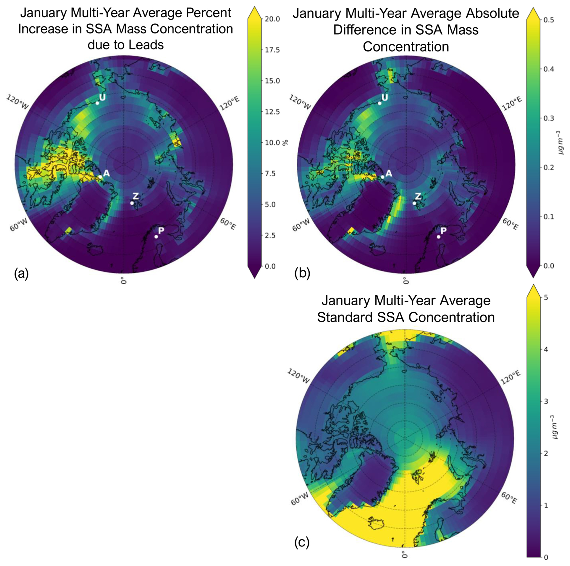
Figure 4 Percent change due to leads (calculated with Eq. 1) in SSA mass concentration (a), absolute difference between the standard + leads and standard SSA mass concentrations in µg m⁻³ (b), and the standard surface SSA mass concentration in µg m⁻³ (c) for the January multi-year (2002–2008) average. White points in (a) and (b) represent the locations of each observational site: Alert, Nunavut, Canada (A); Utqiaġvik, Alaska (U); Zeppelin Mountain, Svalbard, Norway (Z); and Pallas (Matorova), Helsinki, Finland (P). Note the difference in magnitude in the color bars for (b) and (c).

Figure 5a shows the average Arctic-wide percent increase, and Fig. 5c shows the absolute difference due to leads in the multi-year monthly mean SSA mass concentration for each cold-season month. Averaged poleward of 60° N, the percent increase and absolute difference due to leads in SSA mass concentration remain relatively constant throughout the cold season (Fig. 5a and c). Changes in monthly mean SSA mass concentrations are also higher poleward of 75° N. However, the percent increase in SSA mass concentration for both latitudinal ranges has large spatial variability, as seen in the standard deviation in Fig. 5a. The spatial distribution of the percent increase and absolute difference in SSA mass concentration due to leads remains similar month to month (see Figs. S4 and S5).

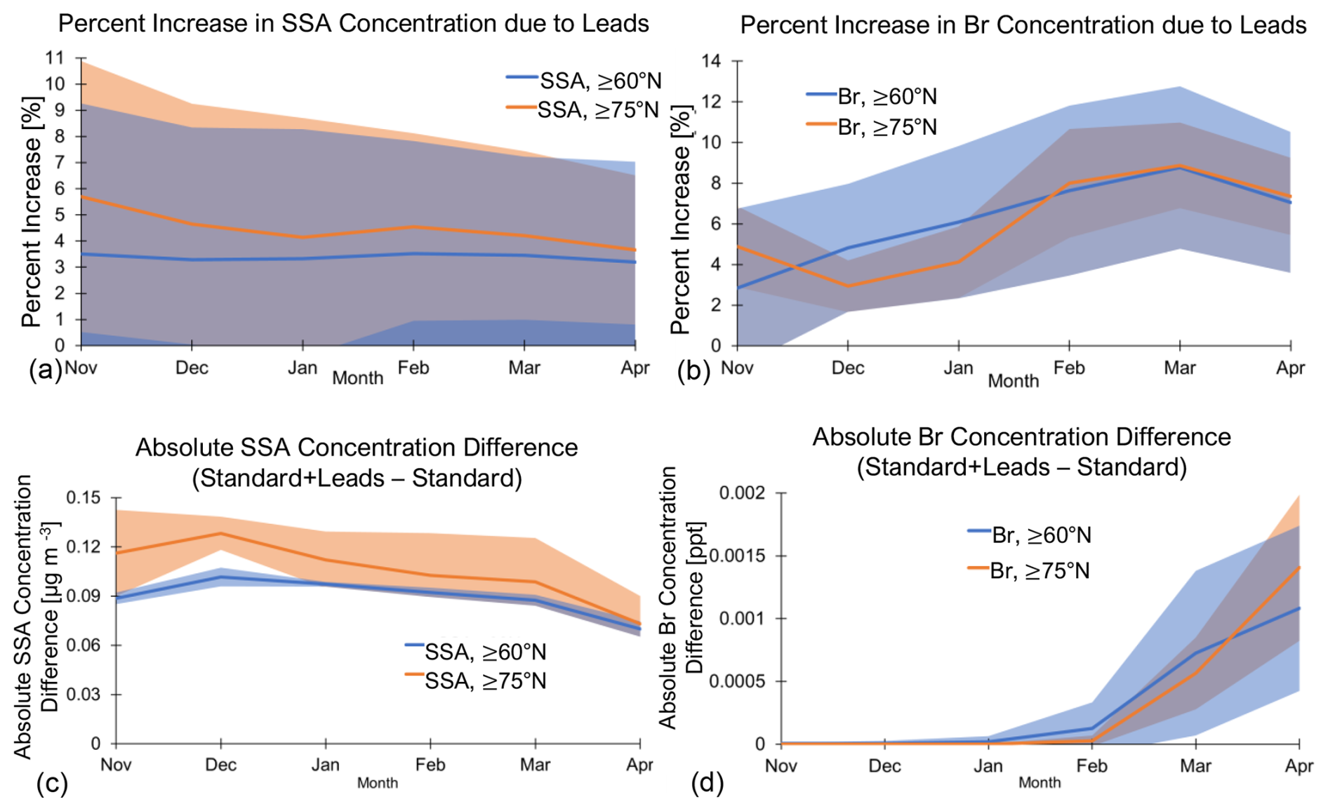
Figure 5 Multi-year (2002–2008) monthly mean percent increase due to leads (calculated with Eq. 1) in surface (a) SSA and (b) Br concentrations averaged across different Arctic regions (blue line: ≥ 60° N; orange line: ≥ 75° N). Shaded area represents ± 1 standard deviation.

As described in Sect. 1, SSAs contribute to the production of tropospheric reactive bromine and, thereby, the bromine atom (Br). Here, we examine changes in Br due to its role in ozone depletion events.

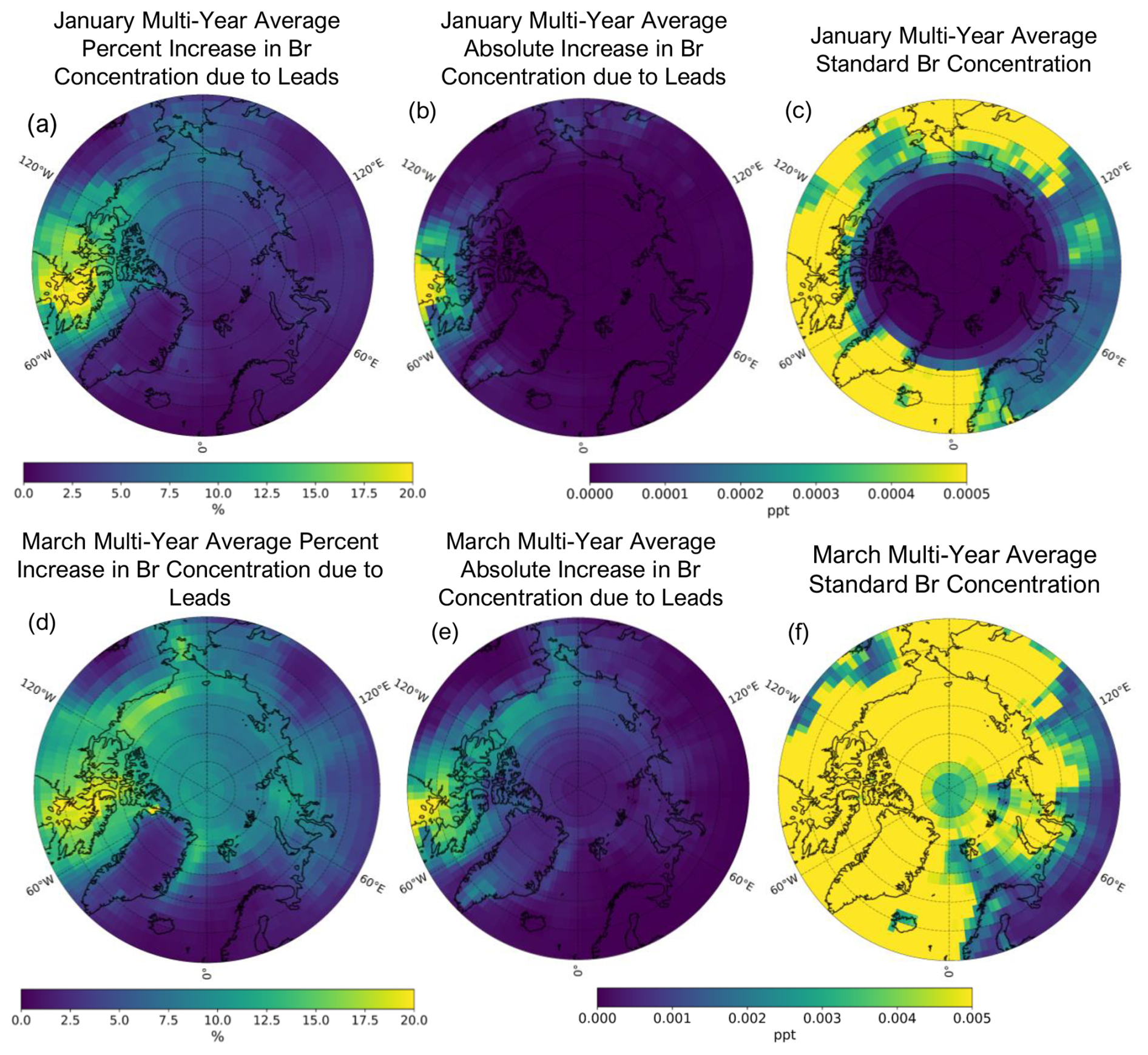
Figure 6 Multi-year (2002–2008) mean January (a, b, and c) and March (d, e, and f) percent increases due to leads in surface Br concentration (a and d), absolute increase in surface Br concentration due to leads (b and e), and standard model surface Br concentration in parts per trillion (ppt) (c and f). Note that the scales of the absolute difference and standard Br concentrations for the January and March multi-year averages show a difference of 1 order of magnitude.

Figure 6 shows the multi-year (2002–2008) mean percent increase and absolute difference due to leads in surface Br concentrations and the standard Br concentration (in parts per trillion or ppt) for the months of January (a–c) and March (d–f). Increased SSAs from leads increase surface levels of Br across all months during the cold season (Fig. 6a, b, d, and e; Figs. S6 and S7 for other months). These increased concentrations spatially follow the increased SSA mass concentrations from leads (Fig. 4a; Figs. S4 and S5 for other months), with differences due to where Br can be produced photochemically from the precursors released from SSAs. The spatial distribution of the percent increases in Br due to leads remains relatively similar month to month during the cold season (see Fig. S6) but with varying magnitudes (Fig. 6). The changes in Br concentration in February to April occur over a larger area (Figs. 6d and e, S6, and S7), likely due to the seasonality of Arctic bromine chemistry, which is influenced by the increasing area where sunlight is available to photolyze Br-sourced SSA species. The average Arctic-wide (≥ 60° N) percent increase due to leads in multi-year January mean surface Br concentrations is 6.1 %, and the maximum increase in an individual grid box is 35 %; for March, it is 8.8 % and 20.4 %, respectively. Overall, the average monthly percent increase in Br concentration is higher than the corresponding increase in SSA concentration, particularly after January, and reaches a maximum in March (see Fig. 5). The percent change due to leads in Br concentrations increases from November to March poleward of 60° N and from December to March poleward of 75° N (Fig. 5b). This does not strictly follow the seasonality of lead emissions (Fig. 3) or the percent increases in SSA concentrations due to leads (Fig. 5a), likely due to more available sunlight for photochemical reactions that produce Br later in the cold season. Increases in surface Br concentration could lead to decreased surface ozone concentrations. However, we find that the percent decreases due to leads in average surface ozone concentrations during the Arctic cold season are negligible ($<-\mathrm{0.25}$ %).

3.3 Evaluation against sea salt aerosol observations

We compare modeled and observed sodium (Na⁺) mass concentrations at four long-term monitoring stations to evaluate the performance of the simulations with and without additional lead emissions. The locations of each observational site are shown in Fig. 4a.

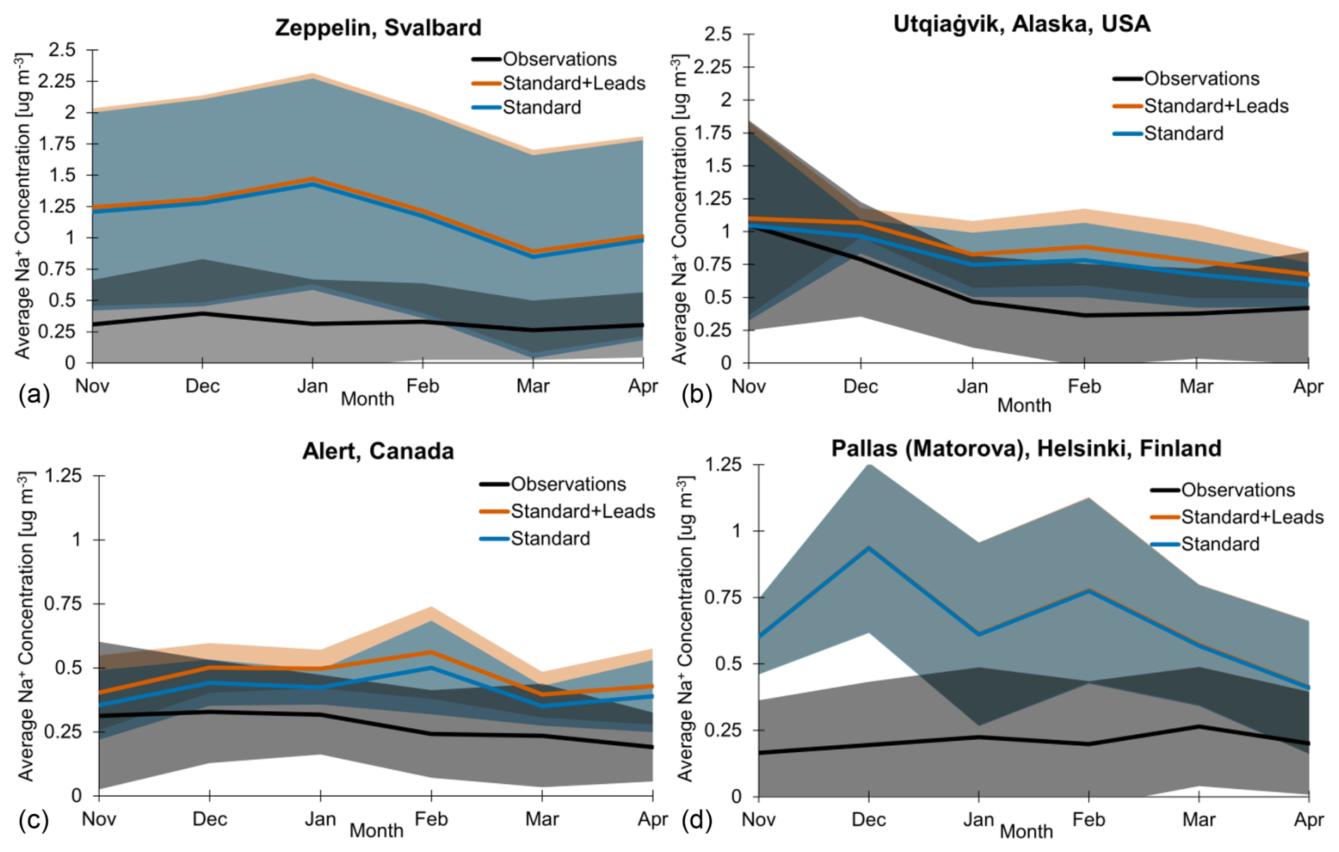
Figure 7 Observed (black line) and simulated (blue and orange lines) multi-year monthly mean sodium mass concentrations at (a) Zeppelin, Norway; (b) Utqiaġvik, Alaska; (c) Alert, Canada; and (d) Pallas (Matorova), Helsinki, Finland, for the cold seasons of 2002–2008 for (a)–(c) and the cold seasons of 2003–2008 for (d). Shaded regions are ± 1 standard deviation. Note that the y axes for Alert (c) and Pallas (d) are half as large as those for Zeppelin (a) and Utqiaġvik (b).

Figure 7 shows multi-year monthly mean Na⁺ concentrations in the observations (black), standard + leads simulation (orange), and standard simulation (blue) for Zeppelin (a), Utqiaġvik (b), Alert (c), and Pallas (d) during the cold seasons for 2002–2008 (a–c) and 2003–2008 (d). We sample the model simulations in the grid box that encompasses the latitude, longitude, and altitude of each monitoring station (see Sect. 2.3) and convert the simulated SSAs to Na⁺ concentrations. For all sites and months during the cold season, the simulated and observed Na⁺ mass concentrations overlap within ± 1 standard deviation (shaded regions in Fig. 7), except in November and December at Pallas. We find that the mean concentrations are overpredicted in both the standard and standard + leads simulations at all sites and in all months during the cold season, apart from the standard model at Utqiaġvik and Alert in November, with these agreeing most closely with the observations.

The model overpredicts Na⁺ concentrations the most at Zeppelin and Pallas, with the standard + leads and standard mean concentrations being a factor of 3.2 to 4.71 and 2.0 to 4.8 higher, respectively, than observations across all months during the cold season. Similarly, Confer et al. (2023) find an overprediction of SSAs at Zeppelin, which they find is exacerbated by including blowing-snow emissions. Additionally, Zeppelin is at a high elevation (located on a mountain at 475 m) and has been found to be more impacted by the free troposphere and aerosol–cloud interactions than other Arctic sites (Freud et al., 2017); the chemical transport model cannot represent two-way aerosol–cloud interactions. The model overestimate is less at Utqiaġvik, where the standard + leads simulation still overpredicts observed concentrations by a factor of 1.0 to 2.4, and least at Alert, with observed concentrations overestimated by a factor of 1.3 to 2.3 for the standard + leads model. Lead emissions do not change the simulated seasonality of cold-season surface SSA concentrations. The timing of cold-season maximum and minimum concentrations at Zeppelin, Alert, and Pallas differs between the observed and simulated cases (i.e., for both the standard + leads and standard models). At Utqiaġvik, the maximum mass concentration in the observations and both model simulations occurs in November. However, the minimum observed cold-season mass concentration occurs in February at Utqiaġvik, whereas the standard + leads and standard mean concentrations reach a minimum in April.

Figure 4a and b place the differences seen at each of the three sites in Fig. 7 into a broader context, with maps of the relative and absolute increases in SSA mass concentrations for the month of January. There is minimal change in SSA concentrations where Pallas is located, explaining the nearly equal Na⁺ concentrations for the standard + leads and standard simulations, which results in the overlapping lines in Fig. 7d, suggesting minimal influence from leads at this site, likely due to its inland location. The most significant relative increase in SSA concentration as a result of leads out of the four sites occurs at Alert (Fig. 7a). However, regions with the largest changes in SSA mass concentration due to leads, as in Fig. 4a and b, for the month of January (i.e., parts of northern Canada southwest of Alert), which are consistent throughout the cold season (Figs. S4 and S5) are not sampled by long-term ground monitoring sites, which would help constrain lead impacts on SSAs. In our simulation, lead emissions have the same size distribution as the open ocean, with most of the mass being found in the coarse mode (82 %–90 %). Despite this, there are increases in SSA concentration over land (Fig. 4a and b), indicating transport (see also Sect. S2 and Fig. S8). This is consistent with the observed inland transport of SSAs across the North Slope of Alaska (Simpson et al., 2005). It is likely that leads emit smaller SSA particles relative to open-ocean emissions (Nilsson et al., 2001), which would increase their lifetime; thus, non-local impacts from leads may be greater than simulated here. This further highlights the need for observations in other regions to better understand the impacts of lead emissions.

There is strong observational evidence that lead emissions contribute to cold-season SSAs (see Sect. 1), but the standard model consistently overpredicts observed SSA concentrations prior to the inclusion of additional lead emissions. This suggests that other sources of SSAs may be overpredicted or that sinks of SSA may be underpredicted. Ongoing work to improve the treatment of aerosol wet removal processes in GEOS-Chem has not specifically investigated the impacts on sea salt aerosols (Luo et al., 2020; Luo and Yu, 2023). Additionally, a recent observational study (Chen et al., 2022) suggests that the GEOS-Chem blowing-snow emissions parameterization may overpredict the frequency of blowing-snow events, therefore possibly contributing to the overprediction of Arctic SSA mass concentrations.

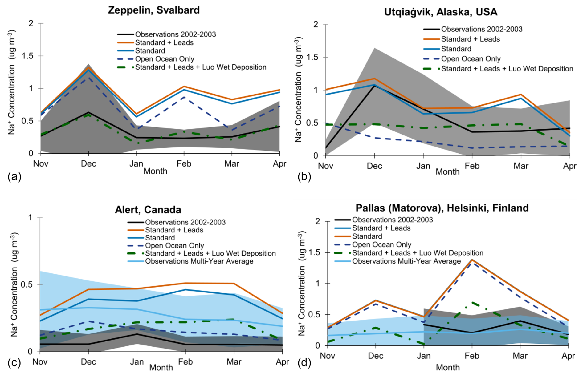
Figure 8 Model evaluation for the cold seasons of 2002–2003 at Zeppelin (a), Utqiaġvik (b), Alert (c), and Pallas (d). Observed Na⁺ concentrations are included as monthly averages for 2002–2003 (black, with standard deviation margin) and as the multi-year monthly averages (light blue, with standard deviation margin) (note that no 2002 data are available at Pallas). We show monthly average modeled Na+ concentrations for 2002–2003 for the standard + leads (orange) and standard (blue) simulations, with two additional sensitivity studies: open-ocean-only emissions contributing to Na+ concentrations (dark blue with dashes) and the standard + leads emissions with Luo et al. (2020) wet deposition applied (green line with dashes and dots). Note the different y axes for Alert (c) due to the fact that concentrations are much lower at this site.

To test these possible sources of uncertainty, we run two additional sensitivity simulations for one cold season (November 2002–April 2003): (1) using the Luo et al. (2020) wet deposition scheme with the standard + leads SSA emissions (“standard + leads + Luo wet deposition”) and (2) turning off blowing-snow emissions in the standard model for an open-ocean-only case (see Sect. S3 for further description). We find that the Luo wet deposition scheme improves model agreement most at Zeppelin (see Fig. 8a), especially in the months of November, December, March, and April. At Utqiaġvik, the Luo wet deposition scheme results in underestimates in Na⁺ concentrations compared to observations (Fig. 8b) in December, January, and April and overestimates in November, February, and March; however, the overestimated months are closer to the observed concentrations than the standard + leads and standard simulations. Additionally, the standard model at Utqiaġvik agrees with observations in December, and the standard + leads model agrees with observations in January and April.

At Alert, the Luo wet deposition scheme decreases the model overestimate of the standard + leads simulation when compared to the observations for the 2002–2003 cold season (Fig. 8c) but still overestimates Na⁺ concentrations in each month. As the 2002–2003 observations at Alert are particularly low, we also include the observed multi-year (2002–2008) monthly average Na⁺ concentrations for comparison. The Luo wet deposition scheme improves model evaluations from February to March compared to the multi-year average observed concentrations at Alert, but, otherwise, it underpredicts concentrations. The Luo wet deposition scheme decreases overprediction at Pallas in February compared to observations from the 2003 cold season, and it improves model agreement in March and April but underpredicts Na⁺ concentrations in January (Fig. 8d). As there are no available observations in 2002 at Pallas, we also include the observed multi-year (2003–2008) monthly average Na⁺ concentrations for comparison. The Luo wet deposition scheme underpredicts Na⁺ concentrations in November, January, and April and overpredicts concentrations in December and March compared to the multi-year average concentrations at Pallas.

At Utqiaġvik, underpredicted Na⁺ concentrations with only open-ocean emissions (except in November) suggest that this site is influenced by blowing-snow emissions and/or lead emissions. Of the four sites, blowing snow is the most important and the most well-represented here as it also improves the modeled seasonality by correctly representing the December peak in Na⁺ concentrations in the standard + leads and standard models; there may be larger uncertainty in the emissions parameterization in other regions. At Zeppelin, Alert, and Pallas, even with open-ocean emissions only and the standard wet deposition, the model overestimates Na⁺ concentrations for all months during the cold season for 2002–2003, except at Pallas in January, where only open-ocean emissions more closely match observations. Moreover, the open-ocean-only Na⁺ concentrations are close in value to the standard + leads and standard concentrations, indicating that Pallas is largely influenced by open-ocean emissions rather than by blowing-snow and lead emissions.

The results of these sensitivity tests suggest that changes to wet scavenging may be more important at higher altitudes, given the improvement in model evaluations at Zeppelin. Yet, the inclusion of the Luo wet deposition scheme in the standard + leads simulation still overestimates concentrations at Alert and generally leads to disagreement with observations at Utqiaġvik and Pallas (except in March and April at Pallas).

4 Uncertainty discussion

Our model evaluation reveals that SSAs are overestimated in the standard and standard + leads models at each of the four Arctic sampling sites, pointing to possible sources of uncertainty. First, we use the Jaeglé et al. (2011) open-ocean function for our lead emission parameterization as it is the standard SSA emission function in GEOS-Chem that has been previously evaluated across global oceans. However, there are possible differences in the mechanisms and meteorological dependencies of SSA emissions from leads vs. the open ocean, which could impact the magnitude and spatial patterns of lead emissions. Some potential differences were investigated in Nilsson et al. (2001), a summertime measurement study where an empirical lead emission flux equation with an exponential dependence on wind speed and with no consideration of SST was derived (Eq. S2). They found that the emissions rate per area from leads is smaller than that of the open ocean due to lower fetch in leads, which suggests that the lead emissions estimated in our study may be an upper limit when considering large leads only (> 3 km in size); however, this lead fraction detected by AMSR-E may only include 50 % of the total lead area (Röhrs and Kaleschke, 2012). Additionally, Nilsson et al. (2001) suggest that leads emit smaller SSA particles relative to the open ocean, which would increase their lifetime and transport distance. To create a more robust understanding of the different SSA emission mechanisms from leads vs. the open ocean, more studies using size-resolved observations could be conducted within the areas where we predict the highest lead emissions, such as within the Bering Strait, the Nares Strait, Wynniatt Bay in the Canadian Archipelago, and the eastern Greenland Sea.

Our sensitivity study results do not ultimately confirm the source(s) of overprediction within the GEOS-Chem model. Blowing-snow emissions are included as a standard source of SSA emissions in the Arctic, but remaining uncertainties about the GEOS-Chem blowing-snow emission parameterization (Chen et al., 2022) suggest a need for refinement. The results of the standard + leads + Luo wet deposition simulation highlight that there are also remaining uncertainties associated with wet deposition schemes as the Luo et al. (2020) mechanism does not lead to consistent improvement in simulated SSA concentrations. Luo and Yu (2023) find that the scheme overestimates wet scavenging on a global scale, and so continued improvement in the model deposition processes may resolve SSA overestimates. In addition, there are sparse ground observations of precipitation in the Arctic, and while the MERRA-2 reanalysis uses both model and satellite data to fill these gaps, Arctic cloud properties and precipitation can still be difficult to predict (Barrett et al., 2020; Taylor et al., 2019), which could affect the accurate simulation of aerosol deposition and, in turn, our simulated SSA concentrations.

5 Conclusions

Observational evidence (Chen et al., 2022; Kirpes et al., 2019; May et al., 2016; Radke et al., 1976; Scott and Levin, 1972; Willis et al., 2018) and one modeling study of the 400 km² region around Utqiaġvik, Alaska (Ioannidis et al., 2023), have shown that leads may be an important source of cold-season SSAs for the coastal Arctic. Here, we evaluate their importance as an Arctic-wide source of cold-season SSA emissions and their potential atmospheric chemistry impacts in the global chemical transport model GEOS-Chem.

We find that lead SSA emissions primarily occur in regions where other SSA emission sources are very low, mainly within the Bering Strait, the Nares Strait, Wynniatt Bay in the Canadian Archipelago, and the eastern Greenland Sea. Poleward of 75° N, leads increase total monthly cold-season SSA emissions by 5.6 % to 7.5 %, with the highest contribution of SSA emissions from leads in January and the lowest in April. Lead emissions vary in magnitude by month and year, mainly due to variations in lead area. Future trends in Arctic sea ice predicted by climate models suggest a possible future increasing trend in lead area (Intergovernmental Panel On Climate Change, 2023), which would increase lead emissions. The additional SSAs from leads in regions where the background aerosol concentrations are low could also affect local aerosol–cloud interactions, but the overall warming or cooling effect of these additional aerosols remains uncertain (Cox et al., 2015; Schmale et al., 2021; Stramler et al., 2011; Tan et al., 2023; Villanueva et al., 2022).

SSA mass concentrations primarily increase at the location of lead emissions in regions where the standard SSA mass concentration is very low (≤ 1.2 µg m⁻³). Throughout the cold season, the increased SSA mass concentrations from leads remain relatively constant in magnitude and spatial distribution. The highest increase in multi-year average SSA mass concentrations due to leads, spatially averaged for ≥ 75° N, occurs in November (5.7 % ± 5.2 %), and the lowest occurs in April (3.7 % ± 2.9 %). Increased SSAs from leads increase surface Br concentrations during the cold season in corresponding locations. We find that total Arctic-wide (≥ 60° N) increases in multi-year mean surface Br concentrations range from 2.8 % to 8.8 %. The increases in Br are not sufficient to have an impact on ozone; subsequent decreases in average surface ozone concentrations in the Arctic are negligible ($<-\mathrm{0.25}$ %).

Overall, we predict that sea ice leads may impact Arctic-wide cold-season SSA concentrations and Br concentrations by up to 5 %–10 %, on average, during the 2002–2008 period. As leads are likely to increase in prevalence under climate change, including this source of SSAs in chemistry and climate models may become more important for future predictions.