Technical note: A comparative study of chemistry schemes for volcanic sulfur dioxide in Lagrangian transport simulations – a case study of the 2019 Raikoke eruption

Lagrangian transport models are important tools to study the sources, spread, and lifetime of air pollutants. In order to simulate the transport of reactive atmospheric pollutants, the implementation of efficient chemistry and mixing schemes is necessary to properly represent the lifetime of chemical species. Based on a case study simulating the long-range transport of volcanic sulfur dioxide (SO₂) for the 2019 Raikoke eruption, this study compares two chemistry schemes implemented in the Massive-Parallel Trajectory Calculations (MPTRAC) Lagrangian transport model. The explicit scheme represents first-order and pseudo-first-order loss processes of SO₂ based on prescribed reaction rates and climatological oxidant fields, i.e., the hydroxyl radical in the gas phase and hydrogen peroxide in the aqueous phase. Furthermore, an implicit scheme with a reduced chemistry mechanism for volcanic SO₂ decomposition has been implemented, targeting the upper-troposphere–lower-stratosphere (UT–LS) region. Considering nonlinear effects of the volcanic SO₂ chemistry in the UT–LS region, we found that the implicit solution yields a better representation of the volcanic SO₂ lifetime, while the first-order explicit solution has better computational efficiency. By analyzing the dependence between the oxidants and SO₂ concentrations, correction formulas are derived to adjust the oxidant fields used in the explicit solution, leading to a good trade-off between computational efficiency and accuracy. We consider this work to be an important step forward to support future research on emission source reconstruction involving nonlinear chemical processes.

1 Introduction

Lagrangian transport models simulate the trajectories of air parcels that carry trace gases and aerosols through the atmosphere. These trajectories are determined using external datasets, which provide horizontal wind and vertical velocity fields obtained from meteorological reanalyses or forecast models. Lagrangian transport models are particularly useful for studying complex atmospheric processes, such as the interaction between different pollutants, chemical transformations, and the influence of different meteorological conditions. Lagrangian transport models have been widely applied in studies of natural and anthropogenic pollutant emissions. Applications of Lagrangian models include the simulation of point source or regional pollutant emissions, such as volcanic eruptions (Webster and Thomson, 2022), nuclear leakage accidents (Stohl et al., 2012), or wildfires (Evangeliou et al., 2019). They can also be used for global chemical transport simulations and source estimations of greenhouse gases such as carbon dioxide (CO₂) or methane (CH₄) (Bergamaschi et al., 2022; Che et al., 2022), long-lived gases of chlorofluorocarbons (CFCs) or hydrofluorocarbons (HFCs) (Pommrich et al., 2014; Brunner et al., 2017), fossil emissions (Dalsøren et al., 2018), and more. In contrast to grid-based Eulerian models, which represent fluid transport at fixed grid locations and suffer from numerical diffusion due to limited grid resolution, trajectory-based Lagrangian models generally have much lower numerical diffusion. In addition, Lagrangian models have the specific advantage of high scalability and computational efficiency, making them suitable for long-range and large-scale simulations. When simulating a large number of chemical species, Lagrangian models do not need to calculate transport separately for each species as in a grid-based Eulerian scheme (Brunner, 2012). However, Lagrangian models can face challenges such as complex boundary condition handling, difficulties in representing concentration fields and physical diffusion, high particle requirements for dense regions, and uneven computational loads.

In the past, Lagrangian models have often been used to qualitatively identify the source and reproduce the spatial distribution of plumes of trace gases, e.g., by tracking air parcels backward in time from receptors to sources to reconstruct the emissions (Wu et al., 2017; Pardini et al., 2017). In case studies of volcanic eruptions, the effects of SO₂ lifetime variations with altitude are usually neglected. However, Lagrangian models have the potential to be more quantitative. The essential step is to accurately model the physical and chemical processes for accurate prediction of the species' lifetime. For atmospheric species, such as SO_x, NO_x, hydrocarbons, and halocarbons, the chemical reactions have a significant impact on the estimation of their sources and sinks. Uncertainties introduced by chemical sinks can strongly influence the top-down source estimation (Stavrakou et al., 2013).

In the Lagrangian framework, the motion of species is simplified to time integration along trajectories determined by meteorological data. Species sinks are modeled separately for each air parcel, specifying the time derivative of the mass or mixing ratio of each species with an explicit rate. This method can represent processes such as dry/wet deposition, sedimentation, and first-order chemical reactions. For example, Liu et al. (2023) simulated the evolution of the SO₂ mass burden from the 2018 Ambae eruption with explicit loss rates, including wet deposition and gas-phase and aqueous-phase reactions, and they discussed the height sensitivity of SO₂ loss rates related to cloud distributions. For bimolecular or second-order reactions, where rates depend on the concentrations of two species, Liu et al. (2023) prescribed monthly zonal mean climatologies for OH and H₂O₂ to obtain pseudo-first-order approximations of the SO₂ oxidation. However, in dense volcanic SO₂ plumes, this approach may fail to capture oxidant depletion due to reactions with SO₂, particularly in regions of high SO₂ concentration. Accurate simulations under these conditions require dynamic coupling between reactant concentrations and reaction rates to properly represent second-order processes.

To model nonlinear chemical processes, an implicit chemical solver and an atmospheric mixing scheme should be considered (Brunner, 2012). In essence, while Lagrangian models efficiently track particle trajectories, a mixing scheme is essential to accurately represent diffusion and produce smooth gradients in concentration fields. Without a mixing scheme, particles carrying different reactants may remain isolated, resulting in pronounced local irregularities and inaccurate reaction rates. Mixing schemes address these issues by smoothing out irregularities in particle distributions, improving physical realism, and ensuring numerical stability. In recent years, three main types of Lagrangian chemical and mixing schemes have been considered. The first scheme uses a dynamically adaptive grid algorithm to mimic the stretching and distortion of air, such as in the Chemical Lagrangian Model of the Stratosphere (CLaMS) (McKenna et al., 2002b, a) and the Alfred Wegener InsTitute LAgrangian Chemistry/Transport System (ATLAS) (Wohltmann and Rex, 2009). The second scheme implements the chemistry scheme on a fixed 3-D grid, assuming uniform mixing of individual species within the grid boxes, such as in the UK Met Office's Next-Generation Atmospheric Dispersion Model (NAME) (Redington et al., 2009) and the Hybrid Single-Particle Lagrangian Integrated Trajectory (HYSPLIT) (Stein et al., 2000) model. The third scheme implements the chemistry scheme on the Lagrangian air parcels, but it uses a parameter to control the degree of mixing by adding a term to relax the trace gas concentrations in the air parcels to the background values averaged over a fixed 3-D grid, which is applied by the UK Meteorological Office (UKMO) chemistry transport model (STOCHEM) (Stevenson et al., 1998).

This paper focuses on the chemistry scheme implementation in the Massive Parallel Trajectory Calculations (MPTRAC) Lagrangian transport model (Hoffmann et al., 2016, 2022). Here, we selected the third approach outlined above, as it allows for online coupling of chemistry calculations with trajectory calculations, performed separately for each air parcel, followed by inter-parcel mixing, making it particularly suitable for large-scale parallelization. MPTRAC is designed for large-scale atmospheric simulations on high-performance computing (HPC) systems and has a hybrid message passing interface (MPI)–open multi-processing (OpenMP)–open accelerator (OpenACC) parallelization scheme implemented, demonstrating excellent performance and scalability on both CPUs (Liu et al., 2020) and GPUs (Hoffmann et al., 2024b). The model has been used in several case studies to simulate the long-range transport of volcanic SO₂, with emission estimates obtained from a backward-trajectory method (Wu et al., 2017, 2018; Cai et al., 2022) and a more complex and computationally intensive inverse modeling approach (Heng et al., 2016). In those studies, the height-dependent lifetime of SO₂ was not considered to be an influencing factor, as older versions of MPTRAC did not have a detailed chemistry scheme.

The main objective of this study is to introduce and assess a newly developed chemistry scheme with an implicit chemistry solver in the MPTRAC model that improves long-range chemistry transport simulations of volcanic SO₂ and allows for the estimation of volcanic emission sources. We propose a small chemical mechanism with 12 species and 31 reactions to model the production and loss of OH, HO₂, and H₂O₂ in the upper-troposphere–lower-stratosphere (UT–LS) region, including reactions among O(¹D), O(³P), H, OH, HO₂, O₃, and H₂O; reactions of SO₂ with OH in the gas phase; and oxidation with H₂O₂ in the aqueous phase. The aim is to model the dynamic OH and H₂O₂ fields as SO₂ oxidants to more realistically simulate and better represent the chemical lifetime of volcanic SO₂ in the UT–LS region. The chemical solver was built using the Kinetic Preprocessor (KPP) software package (Damian et al., 2002; Sandu and Sander, 2006). The KPP software provides a framework to automatically generate a Rosenbrock integrator for solving the stiff ordinary differential equations with specification of a chemical mechanism, including the chemical equations, species, and rate coefficients. The KPP has been widely used in atmospheric chemical modeling, for instance, in GEOS-Chem (Henze et al., 2007) and MECCA (Sander et al., 2019).

In a case study, we conducted simulations of the June 2019 Raikoke volcanic eruption to compare and verify the modeled lifetime of the SO₂ emissions with TROPOspheric Monitoring Instrument (TROPOMI) satellite measurements (Veefkind et al., 2012; Theys et al., 2017). The Raikoke (48.17° N, 152.15° E) eruption was a notable event that has been discussed in the literature to some larger extent. The eruption on 21–22 June was characterized by a series of explosive events that emitted SO₂ and volcanic ash into the lower stratosphere, impacting the stratospheric aerosol layer (Gorkavyi et al., 2021; Kloss et al., 2021). Cai et al. (2022) used MPTRAC to estimate the SO₂ emissions and investigate the effects of the injection height, time, and diffusion parameters on the simulation results. With an estimated 1.5 ± 0.2 Tg of SO₂, the eruption was notable for being the largest SO₂ injection into the upper troposphere and lower stratosphere since the 2011 Nabro eruption (Cai et al., 2022). In their publication, de Leeuw et al. (2021) discuss the transport and chemical evolution of SO₂ emissions resulting from the 2019 Raikoke eruption, offering a comprehensive comparison between NAME model simulations and TROPOMI observations.

This paper is organized as follows: in Sect. 2, we introduce the MPTRAC model, including the details of the implementation of the chemistry schemes, and the TROPOMI SO₂ satellite dataset; in Sect. 3, we discuss the results of the Lagrangian chemical transport simulations with MPTRAC for the Raikoke eruption, including the evaluation of the modeled SO₂ fields in the UT–LS region with the satellite data; and, finally, Sect. 4 provides the summary and conclusions of the study.

2 Data and methods

2.1 Overview on the MPTRAC model

Massive-Parallel Trajectory Calculations (MPTRAC) is a Lagrangian transport model that has been designed for heterogeneous CPU/GPU HPC systems and is particularly suitable for large-scale and long-term atmospheric simulations in the free troposphere and stratosphere (Hoffmann et al., 2016, 2022). The model requires meteorological input fields, in particular the horizontal wind and vertical velocity fields for the kinematic trajectory calculations, the temperature field for the chemistry calculations, and the cloud water fields for wet deposition and aqueous-phase chemistry. The trajectories of the air parcels are calculated using the explicit mid-point method to maintain the balance between computational efficiency and accuracy (Rößler et al., 2018). Following Stohl et al. (2005), diffusion is represented via stochastic perturbations added to the position of the air parcels, and subgrid-scale wind fluctuations are modeled as a Markov process using the Langevin equation. Unresolved convection is modeled via the extreme convection parametrization (Gerbig et al., 2003; Hoffmann et al., 2023). A comprehensive description of the model is given by Hoffmann et al. (2022). In the following section, we will discuss the two chemistry schemes implemented in the model in more detail.

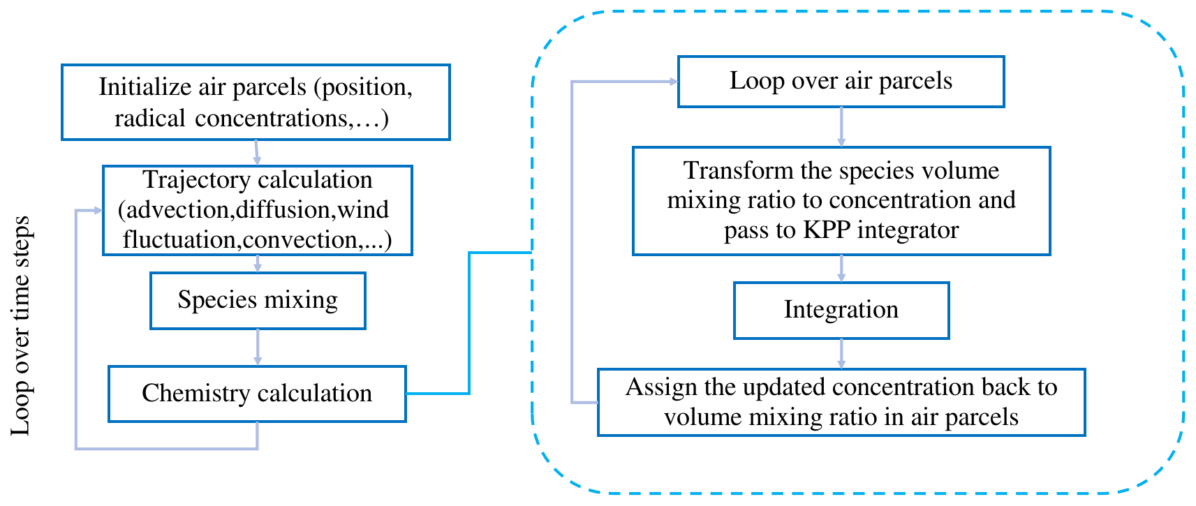
Figure 1 Simplified flow chart of the Massive-Parallel Trajectory Calculations (MPTRAC) Lagrangian chemistry transport model.

Lagrangian transport simulations with MPTRAC are driven by global meteorological reanalyses or forecasts. Here, we applied the fifth-generation reanalysis (ERA5; Hersbach et al., 2020) from the European Centre for Medium-Range Weather Forecasts (ECMWF); this reanalysis provides hourly meteorological data at a 0.3°×0.3° horizontal resolution on 137 vertical levels from the surface up to 0.01 hPa. Utilizing a state-of-the-art data assimilation system, ERA5 integrates a vast array of historical observations, including satellite and in situ data, to generate consistent, accurate, and temporally continuous records of meteorological information from the year 1950 to the present. The ERA5 data provide significant improvements with respect to meteorological information compared with the previous-generation ERA-Interim reanalysis (Dee et al., 2011), thereby benefiting the accuracy of Lagrangian transport simulations (Hoffmann et al., 2019).

2.2 Chemistry schemes and mixing in MPTRAC

2.2.1 First-order explicit chemistry scheme

In a Lagrangian model, linear decay processes over time t can be expressed as follows:

$$\begin{array}{}\text{(1)}& {\displaystyle \frac{\mathrm{d}y}{\mathrm{d}t}}=ky,\end{array}$$

where y represents the mass or volume mixing ratio (VMR) of a species in an air parcel. For a constant loss rate k, this ordinary differential equation is solved explicitly using the following exponential equation:

$$\begin{array}{}\text{(2)}& y(t+\mathrm{\Delta }t)=y\left(t\right)e^{-k\mathrm{\Delta }t}.\end{array}$$

Here, the rate coefficient k is prescribed as a model input. In MPTRAC, various loss processes such as wet/dry deposition or sedimentation are modeled in this way. When solving first-order chemical reactions, e.g., photolysis, the explicit solution has good computational efficiency, as it does not require numerical integration. The reactions of long-lived tracers with short-lived radicals can also be treated as pseudo-first-order reactions, assuming that production and loss of the radicals are in equilibrium and the pseudo-first-order rate constant k can be expressed as the product of the second-order rate coefficient k_2nd and the concentration of the oxidant [X], i.e., k=k_2nd[X].

In MPTRAC, prescribed radical species concentrations are taken from a monthly zonal mean climatology of Pommrich et al. (2014), which was prepared with the CLaMS model. In contrast to MPTRAC, which focuses on efficient particle transport with limited or simplified chemistry, the CLaMS model emphasizes detailed chemical reaction schemes for stratospheric processes. We consider the CLaMS model a reliable source for creating radical species climatologies for the UT–LS region. Following Liu et al. (2023), the OH field is scaled with a correction factor based on the solar zenith angle to mimic diurnal variations while preserving daily averages. Similarly, the monthly zonal mean H₂O₂ background field was obtained from the Copernicus Atmosphere Monitoring Service (CAMS) reanalysis (Inness et al., 2019) compiled into a monthly zonal mean climatology. At each time step, background field values are interpolated from the tabulated zonal mean data according to the pressure and latitude of the air parcels.

Regarding the SO₂ chemical reactions, the gas-phase oxidation with OH and the aqueous-phase oxidation with H₂O₂ are considered. In the cloud aqueous phase, H₂O₂ oxidation is the predominant pathway when pH < 5 (Seinfeld and Pandis, 2016; Rolph et al., 1992; Pattantyus et al., 2018). Other aqueous-phase oxidation pathways such as ozone oxidation and catalyzed oxidation via Fe(III) and Mn(II) are neglected because of low pH values in highly concentrated SO₂volcanic plumes. Liu et al. (2023) conducted a case study of the 2018 Ambae eruption with the first-order simplified chemistry scheme of MPTRAC, which provides more details.

2.2.2 Implicit chemistry scheme

Figure 1 shows a simplified flow chart of the MPTRAC model, including details of the chemistry calculations. The chemistry calculations follow the trajectory calculations and the mixing process. At each chemistry time step, the species' VMRs of each air parcel are multiplied by the molecular density of air to convert them into concentration units (molecules cm⁻³). After numerical integration of the chemical mechanism with the KPP integrator, the updated concentrations evolved in time are converted back to VMRs and assigned back to each air parcel. The chemical processes of different air parcels are calculated independently of each other, making this an ideal parallel-computing problem, which is particularly suitable for parallelization.

Our proposed chemistry mechanism for the decomposition of volcanic SO₂ in the UT–LS region includes 31 reactions and 12 species, as detailed in Table 1. This specific mechanism is newly proposed and has not been published or evaluated elsewhere. We developed the mechanism starting from SO₂ oxidation via OH in the gas phase (Reaction R31) and oxidation via H₂O₂ in the aqueous phase (Reaction R30), which are the major loss mechanisms for volcanic SO₂ (Rolph et al., 1992; Pattantyus et al., 2018; de Leeuw et al., 2021). Next, we integrated further reactions to model the dynamic production and loss of OH and H₂O₂.

Table 1 Proposed chemistry scheme for volcanic SO₂ oxidation in the UT–LS region.

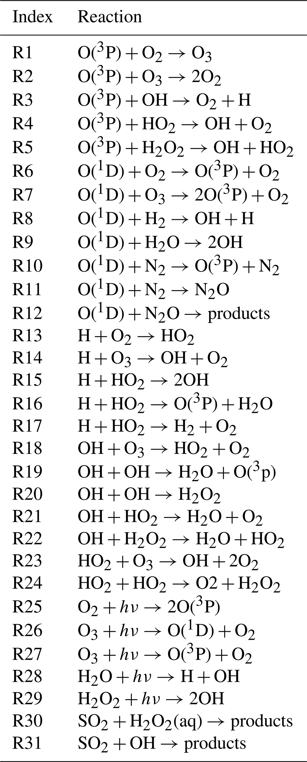
The production of OH mainly occurs via the reaction of H₂O with the excited oxygen radical O(¹D) (Reaction R9). The OH concentration exhibits a clear diurnal variation, due to a strong relationship with solar radiation (Reactions R25–R29), and a short lifetime resulting from self-reaction (Reactions R19 and R20) and reactions with O₃ (Reaction R18) and H₂O (Reaction R21) (Minschwaner et al., 2011; Tan et al., 2019). The H₂O₂ is primarily formed through the self-reaction of hydroperoxy radicals (HO₂) (Reaction R24), which are mainly produced via H and O₂ (Reaction R13) (Rieger et al., 2018). We incorporated additional reactions into the chemical mechanism, even though they are less relevant to the primary focus of volcanic SO₂ decomposition in the UT–LS, to capture potential secondary effects that might influence the system under certain conditions or improve applicability.

Note that this scheme for the oxidation of SO₂ was not designed for application in the boundary layer and lower troposphere, as it excludes nitrogen oxides, hydrocarbons, and carbon monoxide emissions and reactions. Furthermore, to simplify and constrain the chemistry calculations, each air parcel's ozone VMR is updated at every chemistry time step using ERA5 reanalysis data interpolation. Water vapor is also updated using ERA5 reanalysis data. The rate coefficients of all chemical reactions were taken from the current recommendations of Burkholder et al. (2019).

For photolysis modeling, we created 3-D photolysis rate look-up tables for the different species, $J=J({\mathit{\theta }}_{\mathrm{s}},\mathrm{TCO},p)$, where θ_s is the solar zenith angle, TCO is total column ozone, and p is pressure. The photolysis rate look-up tables cover 33 solar zenith angles from 0 to 96°, 8 total column ozone levels from 100 to 450 DU, and 66 pressure levels from 1013.25 to 0.1 hPa. The look-up tables were generated using the DISSOC photolysis module of CLaMS, originally based on Lary and Pyle (1991) and improved over time in several studies (Becker et al., 2000; Hoppe et al., 2014; Pommrich et al., 2014). Note that, for the DISSOC photochemistry model, we established the relationship between pressure, temperature, and ozone density via the U.S. Committee on Extension to the Standard Atmosphere (1976). The MPTRAC chemistry code determines θ_s, TCO, and p for each air parcel and linearly interpolates the corresponding J values from the look-up tables. The look-up table approach has the advantages of high computational efficiency and easy implementation on both GPUs and CPUs.

2.3 Wet deposition

Although the primary focus of this study is the comparison between the explicit and implicit chemistry schemes, it is also important to briefly outline the treatment of wet deposition in the MPTRAC model, as this is another significant loss process for volcanic SO₂ in cloud-containing environments. Wet deposition refers to the removal of SO₂ through processes such as precipitation scavenging, where SO₂ is dissolved in water droplets or ice crystals and subsequently removed from the atmosphere. Although the focus of this study is on chemical losses, it is crucial to consider wet deposition, particularly in tropical regions or during eruptions with high levels of atmospheric moisture, as it can significantly influence the lifetime of SO₂ and its transport in volcanic plumes. The interplay between wet deposition and chemical reactions in the presence of clouds contributes to the overall removal of SO₂ from the atmosphere, which is essential for accurate modeling of volcanic emissions and their impact on atmospheric chemistry.

In MPTRAC, wet deposition is implemented as a first-order loss term, where the removal rate of SO₂ depends on its concentration in the air parcel and the cloud water content. The in-cloud wet deposition rate is modeled via a rain-out process that considers the solubility of SO₂ and the precipitation rate, while the below-cloud deposition is represented by an empirical exponential formula based on precipitation intensity. This framework enables the model to account for the effects of cloud coverage and precipitation on SO₂ removal in both the gas and aqueous phase. The methodology for wet deposition in MPTRAC is detailed in Hoffmann et al. (2022) and has been modified and extended to address volcanic SO₂ deposition in Liu et al. (2023). Wet deposition has been considered in all simulations discussed in this paper.

2.4 Inter-parcel mixing algorithm

As mentioned in Sect. 1, atmospheric mixing is particularly important for properly modeling chemistry and transport in Lagrangian models (Brunner, 2012). The Lagrangian method inherently avoids numerical diffusion. A parameterization of mixing needs to be included to simulate transport and chemistry in a realistic manner. Here, we adapted the inter-parcel mixing scheme of Collins et al. (1997). This mixing scheme has the advantages of simple implementation and being well suited to CPU and GPU parallelization.

Following Collins et al. (1997), a relaxation term $d(c-\stackrel{\mathrm{‾}}{c})$ is added to bring the VMR value c of each air parcel closer to the average value $\stackrel{\mathrm{‾}}{c}$ within fixed grid boxes. A mixing parameter of d=0 means there is no mixing whereas a mixing parameter of d=1 means the species VMR is fully relaxed to the grid box mean. The parameter d therefore controls the degree of mixing. Default values of d are taken from Stevenson et al. (1998) to be 10⁻³ in the troposphere and 10⁻⁶ in the stratosphere. The grid box size was set to $\mathrm{5}\mathit{°}\times \mathrm{5}\mathit{°}\times \mathrm{1}$ km (longitude × latitude × log-pressure height). Mixing was conducted at every time step of the model, which is 180 s in this case.

2.5 TROPOMI SO₂ observations

In order to validate the simulated volcanic SO₂ distributions and lifetime for the Raikoke eruption, we used the Tropospheric Monitoring Instrument (TROPOMI) SO₂ Level 2 data product (Veefkind et al., 2012; Theys et al., 2017). TROPOMI is an ultraviolet, visible, near-infrared, and short-wavelength infrared spectrometer. It is mounted on the European Space Agency's Sentinel-5P satellite. The satellite operates in a near-polar Sun-synchronous orbit with an equatorial crossing time of 13:30 LT (local time) for the ascending nodes. TROPOMI samples the Earth's surface and atmosphere with a spatial resolution of 7×3.5 km² over a swath width of 2600 km. TROPOMI monitors ozone, methane, formaldehyde, aerosol, carbon monoxide, NO₂, and SO₂ in the atmosphere.

The TROPOMI Level 2 data include three SO₂ data products that provide SO₂ total column densities derived assuming a 1 km deep SO₂ layer centered at altitudes of 1, 7, and 15 km. In this study, we used the 15 km product because it best fits the SO₂ mass release from Raikoke volcano into the UT–LS region. To obtain the SO₂ total mass burden, we first averaged the TROPOMI retrieval data over horizontal grid boxes of 0.1°×0.1° and then integrated the averaged values of the grid boxes. Note that the TROPOMI SO₂ total column data are provided in Dobson units (hereafter denoted using DU). This is similar to ozone measurements; however, for SO₂, 1 DU corresponds to a total column density of $\mathrm{2.85}\times {\mathrm{10}}^{-\mathrm{5}}$ kg m⁻²​​​​​​​. A lower bound of 0.35 DU was applied to both the satellite measurements and the model results to reduce the effect of noise from the satellite measurements and to improve comparisons.

3 Results of the Raikoke case study

3.1 Model initialization and baseline simulation

In an earlier study, Cai et al. (2022) investigated the time- and height-resolved SO₂ injection parameters of the 2019 Raikoke eruption based on a backward-trajectory approach and SO₂ retrievals from TROPOMI observations. In this work, we used the same estimates of the SO₂ injections (as Cai et al., 2022) to initialize the release of air parcels in the transport simulations. A total SO₂ mass of 1.6 Tg was distributed over 10⁶ air parcels. The main injection peak occurs between 21 and 22 June 2019 at altitudes between 5 and 15 km. The vertical profile of the SO₂ injection rates is shown in Fig. 2. Numerical experiments were conducted with MPTRAC to compare the results of the linear-explicit and nonlinear-implicit chemistry solutions. Here, the simplified explicit approximation scheme is similar to the work of Liu et al. (2023), considering the gas-phase oxidation and aqueous-phase oxidation with climatological background OH and H₂O₂ fields (as introduced in Sect. 2.2.1). The KPP implicit solution considers the same reactions of SO₂, but the OH and H₂O₂ fields are modeled with the chemical mechanism listed in Table 1.

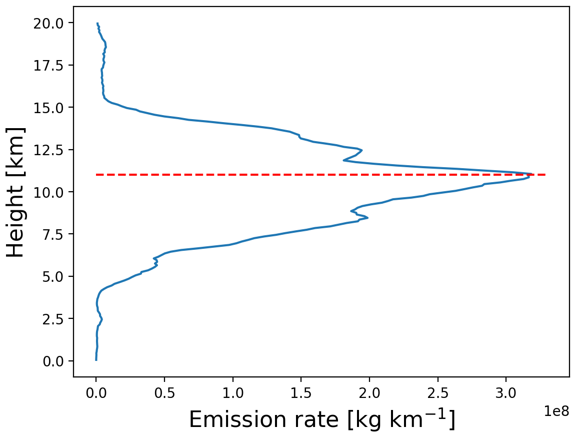
Figure 2 Vertical profile of SO₂ injections from the Raikoke eruption, as estimated by Cai et al. (2022). The red line represents the tropopause height at the location of the volcano.

The simulated SO₂ plume evolution with the KPP implicit chemistry scheme is compared with TROPOMI observations in Figs. 3 and 4. The explicit scheme closely matches the implicit scheme with respect to plume shape (not shown) but shows overall lower SO₂ column densities due to higher OH oxidation loss rates. Based on these comparisons, the MPTRAC model effectively captures the dispersion and transport of the volcanic SO₂ plume during the first 10 d after the eruption. Both the TROPOMI retrievals and the MPTRAC simulations show that the SO₂ plume continuously spreads over a larger area, with significant eastward motion and following the cyclonic flows. Consistent with the findings of Cai et al. (2022) and de Leeuw et al. (2021), the accuracy of the model results in reproducing the structural features of the observed SO₂ distributions gradually decreases after 15 d of simulation time due to error propagation. This decline is attributed to the limited resolution of the meteorological data, which also leads to a stronger diffusion effect. Nevertheless, the overall propagation direction and dispersion regions remain well aligned with observations. In this paper, we will focus on the analysis of the volcanic SO₂ mass evolution and chemical lifetime based on this baseline simulation.

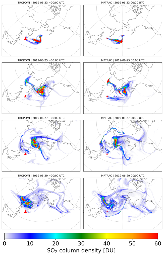
Figure 3 Evolution of SO₂ total column density distributions from 23 to 29 June 2019 from the MPTRAC simulation with the implicit chemistry scheme (right column) and the TROPOMI satellite observations (left column). The red triangle marks the location of the Raikoke volcano.

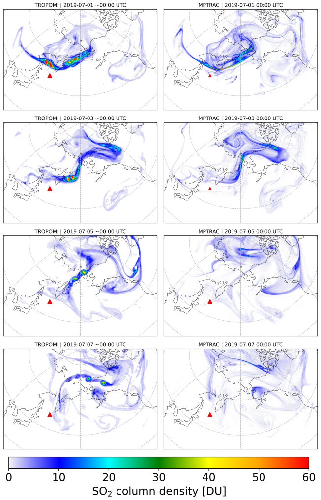
Figure 4 Same as Fig. 3 but from 1 to 7 July 2019.

3.2 SO₂ chemical lifetime analysis

The time evolution of the total SO₂ mass burden of the 2019 Raikoke eruption from the MPTRAC simulations and TROPOMI observations is shown in Fig. 5a. The total mass burdens from the model and the observations were obtained by integrating the SO₂ column densities on a 0.1°×0.1° horizontal grid. For this comparison, the satellite data and the grid output of the model were sampled with a lower detection limit of 0.35 DU and weighted by the mean kernel function of the TROPOMI observations to reduce the impact of noise and other uncertainties and to account for the vertical sensitivity of the measurements. It is found that the SO₂ lifetime modeled with the implicit KPP solution is about 1.6 times larger than that of the simplified explicit approximation. This can also be seen from a comparison of the vertical profiles of the e-folding lifetimes in Fig. 6.

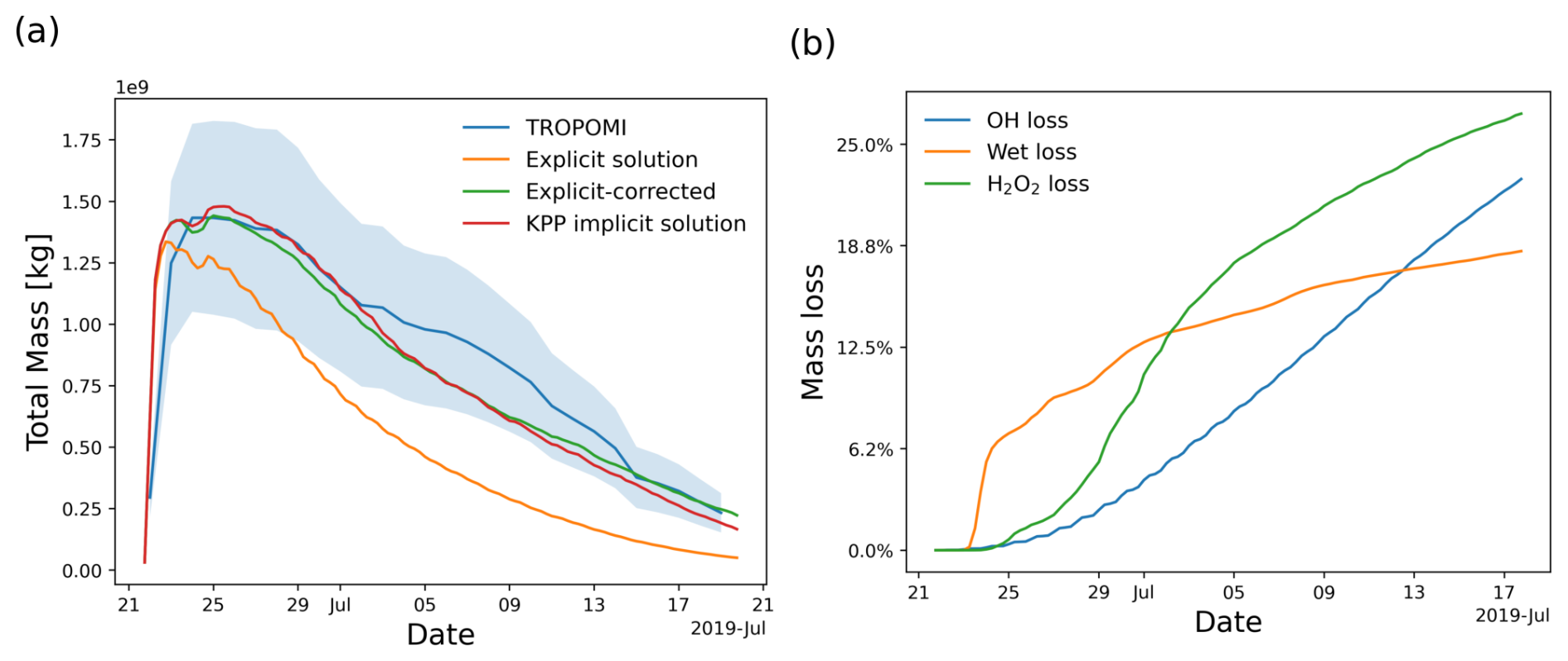
Figure 5 (a) Temporal evolution of the SO₂ total mass burden of the 2019 Raikoke eruption from TROPOMI measurements (blue curve, with the shading showing the uncertainty range) and MPTRAC simulations with the explicit solution (orange curve), the simplified explicit solution with correction (green curve), and the KPP implicit solution (red curve). (b) Estimates of the SO₂ total mass loss of the Raikoke eruption due to OH oxidation (blue curve), wet deposition (orange curve), and H₂O₂ oxidation (green curve) from the simplified explicit solution with correction.

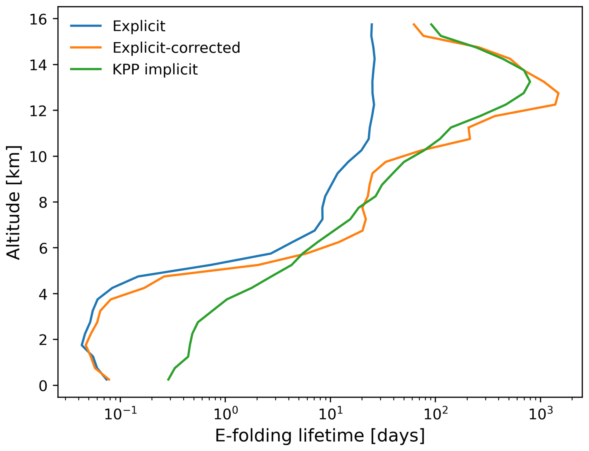
Figure 6 Vertical profiles of the average SO₂ e-folding lifetime of MPTRAC simulations with the explicit solution (green curve), the explicit solution with correction (orange curve), and the KPP implicit solution (blue curve) during the period from 25 June to 4 July.

The lifetime profile obtained with the KPP implicit solution indicates that the SO₂ has much longer lifetimes at higher altitudes. The lifetime is typically within a few hours to several days below an altitude of 5 km, whereas it exceeds 10 to 100 d above an altitude of 5 km. Due to the frequent presence of clouds in the lower and middle troposphere, SO₂ is taken up into the liquid phase and decays rapidly due to cloud-phase oxidation with H₂O₂ and wet deposition, leading to the shorter lifetime compared with the stratosphere. The vertical lifetime profile of the implicit KPP scheme shows a peak in the stratosphere that is not found in the explicit scheme. This is attributed to a reduction in the OH concentration within the SO₂ plume, which is captured by the implicit chemistry scheme but not by the explicit scheme, which uses a constant OH climatology.

While still within the uncertainty range of the TROPOMI observations, Fig. 5a highlights a notable discrepancy between the SO₂ total mass from TROPOMI and the MPTRAC simulations during 3–15 July 2019. The work of de Leeuw et al. (2021) attributed the change in SO₂ lifetime observed by TROPOMI about 10 d after the eruption to the removal of a large fraction of the tropospheric SO₂ mass through aqueous-phase oxidation and wet deposition. Beyond this point, the TROPOMI observations become dominated by the stratospheric component of the SO₂ cloud. As the stratosphere contains much less moisture, SO₂ removal occurs at a much lower rate, primarily through gas-phase reactions with OH, leading to significantly longer e-folding lifetimes. Our MPTRAC simulations are based on the SO₂ injection profiles provided by Cai et al. (2022), which may underestimate the stratospheric fraction and, consequently, impact on long-range transport. However, the estimates of SO₂ mass loss from the MPTRAC simulations (Fig. 5b) indicate a significant reduction in loss rates from wet deposition and H₂O₂ oxidation after 3 July. This aligns closely with the findings of de Leeuw et al. (2021).

3.3 Correction for the simplified explicit scheme

From Figs. 5 and 6, it can be seen that the simplified explicit approximation overestimates the SO₂ decay rate by ∼ 60 % compared with the TROPOMI observations, whereas the implicit KPP solution agrees well with the TROPOMI observations. Hence, there is also a ∼ 60 % difference between the explicit solution and the KPP solution. This overestimation in the explicit scheme is likely due to changes in OH and other radicals resulting from the SO₂ injection itself, which are not accounted for in the climatology. To account for that, we developed an SO₂-dependent correction to the OH climatology. Essentially, the simplification of the explicit scheme applies a linear approximation to describe the nonlinear oxidation processes. To compare the differences in lifetime of the two schemes, we performed another simulation without SO₂ injections to estimate the undisturbed background levels of OH and H₂O₂ and compared them with the conditions in the SO₂ plume. Figure 7 shows the ratio of the OH and H₂O₂ concentrations in the SO₂ plume versus the background oxidant concentrations as a function of the SO₂ VMR. The ratio decreases as the abundance of SO₂ increases, which means that the depletion of the oxidants is faster than their production. In highly concentrated SO₂ regions, the oxidants are almost completely depleted.

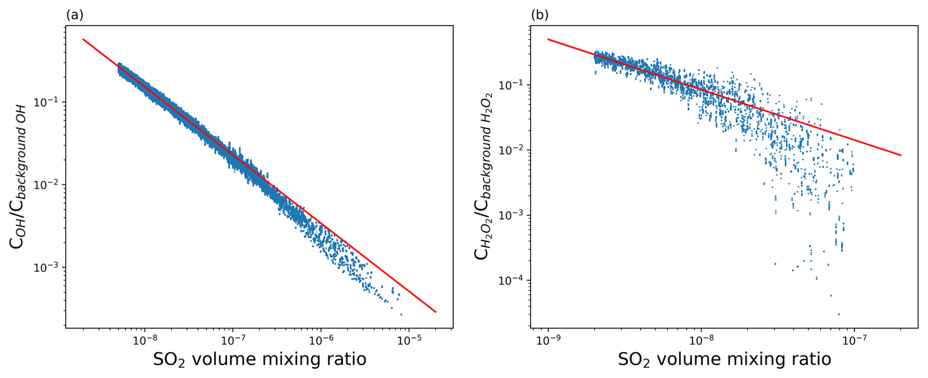
Figure 7 Ratio of the OH concentration in dry atmosphere (a) and the H₂O₂ concentration in cloud regions (b) in the Raikoke SO₂ plume versus background levels as a function of the SO₂ VMR. Each data point represents a single air parcel. The red lines represent the regression formulas given in Eqs. (3) and (4).

Note that the data points shown in Fig. 7 are filtered using a z-score threshold, as there are factors other than the chemical reactions that will affect the SO₂ distributions, such as diffusion, convection, and wet deposition, causing the data not to be statistically representative. After filtering outliers with low z scores, a correction formula to estimate OH concentrations in the plume from OH background levels and the SO₂ concentration can be obtained by regression:

$$\begin{array}{}\text{(3)}& \left[\mathrm{OH}\right]=\mathrm{4.72}\times {\mathrm{10}}^{-\mathrm{8}}[{\mathrm{SO}}_{\mathrm{2}}{]}^{-\mathrm{0.83}}\times [\mathrm{OH}{]}_{\mathrm{background}}.\end{array}$$

Similarly, the correction formula for H₂O₂ is

$$\begin{array}{}\text{(4)}& \left[{\mathrm{H}}_{\mathrm{2}}{\mathrm{O}}_{\mathrm{2}}\right]=\mathrm{3.13}\times {\mathrm{10}}^{-\mathrm{6}}[{\mathrm{SO}}_{\mathrm{2}}{]}^{-\mathrm{0.57}}\times [{\mathrm{H}}_{\mathrm{2}}{\mathrm{O}}_{\mathrm{2}}{]}_{\mathrm{background}}.\end{array}$$

By applying the corrections to the climatological OH and H₂O₂ data to account for their removal in the SO₂ plume, a simulation with the simplified explicit approximation with correction can be conducted. Figure 6 shows that, above an altitude of 10 km, the correction for the simplified explicit solution shifts the simulated lifetime closer to the KPP implicit solution. The correction reduces the amount of the oxidants when SO₂ is highly abundant in the volcanic plume. The mass evolution simulated by the corrected explicit solution is, therefore, in better agreement with the TROPOMI measurements and the KPP implicit solution (Fig. 5). These results reflect the fact that the chemical degradation of volcanic SO₂ is a nonlinear process, which means that it should not simply be treated as a pseudo-first-order reaction. The correction of the OH and H₂O₂ concentrations applied to the explicit solution improves the representation of SO₂ decay in the chemistry transport simulations, with almost no additional computational overhead.

3.4 Evaluation of the simulated OH field

The hydroxyl radical (OH) is an important oxidant in atmospheric chemistry, controlling the chemical decomposition of various species. For chemistry transport simulations of volcanic SO₂ in the UT–LS region, oxidation via OH is the main factor of mass decay in the gas phase. In order to simulate the OH background conditions during the Raikoke case study without any enhanced levels of volcanic SO₂ abundance with the chemical mechanism introduced in Sect. 2.2.2, we distributed a total of 1 million air parcels at altitudes between 9 and 17 km. The fourth-generation Copernicus Atmosphere Monitoring Service (CAMS) global reanalysis data (Inness et al., 2019) were then used for comparison with the OH field obtained with the implicit chemistry scheme implemented in MPTRAC. The CAMS reanalysis combines model data with observations using data assimilation techniques, providing a global distribution of atmospheric species. Key species assimilated in the CAMS reanalysis include ozone (O₃), carbon monoxide (CO), nitrogen dioxide (NO₂), methane (CH₄), and carbon dioxide (CO₂). Note that the hydroxyl radical (OH) and hydrogen peroxide (H₂O₂) are not directly assimilated from observations; instead, their concentrations are computed using the chemistry scheme implemented in the CAMS reanalysis.

Figure 8 compares zonal mean OH distributions at different pressure levels from the CAMS reanalysis, the MPTRAC model, and the CLaMS climatology. The best agreement among the three datasets is observed at the 100 hPa pressure level. Zonal mean OH concentrations increase gradually from near zero under polar winter conditions at high southern latitudes to approximately $\mathrm{2.5}\times {\mathrm{10}}^{-\mathrm{13}}$ ppv (parts per volume) in the northern subtropics. At northern middle and high latitudes, OH concentrations remain within 1.5 to $\mathrm{2}\times {\mathrm{10}}^{-\mathrm{13}}$ ppv. At lower vertical levels (150 to 250 hPa), differences of up to a factor of 2 are observed in the tropics and at northern middle to high latitudes. Overall, the CAMS and MPTRAC datasets tend to agree more closely with each other than with the CLaMS data. Differences in OH concentrations arise from variations in chemical mechanisms, emissions, meteorological conditions, photolysis schemes, spatial resolution, boundary conditions, and the representation of stratosphere–troposphere exchange processes.

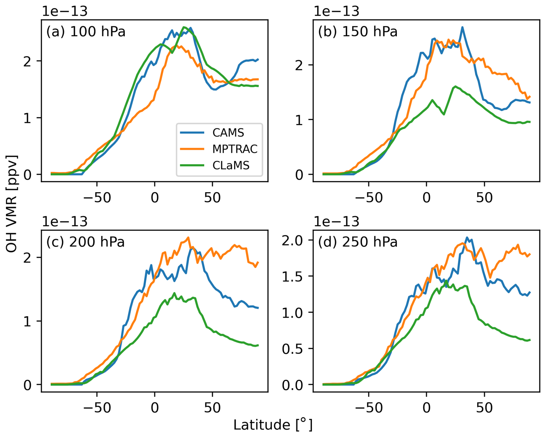
Figure 8 Zonal mean distributions of the OH field obtained from the CAMS reanalysis (blue curves), climatological data from the CLaMS model (green curves), and the MPTRAC simulation (orange curves) at pressure levels of 100 hPa (a), 150 hPa (b), 200 hPa (c), and 250 hPa (d) at 00:00 UTC on 1 July 2019.

Figure 9 shows the global CAMS and MPTRAC OH fields at pressure levels of 100 to 250 hPa at 00:00 UTC on 1 July 2019. The OH fields obtained by MPTRAC were generated using its implicit chemistry scheme under SO₂-free conditions. The MPTRAC OH fields exhibit similar spatial distributions with respect to the solar zenith angle dependence to the CAMS data, reflecting the strong correlation between OH production and solar radiation. The magnitudes of the OH concentrations produced by the two models are comparable, underscoring the reliability of MPTRAC with respect to capturing key OH dynamics.

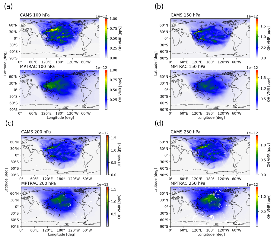
Figure 9 Global OH fields obtained from the CAMS reanalysis (top) and MPTRAC simulations (bottom) at pressure levels of 100 hPa (a), 150 hPa (b), 200 hPa (c), and 250 hPa (d) at 00:00 UTC on 1 July 2019.

A closer inspection reveals distinct features in the CAMS OH fields that are absent in the MPTRAC fields, such as localized OH plumes over Japan and the Pacific visible in the CAMS data. This discrepancy likely stems from the simplified oxidant mechanisms used in MPTRAC, which smooth out regional OH enhancements captured by CAMS. Additional factors, such as differences in spatial and temporal resolution and the representation of regional emissions and environmental conditions, further contribute to the observed differences. Despite these limitations, the MPTRAC scheme demonstrates a reasonable ability to simulate the production and loss of the short-lived OH radical in the UT–LS region, offering a practical balance between accuracy and computational efficiency for modeling SO₂ lifetimes in volcanic plumes and other atmospheric scenarios.

3.5 Selection of the chemistry time step

In MPTRAC, a fixed time step is applied for numerical integration of the trajectories and in most other modules. Based on previous studies (Rößler et al., 2018; Clemens et al., 2024), a time step of 180 s was selected for calculating trajectories with the midpoint method and considering the spatiotemporal resolution of the ERA5 reanalysis data. This choice of the time step provides a reasonable trade-off in terms of accuracy and the computational cost of the trajectory calculations (i.e., it is small enough to consider integration errors negligible while providing a minimum in computation time). In terms of computation effort, the time step of 180 s is acceptable for the explicit solution, but it is not efficient for the implicit chemistry calculations, which is particularly demanding in terms of computation.

To improve the computational efficiency for the implicit chemistry scheme, we implemented a distinct time step for the chemistry calculations. The chemistry time step is an important control parameter, as it has a significant impact on the computational efficiency. The chemistry time step size should be as large as possible without compromising the accuracy of the results. Figure 10 shows the temporal evolution of the SO₂ total mass obtained by different chemistry time steps. The results diverge when the time step of the chemistry calculations is larger than 6 h. Therefore, we recommend using a chemistry time step of 3 to 6 h to balance the computational efficiency and accuracy of the solution for the volcanic SO₂ oxidation.

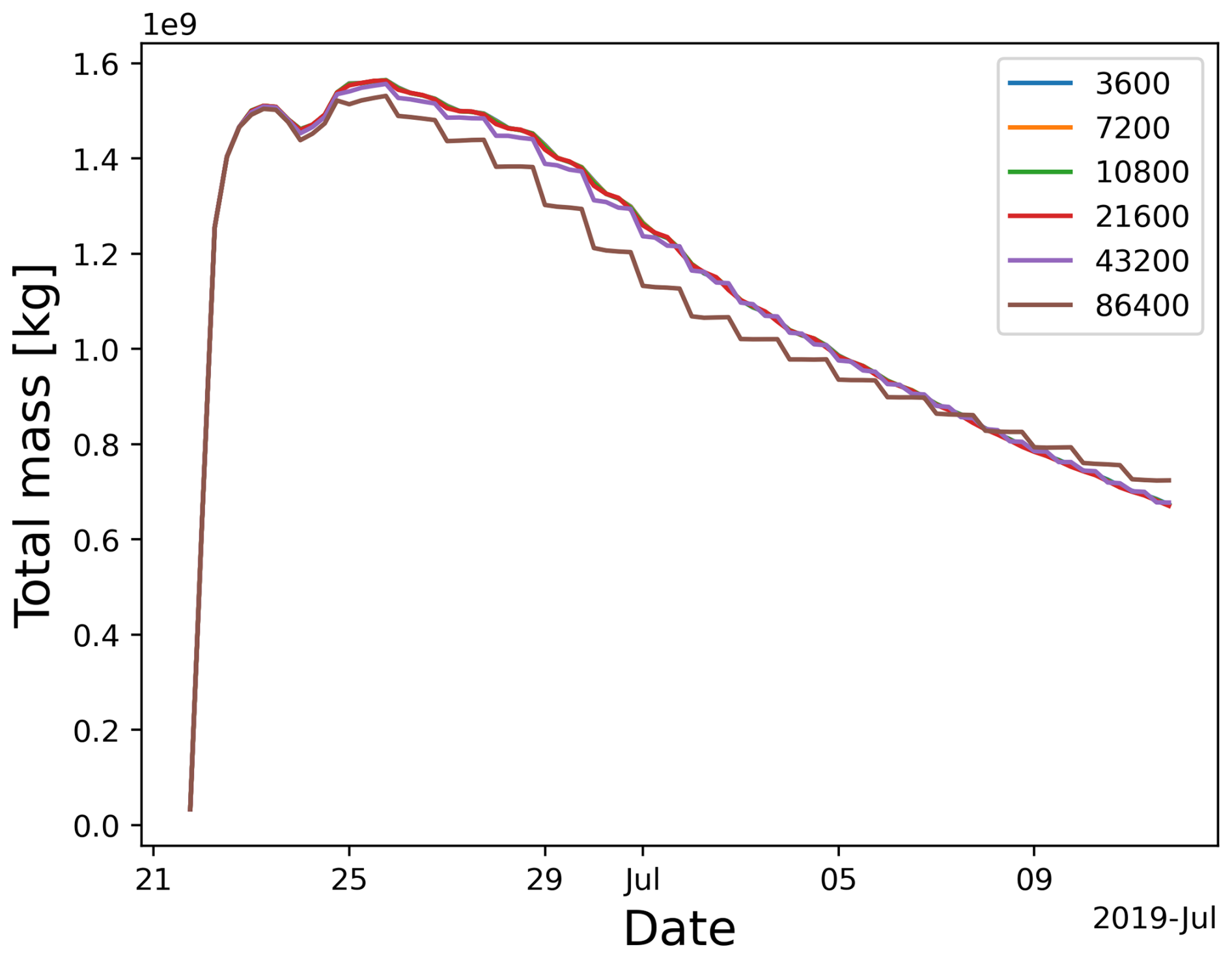
Figure 10 Total mass burden evolution simulated with different chemistry time step size settings of 3600, 7200, 10 800, 21 600, 43 200, and 86 400 s (see the legend).

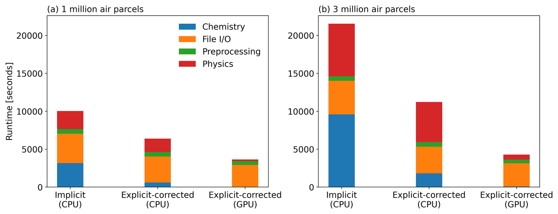
Figure 11 Computational cost of the Raikoke simulations with different chemistry schemes (the implicit scheme and the simplified explicit scheme with correction) on the JUWELS Cluster (CPU) and JUWELS Booster (GPU) for a simulation with 1 million air parcels on a scale of 1 million air parcels (a) and 3 million air parcels (b). The blue bar represents the runtime for the chemistry calculations, whereas the red bar represents the runtime for the other physical modules besides chemistry.

3.6 Assessment of computational costs

The KPP-based implicit chemistry solver implemented in MPTRAC can solve complex chemical mechanisms with a flexible definition of the chemical reactions and species. In the case of the volcanic SO₂ chemistry transport simulations, the corrected explicit solution achieves similar results with higher computational efficiency. For now, GPU offloading has been implemented using OpenACC for the simplified explicit scheme, whereas this is planned for the future for the implicit scheme. Figure 11 shows the runtime of MPTRAC simulations on the JUWELS supercomputer at the Jülich Supercomputing Centre comparing the implicit and explicit chemistry schemes using a chemistry time step of 21 600 and 180 s, respectively. The CPU simulations were conducted on a single compute node of the JUWELS Cluster (Jülich Supercomputing Centre, 2019), parallelized with 48 OpenMP threads. Each compute node of the JUWELS Cluster contains two Intel Xeon Platinum 8168 CPUs with 24 physical cores per CPU. The GPU simulations were conducted on the JUWELS Booster (Jülich Supercomputing Centre, 2021) with two AMD EPYC Rome 7402 CPUs and four NVIDIA A100 GPUs per node.

Regarding the chemistry, Fig. 11a shows that the simplified explicit solution is about 5.3 times faster than the KPP implicit solution for a simulation with 1 million air parcels. Considering that file input/output (I/O) and meteorological data preprocessing also require a substantial part of the total runtime, the total runtime is reduced by ∼ 56 % by choosing the more efficient explicit chemistry scheme. The GPU solution of the simplified explicit chemistry scheme on the JUWELS Booster reduces the total runtime by ∼ 75 %, with the runtime required for chemistry becoming nearly negligible. As the scale of the simulation increases (i.e., for simulations with more air parcels), the advantage of the explicit solution in terms of computational efficiency becomes even more pronounced. Figure 11b shows that the total runtime is reduced by 92 % for a simulation with 3 million air parcels. This improvement in computational efficiency is particularly relevant for large-scale chemistry transport simulations, where finding the proper trade-off between accuracy and computational cost is most critical. In the future, the KPP implicit scheme might also be equipped with GPU offloading to improve its performance (Alvanos and Christoudias, 2017; Christoudias et al., 2021).

4 Summary and conclusions

The MPTRAC Lagrangian transport model offers two schemes for simulating SO₂ chemistry in volcanic eruptions: (1) an explicit approach utilizing climatological data for reaction rates and SO₂ decay and (2) an implicit approach leveraging KPP's Rosenbrock integrator for multi-species chemical processes. KPP can solve complex chemical mechanisms with a flexible definition of chemical species, reactions, and rate coefficients. The implicit solution allows for more complex, nonlinear chemical mechanisms with dynamic reaction rates depending on the species concentrations. Here, we propose a chemical mechanism with 31 reactions and 12 species to model the production and loss of the short-lived OH radical and H₂O₂, which are essential for the decomposition of SO₂ in the gas and aqueous phase, respectively, in the UT–LS region. The mechanism proposed here can serve as a basis for developing more complex chemical mechanisms in future studies. It could also be further optimized by evaluating the relevance of each reaction pathway to reduce the computational effort.

The OH radical is the main oxidant in the gas phase, which largely controls the decomposition of SO₂ in the UT–LS. We compared OH radical fields obtained by the proposed mechanism in MPTRAC with CAMS reanalysis data and climatological data from the CLaMS model. The OH radical field obtained by the proposed mechanism shows a clear characteristic of diurnal variation and concentrations at a similar level compared to these reference datasets. The cloud-phase H₂O₂ oxidation also has a significant impact on the SO₂ decay in the lower troposphere. It must be taken into account to properly represent the loss of tropospheric SO₂ over time, especially for other volcanic eruptions, such as those happening in the tropics with lower peak emission heights (Liu et al., 2023). Cloud-phase oxidation has been considered in all cases in this study.

Applying the chemical mechanisms to the June 2019 Raikoke eruption, the implicit KPP-based solution aligns well with TROPOMI satellite data on SO₂ mass burden evolution, whereas the simplified explicit approach overestimates SO₂ decay by 60 %. This overestimation is due to using the OH and H₂O₂ climatological background field without considering enhanced levels of SO₂. Regression-derived correction formulas for OH and H₂O₂ concentrations (y=ax^b) adjust climatology-based oxidant levels, introducing nonlinear effects that enhance SO₂ lifetime representation in explicit simulations. We also applied the correction to another volcanic eruption, the July 2018 Ambae eruption (Liu et al., 2023), and observed that it produced a total SO₂ lifetime comparable to that predicted by the KPP implicit solution. Notably, despite differences in the geographic and atmospheric condition – Ambae is situated in the tropics and Raikoke is located in the midlatitudes – the same parameter values for a and b in the correction formula were used. This suggests that the correction approach is transferable across diverse eruption scenarios.

The corrected explicit solution achieves realistic lifetime modeling with more than 5 times the efficiency of the implicit approach, making it ideal for computationally demanding applications, such as emission reconstruction through inverse modeling. Previous studies using backward-trajectory methods for volcanic SO₂ lacked realistic chemical lifetime modeling, a limitation now being addressed. Ongoing development includes inverse modeling techniques for source estimation, incorporating support for nonlinear chemical mechanisms, and investigating the interplay between lifetime modeling and source reconstruction. These advancements significantly enhance MPTRAC’s Lagrangian chemistry modeling capabilities, enabling more precise source estimation and positioning the model for broader applications on modern HPC systems.