Age of air from ACE-FTS measurements of sulfur hexafluoride

Climate models predict that the Brewer–Dobson circulation (BDC) will accelerate due to tropospheric warming, leading to a redistribution of trace gases and, consequently, to a change of the radiative properties of the atmosphere. Changes in the BDC are diagnosed by the so-called “age of air”, that is, the time since air in the stratosphere exited the troposphere. These changes can be derived from a long-term observation-based record of long-lived trace gases with increasing concentration in the troposphere, such as sulfur hexafluoride (SF₆). The Atmospheric Chemistry Experiment Fourier Transform Spectrometer (ACE-FTS) provides the longest available continuous time series of vertically resolved SF₆ measurements, spanning 2004 to the present. In this study, a new age-of-air product is derived from the ACE-FTS SF₆ dataset. The ACE-FTS product is in good agreement with other observation-based age-of-air datasets and shows the expected global distribution of age-of-air values. Age of air from a chemistry–climate model is evaluated, and the linear trend of the observation-based age of air is calculated in 12 regions within the lower stratospheric midlatitudes (14–20 km, 40–70°) in each hemisphere. In 8 of 12 regions, there was not a statistically significant trend. The trends in the other regions, specifically 50–60 and 60–70° S at 17–20 km and 40–50° N at 14–17 and 17–20 km, are negative and significant to 2 standard deviations. This is therefore the first observation-based age-of-air trend study to suggest an acceleration of the shallow branch of the BDC, which transports air poleward in the lower stratosphere, in regions within both hemispheres.

1 Introduction

While it is well known that increased greenhouse gas concentrations are causing a warming of the troposphere and a cooling of the stratosphere, so far few observational datasets have constrained how this affects the Brewer–Dobson circulation (BDC). The BDC is characterized by poleward motion in the stratosphere through two distinct branches (Plumb, 2002; Birner and Bönisch, 2011). The shallow branch transports air from the tropics to higher latitudes in the lower stratosphere (below ∼ 20 km), with transit timescales on the order of months to a couple of years. The deep branch brings air poleward during the winter at higher altitudes, with transit timescales on the order of more than 2 years. Model studies suggest that both branches of the BDC are accelerating (e.g., Butchart, 2014, and references therein), but this has been difficult to confirm with measurements.

The speed of the BDC cannot be measured directly, so it must be inferred from other quantities. One way to do this is to estimate the “age of air”, that is, the time that has passed since air left the troposphere (Waugh and Hall, 2002). Since air typically enters the stratosphere through tropical upwelling and is then subjected to the BDC as it moves poleward, this definition of age of air is a useful indicator of BDC-related mean transport time. At a particular location, younger ages correspond with shorter transit times, while older ages correspond with longer transit times. It is also necessary to address the fact that any finite region under consideration (that is, a macroscopic “air parcel”) is made up of air of different ages. The distribution of these ages is referred to as the age spectrum (Hall and Plumb, 1994), which can be modelled as an inverse Gaussian function with a mean (i.e., the mean age of stratospheric air) and a width. Mixing between air parcels leads to wider age spectra, as it increases the number of different pathways leading to a specific location. A decrease in the mean age of air at higher latitudes, with no change in the tropics, indicates a decrease in the mean transport time from the tropics to higher latitudes and therefore an acceleration of the BDC (e.g., Neu and Plumb, 1999; Linz et al., 2016, 2017). This motivates the need for trend detection in age of air derived from observations.

Age of air can be estimated from long-lived trace gases that have increasing concentrations in the troposphere, also known as “clock” tracers. Once an air parcel containing such a gas enters the stratosphere, the volume mixing ratio (VMR) does not change due to the absence of chemical sinks (hence the long lifetime), and the concentration is therefore an indicator of when the parcel left the troposphere. CO₂, fluorocarbons, and hydrofluorocarbons are some commonly used clock tracers, but one of the most often used is SF₆, which according to surface measurements (e.g., Levin et al., 2010; Rigby et al., 2010; Simmonds et al., 2020) has been steadily increasing in the troposphere since the mid-20th century due to industrial activity. It has effectively no seasonal cycle or stratospheric sinks, which complicate the use of CO₂ and chlorofluorocarbons (CFCs) for similar analyses. However, SF₆ is destroyed in the mesosphere via photolysis and electron-capture reactions (Morris et al., 1995; Reddmann et al., 2001; Totterdill et al., 2015).

There are several aircraft- and balloon-borne in situ measurements of SF₆ available from the last 3 decades that have been used to infer age of air (e.g., Volk et al., 1997; Engel et al., 2002). Those that were used in this study are highlighted here. Harnisch et al. (1996) calculated age of air using cryosampler measurements of SF₆ from the AIRE 93 and SESAME 95 balloon flights over France (44° N) in September 1993 and Sweden (68° N) in March 1995, respectively. Andrews et al. (2001) derived age of air from SF₆ measured by the LACE instrument on board three balloon flights over the USA (35 and 65° N) and Brazil (7° S) throughout 1996 and 1997. For that study, age of air was also derived using NASA ER-2 aircraft-based SF₆ measurements taken by the ACATS-IV instrument between 1992 and 1997. The former two studies also derived age of air using CO₂ measurements taken during the same campaigns, and Boering et al. (1996) did so using CO₂ measurements from these ER-2 flights. More recently, Leedham Elvidge et al. (2018) and Adcock et al. (2021) calculated age of air using SF₆ measurements based on whole-air samples taken during M55 Geophysica high-altitude aircraft flights. The former used one campaign over Germany in October–November 2009 (48–54° N) alongside two campaigns over Sweden (62–77° N) in January–February 2010 and December 2011. The latter involved one campaign over Greece (33–41° N) in September 2016 and another over Nepal (21–29° N) in July–August 2017. Both studies also determined an “averaged age of air” using measurements of multiple other clock tracers besides SF₆ taken during the same campaigns.

The only vertically resolved global age-of-air dataset currently available is derived from MIPAS (Michelson Interferometer for Passive Atmospheric Sounding) measurements of SF₆ and spans the 2002–2012 period (Stiller et al., 2008, 2012; Haenel et al., 2015). This spatially and temporally dense satellite dataset has been invaluable in age-of-air studies, but the relatively short time series makes trend detection challenging. Hardiman et al. (2017) used model simulations to determine that natural variability could mask changes in the BDC for a time series shorter than 12 years, like that available from MIPAS. This motivates the development of a new satellite-based age-of-air dataset using ACE-FTS (Atmospheric Chemistry Experiment Fourier Transform Spectrometer), which provides the longest available time series of vertically resolved global SF₆ measurements. In this study, ACE-FTS retrievals of SF₆ were used to calculate age of air for the February 2004–February 2021 period.

Several studies have used existing measurement-based age-of-air datasets as well as reanalysis data to evaluate model predictions regarding the acceleration of the BDC. Engel et al. (2009) compiled age of air derived from balloon-borne cryosampler measurements of CO₂ and SF₆ in the northern midlatitude stratosphere (24–35 km) from 1975–2005 into a single time series. Over this 30-year period, a slight positive but statistically insignificant change was detected. Additional balloon data taken in 2015 and 2016 were added to this time series and resulted in an even smaller and still statistically insignificant positive trend (Engel et al., 2017). Bönisch et al. (2011) identified a change in the slopes of O₃–N₂O correlations using aircraft-based in situ measurements taken between 1979 and 2009. This was linked to increased upwelling in the tropics, a potential sign of acceleration of the BDC. Within the same study, the observation was corroborated with Japanese 25-year Reanalysis data (Onogi et al., 2007), which showed a 1-month-per-decade decrease in transit times into the midlatitude lower stratosphere, suggesting a slight acceleration of the shallow branch. However, the same reanalysis data indicated that the deep branch did not accelerate over this time period. Diallo et al. (2012) also used reanalysis data, from ERA-Interim, to calculate the trend in age of air for the 1989–2010 period. A significant negative trend of 3.5–6 months per decade was found in the southern (and northern equatorward of 40° N) lower stratosphere, but no clear trend was detected in the mid-stratosphere. This also suggests that the shallow branch of the BDC is accelerating, while there is no clear trend in the deep branch. Ray et al. (2014) used an idealized model constrained by balloon-borne in situ measurements of SF₆ and CO₂ to assess variability in Northern Hemisphere age of air and identified a negative trend in the lowest 5 km of the stratosphere but a positive trend at higher altitudes. Haenel et al. (2015) found similar results in trends based on the MIPAS age-of-air dataset: negative trends in the lowermost tropical and southern midlatitude stratosphere but positive trends in the northern midlatitudes and at both poles, all on the order of a few months to a year per decade. The persistent finding across these studies is that while there is no clear signal (in observations or reanalyses) that the BDC is accelerating as a whole, the shallow branch in the Southern Hemisphere does appear to have accelerated.

This study details the development of the ACE-FTS age-of-air dataset as follows. Section 2 describes the ACE-FTS and MIPAS SF₆ datasets, which are compared with each other and with in situ SF₆ measurements in Sect. 3. Section 4 provides an explanation of how age of air was calculated from ACE-FTS SF₆ measurements, taking into account the complication arising from the sink due to photolysis in the mesosphere. The ACE-FTS age-of-air results are presented in Sect. 5. These include an exploration of the effects of the mesospheric sink correction, comparisons with age of air previously derived from in situ and newly derived from MIPAS measurements, a comparison with age-of-air output from a specified dynamics (nudged) simulation with the Canadian Middle Atmosphere Model (CMAM39), and the calculation of trends in age of air for the 2004–2021 period.

2 Satellite datasets

The focus of this study is mean age of stratospheric air (hereafter referred to as simply “age of air”) based on SF₆ measurements from ACE-FTS, for which age of air is calculated for the first time. An updated age-of-air product based on MIPAS data is also presented, since the details of the method for age-of-air calculation have evolved since Stiller et al. (2012) and Haenel et al. (2015).

2.1 ACE-FTS

ACE-FTS is a high-spectral-resolution (0.02 cm⁻¹) infrared Fourier-transform spectrometer on board the satellite SCISAT that has been taking measurements since February 2004 (Bernath et al., 2005). It is a solar occultation instrument; the concentrations of atmospheric gases are determined by fitting their known absorption spectra to the spectra obtained during each sunrise or sunset. The retrieval algorithms for versions 3 and 4 are described in detail in Boone et al. (2013) and Boone et al. (2020), respectively. During each occultation, ACE-FTS takes measurements at various altitudes, supplying a profile with 2–3 km vertical resolution which is provided on a 1 km grid. From an orbital inclination of 74°, ACE-FTS measurements reach up to 85° in each hemisphere. It has been making up to 30 occultations per day (2 per orbit) since early 2004, compiling a dataset that contains over 100 000 profiles concentrated at higher latitudes. The vertical coverage of these profiles ranges from 6 to 150 km depending on the gas. Due to the nature of solar occultation measurements, ACE-FTS has limited sampling. It takes 3 months for ACE-FTS to obtain global coverage, and the measurements are not distributed evenly in latitude throughout each month. This must be taken into consideration when comparing ACE-FTS with other instruments or with models, usually by subsampling the larger dataset and finding coincident measurements.

Despite the relative sparsity of ACE-FTS measurements when compared with other satellite instruments, the ACE-FTS orbital pattern and retrieval method offer several advantages for this study. The first is that solar occultation measurements have a higher signal-to-noise ratio than measurements of atmospheric emission, which is particularly useful for a gas like SF₆ with such a low VMR (i.e., a few parts per trillion). Additionally, the deep branch of the BDC is imprinted in downwelling over polar regions, so age of air at higher latitudes is of interest for inferring changes related to this. The ACE-FTS sampling pattern is suited for this purpose as nearly 50 % of profiles are taken poleward of 60°. Most importantly, the 17-year time series of consistent SF₆ measurements is unmatched by previous datasets. The lack of measurement density does present a challenge, but the advantages of using ACE-FTS for age-of-air studies far outweigh this difficulty.

Here, two versions of ACE-FTS were considered: v3.5/3.6 (February 2004–February 2021) and v4.1/4.2 (February 2004–present). ACE-FTS v3.5/3.6 was included because the retrieval update for v4 resulted in an unphysical feature in SF₆ between 18 and 30 km. The same issue has been observed in the current ACE-FTS dataset, v5.2. The ACE-FTS data are accompanied by a set of quality flags that indicate whether a measurement is recommended for use. The flags for v4 are provided separately by Sheese and Walker (2020), and for v3, the flags are included in the ACE-FTS VMR files. These quality flags were developed by Sheese et al. (2015), and they were employed as recommended, keeping only measurements with a flag of 0 and removing entire profiles that contained at least one measurement with a flag of 4 or 5. There is a drift in v3 known to affect ozone and temperature profiles, and potentially others, that was corrected for in v4 (Boone et al., 2020).

2.2 MIPAS

MIPAS was a Fourier-transform spectrometer on the Envisat satellite that measured infrared limb emission spectra from July 2002 to April 2012 (Fischer and Oelhaf, 1996; Fischer et al., 2008). Technical problems in 2004 caused a reduction in spectral resolution from 0.025 to 0.0625 cm⁻¹ (unapodized) but a 20 % increase in the number of measured profiles starting in January 2005. Envisat was in a Sun-synchronous orbit with an inclination of 98.55° and an altitude of 800 km, completing nearly 15 revolutions per day and about 100 scans per orbit, amounting to approximately 1500 profiles per day. Scans were taken at 10:00 or 22:00 local solar time (LST) and covered 87° S–89° N. The profiles are provided on a uniform altitude grid from 6 to 70 km. The SF₆ retrievals are done by the Institut für Meteorologie und Klimaforschung (IMK) together with the Instituto de Astrofísica de Andalucía (IAA) and are described in von Clarmann et al. (2003), with the changes made for the reduced resolution period explained in von Clarmann et al. (2009). In this study, the lower-resolution SF₆ measurements from version 5 (V5R) (Haenel et al., 2015) were used to maximize temporal coverage while using a single dataset. Specifically, V5R_222 and V5R_223 were used because they are the most recent SF₆ products that were retrieved using the same spectroscopic parameters (Varanasi et al., 1994) as versions 3 and 4 of ACE-FTS. As recommended by the instrument team, all SF₆ measurements with a visibility flag of 0 and averaging kernel diagonal less than 0.03 were removed.

SF₆ and derived age of air from MIPAS were both considered for comparison purposes. To account for the difference in measurement density between MIPAS and ACE, the comparisons between the two were done using both the full MIPAS V5R dataset and a subsampled version that only contains measurements which are coincident with an ACE-FTS measurement. MIPAS V5R SF₆ measurements were sampled onto the ACE-FTS grid by, for each ACE-FTS measurement, finding the closest MIPAS measurement that is within 12 h and 1000 km and on the same side of the polar vortex edge (i.e., both are inside, both are outside, or both are inside the edge). The polar vortex edge is defined as any point where the absolute value of scaled potential vorticity (sPV; e.g., Dunkerton and Delisi, 1986; Manney and Zurek, 1993; Manney et al., 1994) is between $\mathrm{1.2}\times {\mathrm{10}}^{-\mathrm{4}}$ and $\mathrm{1.6}\times {\mathrm{10}}^{-\mathrm{4}}$ s⁻¹. Lower sPV values are considered to be outside the vortex, while higher values are considered to be inside the vortex. For this step, each altitude was considered separately, meaning that one profile could include some measurements inside the vortex and some measurements outside the vortex. sPV values at the ACE-FTS and MIPAS measurement locations were taken from the Jet Propulsion Laboratory derived meteorological products (JPL DMPs, Manney et al., 2007, 2011; Millán et al., 2023), which are based on NASA's Global Modeling and Assimilation Office's MERRA-2 (Modern-Era Retrospective analysis for Research and Applications) (Gelaro et al., 2017). The generous 1000 km coincidence criterion for distance was chosen to maximize the number of coincidences; using stricter coincidence criteria did not significantly improve the comparisons. Approximately half the ACE-FTS measurements over the relevant time period had a coincident MIPAS measurement.

3 SF₆ comparisons

Prior to this study, ACE-FTS SF₆ measurements (version 3.0) had only been compared with output from the SLIMCAT 3D chemical transport model, with good agreement found at all altitudes between 12 and 33 km (Brown et al., 2011). Here, comparisons of mean profiles from ACE-FTS v3.5/3.6 and v4.1/4.2 for the tropics (20° S–20° N), the extratropics (20° up to polar vortex edge, $\left|\mathrm{sPV}\right|<\mathrm{1.2}\times {\mathrm{10}}^{-\mathrm{4}}$ s⁻¹), and the polar vortex ($\left|\mathrm{sPV}\right|>\mathrm{1.6}\times {\mathrm{10}}^{-\mathrm{4}}$ s⁻¹) are shown in Fig. 1. The same occultations were used from each version for these comparisons. The error bars represent 1 standard error of the mean at each altitude. The v4.1/4.2 profiles, shown in dark blue (solid), have a decrease in SF₆ near 18 km accompanied by a slight increase just above (indicated by the black arrows). This artefact is a result of how altitudes are determined in the retrieval (Chris D. Boone, personal communication, 2024). The previous version, v3.5/3.6, which is shown in light blue (solid), does not have this feature and was therefore chosen for this study. It should be noted that the decrease in SF₆ below about 14 km is caused by the fact that the altitude of the lowest retrieval varies over the course of the year. Therefore, the low-altitude bins can be missing measurements from certain times of year, resulting in this feature. Hereafter, “ACE-FTS” refers to v3.5/3.6. Comparisons with other SF₆ datasets are presented in the following section.

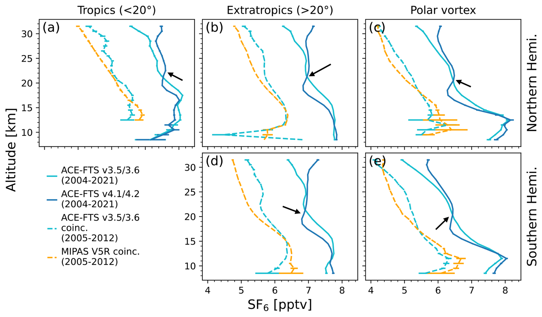
Figure 1 Mean profiles of SF₆ retrievals from ACE-FTS v3.5/3.6 (light blue), ACE-FTS v4.1/4.2 (dark blue), and coincident measurements from ACE-FTS v3.5/3.6 and MIPAS V5R (dashed light blue and dashed orange, respectively) for (a) the tropics (20° S–20° N), (b) the northern extratropics (north of 20° N and absolute sPV less than $\mathrm{1.2}\times {\mathrm{10}}^{-\mathrm{4}}$ s⁻¹), (c) the northern polar vortex (absolute sPV greater than $\mathrm{1.6}\times {\mathrm{10}}^{-\mathrm{4}}$ s⁻¹), (d) the southern extratropics (south of 20° S and absolute sPV less than $\mathrm{1.2}\times {\mathrm{10}}^{-\mathrm{4}}$ s⁻¹), and (e) the southern polar vortex (absolute sPV greater than $\mathrm{1.6}\times {\mathrm{10}}^{-\mathrm{4}}$ s⁻¹). Error bars represent the standard error of the mean. The black arrows indicate the artefact (see text) in SF₆ in v4.1/4.2.

3.1 Comparisons with MIPAS and in situ data

Figure 1 also shows profile comparisons of coincident ACE-FTS and MIPAS measurements averaged over 2005–2012 as dashed light-blue and dashed orange lines, respectively. In all regions, particularly outside the polar vortex, SF₆ decreases more rapidly with height in the stratosphere in the MIPAS measurements. The difference between the mean profiles is greatest in the extratropics, where ACE-FTS VMRs are greater than MIPAS by up to about 10 %. Within the polar vortex, SF₆ decreases to about 4.5 pptv at 30 km in both datasets, but the vertical gradients between 20 and 30 km differ. The MIPAS profile decreases more quickly from 20–25 km, but the ACE-FTS profile decreases more quickly from 25–30 km until the profiles meet again near 30 km. The largest differences, about 10 %, are at 24–25 km. It is also noteworthy that there is a difference of about 1 pptv between the ACE-FTS profile from the full dataset (2004–2021) and that from only measurements that are coincident with MIPAS (2005–2012). NOAA marine boundary layer (MBL) reference SF₆ (Global Monitoring Laboratory, 2023) increased from about 6.5 to 7.5 pptv between 2008 and 2012 (the midpoints of the two time periods), which accounts for the discrepancy. This reinforces the importance of using coincident measurements when comparing observations from two different instruments; comparing the full ACE-FTS mission with the full MIPAS mission would introduce significant bias due to the two different time periods. The mean profile from the full MIPAS mission is similar to that from the sampled MIPAS dataset and is not shown because it makes the comparison between the mean coincident profiles more difficult to visualize.

ACE-FTS and MIPAS SF₆ were also compared with balloon-borne profiles from the BONBON cryosampler (e.g., Engel et al., 2006; Laube et al., 2010). There were three flights available during the ACE-FTS mission: two over Brazil near 5° S on 8 and 25 June 2005 (B42 and B43) and one over Sweden near 67° N on 10 March 2009 (B45). Following Kolonjari et al. (2024), where ACE-FTS measurements were compared with B42 and B43, the coincidence criteria for these comparisons were quite broad: within 90 d and within 5° latitude, with no restriction on longitude. This ensured that there would be a sufficient number of coincidences even though ACE-FTS profiles are sparse in the tropics, particularly in June when the satellite's beta angle is high. Using these criteria, the B42 and B43 measurements were each coincident with 20–35 ACE-FTS measurements and up to over 2000 MIPAS measurements, depending on the altitude. The B45 measurements had over 400 coincident ACE-FTS measurements and over 8000 coincident MIPAS measurements.

The SF₆ values from each flight were compared with the means of coincident ACE-FTS or MIPAS measurements, shown in Fig. 2. The error bars represent 1 standard deviation. The agreement between all three datasets is excellent; the VMRs are consistent everywhere except near 21–23 km for flight B45 in Kiruna, where the balloon measurements are lower than the ACE-FTS measurements by about 15 %. This flight intersected with the polar vortex, which could cause a sharp decrease in SF₆ like that seen in this altitude region. Because of the necessarily broad definitions for coincidence, it is not expected that the satellite data show this isolated dynamical feature. Despite this, the comparison was included due to the limited availability of balloon-based SF₆ profiles for reference during the ACE-FTS measurement period.

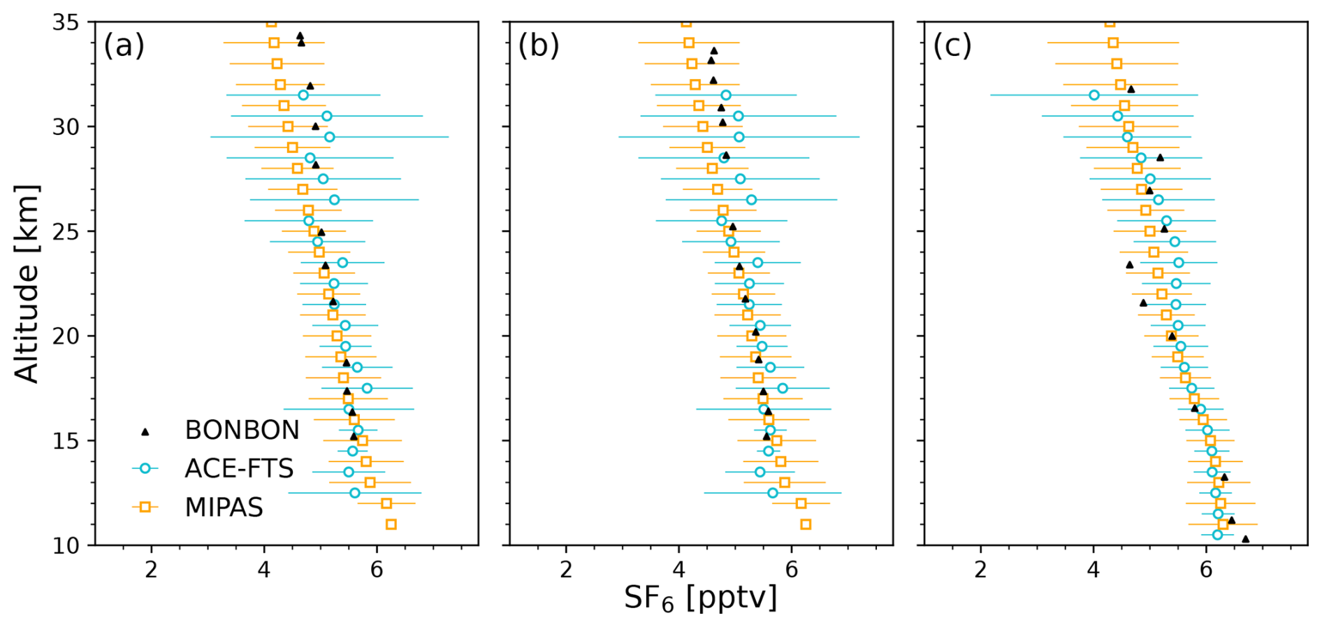
Figure 2 SF₆ profiles from three BONBON balloon flights (black triangles) on (a) 8 June 2005 (B42) and (b) 25 June 2005 (B43), both over Brazil near 5° S, and on (c) 10 October 2009 over Sweden near 68° N (B45). Also shown are means of SF₆ profiles from ACE-FTS (blue circles) and MIPAS (orange squares) that are within 90 d and 5° latitude of each BONBON profile. The error bars represent 1 standard deviation.

Overall, there is good consistency between the ACE-FTS SF₆ profiles and the MIPAS and BONBON datasets. ACE-FTS and MIPAS agree within 10 % in all latitude regions, and coincident profiles from both datasets agree within 1 standard deviation with the BONBON profiles.

4 Methodology for deriving age of air

The convolution method described in Garny et al. (2024b), slightly updated since Stiller et al. (2012) and Haenel et al. (2015), was used to infer age of air from SF₆ measurements. An overview of the method is provided here. For consistent comparisons, MIPAS age of air was recalculated for this study using the updated method. To reduce noise, the satellite instrument datasets were first zonally averaged by month, separately for each year (i.e., each bin corresponds to 1 month in 1 year). For most of this study, 10° latitude bins (centred on 85, 75° S, …, 85° N) and 3 km altitude bins (centred on 9.5, 12.5, …, 30.5 km) were used. In addition, a dataset with 5° latitude bins and one 2 km altitude bin from 19–21 km was also created for comparison purposes. There is also an age-of-air product provided using 10° equivalent latitude bins based on the equivalent latitude provided as part of the JPL DMPs. Similarly to the ACE-FTS climatologies described in Koo et al. (2017), at least five measurements were required in each bin (defined by month, year, latitude, and altitude). The mean SF₆ value in each bin was then used to calculate mean age of air; essentially, each bin was treated as an “air parcel”.

4.1 Tropospheric SF₆ reference time series

Since age of air is roughly defined as the time since an air parcel left the troposphere, a tropospheric SF₆ time series is required as a reference to match the parcel's SF₆ VMR with a tropospheric value and time. Specifically, a tropical tropospheric reference time series is needed as it is assumed that most air enters the stratosphere in the tropics. Such a time series is only available from surface measurements, so the age-of-air calculation includes a small correction to account for the difference between air at the surface and air at the tropopause (see below). The time series used here is made from a combination of datasets. Of most importance are the tropical NOAA MBL reference data, which were used from mid-1995 onward. For an accurate calculation, the reference time series should extend back about 15 years from the earliest stratospheric SF₆ value to allow for the detection of old air. In previous studies (e.g., Stiller et al., 2008, 2012; Haenel et al., 2015), the time series was linearly extrapolated to obtain values for earlier years. Here, the time series was extended back to 1989 using scaled monthly data from Cape Grim in Tasmania (Ray et al., 2014).

4.2 Surface correction

The age-of-air calculation uses surface SF₆ measurements as a tropospheric reference, but to find the time since entering the stratosphere, the stratospheric SF₆ VMRs should be compared with VMRs at the tropical tropopause. While SF₆ concentrations are not expected to decrease significantly from the surface to the tropopause since the transit timescale is on the order of weeks or months at most, a more accurate age can be calculated if the satellite data are corrected to account for this difference. Further, any measurement bias between the ground-based data and the satellite observations can be detected and corrected for by this method.

This was done by finding a bias correction that shifts the tropical tropospheric ACE-FTS values to the reference time series values and applying it to all ACE-FTS measurements. The tropics were defined to be those profiles between 17.5° S and 17.5° N, for consistency with Stiller et al. (2012) and to avoid influence from the extratropics. The troposphere was defined as those measurements that are at least 2 km below the WMO tropopause, which is another JPL DMP calculated for each ACE-FTS profile. This was to reduce the influence of troposphere-stratosphere mixing in the upper troposphere and therefore ensure that only the well-mixed portion of the troposphere was included. This correction also accounts for instrument bias and for the possibility of a satellite measurement detecting both tropospheric and stratospheric air due to coarser vertical resolution. If the satellite VMRs are too low relative to the reference time series, for example, then ages calculated based on the reference time series will be too high. Ensuring agreement between the two datasets in the troposphere reduces the influence of these biases.

The monthly tropical tropospheric SF₆ means from ACE-FTS are shown as blue circles in Fig. 3a along with the reference time series (black line). There is good agreement, mostly within ±5 %, but after 2014, the majority of ACE-FTS measurements fall below the reference time series. The differences could be due to changes in measurement density, which increased over time, or the known drift in v3.5/3.6 retrievals. This discrepancy further motivates a correction to the ACE-FTS measurements. The relative differences between monthly mean tropical tropospheric SF₆ from ACE-FTS and the surface monthly means are shown in Fig. 3b. A cubic least-squares fit, shown by the red line, was used to find the relative bias r_t for each month of the time series. Linear and quadratic fits resulted in noticeable structure in the fit residuals, so a cubic fit was chosen. Figure 3c shows the reference time series and the corrected ACE-FTS tropical tropospheric values (blue squares). The corrected time series was calculated by dividing each VMR in the time series by 1+r_t. The corrected ACE-FTS values no longer drift relative to the reference time series after 2014. The correction was applied to all ACE-FTS SF₆ climatological means based on month and year but not based on latitude or altitude, since latitude and altitude dependence cannot be determined without similarly reliable reference data for other regions, which are not available. This implies that the correction is understood to address a drift in ACE-FTS measurements that appears in all measurements at the same time, independent of their location. The correction is negative throughout most of the time period, meaning that the stratospheric ACE-FTS values were mostly increased. Therefore, the surface correction in this case will result in a younger age of air by at most a few months.

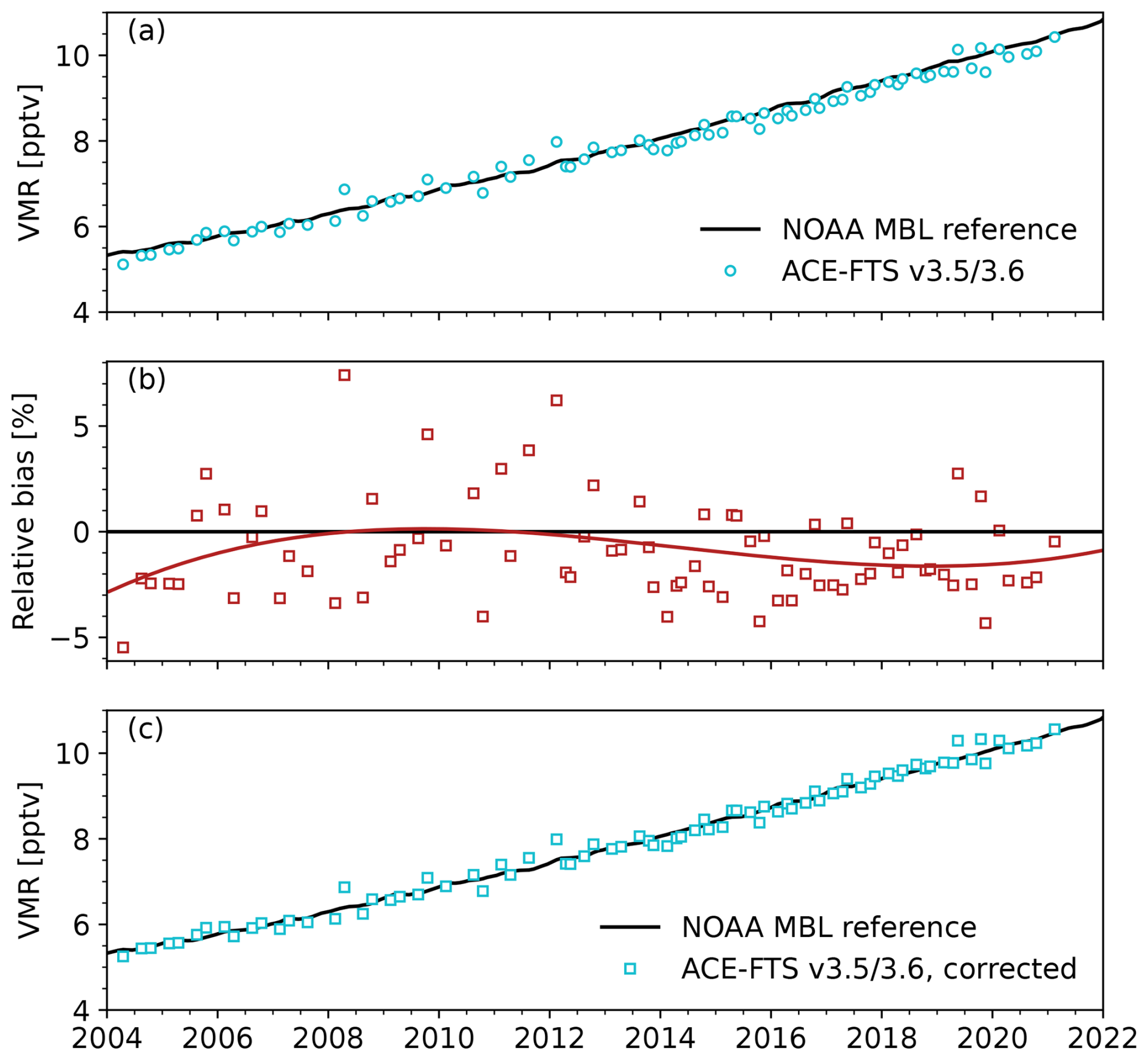
Figure 3 (a) Monthly tropical tropospheric SF₆ time series from the NOAA MBL reference data (black line) and ACE-FTS (blue circles; see text for definition of tropics and troposphere). (b) Relative difference between the monthly ACE-FTS SF₆ values and the reference time series (red squares), with a cubic fit to the data (red line). (c) Same as panel (a) but with the surface correction applied to the ACE-FTS values (blue squares).

A similar method was applied to the MIPAS dataset. The correction was linear, and there was a mean positive bias of 1.8 %, which was removed by dividing the VMR in each bin by 1.018.

4.3 Age-of-air calculation

If an air parcel were not subject to any mixing, then the amount of SF₆ within it could simply be matched to the reference time series and the time lag would correspond to the parcel's exact age. However, this is never a practical assumption, so it is necessary to consider mixing and treat measured (and modelled) air parcels with an age spectrum. The age spectrum was approximated using an inverse Gaussian function (Waugh and Hall, 2002):

$$\begin{array}{}\text{(1)}& G(\mathrm{\Gamma },\mathrm{\Delta },t)={\displaystyle \frac{{\mathrm{\Gamma }}^{\mathrm{3}/\mathrm{2}}}{\mathrm{2}\mathrm{\Delta }\sqrt{\mathit{\pi }{t}^{\mathrm{3}}}}}\exp \left({\displaystyle \frac{-{\mathrm{\Gamma }}^{\mathrm{3}}(t/\mathrm{\Gamma }-\mathrm{1}{)}^{\mathrm{2}}}{\mathrm{4}{\mathrm{\Delta }}^{\mathrm{2}}t}}\right),\end{array}$$

where t is the transit time, Γ is the mean age and Δ is the width of the distribution. Prior studies assumed that the “ratio of moments”, $w={\mathrm{\Delta }}^{\mathrm{2}}/\mathrm{\Gamma }$, was a constant value of 0.7 years as in Waugh and Hall (2002). For this study, the ratio of moments for each latitude and altitude was taken from a model study based on a Chemical Lagrangian Model of the Stratosphere (CLaMS) run (Ploeger et al., 2021) that used winds from ERA-Interim and an exponential fit correction to fit the tail of the spectrum. This ratio of moments is assumed to be constant in time, which is consistent with the use of an inverse Gaussian for the age spectrum. For more details on this approach, see Garny et al. (2024b). Generally, this parameter is the source of considerable uncertainty as w values are much larger for ERA5 than for ERA-Interim, for example. ERA-Interim was chosen because of its close agreement with the observed circulation based on age of air (Linz et al., 2017). The w value varies from about 0.5 to 1.5 years, with the highest values being found in the extratropical lower stratosphere.

Given that each air parcel has an age distribution rather than one single age, the goal of this calculation is to find the mean of the age spectrum for each parcel (i.e., bin). This requires determining which age spectrum, that is, which Γ value, would yield the bin's mean SF₆ VMR (denoted [SF₆]_measured, following the formalism in Stiller et al., 2012). Since it is not analytically possible to determine the age spectrum based on [SF₆]_measured directly, the inverse problem must be solved instead. That is, given a mean age Γ and a distribution width Δ, the goal is to find the stratospheric entry time and the corresponding tropospheric SF₆ value. This is essentially the same as treating the age spectrum as a probability density function to find an expectation value for [SF₆]_measured. Specifically, the following integral is evaluated:

$$\begin{array}{}\text{(2)}& [{\mathrm{SF}}_{\mathrm{6}}{]}_{\mathrm{measured}}=\underset{\mathrm{0}}{\overset{\mathrm{\infty }}{\int }}\stackrel{\mathrm{̃}}{G}(\mathrm{\Gamma },\mathrm{\Delta },t\left)\right[{\mathrm{SF}}_{\mathrm{6}}{]}_{\mathrm{trop}}(t_{\mathrm{meas}}-t)\mathrm{d}t,\end{array}$$

where $\stackrel{\mathrm{̃}}{G}$ is the normalized age spectrum, t is the transport time, and t_meas is the time of the stratospheric measurement. [SF₆]_trop(t), the tropospheric reference time series (see Sect. 4.1), is evaluated at t_meas−t because the stratospheric SF₆ VMR should correspond to the tropospheric value from t years before the measurement was taken.

The inverse problem is then solved iteratively. The first guess Γ₀ is taken to be the time lag between a stratospheric SF₆ measurement and the time at which that SF₆ value was found in the troposphere (t_trop,0) according to the reference time series. Γ₀ is then used in Eq. (2) along with the distribution width (using ${\mathrm{\Delta }}_{\mathrm{0}}={\sqrt{w\mathrm{\Gamma }}}_{\mathrm{0}}$) for the air parcel's latitude and altitude to obtain the expected stratospheric SF₆ value, denoted hereafter by [SF₆]_modelled. A new guess for the tropospheric time (t_trop,new) is then calculated using Newton's method:

$$\begin{array}{}\text{(3)}& t_{\mathrm{trop},\mathrm{new}}=t_{\mathrm{trop},\mathrm{0}}+{\displaystyle \frac{[{\mathrm{SF}}_{\mathrm{6}}{]}_{\mathrm{measured}}-[{\mathrm{SF}}_{\mathrm{6}}{]}_{\mathrm{modelled}}}{\mathrm{d}\left[{\mathrm{SF}}_{\mathrm{6}}{]}_{\mathrm{trop}}\right(t_{\mathrm{trop},\mathrm{0}})/\mathrm{d}t}}.\end{array}$$

The new guess for the age Γ_new is then taken to be $t_{\mathrm{meas}}-t_{\mathrm{trop},\mathrm{new}}$. This process is repeated, using 4Γ_new as the upper bound on the integral with 1000 intervals, until the difference between [SF₆]_modelled and [SF₆]_measured is below 0.01 pptv, which is well below the standard error of the mean SF₆ value in each bin and typically allows convergence within five iterations.

The uncertainty on the age of air in each bin was estimated in two ways. The first was by propagating the standard deviation of the SF₆ VMR through a simplified age-of-air calculation. That is, the upper bound on the age was taken to be the lag time between the average SF₆ VMR plus the standard deviation and the equivalent point on the tropospheric reference curve. The lower bound was estimated the same way but using the SF₆ VMR minus the standard deviation. The “standard deviation of the age of air” was taken to be half of the range between these two bounds. The same calculation was also done using the standard error of the mean SF₆ VMR to determine the “standard error of the mean age of air”. Both of these uncertainties are provided in the data files.

4.4 Mesospheric sink correction

The calculation described above assumes that SF₆ has no chemical sources or sinks in an air parcel observed in the stratosphere. However, some air in the stratosphere has travelled through the mesosphere and therefore been depleted of SF₆. This is especially true at higher altitudes and within the polar vortex. In these regions, SF₆ has a lower VMR for a reason other than older age of air, which the above calculation does not account for. Garny et al. (2024a) have established a correction scheme to address this bias in the “apparent” (i.e., uncorrected) age and determine the “ideal” (i.e., sink-corrected) age. Garny et al. (2024a) showed that the apparent age $\stackrel{\mathrm{̃}}{\mathrm{\Gamma }}$ is approximately related to the ideal age Γ by the following:

$$\begin{array}{}\text{(4)}& \stackrel{\mathrm{̃}}{\mathrm{\Gamma }}=\mathrm{\Gamma }\left(\mathrm{1}+{\displaystyle \frac{F_t\left(t_{\mathrm{meas}}\right)}{{\mathit{\tau }}_{\mathrm{eff}}}}\right),\end{array}$$

where τ_eff is the effective lifetime of stratospheric SF₆, t_meas is the stratospheric measurement time, F_t(t_meas) is the ratio of the reference tropospheric mixing ratio to its time derivative evaluated at t_meas−Γ₀, and Γ₀ is the linearization point for the Taylor expansion of the reference time series [SF₆]_trop(t_meas) (see Garny et al., 2024a, for details). As recommended by Garny et al. (2024a), Γ₀ was set to 4 years, and τ_eff was calculated using τ_eff=αexp(βΓ), where α and β are 5.21×10² and $-\mathrm{3.81}\times {\mathrm{10}}^{-\mathrm{1}}$, respectively. F_t(t) was calculated using the reference time series described in Sect. 4.1, with the time derivative in the denominator taken to be the slope of the tangent line over a 5-year period centred on t_meas.

For each apparent age value at time t_meas,i, that is, the age derived for each bin in the ACE-FTS and MIPAS SF₆ climatologies, F_t(t_meas) was determined for the relevant year, and Eq. (4) was solved numerically to find the ideal age. The uncertainty on sink-corrected age of air was estimated by applying the sink correction scheme to the age plus the estimated uncertainty and to the age minus the estimated uncertainty and using half the range of these two values. This was done for both the standard deviation and the standard error of the mean. It is important to note that the sink correction only depends explicitly on time and not on altitude or latitude. However, there is an implicit altitude and latitude dependence since the ideal age depends on the apparent age, and the apparent age changes with altitude and latitude. This is not a comprehensive treatment of the spatial dependence, as 2-year-old air in the tropics has less mesospheric influence than 2-year-old air in the poles, for example. In addition, the sink correction has so far only been derived from model data, and there is uncertainty in how well the model simulates the sink. In particular, the sink correction cannot completely remove the bias for air older than about 5 years (Garny et al., 2024a).

5 Results and discussion

The multi-year zonal mean apparent age of air derived from ACE-FTS (i.e., without the sink correction) is shown in Fig. 4. The annual means from 2004 through 2021 were averaged together so that each year was weighted equally. As expected, age increases with height and with latitude following the flow of the BDC. The apparent age is older in the Southern Hemisphere at high altitudes because the polar vortex is stronger and SF₆-poor air descending from the mesosphere is kept isolated from younger midlatitude air. In the remainder of this section, the ACE-FTS derived age of air is investigated in more detail through an exploration into the effects of the mesospheric sink correction and comparisons with age of air derived from MIPAS and from other observational datasets. Finally, applications of the ACE-FTS derived age-of-air product are demonstrated through a comparison with CMAM39 and an exploration of the long-term trend in age of air.

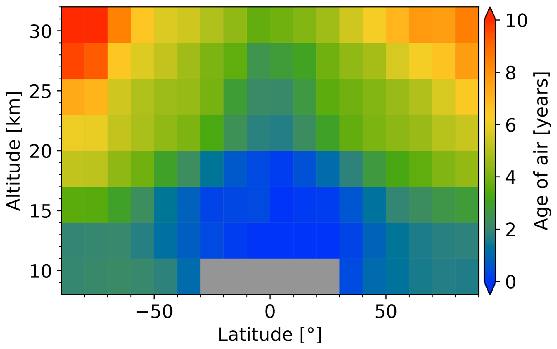
Figure 4 Multi-year zonal mean apparent age of air based on the ACE-FTS SF₆ dataset (February 2004–February 2021).

5.1 Effect of the mesospheric sink correction

This section explores the effect of the mesospheric sink correction described in Sect. 4.4 on age of air derived from both ACE-FTS and MIPAS. Figure 5 shows the zonal mean ages derived from ACE-FTS for each season with (middle row) and without (top row) the sink correction, alongside the difference (bottom row). The mean WMO tropopause height, averaged into 5° latitude bins, is also shown. The absolute difference uses the uncorrected age as the reference, so negative values correspond to a decrease in age as a result of the sink correction. The influence of mesospheric air can be seen throughout the seasons at higher altitudes and latitudes. Air appears oldest in the upper stratosphere at high southern latitudes during austral winter and spring where subsidence within the polar vortex is strongest. A similar ageing effect can be seen in the northern polar vortex during boreal winter, but to a lesser extent due to increased mixing with the midlatitudes. The absolute differences between the uncorrected and corrected zonal means are below 2 years throughout most of the stratosphere but are quite large in these polar regions with high subsidence. In the southern polar vortex, the sink correction decreases the derived age by up to 6 years.

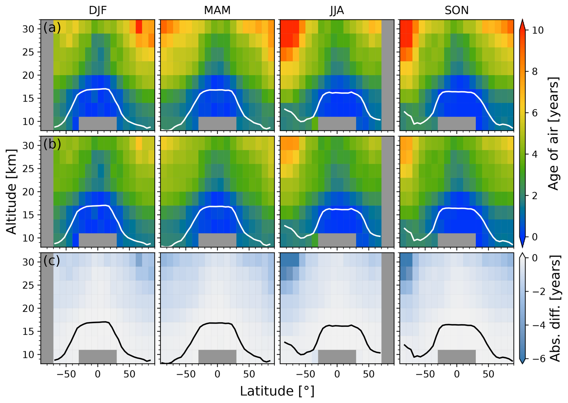
Figure 5 (a) Multi-year zonal mean age of air from the full ACE-FTS v3.5/3.6 dataset (February 2004–February 2021). Each column represents one season. (b) Same as row (a) but with the sink correction applied. (c) Absolute differences between the sink-corrected and uncorrected ACE-FTS ages (corrected minus uncorrected). The mean WMO tropopause height is shown in white in rows (a) and (b) and in black in row (c).

The sink correction has a similar effect on MIPAS ages, as shown in Fig. 6. Note that here the full MIPAS dataset has been used. Similarly to ACE-FTS, the effect of the sink correction is amplified at high latitudes. The correction has a larger effect on MIPAS than on ACE-FTS at midlatitudes between 20 and 30 km. This is to be expected given that the MIPAS ages in these regions are older than those from ACE-FTS, particularly above 25 km, where the sink correction decreases the age by up to 3 years even in the lower midlatitudes.

Figure 6 Same as Fig. 5 but for the full MIPAS V5R dataset (2005–2012).

For both datasets, even with the sink correction, the air at high latitudes and altitudes is significantly older than in other regions. This difference could be at least partially explained by the fact that the sink correction is known to undercorrect for air older than about 5 years (Garny et al., 2024a). Further validation of the SF₆ sink correction beyond the model-based analysis of Garny et al. (2024a) would require the comparison against age-of-air estimates from other clock tracers, which have not been available so far, and so this is left for future studies. However, one such comparison has been done for vortex air from the SOLVE campaign for the Northern Hemisphere, and CO₂ ages reached about 6 years between 25–32 km (Ray et al., 2017). This is only from one flight, however, and is not necessarily representative.

5.2 Comparison with MIPAS

For the comparisons shown here, only coincident ACE-FTS and MIPAS measurements were considered, so the number of measurements included in each bin is reduced compared to when the full datasets are used.

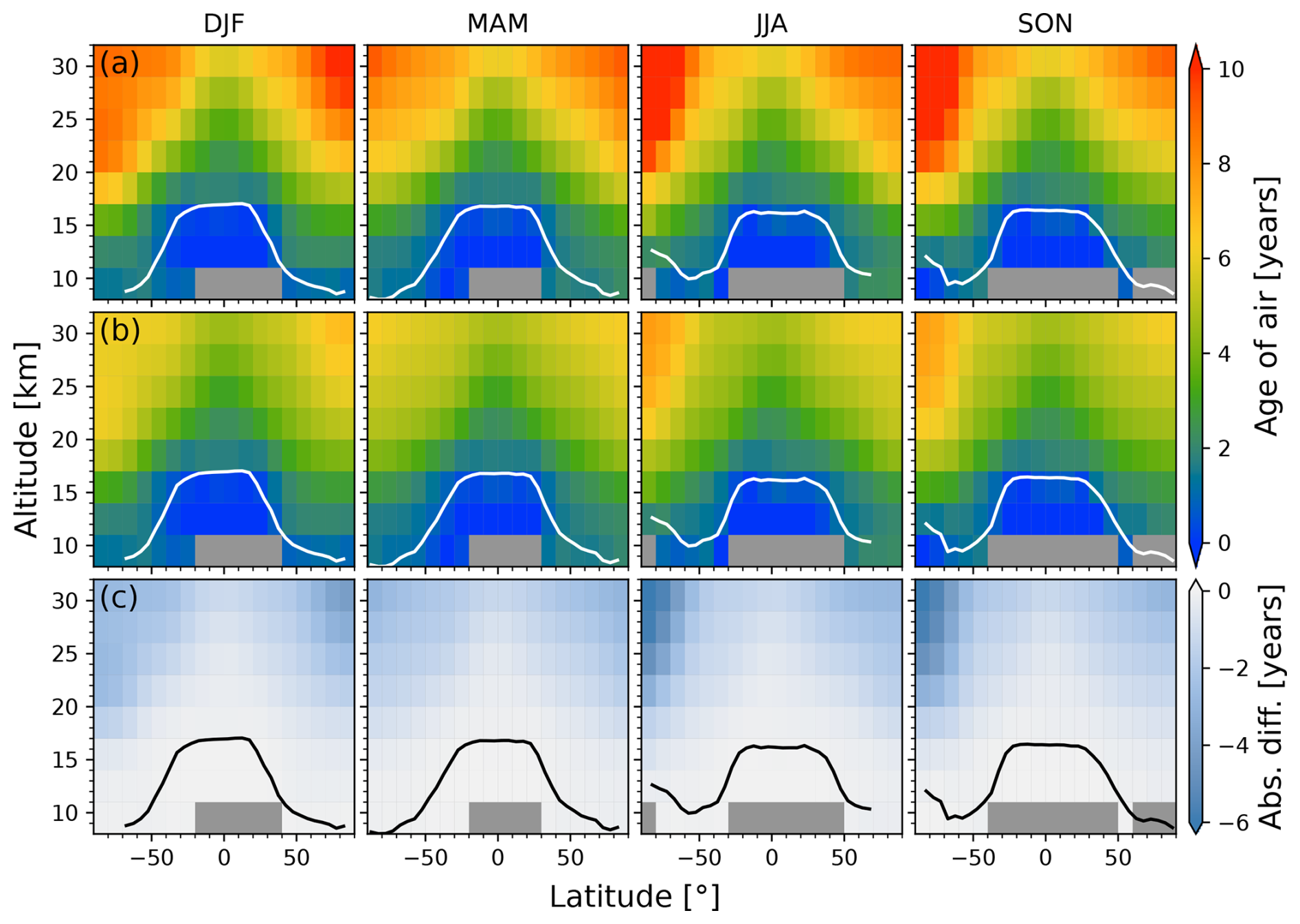
Figure 7 shows the multi-year seasonal zonal mean uncorrected age of air for ACE-FTS (top row) and MIPAS (middle row), as well as the differences between them (bottom row). The general patterns in the zonal means are the same. Age of air increases with both height and latitude and is high inside the Antarctic polar vortex, partially due to the influence of mesospheric air (only relevant for uncorrected age) and partially due to the longer transit times to these locations. The agreement is also good, within 6 months, in the middle to high latitudes at below about 20 km, which is an important region when investigating the BDC. This is the endpoint of the shallow branch of the BDC, so if the satellite-based ages are consistent here, then they can be used to investigate changes in the circulation with more certainty. MIPAS shows older air than ACE-FTS almost everywhere except near the tropopause and above 29 km poleward of 60° S in March–April–May (MAM) and June–July–August (JJA). This is not surprising given that MIPAS SF₆ VMRs are smaller than those from ACE-FTS above 20 km, particularly outside the polar vortex, with a stronger vertical gradient such that the inter-instrument difference becomes larger with altitude (see Sect. 3). Below 20 km, the ACE-FTS and MIPAS ages are generally within a year of each other except in the tropics from 17–20 km, where MIPAS air is up to about 2 years older due to the reduced measured SF₆ values in this region (see Fig. 1).

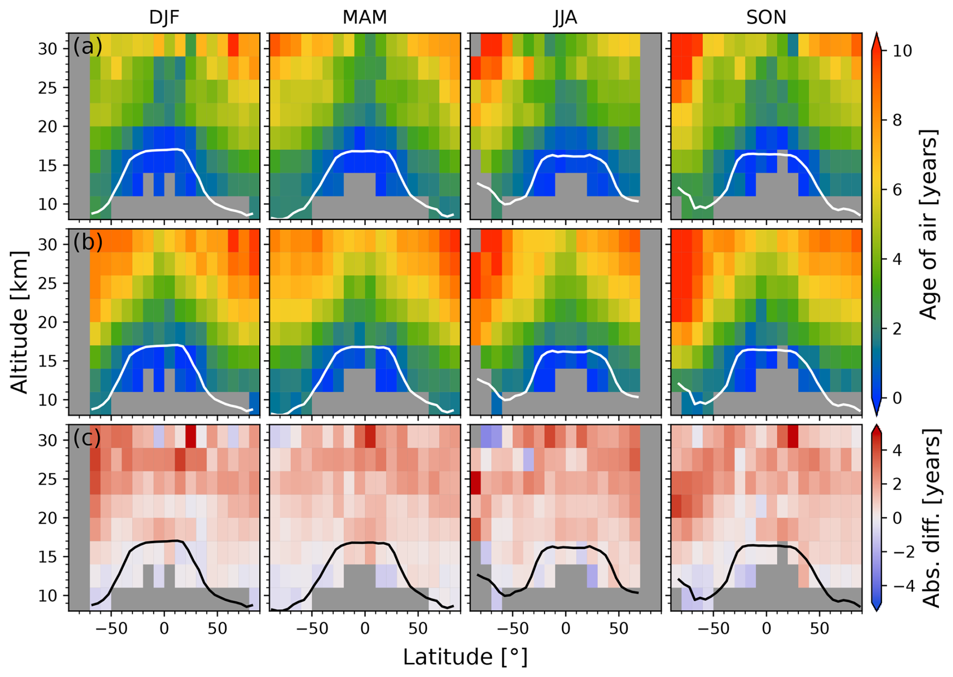
Figure 7 Multi-year (2005–2012) zonal mean uncorrected age of air derived from coincident (a) ACE-FTS and (b) MIPAS measurements. Row (c) shows the absolute differences (MIPAS − ACE-FTS). Each column corresponds to one season. The mean WMO tropopause height is shown in white in rows (a) and (b) and in black in row (c).

The comparisons between the sink-corrected ACE-FTS and MIPAS ages are shown in Fig. 8. The main conclusions are similar, though the difference in age at higher altitudes is reduced because of MIPAS ages being more affected by the sink correction than those from ACE-FTS. This is simply because the sink correction affects older ages more than younger ages, and MIPAS ages are older due to having smaller SF₆ VMRs compared to ACE-FTS. The two datasets have better agreement with the sink correction having been applied, especially in the middle to high latitudes above 20 km where the difference between the ages decreased from up to 6 years to typically less than 4 years. The tropics are still quite different above 25 km, where the difference is still about 3–4 years; however, this is not surprising as the sink correction does not have as much of an effect on younger air.

Figure 8 Same as Fig. 7 but with the sink correction applied to both datasets.

The ACE-FTS and MIPAS ages show similar patterns, though the MIPAS ages are up to 3 years (more than 50 %) older at higher altitudes and latitudes with the mesospheric sink correction applied. It is clear that the difference in vertical gradient of measured SF₆ between the two instruments impacts the derived age of air. Future studies should include comparisons to datasets with ages derived using other clock tracers where ACE-FTS and MIPAS have better agreement.

5.3 In situ comparisons

In situ measurements are a particularly useful reference for comparison. Here, ages calculated from several balloon and aircraft campaigns from 1993 to 2017 (discussed in Sect. 1) are compared with the ACE-FTS age-of-air dataset. Both the sink-corrected and uncorrected ACE-FTS ages are included in these comparisons since the in situ ages use both SF₆ and other tracers such as CO₂. The uncorrected ACE-FTS ages are compared with in situ ages based on SF₆, which are also uncorrected, while the sink-corrected ACE-FTS ages are compared with those from other tracers with no or very small mesospheric sinks.

Table 1 summarizes the details of the aircraft and balloon campaigns used for comparison. For each aircraft flight, age of air has been derived from SF₆ along with several fluorine-containing compounds (see references in Table 1 for age calculation used for each flight). As such, two types of age are shown in Fig. 9: that derived from SF₆ (grey triangles, top row) and the averaged age derived from all measured clock tracers (black circles, bottom row). The uncorrected ACE-FTS ages are shown in the top row, while the sink-corrected ages are shown in the bottom row. The nearest bin (or in some cases, bins) in space and time from the ACE-FTS age dataset was (were) selected for comparison, and each bin is shown as one point, with error bars representing 1 standard deviation of the age of air (as described above). Where multiple bins with the same altitude were used, the points are separated vertically on the plot for better visibility, but the bins are all centred on the same altitude (9.5, 12.5, 15.5, or 18.5 km).

Leedham Elvidge et al. (2018)Leedham Elvidge et al. (2018)Leedham Elvidge et al. (2018)Adcock et al. (2021)Adcock et al. (2021)Harnisch et al. (1996)Harnisch et al. (1996)Andrews et al. (2001)Andrews et al. (2001)Andrews et al. (2001)

Table 1 Overview of the in situ datasets used for comparison with the ACE-FTS age-of-air product. The table is divided into campaigns that occurred during the ACE-FTS mission (top) and those that occurred prior to the mission (bottom). The former are from aircraft campaigns while the latter are balloon campaigns.

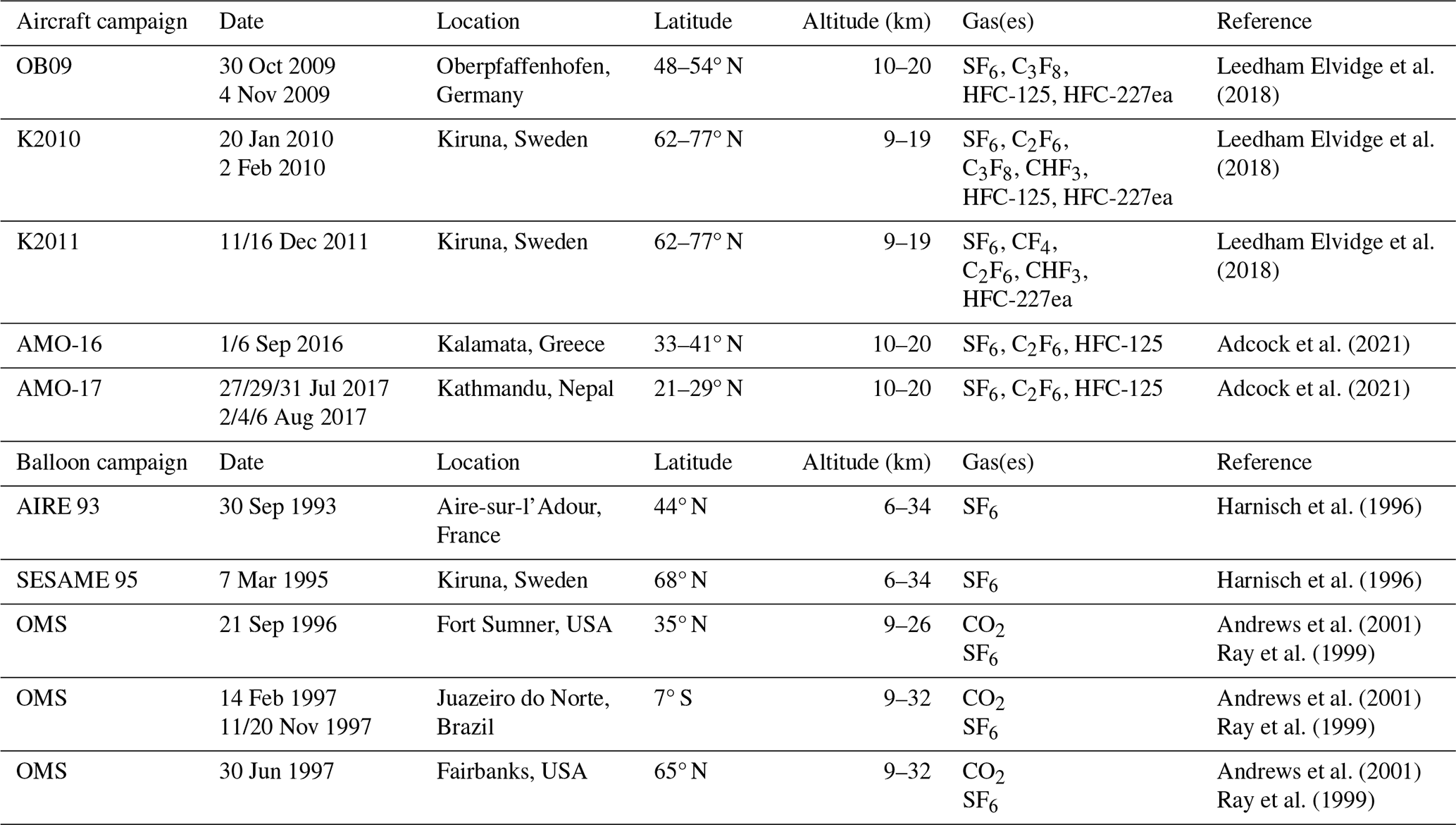
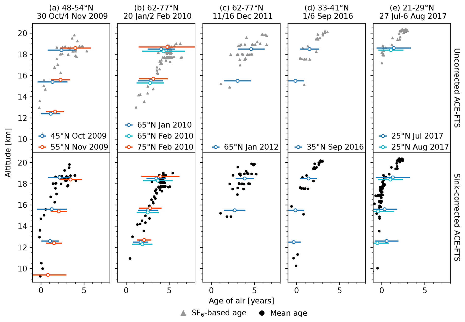
Figure 9 Comparisons between the ACE-FTS age-of-air dataset and ages based on aircraft in situ measurements taken during the ACE-FTS mission. Each column corresponds to one campaign: (a) OB09, (b) K2010, (c) K2011, (d) AMO-16, and (e) AMO-17. See Table 1 for further details. Black dots: mean age of air based on all clock tracers included in the campaign. Grey triangles: age of air based on SF₆. Open coloured circles: mean age of air for one bin in the ACE-FTS dataset (top: uncorrected; bottom: sink-corrected). Points for ACE-FTS bins centred on the same altitude are separated vertically for visibility. Error bars show the standard deviation of the age in each bin.

In nearly all cases, the ACE-FTS ages agree with the aircraft data (i.e., the aircraft data are within 1 standard deviation of the satellite data). Exceptions include the two ACE-FTS bins at 12.5 km in October and November 2009 for both the uncorrected and the sink-corrected ages. The age in both latitude bins is 1–2 years older (more than 1 standard deviation) than the nearest aircraft age at 13 km. This is related to the unrealistic decrease in ACE-FTS SF₆ below about 14 km, which biases the derived age older. In the case of the November 2009 bin centred on 55° N at 15.5 km, the ACE-FTS age is also more than 1 standard deviation from the nearest aircraft age. This can likely be explained by sampling differences; the aircraft age is based on a measurement taken at 48° N, and the ACE-FTS bin does not include this latitude. Conversely, the ACE-FTS age in the bin centred on 45° N does include 48° N and is consistent with the aircraft age. Sampling differences can also explain why a few aircraft ages also fall outside 1 standard deviation from the ACE-FTS ages in December 2011. The ACE-FTS bin is from January 2012, while the aircraft data were taken in mid-December 2011. There are no cases where the sink-corrected ages are consistent while the uncorrected ages are not, and vice versa. This was expected, since the uncorrected ages were only compared with similarly uncorrected age derived from SF₆, and the sink-corrected ages were only compared with ages based on other clock tracers.

The ACE-FTS ages were also compared with the age derived from five balloon campaigns prior to the beginning of the satellite mission. Here, only the time of year was considered (as opposed to the exact month and year), so a balloon campaign from September 1993, for example, was compared with all Septembers of the ACE-FTS mission averaged together. This introduced a temporal bias, especially considering the fact that age of air is potentially changing over time. As such, these comparisons, which are shown in Fig. 10, are more useful for looking at the vertical structure and tentatively comparing age of air between two time periods. For these comparisons, the sink-corrected ACE-FTS ages are shown on the same plots as the uncorrected ages, but as filled markers rather than open markers. The error bars represent the standard deviation of the mean age of air in the bins that were averaged together across all years. The sink-corrected ages are best compared to the in situ ages derived from CO₂, so they are not included in comparisons with flights without CO₂ ages (September 1993 and March 1995). Two times of year were considered for the comparison with the 1997 campaign in Brazil because it included flights in both February and November. As before, the two ACE-FTS bins are vertically separated for visibility but are still centred on the same altitude.

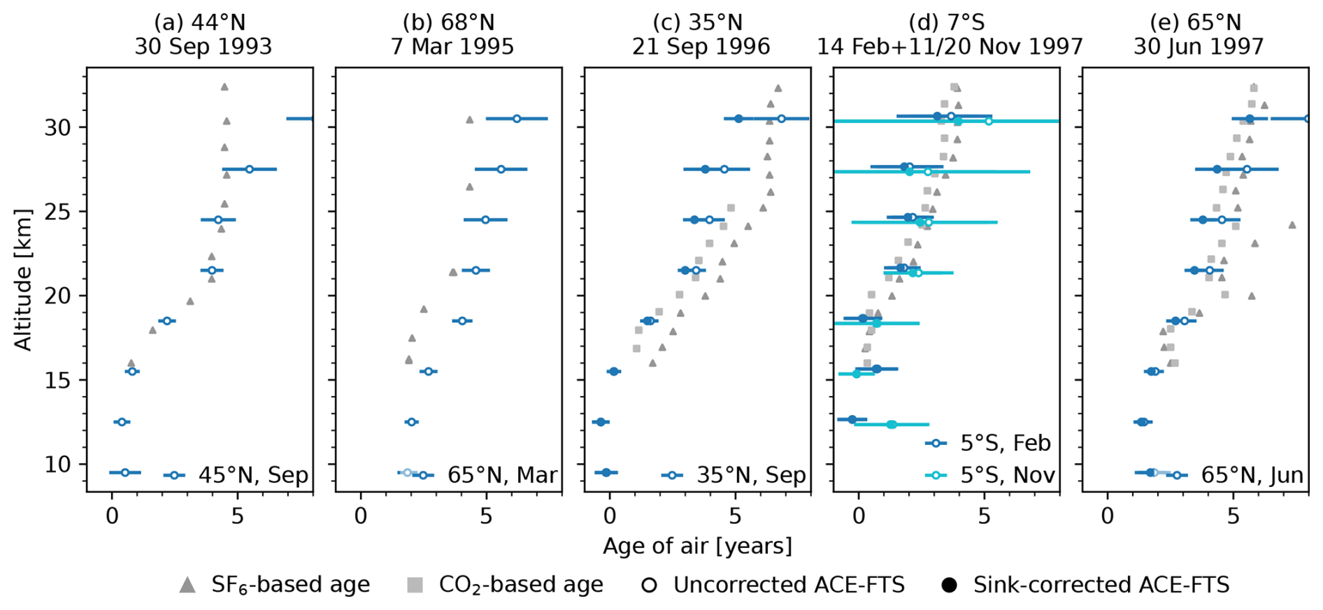
Figure 10 Comparisons between the ACE-FTS age-of-air dataset and ages based on balloon in situ measurements taken prior to the ACE-FTS mission. Each panel corresponds to one in situ campaign: (a) AIRE 93, (b) SESAME 95, and (c–e) OMS. See Table 1 for further details. Grey triangles: age of air based on SF₆. Grey squares: mean age of air based on all clock tracers included in the campaign. Open coloured circles: average uncorrected age of air for a set of bins (e.g., all Septembers at 45°N) in the ACE-FTS dataset. Filled coloured circles: average sink-corrected age of air for a set of bins in the ACE-FTS dataset. Points for ACE-FTS averages centred on the same altitude are separated vertically for visibility. Error bars correspond to 1 standard deviation of the mean ages from the bins that were averaged together.

The agreement between the ACE-FTS and balloon ages varies by location. A common feature in the in situ ages, visible in the profiles from AIRE 93 (September 1993), SESAME 95 (March 1995), and OMS 1996 (September 1996), is a constant age above about 20–25 km. The ACE-FTS profiles do not have this feature. Aside from this difference, the ACE-FTS ages agree with the AIRE 93 (September 1993) ages below 30 km. At 30.5 km, however, the ACE-FTS age is nearly 4 years (100 %) older. The ACE-FTS ages are consistently 1–2 years older than the SESAME 95 (March 1995) ages. This is consistent with a change to the northern deep branch of the BDC between 1995 and the mid-2000s but could also be due to interannual variability. For the OMS flight over the southern USA (September 1996), the uncorrected ages are consistently 1–2 years younger than the in situ ages derived from SF₆, except at 30.5 km. The sink-corrected ages agree with the in situ CO₂ ages below 20 km but are up to one year younger above this point. The differences at lower levels (below about 25 km) could be consistent with an acceleration of the shallow branch of the BDC. The ACE-FTS ages are mostly consistent with those derived from measurements over Brazil (February and November 1997), though the variability is high. The uncorrected ACE-FTS ages mostly agree with in situ SF₆ ages from the flight over Alaska (June 1997) within a few percent. The SF₆ in situ ages are variable, and Andrews et al. (2001) attribute this to remnants of the polar vortex containing mesospheric air. The sink-corrected ACE-FTS ages agree with the CO₂ in situ ages within a few percent everywhere except 20–25 km, where the ACE-FTS ages are slightly (up to about 1 year) younger. This is also consistent with a BDC acceleration, but the difference is small relative to that seen for SESAME 95 and OMS 1996, and the presence of the polar vortex significantly complicates the comparison. Overall, the significant variability in age over time inhibits trend interpretation from these limited in situ comparisons.

The zonal mean ages derived from the full ACE-FTS and MIPAS datasets were also compared with a latitudinal cross-section of ages based on aircraft measurements of SF₆ and CO₂ taken between 1992 and 1997 (Boering et al., 1996; Elkins et al., 1996), shown in Fig. 11. It is important to note that the in situ ages derived from SF₆ have not been sink-corrected, so they are equivalent to the uncorrected ages from ACE-FTS and MIPAS (solid lines). As before, the sink-corrected ACE-FTS and MIPAS ages (dashed lines) should be more similar to the in situ ages derived from CO₂. The error bars on the ages based on CO₂ indicate 1σ uncertainty. The in situ measurements were all taken between 19.5 and 20.5 km, so the ACE-FTS and MIPAS ages for this comparison were calculated using the SF₆ climatologies with the 19–21 km altitude bin. Additionally, these ages were calculated for 5° latitude bins to increase the resolution of the latitudinal cross-section.

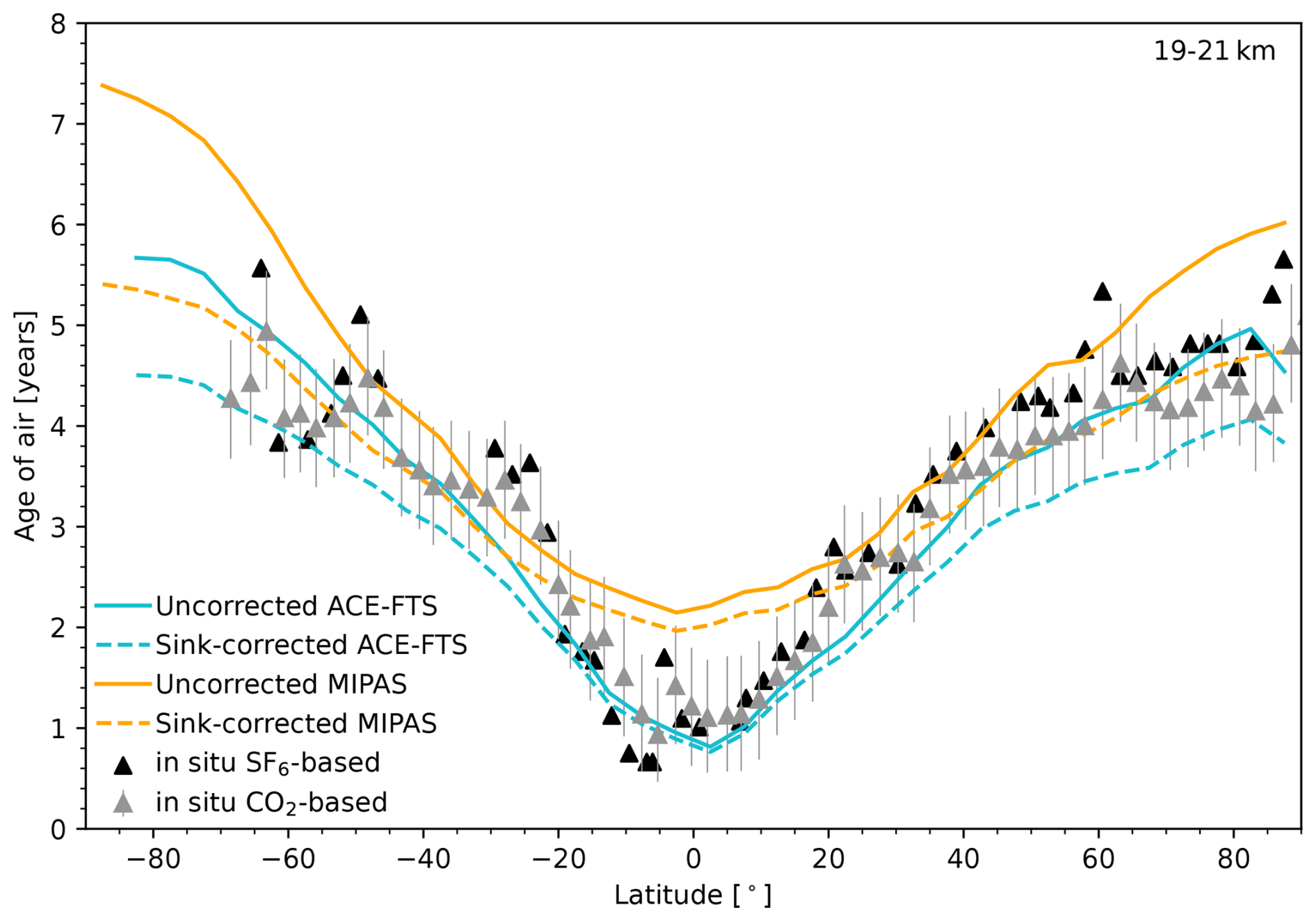
Figure 11 Age of air as a function of latitude, based on in situ measurements of SF₆ (black triangles), in situ measurements of CO₂ (grey triangles with 1σ error bars), ACE-FTS (blue lines), and MIPAS (orange lines). The dashed lines represent the sink-corrected ages from ACE-FTS and MIPAS. The in situ measurements are aircraft measurements taken between 1992 and 1997 at 19–21 km. The ACE-FTS and MIPAS ages are based on the full datasets, with all measurements taken between 19 and 21 km averaged into 5° latitude bins.

Figure 11 shows that uncorrected ACE-FTS ages agree better with the in situ ages derived from SF₆ than the uncorrected MIPAS ages in the tropics and high latitudes, but they are slightly too young (by less than 1 year) in the midlatitudes. With the sink correction applied, ACE-FTS ages are still younger than those from MIPAS and the aircraft data, but they are still mostly consistent with the ages based on CO₂, except between about 20 and 40° S and near 60° in both hemispheres. It is possible that the differences between the aircraft and ACE-FTS altitude and latitude sampling result in ACE-FTS ages being younger. In particular, the aircraft data could show more distinct mixing barriers than are visible in the satellite data, which average over more time and area. The difference could also be due to the time periods covered by the two datasets (2004–2021 for ACE-FTS vs. 1993–1997 for the aircraft data). If so, this result would indicate that age of air is decreasing over time in the midlatitudes, which could be consistent with an acceleration of the shallow branch of the BDC. A conclusion cannot yet be drawn regarding whether the apparent change in age of air over time is due to biases between the different SF₆ measurements or an actual decrease, so further analysis is required.

5.4 Comparison with CMAM39

CMAM39 is a chemistry–climate model based on the extended version of the Canadian Centre for Climate Modelling and Analysis third-generation Atmospheric General Circulation Model (Scinocca et al., 2008) and includes an extensive description of stratospheric chemistry (de Grandpré et al., 2000; Jonsson et al., 2004). The meteorological fields (temperature and horizontal winds) in the specified dynamics version are “nudged” toward ERA-Interim reanalysis (Dee et al., 2011) up to 1 hPa with a relaxation time constant of 24 h. The nudging constrains the large-scale dynamics to follow the reanalysis, allowing for a direct comparison between the model and measurements, though nudging has also been shown to modify certain aspects of the BDC as compared with a free-running simulation (Chrysanthou et al., 2019). The modelled age of air is based on an idealized SF₆ tracer, meaning that it is not subject to the mesospheric sink. Therefore, the sink-corrected ACE-FTS ages were used for this comparison, which spans the 2004–2018 period where ACE-FTS and CMAM39 overlap. To account for sampling differences, CMAM39 has been subsampled onto the ACE-FTS times and locations using an updated version of the advanced method described in Kolonjari et al. (2018). Here, the modelled values were also linearly interpolated in time instead of using a nearest-neighbour approach.

The comparisons for each season are shown in Fig. 12, where the ACE-FTS ages are shown in the top row, the CMAM39 ages are shown in the middle row, and the differences (CMAM39 − ACE-FTS) are shown in the bottom row. ACE-FTS and CMAM39 agree within 6 months below about 24 km, and it is noteworthy that the modelled ages are mostly younger than the observed ages. Kolonjari et al. (2018) found evidence that the BDC in CMAM30, the predecessor to CMAM39 that was also nudged to ERA-Interim, was too fast, which would result in younger stratospheric air and be consistent with these results. It was also found that at pressures less than 150 hPa, the age in CMAM30 was up to 1 year older than the age in the free-running version, suggesting that nudging affects the strength of the BDC and tracer transport. The largest differences between the ACE-FTS and CMAM39 ages are at high altitudes and latitudes, particularly in the winter and spring, where ACE-FTS air is 3 years older in the Southern Hemisphere. This is not necessarily entirely due to an issue in the model; ACE-FTS ages were also shown to be older than in situ ages at higher altitudes in Fig. 10. It is also possible that the sink correction does not fully account for the high age bias in ages derived from SF₆ measurements. This could be investigated using comparisons between CMAM39 and ages based on other clock tracers.

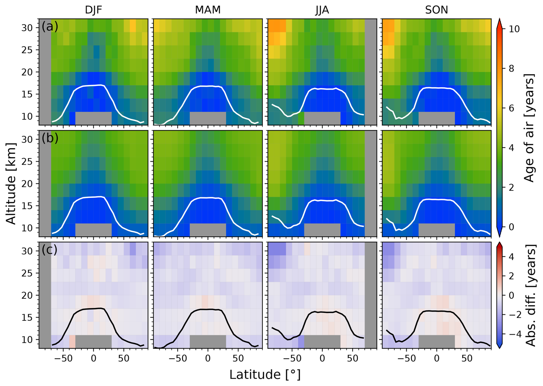
Figure 12 Multi-year (2004–2018) zonal mean age of air derived from (a) ACE-FTS and (b) CMAM39 subsampled to the ACE-FTS measurement grid, with the absolute differences (CMAM39 − ACE-FTS, row c). Each column corresponds to one season. The mean WMO tropopause height is shown in white in rows (a) and (b) and in black in row (c).

5.5 Long-term age-of-air trend

One of the main advantages of the ACE-FTS age-of-air product is the long 17-year time series that version 3.5/3.6 provides. While the MIPAS product has excellent global coverage and density, the mission lasted only about a decade, which makes it difficult to detect a long-term trend in a climate system impacted by multi-year oscillations such as the Quasi-Biennial Oscillation (QBO), the El Niño–Southern Oscillation (ENSO), and the solar cycle. On the other hand, the relative sparsity of ACE-FTS measurements also causes some difficulty in accounting for these oscillations. Each 10° latitude band does not have an ACE-FTS age value for every month as it does for MIPAS, and fitting a time series with gaps is more challenging. Given these limitations, the aim of this work is to investigate whether significant long-term changes in age of air can be detected from ACE-FTS, despite the sparse sampling. The focus is on regions where ACE-FTS has the highest density of successful SF₆ retrievals: the lower stratosphere (14–20 km) between 40 and 70° latitude in each hemisphere. While the profiles at these latitudes do extend higher into the stratosphere, the number of measurements in each bin is reduced at higher altitudes, increasing the standard error of the zonal mean and therefore the uncertainty in the age, which makes trend detection more difficult. Age of air in the lower stratosphere is largely influenced by the shallow branch of the BDC, so changes in this region can indicate whether the shallow branch might be changing. A trend was calculated based on the monthly values for each (10°, 3 km) bin within these two regions.

To calculate the linear trend of each age-of-air time series, a similar approach to the one presented in Stiller et al. (2012) and Haenel et al. (2015) was used. Each sink-corrected time series was fitted using the following function:

$$\begin{array}{}\text{(5)}& \begin{array}{rl}\mathrm{\Gamma }\left(t\right)& =a+bt+c_{\mathrm{1}}{\mathrm{qbo}}_{\mathrm{1}}\left(t\right)+d_{\mathrm{1}}{\mathrm{qbo}}_{\mathrm{2}}\left(t\right)+c_{\mathrm{2}}\mathrm{enso}\left(t\right)\\ & +c_{\mathrm{3}}{\mathrm{sol}}_{\mathrm{1}}\left(t\right)+d_{\mathrm{3}}{\mathrm{sol}}_{\mathrm{2}}\left(t\right)\\ & +\sum _{n=\mathrm{4}}^{\mathrm{5}}\left(c_n\sin {\displaystyle \frac{\mathrm{2}\mathit{\pi }t}{l_n}}+d_n\cos {\displaystyle \frac{\mathrm{2}\mathit{\pi }t}{l_n}}\right),\end{array}\end{array}$$

where t is time in years. The QBO and ENSO variations are included via the proxies qbo₁, qbo₂, and enso. Previous analyses of longer time series of age of air from MERRA2 reanalysis data and of merged observed water vapour (SWOOSH) have also found decadal oscillations, the causes of which are not completely clear (Strahan et al., 2020; Tao et al., 2023). In order to account for these, an oscillation term with a period of about 10 years was included. In the numerical approach, the solar cycle was used for this with proxies sol₁ and sol₂. There is some justification for this given the link between the solar cycle and the velocity of tropical upwelling (Kodera and Shibata, 2006), but this is not sufficient evidence to assume that the decadal oscillation is driven by the solar cycle alone. The final sum term represents the annual and semi-annual cycles, where l₄=1 year and l₅=0.5 years. Other harmonic oscillations were omitted because they resulted in an overfit of the sparse ACE-FTS time series and did not significantly affect the linear term, b. Several versions of this function were tested with different combinations of proxies for the QBO, ENSO, and the decadal variation, and it was determined that including all of them produced the best results. That is, the fit residuals had the least structure when more natural variability was accounted for. To allow for temporal offsets between the QBO time series and the age response at different locations, two orthogonal terms were included. The same holds for the decadal variation. This model differs from that used in Haenel et al. (2015), which used eight different harmonics and did not consider the lower frequency oscillations (ENSO and the decadal variation). The latter two were included here because the length of the time series is nearly doubled and more than one period for each oscillation is covered by the time series. The qbo₁ and qbo₂ vectors are monthly orthogonal normalized Singapore winds at 30 and 50 hPa, respectively (Karlsruhe Institute of Technology, 2025). The ENSO proxy is the Multivariate ENSO Index (NOAA, 2022). The sol₁ term is the monthly adjusted solar flux at 10.7 cm as determined from daily measurements taken in Penticton, Canada, at the Dominion Radio Astrophysical Observatory provided by NOAA (2018) from February to September 2004 and by Space Weather Canada (2022) from October 2004 to February 2021. The orthogonal term, sol₂, is from the same dataset but shifted by 2 years and 9 months, that is, by one-quarter of the solar period of approximately 11 years. As mentioned above, the so-called solar cycle term is included to account for any decadal variation and is not necessarily believed to have solar variability as its cause. Any variation longer than approximately 10 years would not make sense to be fitted to a 17-year time series. With these proxies, the ACE-FTS age-of-air data were fit with Eq. (5) using the method described in von Clarmann et al. (2010) and for irregularly spaced and correlated data. This method uses Gaussian error propagation of the standard error of the monthly zonal mean to calculate the uncertainty on the linear trend, with additional consideration for errors in the regression model using the autocorrelation between the residuals. Details on the latter method can be found in Stiller et al. (2012) and Haenel et al. (2015). Uncertainties due to the sink correction are not considered.

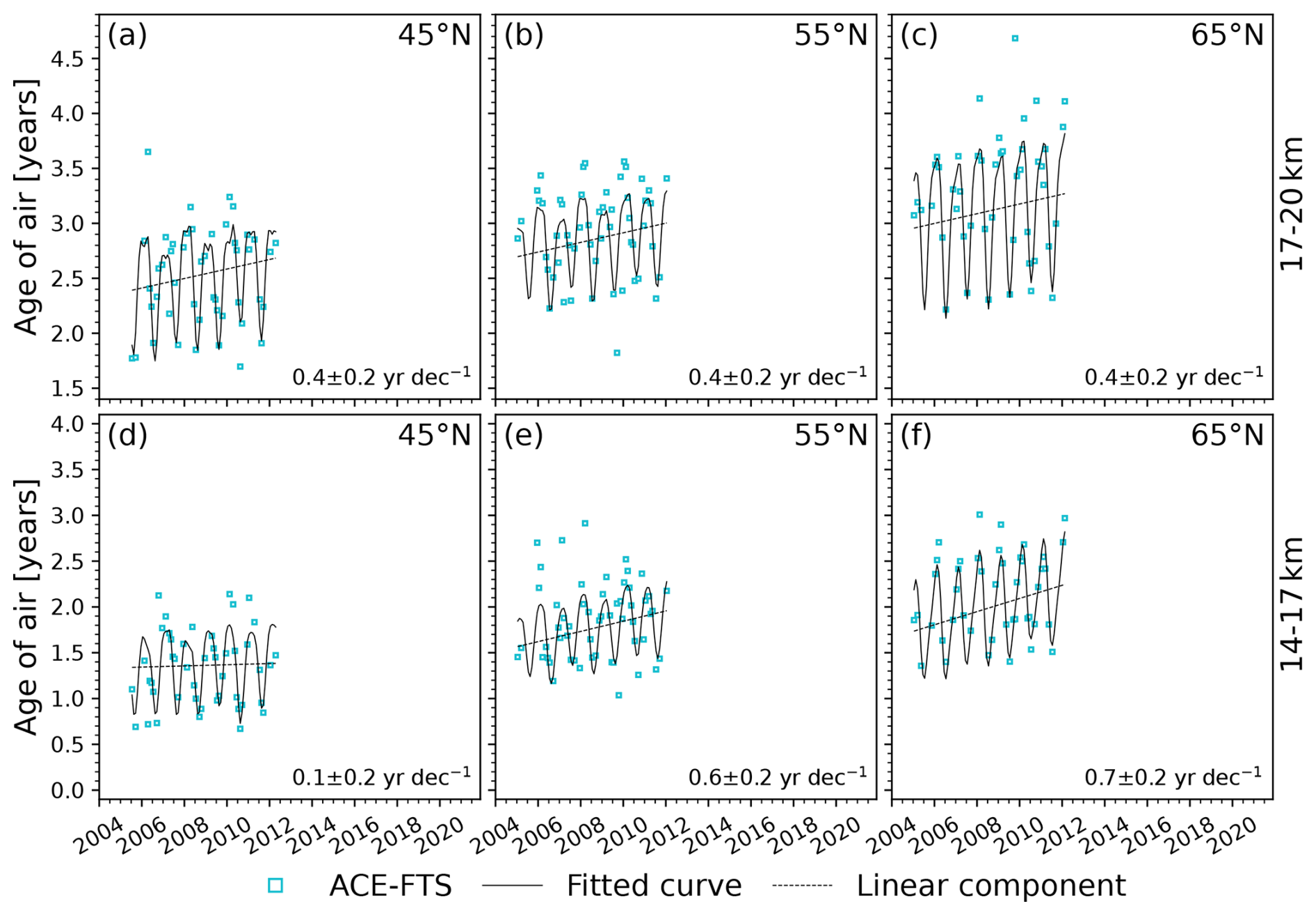
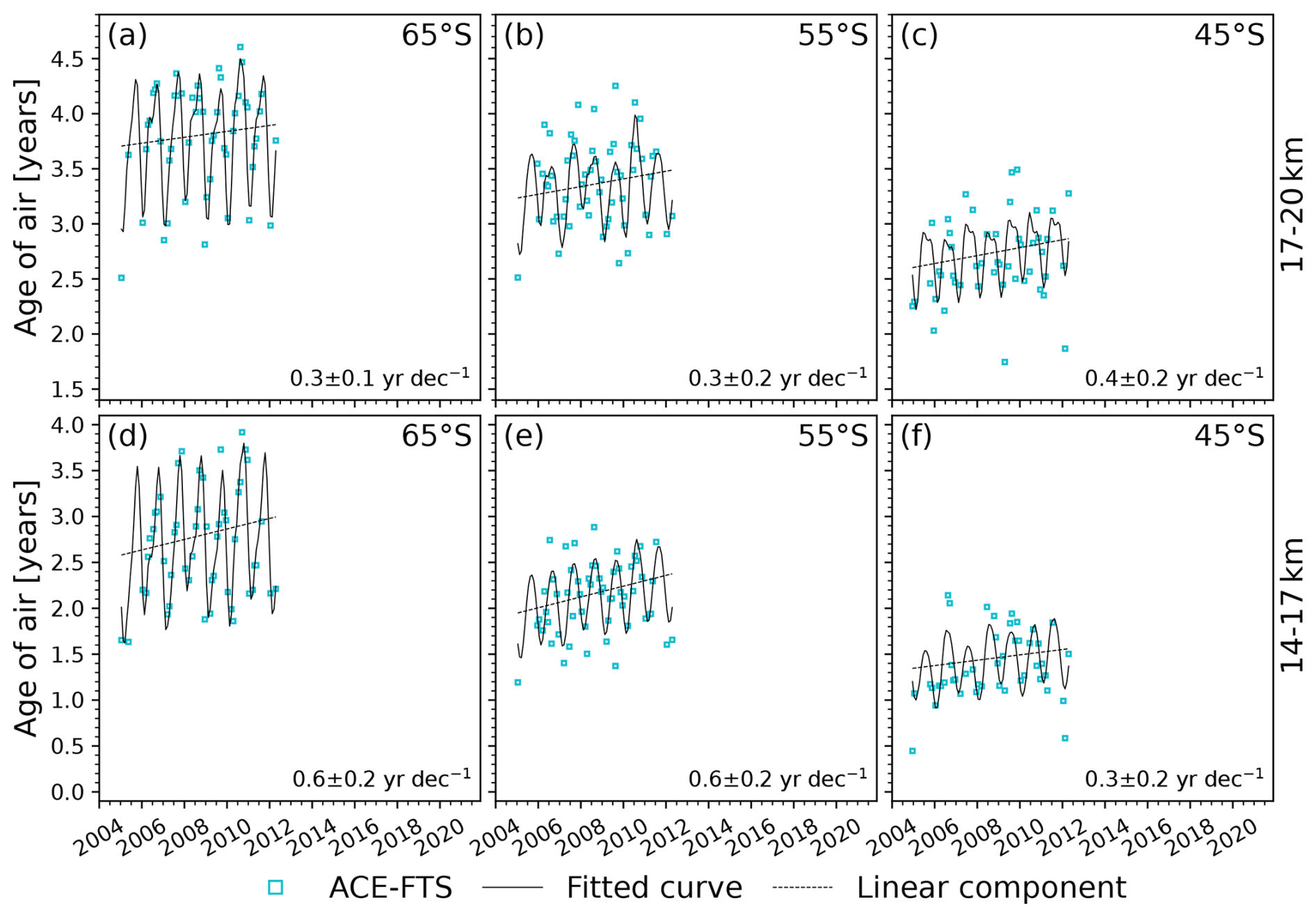
The fitted curves for the Northern and Southern Hemisphere, with the linear component plotted separately (dashed black line), are shown in Figs. 13 and 14, respectively. The linear trend values and their uncertainties are given in the bottom right of each panel. The trend is negative and significant to 2 standard deviations in 4 of the 12 regions: 50–60 and 60–70° S at 17–20 km and 40–50 °N at 14–17 and 17–20 km. Elsewhere, the trend is negative but not statistically significant. For the most part, the fit represents the data fairly well; the residuals did not show noticeable structure. The clearest feature in all bins is the annual cycle, which appears to be mostly well captured though perhaps with a slightly underestimated amplitude at lower latitudes. Similarly to what was observed by Stiller et al. (2012), the amplitude of the seasonal cycle is larger at higher altitudes.

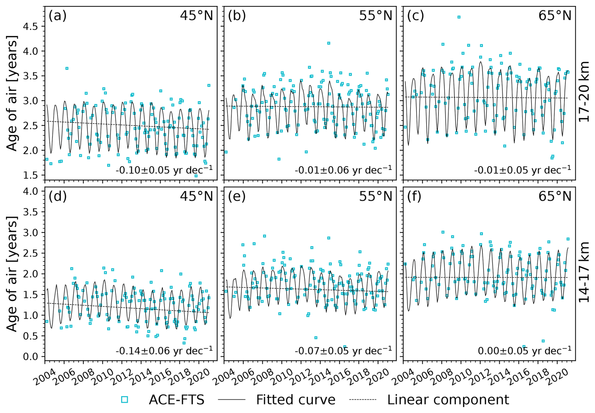
Figure 13 Monthly age of air derived from the ACE-FTS dataset (blue squares), with the full fit described in the text (solid black line) and its linear component (dashed black line). Each panel (a–f) corresponds to one northern hemispheric bin (labelled by the bin centre) in the lower stratosphere, indicated in the figure. The linear trend and corresponding error estimates are shown in the bottom right of each panel.

Figure 14 Same as Fig. 13 but for the Southern Hemisphere.

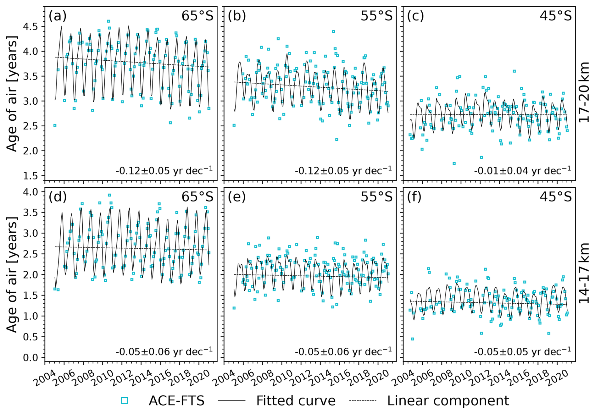
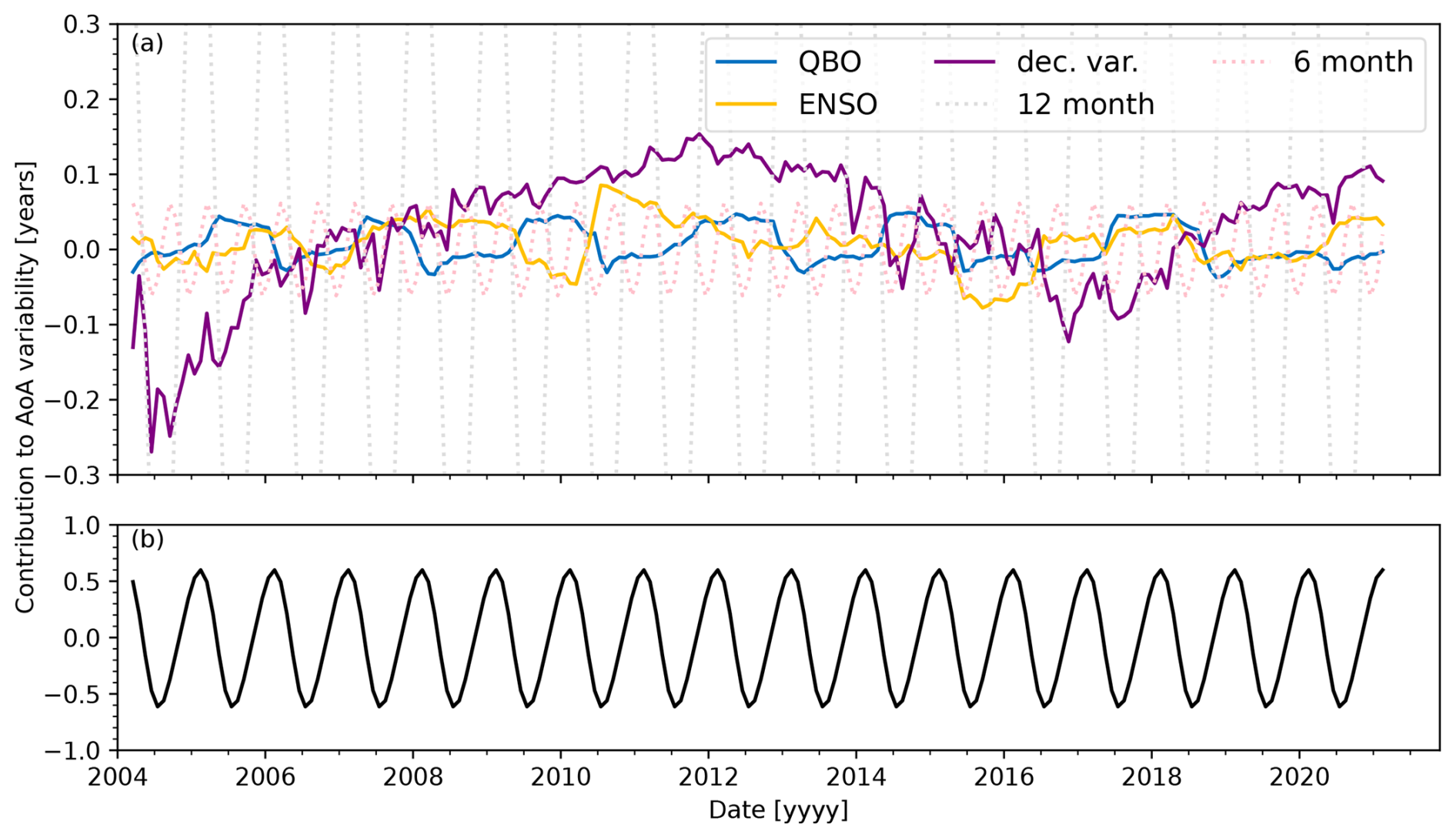
Figure 15 (a) The contribution (in years) of each type of interannual variability to the fitted age of air for 60–70° N, 14–17 km. (b) The total contribution of the 12- and 6-month seasonal cycles.

As an example, the contributions of each type of interannual variability are summarized for 65° N (14–17 km) in Fig. 15. This summary is shown for the other 11 bins in the Supplement. The QBO, ENSO, decadal variation, and semiannual cycles each have similar amplitudes of 1–2 months, with the decadal variation being of particular interest as it is noticeable in the time series shown in Fig. 13 at 55 and 65° N (14–17 km). It appears as a low-frequency oscillation causing an increase in age early in the time series up to around 2010, a decrease until 2016, and an increase afterwards. The solar cycle proxy seems to account for this oscillation well; in every bin, the fit residuals are smaller and have less structure when it is included in the fit. However, even if the time series is fit without the solar cycle term in Eq. (5), the linear trend remains consistent in each bin and is statistically significant in the same regions. Therefore, the sign of the age-of-air trend over the full observation period is independent of the assumption of a solar cycle. These findings signal an acceleration of the shallow branch of the BDC within both hemispheres, if tropical ages are not changing, though the effect is not symmetric. The results in the Northern Hemisphere are in agreement with the results in Ray et al. (2014), which indicated a negative trend in age of air in the northern midlatitudes at 15–20 km.

These trends are also somewhat consistent with what Haenel et al. (2015) found for these regions, which was that the trends in the Northern Hemisphere region were positive but insignificant and most trend values in the Southern Hemisphere were negative but also insignificant except for 40–60° S from approximately 18–20 km. Therefore, there is agreement in the sign of the trend for 50–60°S at 17–20 km (negative trend), 40–70° S at 14–17 km (insignificant trend), and 50–70° N at 14–20 km (insignificant trend). There are several reasons that the trends might not agree in the other regions. As shown in Sect. 5.2, there are discrepancies between the MIPAS and ACE-FTS age-of-air datasets. Furthermore, Haenel et al. (2015) did not apply a sink correction to the MIPAS ages, and a sink correction will change the trend (Loeffel et al., 2022). The regression model used here was also altered through the addition of the decadal variation and ENSO and the removal of several harmonics. Another important difference is that the MIPAS trends were calculated for 2002–2012, while the ACE-FTS trends cover the 2004–2021 time period. To explore the impacts of these differences, the trends in the ACE-FTS age of air were calculated over the period that overlapped with the MIPAS mission, January 2005–April 2012. Since only 8 years of data were included, ENSO and the decadal variation were omitted from the regression, making the fit more similar to that used for MIPAS data in Haenel et al. (2015), though with fewer harmonics as the ACE-FTS data are not as dense. Additionally, the ACE-FTS time series here start in 2005 rather than in 2002 like the time series that were analyzed in Haenel et al. (2015). The resulting fits for the Northern Hemisphere and Southern Hemisphere are shown in Figs. 16 and 17, respectively. In all cases, the fits appear to represent the data well (based on the lack of structure in the residuals), but the linear term is positive and larger in magnitude than for the fits over the longer time series. This is not unexpected; the fits to the long-term data suggested that the age was increasing up until 2010 due to the decadal variation, which covers most of the MIPAS mission. Here, however, the decadal variation is not included in the fit so this increase is attributed purely to a long-term increase in the age of air. The same fits were attempted with the decadal variation included, and the linear term remained positive in about half of the bins as the short time series obscures the difference between variability due to the decadal variation and that due to a real trend.

Figure 16 Same as Fig. 13 but for only January 2005 to April 2012.

Figure 17 Same as Fig. 14 but for only January 2005 to April 2012.

The trends from Figs. 13 through 17 are summarized in Fig. 18, with the full ACE-FTS trends shown in the top panel and the trends for the truncated period (2005–2012) shown in the middle panel. In addition, the linear trends for the MIPAS ages are shown in the bottom panel for comparison with the ACE-FTS trends for the same period. The MIPAS trends were also calculated without including ENSO or the solar cycle proxies. These trends are not equivalent to those in Haenel et al. (2015), which are mostly consistent with zero in these regions, because they include two harmonics instead of eight; ENSO and the solar cycle are not included; MIPAS data from 2002–2004 are not included; and the trends are based on ages produced using the slightly modified age calculation method. The crosses show where the MIPAS and shortened ACE-FTS trends agree within 2 standard deviations; that is, they agree in all regions under consideration.

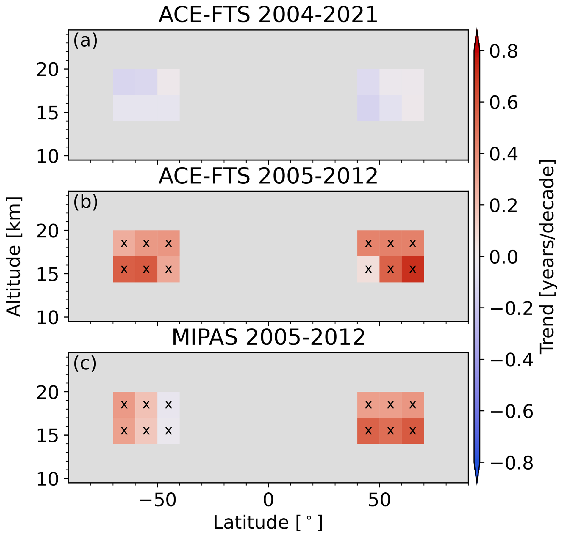
Figure 18 Zonal distribution of the linear trends for (a) age derived from ACE-FTS over the 2004-2021 period, (b) age derived from ACE-FTS over the 2005–2012 period, and (c) age derived from MIPAS over the 2005–2012 period. The crosses indicate where the ACE-FTS 2005–2012 and MIPAS 2005–2012 trends are within 2 standard deviations of each other.

While rigorous trend estimation remains challenging, valuable conclusions can be drawn from the analysis presented in this section. The comparison between the 2005–2012 and the 2004–2021 ACE-FTS trends shows that the linear term is sensitive to the length of the time series. This is expected due to the high variance in the age-of-air datasets; it is difficult to separate natural variability from a long-term trend, especially a small one, with a short time series. The 2004–2021 time series revealed a decadal variation signal in the time series, which appeared as a positive trend for the MIPAS mission period in both the ACE-FTS and MIPAS datasets. This is an example of how natural variability can explain short-term trends, and these trends therefore should not be extrapolated beyond the time period covered by the dataset from which they were inferred. This further demonstrates the importance of a long age-of-air time series. A similar phenomenon was observed by Strahan et al. (2020) in the MIPAS age-of-air data, who showed that the MIPAS time series happens to have been taken during one of the largest oscillations in age of air on record and thus must not be over-interpreted as representative of longer timescales. There are signs of an asymmetric acceleration of the shallow branch of the BDC within both hemispheres if there is no change in tropical age. This is consistent with the decrease in the shallow branch transit time found by Bönisch et al. (2011) over the 1979–2009 period. The decrease in age of air in the 60–70° S bin at 17–20 km would imply that the deep branch is also accelerating in the Southern Hemisphere if tropical ages are constant. A denser age-of-air time series at even higher latitudes would be useful for corroborating whether ages there are decreasing.

6 Summary

An age-of-air dataset was derived from the 17-year ACE-FTS v3.5/3.6 SF₆ time series. The dataset exhibited the expected qualitative pattern based on air motion due to the BDC: air was shown to be older at higher latitudes and altitudes. A correction was applied to account for the influence of the mesospheric SF₆ sink on the calculated age of air; this was found to reduce the derived age and was strongest in polar regions where mesospheric air enters the stratosphere. The ACE-FTS ages displayed the same behaviour as the ages derived from MIPAS, but MIPAS showed significantly older air at higher latitudes and altitudes. The differences were reduced with the sink correction applied to both datasets, but the ages still differed by up to roughly 3 years. However, ACE-FTS age was mostly consistent with ages derived from in situ aircraft measurements, with a few exceptions that could be explained by location sampling differences between the two instruments or by proximity to the tropopause or the polar vortex edge. Comparisons with age of air derived from balloon measurements of SF₆ and CO₂ from before the ACE-FTS mission are consistent with an acceleration of the shallow branch of the BDC and possibly a slowing of the deep branch between 1995 and the mid-2000s, though this was based on comparisons with single balloon flights. Both of these indications would be consistent with previously determined trends in age of air derived from observations or from reanalysis data.

Two applications of the ACE-FTS age-of-air dataset were demonstrated. First, the sink-corrected ages were compared with the age product from CMAM39. It was found that the modelled age was too young compared with the ACE-FTS age, except near the tropical tropopause, which is consistent with previous studies suggesting that the BDC is too fast in the model. The ACE-FTS age-of-air time series was also used for more detailed examination of the trend through regression analysis. While there remain several limitations to this analysis, the results corroborate what has been found in several other studies. Since ACE-FTS uses solar occultation, it has a high signal-to-noise ratio compared to other remote sensing instruments, but the measurements are spatially sparse. This means that there are significantly fewer measurements in each bin in the age dataset and not every month has a corresponding age in a given latitude bin. While the time series are longer than what has been available for age of air until now on a global scale, these attributes make it nevertheless difficult to account for natural variability. In this study it was determined that despite this, including oscillations such as the QBO, ENSO, and a decadal variation approximated by the solar cycle, using respective proxy data, improved the regression analysis. The linear trend was calculated for bins in the middle to high latitudes (40–70°) in the lower stratosphere (14–20 km) because these bins have the most data points and are a meaningful location for examining the BDC. A negative linear trend significant to 2 standard deviations was found in 4 of the 12 bins that were considered – 2 bins in each hemisphere. These results are consistent with an acceleration of the shallow branch of the BDC. Such an acceleration was previously seen by Bönisch et al. (2011) for the 1979–2009 period and Haenel et al. (2015) for the 2002–2012 period in parts of the Southern Hemisphere but without statistical significance. It was also seen by Ray et al. (2014) in the northern midlatitudes. The negative trend found at 60–70° S may also indicate an acceleration of the deep branch of the BDC, which has not previously been seen with observational data. These results agree, at least qualitatively, with climate model predictions of changes in atmospheric circulation. However, they are prone to uncertainty from natural variability, and longer data records are required for increasing reliability of trend estimates.