Invisible aerosol layers: improved lidar detection capabilities by means of laser-induced aerosol fluorescence

One of the most powerful instruments for studying aerosol particles and their interactions with the environment is atmospheric lidar. In recent years, fluorescence lidar has emerged as a useful tool for identifying aerosol particles due to its link with biological content. Since 2022, this technique has been implemented in Leipzig, Germany. This paper describes the experimental setup and data analysis, with a special emphasis on the characterization of the new fluorescence channel centered at 466 nm. The new capabilities of the fluorescence lidar are examined and corroborated through several case studies. Most of the measurement cases considered are from the spring and summer of 2023, when large amounts of biomass-burning aerosol from huge forest fires in Canada were transported to Europe. The fluorescence of the observed aerosol layers is characterized. For wildfire smoke, the fluorescence capacity was typically in the range of $\mathrm{2}\times {\mathrm{10}}^{-\mathrm{4}}$–7 × 10⁻⁴, which aligns well with the values reported in the literature. The key aspects of this study are the capabilities of the fluorescence lidar technique, which can potentially improve not only the typing but even the detection of aerosol particles. In several measurement cases with an apparently low aerosol load, the fluorescence channel clearly revealed the presence of aerosol layers that were not detectable with the traditional elastic-backscatter channels. This capability is discussed in detail and linked to the fact that fluorescence backscattering is related to aerosol particles only. A second area of potential of the fluorescence technique is the distinction between non-activated aerosol particles and hydrometeors, given water's inability to exhibit fluorescence. A smoke–cirrus case study suggests an influence of the aerosol layer on cloud formation, as it seems to affect the elastic-backscatter coefficient within the cloud passing time. These aforementioned applications promise huge advancements towards a more detailed view of the aerosol–cloud interaction problem.

1 Introduction

A crucial player in the atmospheric system comprises aerosol particles, given their role in various processes that ultimately shape the Earth's energy and hydrological budgets. Firstly, aerosol particles scatter and absorb radiation, affecting energy balance on a global scale. By serving as cloud condensation nuclei (CCN) or ice-nucleating particles (INPs), these particles can impact the microphysical properties of clouds (Liu et al., 2014), making them more or less reflective depending on the aerosol situation. In the case of liquid-water clouds, this effect has been largely studied (Twomey, 1974, 1977; Twomey et al., 1984; Quaas et al., 2020), whereas for ice clouds it is a rather new topic (Patnaude and Diao, 2020; Maciel et al., 2023). Because the microphysical properties of a cloud play a major role in its development and the formation of precipitation, aerosol conditions can further affect the extension and lifetime of cloud events and therefore global albedo (Albrecht, 1989; Stevens and Feingold, 2009). Highly absorbing aerosol particles might even affect clouds via the so-called semi-direct effect, which can manifest, for example, in the evaporation of cloud droplets due to an aerosol-heated environment (Hansen et al., 1997). Aerosol effects on the ice phase of cloud formation only complicate the picture. Multiple efforts have been made to analyze the role of aerosol particles as INPs in mixed-phase clouds via heterogeneous freezing and the global effect (Lohmann, 2017). As for cirrus clouds, recent studies suggest that heterogeneous freezing in cirrus clouds, particularly via smoke particles, needs to be explored in more detail (Ansmann et al., 2021; Veselovskii et al., 2022a; Mamouri et al., 2023; Ansmann et al., 2024a, b). To improve our understanding of these complex aerosol–cloud interaction processes, reliable detection and characterization of atmospheric aerosol particles are essential.

Multi-wavelength polarization lidars are powerful tools to detect and characterize aerosol particles. After decades of study, several classification schemes are available in the literature (Floutsi et al., 2023; Groß et al., 2013; Burton et al., 2012), mostly relying on intensive (i.e., concentration-independent) optical properties such as the lidar ratio, particle depolarization ratio and Ångström exponent. However, although clear signatures can be expected for some particle types (e.g., low particle depolarization and low lidar ratios for marine aerosol particles), some limitations remain. Distinguishing between stratospheric smoke and volcanic sulfates and separating between tropospheric smoke and urban pollution remain difficult tasks, as their typical ranges of values for particle depolarization and lidar ratios partially overlap. Additional information, such as the fluorescence of atmospheric aerosol particles, may be required to address these typing difficulties (Veselovskii et al., 2022b).

Laser-induced fluorescence is a well-established technique, serving as the basis of several remote-sensing applications. Fluorescence lidars have been around for a while, but their application has mostly focused on water composition (Palmer et al., 2013; Cadondon et al., 2020) and vegetation (Edner et al., 1994). In the domain of atmospheric research, efforts have mostly been directed towards the detection of single molecules (Mcllrath, 1980; Wang et al., 2021). To investigate the fluorescence of atmospheric aerosol particles, the experiments have been mostly performed through in situ probing (Pinnick et al., 2004; Pan, 2015; Zhang et al., 2019; Kawana et al., 2021). As an example, Pan (2015) analyzed the fluorescence of aerosol particles by measurements with an ultraviolet aerodynamic particle sizer (UV-APS) and reported a spectral range for atmospheric fluorescence of 400 to 650 nm, when excited at 355 nm. A first indication of the observation of atmospheric aerosol fluorescence with lidar came in 2005, when Immler et al. (2005) observed an inelastic-backscatter signal in the water vapor Raman channel (i.e., at 407 nm) that was not produced by Raman scattering. They attributed it to the laser-induced fluorescence emission from biomass-burning (BB) aerosol particles and already linked the aerosol fluorescence to organic compounds. Following this, the first atmospheric fluorescence lidars were set up. Sugimoto et al. (2012) constructed a lidar spectrometer and studied the fluorescence of Asian dust and pollution aerosols in the lower troposphere. The first advanced multi-channel atmospheric lidar system with fluorescence technology was implemented at the Lindenberg observatory of the German Meteorological Service (DWD). Initially, Reichardt (2014) observed atmospheric aerosol fluorescence with a lidar spectrometer that was dedicated to measurements of atmospheric water content. He established the fluorescence capacity as a new intensive aerosol property, which is defined as the ratio of the fluorescence backscatter coefficient to an elastic particle backscatter coefficient. Later, Reichardt et al. (2018) implemented a second spectrometer to measure the laser-induced fluorescence of aerosol particles in the middle and upper troposphere. They characterized the fluorescence of mineral dust and BB aerosol and underlined the capabilities of fluorescence measurements to study aerosol–cloud coexistence by enabling the observation of aerosol particles even inside clouds. Saito et al. (2018) studied the spectral fluorescence of atmospheric pollen with lidar and reported a spectral range of 400 to 600 nm for the fluorescence emission, when excited at 355 nm.

Parallel to the developments in spectrometric fluorescence measurements, a further more easily accessible approach to measuring aerosol fluorescence with a single broadband/discrete lidar channel was pursued. Rao et al. (2018) and Li et al. (2019) used Nd:YAG lasers at 266 nm and 355 nm, respectively, and studied the backscattered light in one elastic-backscatter (at the excitation wavelength) and one fluorescence channel. Both instruments were dedicated to aerosol fluorescence measurements and looked only at the boundary layer. Veselovskii et al. (2020, 2021) extended the concept by adding a single broadband fluorescence channel to an existing multi-wavelength lidar system at Lille, France. They also described a retrieval scheme for the computation of the fluorescence backscatter coefficient out of the signal ratio between the fluorescence and the nitrogen channels. Their observations also confirmed the potential of the fluorescence lidar technique to study aerosol particles inside clouds (Veselovskii et al., 2022a). Veselovskii et al. (2022b) showed that fluorescence measurements can improve the aerosol classification with lidar. They proposed, for the first time, a simple classification scheme that combined the linear depolarization ratio with the fluorescence capacity. With this approach, they were able to discriminate between smoke, mineral dust, pollen and urban aerosol, as pollen and smoke showed significantly higher values of fluorescence capacity than urban aerosol and mineral dust. Reichardt et al. (2023) described a procedure for the absolute calibration of spectrometric fluorescence measurements and proposed a method to correct for the systematic fluorescence error in water vapor measurements with Raman lidar, which is significant for dry and strongly fluorescent aerosol layers. They also emphasized that the spectrum's shape is closely related to the aerosol type. Veselovskii et al. (2023) presented an approach to measure rough fluorescence spectra with a lidar with five discrete broadband fluorescence channels at Moscow, Russia. They reported advancements in aerosol typing with this approach compared to a single fluorescence channel. Smoke and urban aerosol particles could be discriminated even at high relative humidity and in the presence of hygroscopic growth.

In this work, we explore the observational capabilities of an atmospheric fluorescence lidar utilizing measurements performed in Leipzig, Germany, with an upgraded system since 2022. A detailed description of the new experimental setup is provided in Sect. 2. The analysis of several measurement cases is presented in Sect. 3. Our findings corroborate the results obtained by previous studies on the capabilities of fluorescence lidars and deepen the discussion in the field of aerosol studies utilizing fluorescence lidar observations. We discuss a unique new capability that is particular to this measurement approach. Because it is sensitive to particles only, a fluorescence channel can potentially improve not only the typing but even the detection of aerosol particles. Section 3.2.3 provides an in-depth analysis of the reasons for this increased sensitivity of the fluorescence channel to aerosol particles. An exceptional smoke–cirrus interaction case presented in Sect. 3.3 highlights the importance of the ability to detect thin aerosol layers in the upper troposphere and lower stratosphere (UTLS) region for the investigation of cirrus cloud formation. Furthermore, it corroborates and expands the initial work on the detection of fluorescence signals inside ice clouds. The paper concludes in Sect. 4.

2 Experimental setup

2.1 Implementation of a fluorescence channel in the MARTHA lidar system

The Multiwavelength Atmospheric Raman Lidar for Temperature, Humidity, and Aerosol profiling (MARTHA) system is a lab-based lidar system at the Leibniz Institute for Tropospheric Research (TROPOS) in Leipzig. It emits electromagnetic radiation at three wavelengths (355, 532 and 1064 nm) with an overall pulse energy of about 1.2 J at a repetition rate of 30 Hz and collects the backscattered radiation with a large main mirror, which measures 80 cm in diameter. A detailed description of the MARTHA system is given in Mattis et al. (2002), Schmidt et al. (2013) and Jimenez et al. (2019).

To measure the laser-induced fluorescence of atmospheric aerosol, the MARTHA lidar system was upgraded by adding a discrete fluorescence channel to the receiving unit in 2022. To facilitate comparability, the spectral range of the channel was set in the same wavelength range as in Veselovskii et al. (2020). A 44 nm wide interference filter from Alluxa centered at 466 nm is used to select a part of the fluorescence spectrum of fluorescing aerosol particles. Because of their similar features, a first comparison of the results obtained in Lille, France, and Leipzig, Germany, is possible.

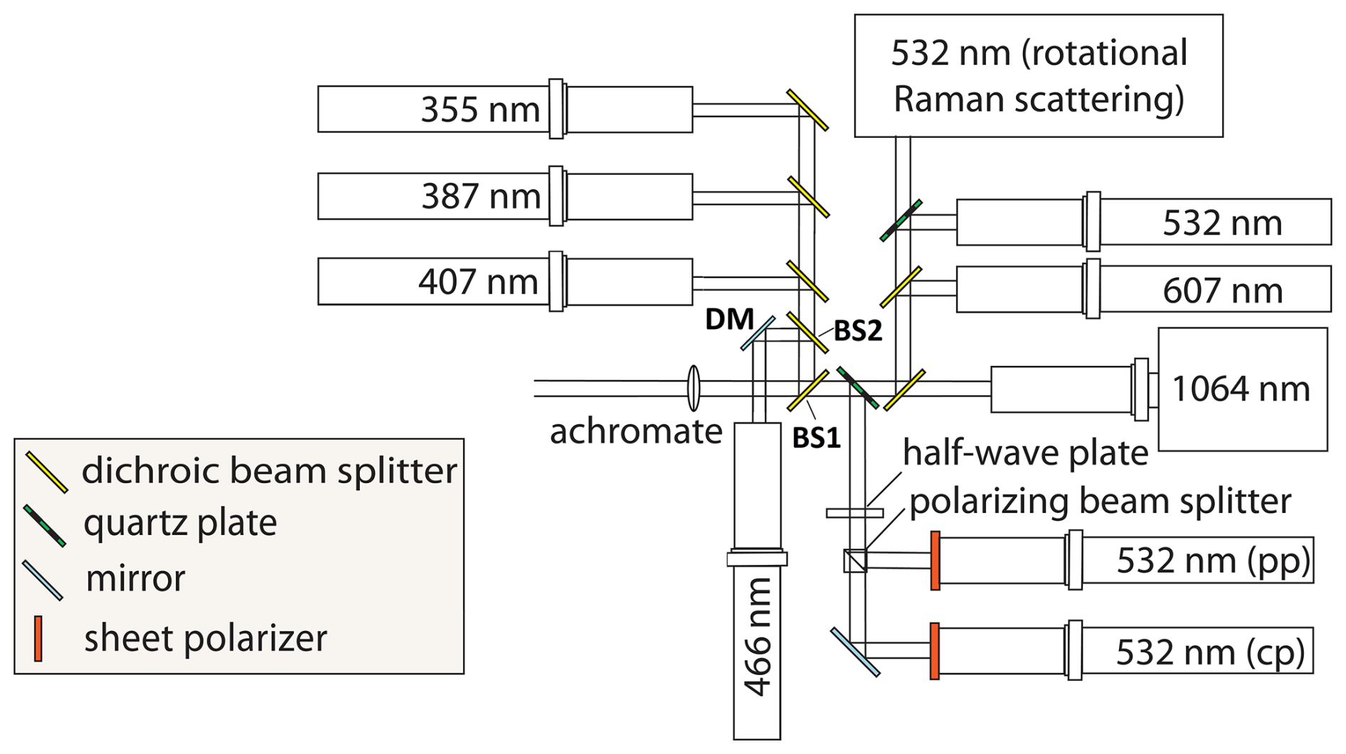
Figure 1 Setup of the far-range receiving unit of the MARTHA system after implementing the fluorescence channel (graphic adapted from Schmidt, 2014). DM: dielectric mirror; BS: beam splitter. pp and cp indicate the channels detecting the parallel-polarized (pp) and cross-polarized (cp) 532 nm signal components with respect to the polarization plane of the transmitted linearly polarized 532 nm laser pulses.

The backscattered fluorescence intensity depends on the aerosol situation, but in general, it is much weaker than elastic-backscatter signals. Therefore, the signal-to-noise ratio in the new channel must be as high as possible. The features that made the MARTHA system suitable to detecting fluorescence are its large telescope area and high-power laser. The second-harmonic-generation and third-harmonic-generation setups allowed an increase in the laser energy at 355 nm, sending 6 ns pulses with an energy of about 350 mJ. The new setup of the MARTHA far-range (FR) receiver, including the fluorescence channel, is displayed in Fig. 1. The new detection channel was placed in the branch with the lower wavelengths. Therefore, the first long-pass beam splitter (BS1) was replaced to ensure the complete reflection of the intended fluorescence spectral band. A second beam splitter (BS2) was added. It transmits the shorter wavelengths to the elastic-backscatter and Raman channels related to the UV laser emission at 355 nm and reflects the longer wavelengths towards the fluorescence channel. As the fluorescence signal can be 4–5 orders of magnitude weaker than elastic backscattering (Veselovskii et al., 2020), sufficient suppression of the elastic returns in the new channel was essential to measure fluorescence. The two new beam splitters received customized coatings from Laseroptik GmbH to guarantee high suppression of the elastic-backscatter (and Raman) lines with minimal loss of fluorescence return. Two interference filters were placed in tandem to suppress the elastic components further.

2.2 Analytical scheme of the fluorescence backscatter coefficient

The lidar system was operated manually and only when no rain was expected. Complete night measurements have been collected since 2022 and were analyzed with a focus on the fluorescing properties of the observed aerosol layers. A second important step is the derivation of new products. The procedure is described as follows: the aerosol fluorescence backscatter coefficient was obtained by forming the ratio of the fluorescence (P_F) to the nitrogen Raman (P_R) signal, similarly to the study of Veselovskii et al. (2020). Both signals can be described in terms of the lidar equations:

$$\begin{array}{}\text{(1)}& {\displaystyle }{P}_{\mathrm{F}}={\mathit{\beta }}_{\mathrm{F}}{T}_{\mathrm{L}}{T}_{\mathrm{F}}{C}_{\mathrm{F}},\text{(2)}& {\displaystyle }{P}_{\mathrm{R}}={\mathit{\beta }}_{\mathrm{R}}{T}_{\mathrm{L}}{T}_{\mathrm{R}}{C}_{\mathrm{R}}.\end{array}$$

T_L is the atmospheric transmission at the emitted laser wavelength. T_R and T_F denote the atmospheric transmission at the Raman and fluorescence wavelength ranges, respectively, and C_R and C_F represent the corresponding lidar calibration constants. By dividing Eq. (1) by Eq. (2), the following expression for the aerosol fluorescence backscatter coefficient β_F can be derived:

$$\begin{array}{}\text{(3)}& {\mathit{\beta }}_{\mathrm{F}}={\displaystyle \frac{P_{\mathrm{F}}}{P_{\mathrm{R}}}}{\displaystyle \frac{T_{\mathrm{R}}}{T_{\mathrm{F}}}}{\displaystyle \frac{C_{\mathrm{R}}}{C_{\mathrm{F}}}}{\mathit{\beta }}_{\mathrm{R}}.\end{array}$$

The Raman backscattering β_R is computed using the following expression in terms of the Rayleigh molecular backscatter coefficient (β_mol):

$$\begin{array}{}\text{(4)}& {\mathit{\beta }}_{\mathrm{R}}=D_{\mathrm{R}}{N}_{{\mathrm{N}}_{\mathrm{2}}}=\mathrm{0.78}{D}_{\mathrm{R}}{N}_{\text{mol}}=\mathrm{0.78}{\displaystyle \frac{D_{\mathrm{R}}}{D_{\text{mol}}}}{\mathit{\beta }}_{\text{mol}},\end{array}$$

with $N_{{\mathrm{N}}_{\mathrm{2}}}$ and N_mol being the number density of nitrogen and air molecules, respectively. $D_{\mathrm{R}}/D_{\text{mol}}$ accounts for the ratio of the Raman to Rayleigh backscatter differential cross section. These cross sections were determined theoretically using Eqs. (20) and (14) in Adam (2009), resulting in theoretical values of D_R = 2.7344 × 10⁻³⁴ and D_mol = 3.10875 × 10⁻³¹ m² sr⁻¹.

2.3 Technical considerations for the calibration of the fluorescence channel

To derive the particle fluorescence backscatter coefficient from Eq. (3), the traditional method, using a particle-free reference height, cannot be applied, due to the unknown fluorescence response of the background aerosol. Instead, a characterization of the channel's system efficiencies is needed. The contribution of each component in the respective detection path was carefully determined to infer the overall efficiencies and build the lidar-constant ratio $C_{\mathrm{R}}/C_{\mathrm{F}}$.

Table 1 Transmittances 𝒯 or reflectances ℛ of all optical elements in the 387 and 466 nm FR channels. The photomultiplier tube (PMT) quantum efficiencies, PMT gain ratio and overall ratio of the lidar calibration constants in both channels are given.

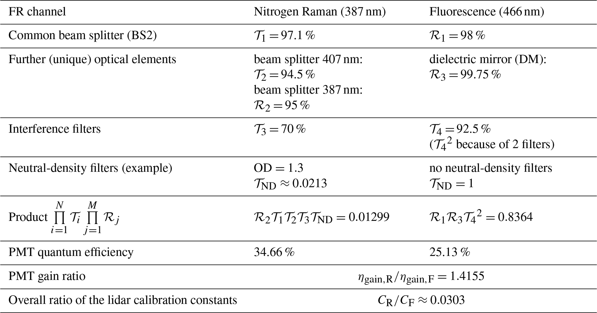
The first point to consider is the bandwidth of the interference filters. For the 387 nm nitrogen Raman channel, with a bandwidth of 2.7 nm, only 95 % of the theoretical Raman cross section can reach the detector, reducing the actual cross section at the detector to $D_R=\mathrm{0.95}\times \mathrm{2.7344}\times {\mathrm{10}}^{-\mathrm{34}}$ m² sr${}^{-\mathrm{1}}=\mathrm{2.59768}\times {\mathrm{10}}^{-\mathrm{34}}$ m² sr⁻¹. This value is then used in Eq. (4) together with the molecular backscatter computed based on the temperature and pressure profiles provided by the Global Data Assimilation System (GDAS) (Rodell et al., 2004) to derive the Raman backscatter coefficient. As the laser power, pulse length and telescope area are the same for both detection channels, the lidar-constant ratio $C_{\mathrm{R}}/C_{\mathrm{F}}$ is simplified to the ratio of the channel efficiencies. This ratio comprises the transmittances or reflectances of the optical elements (such as beam splitters, mirrors, interference filters and neutral-density filters) and the detection efficiencies of the detectors. The transmittances and reflectances of the optical components are collected in Table 1. As the neutral-density (ND) filters are eventually changed depending on the atmospheric and system conditions, only the optical depth (OD) of one exemplary set of ND filters, which is representative of most of the cases studied in this paper, was chosen for Table 1. When determining the ND filter transmission, the spectral dependence provided by the manufacturer (Thorlabs) was considered. The detection efficiencies of the photomultiplier tubes (PMTs) are split into electrical gain and detector efficiency. The ratio of the electrical gains was obtained by swapping the detectors in the nitrogen Raman and fluorescence channels and forming the ratio of the mean signals measured by both detectors for each channel. This test yielded a PMT gain ratio (${\mathit{\eta }}_{\text{gain},\mathrm{R}}/{\mathit{\eta }}_{\text{gain},\mathrm{F}}$) of 1.4155, indicating a higher gain of the nitrogen Raman channel's PMT. As for the detector surface, the so-called quantum efficiency accounts for the quantity of photoelectrons generated by the cathode divided by the number of incident photons. This efficiency depends on the photon wavelength (Wright, 2017). The spectrally resolved quantum-efficiency data provided by Hamamatsu were considered to assess the PMT type used in the MARTHA system. The maximum efficiency of the detectors is about 35 %, and the values at the wavelength ranges of the two lidar channels were determined by interpolation from the provided data points and averaging over the filter width of the interference filter in the fluorescence channel. This resulted in values of η_qe,R = 34.66 % and η_qe,F = 25.13 % for the quantum efficiencies of the PMT type used in the nitrogen Raman (386–388 nm) and fluorescence (444–488 nm) channels, respectively, and we finally obtained a ratio of ${\mathit{\eta }}_{\text{qe},\mathrm{R}}/{\mathit{\eta }}_{\text{qe},\mathrm{F}}=\mathrm{1.379}$.

After these considerations, the ratio of the lidar calibration constants can be calculated from the efficiency ratios of the optical elements, detector gain and spectral response as follows:

$$\begin{array}{}\text{(5)}& {\displaystyle \frac{C_{\mathrm{R}}}{C_{\mathrm{F}}}}={\displaystyle \frac{{\mathcal{R}}_{\mathrm{2}}{\mathcal{T}}_{\mathrm{1}}{\mathcal{T}}_{\mathrm{2}}{\mathcal{T}}_{\mathrm{3}}{\mathcal{T}}_{\text{ND}}}{{\mathcal{R}}_{\mathrm{1}}{\mathcal{R}}_{\mathrm{3}}{{\mathcal{T}}_{\mathrm{4}}}^{\mathrm{2}}}}{\displaystyle \frac{{\mathit{\eta }}_{\text{gain},\mathrm{R}}}{{\mathit{\eta }}_{\text{gain},\mathrm{F}}}}{\displaystyle \frac{{\mathit{\eta }}_{\text{qe},\mathrm{R}}}{{\mathit{\eta }}_{\text{qe},\mathrm{F}}}}.\end{array}$$

For the set of ND filters considered in Table 1 (OD of 1.3 in the nitrogen Raman and no ND filters in the fluorescence channel), it results in a value of $C_{\mathrm{R}}/C_{\mathrm{F}}\approx \mathrm{0.0303}$.

The remaining unknown in Eq. (3) is the ratio $T_{\mathrm{R}}/T_{\mathrm{F}}$ of the atmospheric transmissions (ground to target) at the Raman and fluorescence wavelengths, respectively. The molecular part ($T_{\mathrm{R}}/T_{\mathrm{F}}{\mathrm{|}}_{\text{mol}}$) is calculated straightforwardly from the extinction and backscatter coefficients; the aerosol contribution to the transmission ratio ($T_{\mathrm{R}}/T_{\mathrm{F}}{\mathrm{|}}_{\text{par}}$) requires previous knowledge of the aerosol backscatter coefficient. For the profile-based analysis, the aerosol optical properties are determined with the traditional Raman technique (Ansmann et al., 1990, 1992). The particle backscatter coefficient at high temporal resolution was obtained via a constant-based approach, in which a previous profile-based retrieval is needed to calculate the lidar constants, which are then used to compute high-resolution products out of the elastic-backscatter and Raman signals (Baars et al., 2017). In general, the particle atmospheric transmission differs little at the two wavelengths, making the effect on the fluorescence backscatter coefficient small, partially because only about 80 nm separates the central wavelengths of the Raman and fluorescence channels. For the cases with low and medium aerosol loads (see Sect. 3.2), the error in the case of non-consideration of the differential transmission was in the range of 2 %–6 %. In the case of an unusually high aerosol optical depth, like on 4 July 2023 (see Sect. 3.1), the error was on the order of 10 %. Thus, the differential particle transmission at the two wavelengths was considered to guarantee the quality of the fluorescence backscatter coefficient, even above strongly backscattering aerosol layers. But still, the assumption of an appropriate Ångström exponent is necessary, which imposes an uncertainty of ± 1 %–7 % on the determined $T_{\mathrm{R}}/T_{\mathrm{F}}{\mathrm{|}}_{\text{par}}$, depending on the optical thickness of the present aerosol layers.

The data set acquired in Leipzig was then analyzed in a semi-automatic manner, setting the calibration constants and the reference height (particle-free) manually for each case. The fluorescence capacity G_F,

$$\begin{array}{}\text{(6)}& G_{\mathrm{F}}={\displaystyle \frac{{\mathit{\beta }}_{\mathrm{F}}}{{\mathit{\beta }}_{\mathrm{532}}}},\end{array}$$

was calculated as the ratio of the fluorescence backscatter coefficient (β_F) to the elastic particle backscatter coefficient at 532 nm (β₅₃₂). To improve comparability with different setups (fluorescence lidars which do not deploy the second-harmonic-generation wavelength and/or use a spectrometric approach or broadband fluorescence channels with different interference filter bandwidths), the general and season-mean values are also provided as spectral fluorescence capacity with respect to the third-harmonic-generation wavelength 355 nm ($G_{\mathrm{F}}^{\mathrm{355}}$),

$$\begin{array}{}\text{(7)}& G_{\mathrm{F}}^{\mathrm{355}}={\displaystyle \frac{{\mathit{\beta }}_{\mathrm{F}}}{{\mathit{\beta }}_{\mathrm{355}}{d}_{\text{IF}}}},\end{array}$$

where d_IF = 44 nm is the bandwidth of the interference filter in the fluorescence channel. Furthermore, data from the collocated portable Raman lidar Polly^XT (Engelmann et al., 2016) at TROPOS were used to provide quality-assured depolarization profiles.

3 Observational results

Due to the broad bandwidth of the fluorescence channel and the low intensity of the fluorescence signal, measurements were only possible during the night. In the daytime, scattered solar radiation would cause too much noise in the fluorescence channel. As the MARTHA system is operated manually, the number of measurements remains limited. Since August 2022, about 50 measurements have been performed, providing more than 250 h of atmospheric fluorescence observations. Typical atmospheric values of the fluorescence backscatter coefficient and fluorescence capacity, which were obtained at Leipzig during the time period from August 2022 to October 2023, are presented in the next paragraph.

In general, β_F ranged between 1 × 10⁻⁵ ${\mathrm{Mm}}^{-\mathrm{1}}{\mathrm{sr}}^{-\mathrm{1}}$ for background aerosol and more than 1 × 10⁻³ ${\mathrm{Mm}}^{-\mathrm{1}}{\mathrm{sr}}^{-\mathrm{1}}$ for optically extraordinarily thick wildfire smoke layers. Correspondingly, G_F ($G_{\mathrm{F}}^{\mathrm{355}}$) varied from ∼ 10⁻⁶ (∼ 10⁻⁸ nm⁻¹) for clouds and 1 × 10⁻⁵ (1 × 10⁻⁷ nm⁻¹) for background aerosol to 1.3 × 10⁻³ (1.3 × 10⁻⁵ nm⁻¹), whereas most of the measurement points were in the range of 5 × 10⁻⁵ to 7 × 10⁻⁴ (6 × 10⁻⁷ to 9 × 10⁻⁶ nm⁻¹). That is, the fluorescence backscatter coefficient was about 4 orders of magnitude lower than the elastic ones, which agrees with the findings by Veselovskii et al. (2020).

In the following, four interesting case studies are presented in several subsections. In Sect. 3.1, the fluorescence properties of wildfire smoke are discussed by analyzing an optically and geometrically thick smoke layer on 4 July 2023. In Sect. 3.2, we first demonstrate the ability of the fluorescence lidar technique to detect optically thin aerosol layers by presenting two case studies (Sect. 3.2.1 and 3.2.2). Subsequently, we discuss the reasons for the increased sensitivity of the fluorescence channel to aerosol particles in Sect. 3.2.3. Finally, we underline the importance of this new capability by presenting a striking smoke–cirrus interaction case study in Sect. 3.3.

3.1 Fluorescence of wildfire smoke – 4 July 2023

In the spring and summer of 2023, huge wildfires raged across Canada, with unusual intensity in the provinces of Alberta and British Columbia. With the prevailing westerly winds, large amounts of biomass-burning aerosol were transported towards Europe. As a result, we frequently observed wildfire smoke layers over Leipzig from mid-May to mid-July 2023.

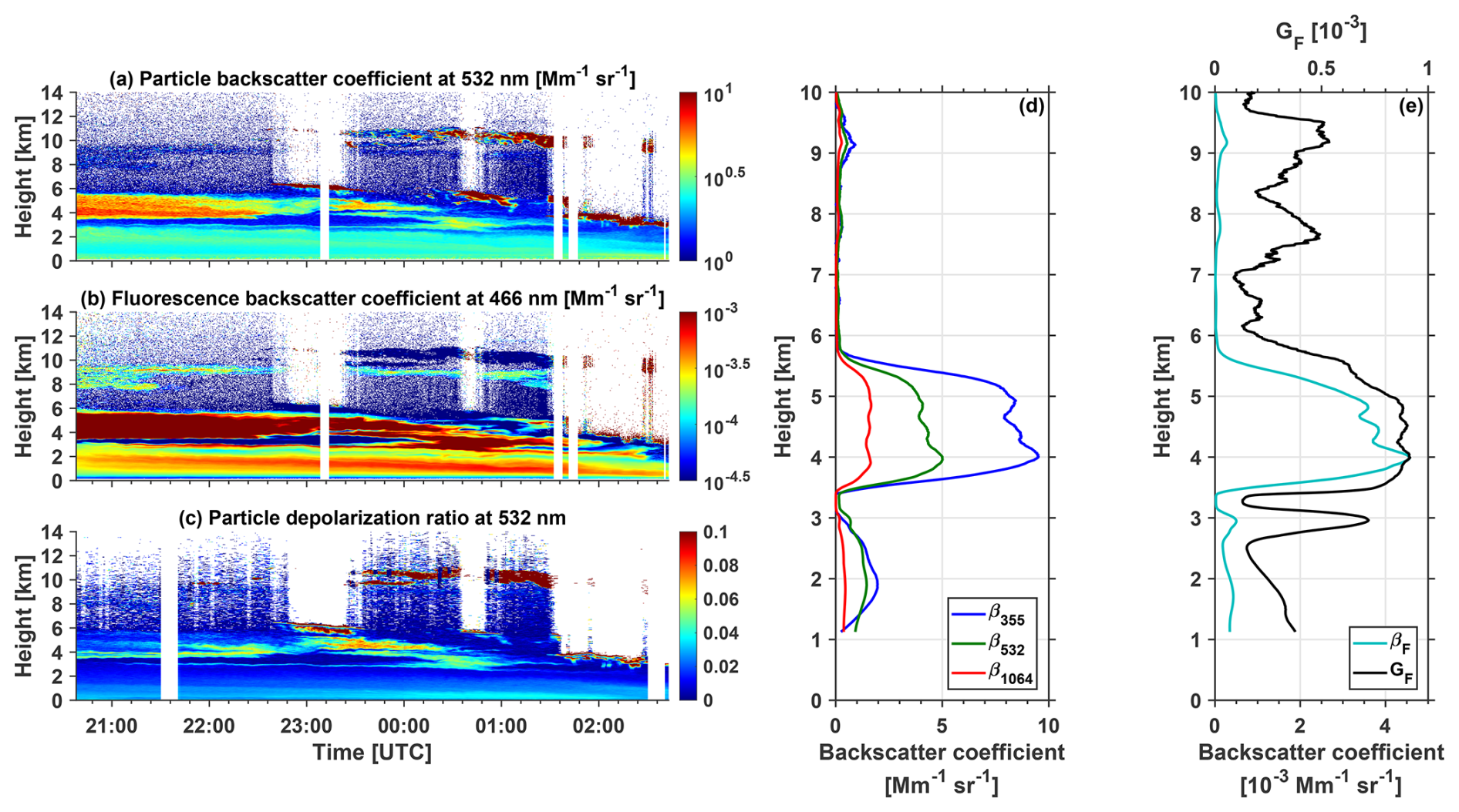
Figure 2 Height–time distributions of (a) the particle backscatter coefficient at 532 nm and (b) the fluorescence backscatter coefficient (β_F) measured with the MARTHA system and (c) the particle depolarization ratio at 532 nm from Polly^XT on 4–5 July 2023. Vertical profiles of (d) the elastic-backscatter coefficients and (e) β_F are shown together with the fluorescence capacity (G_F) from 21:00 to 22:00 UTC on 4 July 2023.

As a first example, the fluorescence of an optically thick plume of wildfire smoke on 4–5 July 2023 shall be characterized. Figure 2 displays the height–time distributions of the particle backscatter coefficient at 532 nm, the fluorescence backscatter coefficient and the particle depolarization ratio at 532 nm for this night. Figure 2a shows a highly polluted troposphere, with an overall aerosol optical depth (AOD) of around 0.8 at 532 nm. This agrees well with data from the Aerosol Robotic Network (AERONET, 2024), where AOD values of around 0.75–0.8 were retrieved at 500 nm at 17:00 UTC on 4 July 2023. An optically thick aerosol layer extended from 3.4 to 5.8 km height. To determine its optical properties, a 1 h time period was considered for temporal averaging. Figure 2d and e show the vertical profiles of the fluorescence and elastic-backscatter coefficients, together with the fluorescence capacity averaged over the time period from 21:00 to 22:00 UTC. At the optically thickest part, β₅₃₂ reached values of up to 5 ${\mathrm{Mm}}^{-\mathrm{1}}{\mathrm{sr}}^{-\mathrm{1}}$. The 532 nm AOD of the whole layer amounted to around 0.48.

The optical properties of this aerosol layer, ranging from 3.4 to 5.8 km height, were then used to determine the aerosol type. The lidar ratio at 532 nm (60 sr) was significantly larger than the one at 355 nm (38 sr), and the backscatter-related Ångström exponent was high (1.66). These values are characteristic for aged BB aerosol (Müller et al., 2005; Ansmann et al., 2009; Ohneiser et al., 2021, 2022; Hu et al., 2022; Janicka et al., 2023). Furthermore, these retrieved lidar ratio values are in the same range as reported for aged wildfire smoke in previous studies (e.g., Murayama et al., 2004; Ansmann et al., 2009; Haarig et al., 2018; Hu et al., 2019). The low particle depolarization ratio (δ₅₃₂≤0.07; see Fig. 2c) in the layer from 3.4 to 5.8 km height points to a spherical shape of the particles, which is also typical of aged wildfire smoke in the middle free troposphere (Haarig et al., 2018). Thus, it can be concluded that this tropospheric aerosol layer consisted of aged BB aerosol particles.

Figure 2b and e show a very high layer-mean fluorescence backscatter coefficient (β_F≈ 2.75 × 10⁻³ ${\mathrm{Mm}}^{-\mathrm{1}}{\mathrm{sr}}^{-\mathrm{1}}$) for this smoke layer and a corresponding layer-mean fluorescence capacity of G_F≈ 7.8 × 10⁻⁴. In other words, smoke shows very high values of fluorescence capacity compared to other particle types and can thus be clearly identified through this new quantity. These values witnessed in our observations agree with the findings by Veselovskii et al. (2020).

Considering the entire 2023 wildfire season, the fluorescence capacity G_F (spectral fluorescence capacity $G_{\mathrm{F}}^{\mathrm{355}}$) of smoke varied from 1 × 10⁻⁴ to 13 × 10⁻⁴ (1.5 × 10⁻⁶ to 13 × 10⁻⁶ nm⁻¹). Thereby, values of 2 × 10⁻⁴–7 × 10⁻⁴ (2 × 10⁻⁶–9 × 10⁻⁶ nm⁻¹) were observed most frequently, which agrees with the results of Hu et al. (2022) and Veselovskii et al. (2022a), who reported values of G_F in the range of 1 × 10⁻⁴–4.5 × 10⁻⁴ for their observations at Lille, France. The observed values of $G_{\mathrm{F}}^{\mathrm{355}}$ are also in a range similar to the spectral fluorescence capacities of BB aerosol that were reported by Reichardt et al. (2018), although for a broader wavelength range (455–530 nm). The particle depolarization ratio at 532 nm was low (below 0.07) for most (95 %) of the investigated smoke layers.

3.2 Detection of optically thin aerosol layers with the fluorescence channel

Besides its relevance for aerosol type identification, our results suggest an additional capability of a fluorescence lidar: to detect optically thin aerosol layers. In several measurements with the new fluorescence channel, an enhanced fluorescence signal revealed the presence of aerosol layers that went unnoticed when employing only the elastic-backscatter detection channels. Three exemplary measurement cases are discussed in the following sections.

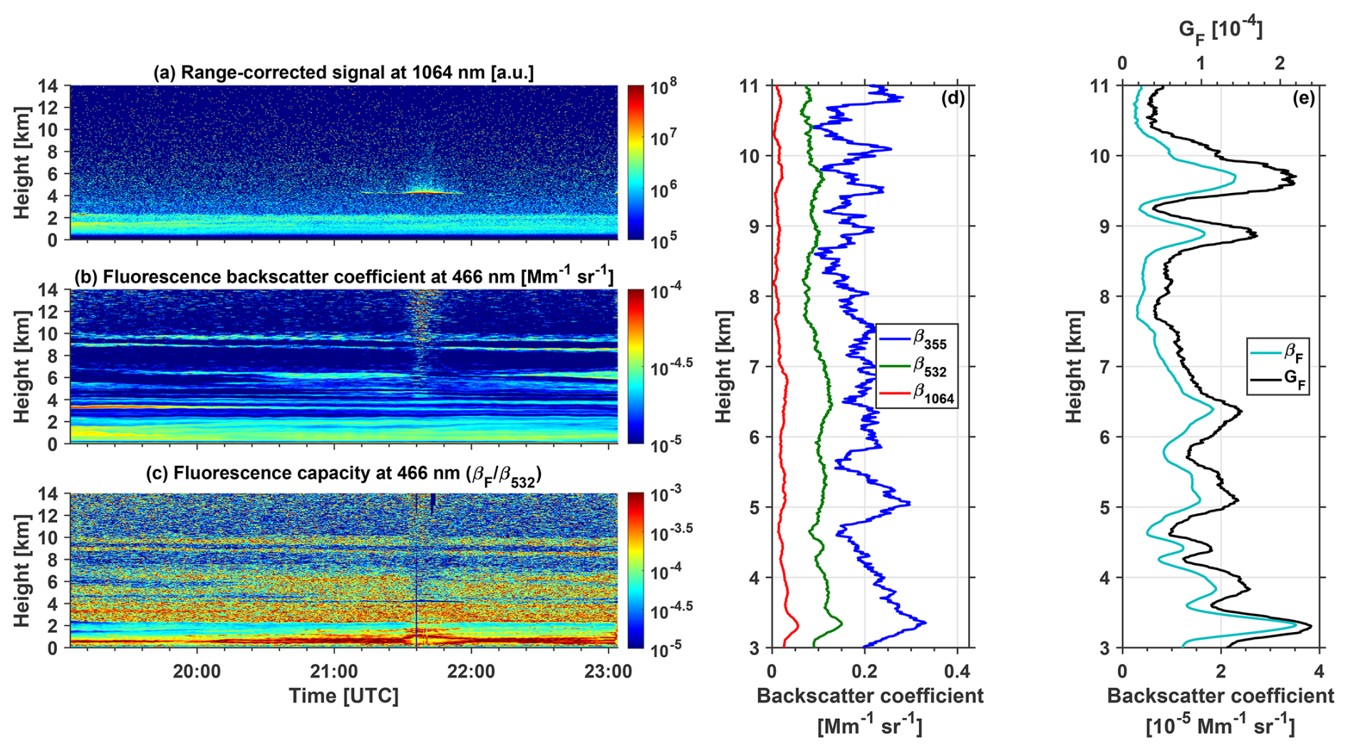
Figure 3 Height–time distributions of (a) the range-corrected lidar signal at 1064 nm, (b) the fluorescence backscatter coefficient (β_F) and (c) fluorescence capacity measured with the MARTHA system on 21 September 2022. Vertical profiles of (d) the elastic-backscatter coefficients and (e) β_F are shown together with the fluorescence capacity (G_F) from 19:04 to 21:04 UTC on 21 September 2022.

3.2.1 Hidden smoke layers – 21 September 2022

Figure 3 shows the height–time distributions of the range-corrected lidar signal at 1064 nm (Fig. 3a), the fluorescence backscatter coefficient (Fig. 3b) and the fluorescence capacity (Fig. 3c). According to the elastic-backscatter signal in Fig. 3a, the upper troposphere appears to be rather aerosol-free. Only the polluted boundary layer and some thin layers up to 4 km height indicated an aerosol presence, and a thin cloud was visible at around 4 km height from 21:00 to 22:00 UTC. However, an enhanced fluorescence backscatter coefficient in Fig. 3b reveals several other fluorescing aerosol structures throughout the middle and upper troposphere (at around 5, 6.5, 9 and 9.75 km height). This already illustrates that with measurements of aerosol fluorescence, thin aerosol layers can be identified more easily from lidar quicklooks and therefore chosen for detailed analysis. Looking at the vertical profiles, this measurement case appears even more impressive. Figure 3d and e display the time-averaged vertical profiles of the fluorescence and elastic-backscatter coefficients together with the fluorescence capacity. The profiles were averaged over the 2 h time period from 19:04 to 21:04 UTC to exclude the cloud, which was present at around 4 km height from that point onwards. The lowest (3.3 km) and most fluorescent (β_F≈ 2.5 × 10⁻⁵ ${\mathrm{Mm}}^{-\mathrm{1}}{\mathrm{sr}}^{-\mathrm{1}}$) layer above the boundary layer still shows clearly enhanced elastic-backscatter coefficients at all three wavelengths. In the mid-level layers at around 5 and 6.5 km height, the 532 nm and 1064 nm backscatter coefficients are only slightly enhanced compared to the background. For the layer at 6.5 km height, their corresponding maxima are at higher altitudes than the distinct maximum in the fluorescence backscatter coefficient. The 355 nm backscatter coefficient even fails to resolve the aerosol layer at 6.5 km. However, all elastic-backscatter detection channels reach their limits with the two high layers at 9 and 9.75 km altitude. While the 355 nm backscatter coefficient is completely noisy in this altitude range, β₅₃₂ and β₁₀₆₄ do show maxima in the altitude range of the increased β_F. But these maxima are difficult to distinguish from the background, which is likewise already quite noisy. Thus, it is unlikely that these two higher layers would have been detected as aerosol layers without the additional fluorescence information, especially because the particle depolarization ratio (not shown) is also quite low, around 2 %.

The overall AOD of this measurement case was around 0.13 at 532 nm, which is consistent with AERONET data (AERONET, 2024) showing 0.1 at 500 nm, whereas the majority of the aerosol was found in the boundary layer (AOD ≈ 0.1). The smoke layers above the boundary layer only added up to an AOD of around 0.03. The two thinnest layers at around 9 and 9.75 km height even had an AOD of only 0.002 each at 532 nm.

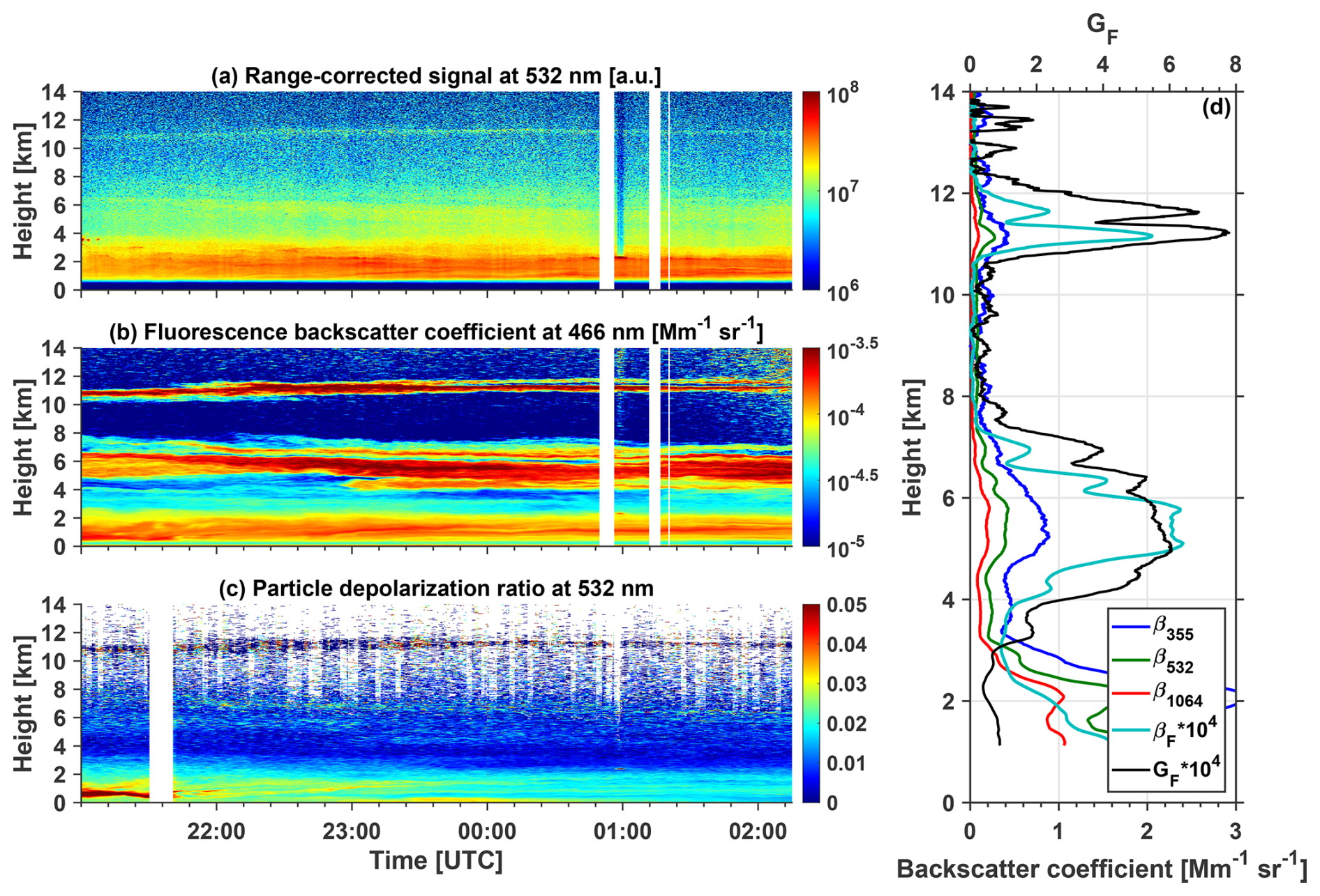
Figure 4 Height–time distributions of (a) the range-corrected lidar signal at 532 nm and (b) the fluorescence backscatter coefficient (β_F) measured with the MARTHA system and (c) the particle depolarization ratio at 532 nm from Polly^XT on 15–16 May 2023. (d) Vertical profiles of β_F and the elastic-backscatter coefficients are shown together with the fluorescence capacity (G_F) from 01:15 to 02:15 UTC on 16 May 2023.

3.2.2 A thin smoke layer in the UTLS – 15 May 2023

Another example of such “unnoticeable” layers is the night of 15–16 May 2023. Figure 4a–c display the height–time distributions of the range-corrected lidar signal at 532 nm, the fluorescence backscatter coefficient and the particle depolarization ratio at 532 nm. The vertical profiles of the backscatter coefficients together with the fluorescence capacity for the period of 01:15–02:15 UTC are shown in Fig. 4d. This measurement case is characterized by pronounced fluorescent aerosol layers (532 nm AOD ≈ 0.05), ranging from 4 to 6.7 km height. The high fluorescence capacity and lidar ratio values allow us to identify the aerosol particles present as wildfire smoke. For further discussion, we consider a height-constant and rather homogeneous layer, ranging from 4.6 to 6.1 km (layer 1). Layer 1 shows a mean fluorescence capacity of around 5.6 × 10⁻⁴ and lidar ratios of around 40 sr at 355 nm and 70 sr at 532 nm. The particle depolarization ratio at 532 nm is low (around 1.7 %), indicating a well-advanced aging process of the smoke particles. At around 11 km height, the range-corrected signal at 532 nm in Fig. 4a shows another highly fluorescent smoke layer (G_F≈ 6.5 × 10⁻⁴), which we will refer to as layer 2 in the following. This higher value of the fluorescence capacity indicates a more efficient fluorescence emission in layer 2 than in layer 1. The reason for this remains unclear. On the one hand, this could be purer smoke, while layer 1 could also contain a small proportion of another less fluorescent aerosol type. On the other hand, the BB aerosol in both layers could differ in chemical composition and optical properties due to different fire sources and transport mechanisms. Backward trajectory analyses point generally to the same source region (the northern part of the North American continent) for both altitudes. However, this does not exclude the possibility of slightly different fire sources. The optical properties of the smoke particles differ slightly between the two layers. The lidar ratios in layer 2 (55 sr at 355 nm and 75 sr at 532 nm) are slightly higher than the lidar ratios in layer 1. Furthermore, in layer 2, the particle depolarization ratio was slightly enhanced (δ₅₃₂≈ 6.5 %) compared to layer 1, indicating a more irregular shape of the smoke particles in layer 2 (although in general terms this is still almost spherical). The particle size seems to play a minor role in depolarization in this case, as the backscatter-related Ångström exponent for the 355 and 532 nm wavelength pair (1.75 for layer 1 and 1.55 for layer 2) indicates only slightly larger particles in layer 2.

All in all, these differences in aerosol optical properties suggest different fire sources and/or transport mechanisms for both smoke layers. The observed difference in fluorescence capacity is therefore expectable, but its cause remains unclear.

Furthermore, Fig. 4b reveals another aerosol layer (layer 3) with enhanced fluorescence at around 11.7 km, directly above layer 2. The complete structure of layer 3 remains unnoticed in the range-corrected signal in Fig. 4a. This impression is confirmed by the vertical profiles in Fig. 4d. Layer 3, being thin, cannot be distinguished from the background noise in β₃₅₅. β₅₃₂ and β₁₀₆₄ exhibit a slight increase, although this increase is only very weakly pronounced at 1064 nm. Therefore, only the 532 nm backscatter coefficient shows a clear peak for layer 3. At a closer look, the time–height distribution of the particle depolarization ratio at 532 nm in Fig. 4c also indicates layer 3 by slightly increased values at this altitude. But again, it would have been hard to recognize this layer from the elastic-backscattering products alone without having a clearer picture of the aerosol situation from the fluorescence channel. This underlines the potential of the fluorescence lidar technique beyond aerosol characterization. Fluorescence backscatter can be used for the detection of aerosol layers in scenarios where concentrations are below the lower detection limit of the elastic-backscatter channels.

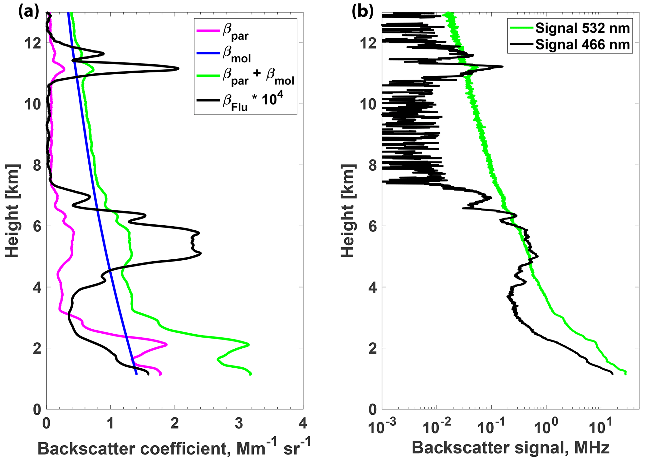
Figure 5 Vertical profiles of (a) particle (magenta), molecular (blue) and total (green) backscatter coefficients at 532 nm and the fluorescence backscatter coefficient (black) and (b) background-corrected signals at 532 nm (green) and 466 nm (black) on 16 May 2023 for the time period from 01:15 to 02:15 UTC.

3.2.3 On the capabilities of a dedicated (aerosol) fluorescence channel

The measurement cases presented demonstrate the advantages of adding fluorescence observations to the analysis. The following paragraph discusses the enhanced capabilities of a fluorescence backscatter channel compared to the classical elastic-backscatter channel.

The three elastic-backscatter channels rely on the principle of elastic backscattering of the emitted laser radiation, which occurs at both air molecules and aerosol particles. Because of the strong decrease in air and aerosol density, the scattering intensity strongly decreases with height. In addition, the backscatter detected by the lidar further decreases with height due to the solid angle of the telescope and atmospheric extinction. As a result, the lidar-signal detection needs to cover a wide dynamic range. Elastic signals are usually attenuated in the detection unit to keep them in a manageable range for a single channel. This maximizes the vertical coverage but at the expense of sensitivity to aerosol particle changes.

A fluorescence channel is dedicated to aerosol particles only. Thus, it can help to increase the sensitivity to aerosol particles by eliminating the molecular component. Furthermore, the fluorescence return scales not only to the number of particles but also to its cross section, which is directly related to the fluorescence capacity of the aerosol particles. That is, a smoke layer will contrast more than a dust layer with the background because of the higher ability of smoke particles to fluoresce. This feature enhances the capabilities of such a channel to detect smoke particles in the atmosphere.

Figure 5a illustrates this context by showing the molecular, particle and total (molecular + particle) backscatter coefficient at 532 nm for a measurement on 16 May 2023. The contrast between the smoke layer (4–7 km) and the background aerosol (8–10 km) in the fluorescence backscatter is significantly more pronounced than in the elastic particle backscatter coefficient. The enhanced detection ability in the case of fluorescing aerosol particles becomes evident when comparing the observed lidar signals (background-corrected), as depicted in Fig. 5b for this measurement case. Especially the aerosol layers at around 11 km stand out much more clearly from the background in the fluorescence signal than in the elastic signal.

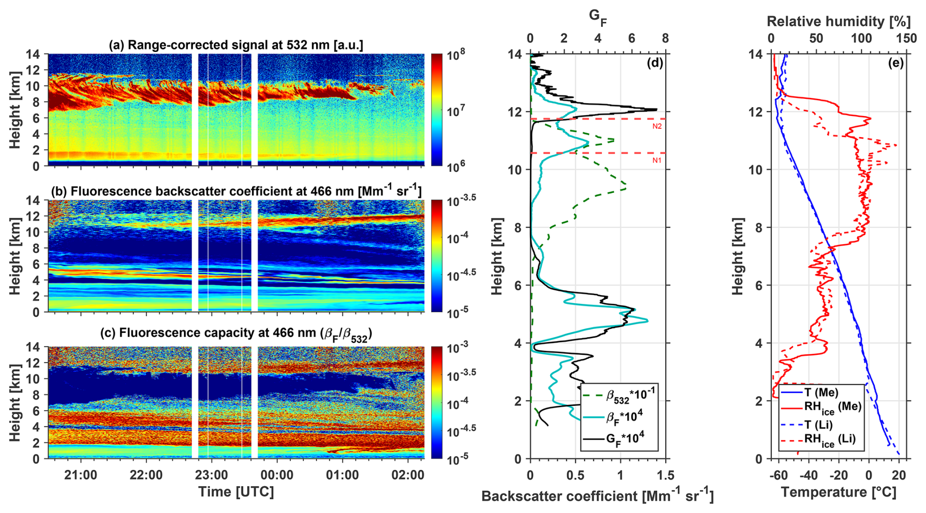
Figure 6 Height–time distributions of (a) the range-corrected lidar signal at 532 nm, (b) the fluorescence backscatter coefficient (β_F) and (c) the fluorescence capacity measured with the MARTHA system on 29–30 May 2023. (d) Vertical profiles of β_F and the elastic-backscatter coefficient at 532 nm together with the fluorescence capacity (G_F) from 21:00 to 22:00 UTC on 29 May 2023. (e) Vertical profiles of temperature (blue curves) and relative humidity over ice (red curves) from radiosoundings launched at Lindenberg at 16:45 UTC on 29 May 2023 (dashed) and Meiningen at 22:45 UTC on 29 May 2023 (solid).

3.3 Atmospheric implication: smoke–cirrus interaction – 29 May 2023

Now, after discussing the possibility of detecting such thin aerosol layers, the question of their relevance in atmospheric research arises. Because of their low optical thicknesses (of typically ≤0.01), such aerosol layers might not have a relevant radiative effect, but the aerosol particles may impact cloud formation, e.g., by serving as INPs. In both cases presented above (Sect. 3.2.1 and 3.2.2), the measurements of the fluorescence backscatter coefficient revealed thin wildfire smoke layers at rather high altitudes around the tropopause. This altitude range, also referred to as the UTLS region, is a common site for the formation of cirrus clouds. However, the ability and relevance of smoke particles to act as INPs comprise an open question in the literature. Although a few available observations showed enhanced immersion-mode INP concentrations inside BB aerosol plumes (Barry et al., 2021; McCluskey et al., 2014), wildfire smoke is considered to be a rather inefficient INP at temperatures above −30 °C compared to other aerosol types such as dust (e.g., Barry et al., 2021; Knopf et al., 2018). Thus, BB aerosol is, in general, not considered a relevant INP source in mixed-phase cloud processes. Likewise, in situ assessments have suggested that BB aerosol particles rarely freeze to form cirrus clouds (Froyd et al., 2009, 2010). However, the authors could not exclude the INP ability of BB particles due to temperature limitations in their experimental setup. Recent lidar-based studies have discussed the potential of smoke particles to promote freezing via deposition and have provided evidence of BB aerosol acting as the main INP source in cirrus clouds observed at Limassol, Cyprus (Mamouri et al., 2023), and in the Arctic (Ansmann et al., 2024a, b). Simulations considering gravity waves further explain how heterogeneous freezing overtakes the main role, quickly consuming the water vapor and reducing supersaturation and hampering in this way homogeneous freezing (Ansmann et al., 2024a). Thus, investigations of possible smoke–cirrus interactions in the UTLS region are an important topic for future studies. Several of our measurement cases during the 2023 wildfire season showed cirrus clouds directly below thin smoke layers. One example (29–30 May 2023) is displayed in Fig. 6 and will be discussed in the following.

The range-corrected lidar signal at 532 nm in Fig. 6a shows cirrus clouds that extended from 7 to 11.5 km at the beginning of the measurement. Above, enhanced values of the fluorescence backscatter coefficient (see Fig. 6b) reveal the presence of a smoke layer at 10.5 to 12 km height that was not visible in the elastic-backscatter lidar signal over large parts of the observation period. Only at the end of this measurement (around 02:00 UTC), when the clouds became thinner and more scattered, could the aerosol layer be anticipated vaguely from weak signatures in the range-corrected signal (see Fig. 6a).

The time–height plot of the fluorescence capacity in Fig. 6c reveals another feature of fluorescence backscattering that is exclusive to aerosol particles. Pure water does not fluoresce, and, as our measurements from 2022–2023 showed, hydrometeors such as cloud droplets and ice crystals exhibit the lowest values of fluorescence capacity. In combination, elastic-backscatter and fluorescence channels can unambiguously differentiate aerosol particles and hydrometeors that coexist within the same air volume. This feature has also been pointed out in previous studies (Reichardt et al., 2018; Veselovskii et al., 2022a) and opens a new door to aerosol and cloud detection.

Due to this characteristic, the fluorescence capacity clearly shows the positions of the aerosol and cloud layers relative to each other in one plot. Remarkably, the upper boundary of the cirrus clouds coincides with the lower boundary of the fluorescing smoke layer for large parts of the observation period. The elastic-backscatter signal in Fig. 6a clearly shows pronounced virga structures (i.e., stripes of falling ice crystals). Such an arrangement has already been reported in the literature for smoke layers and cirrus clouds observed over the eastern Mediterranean and in the Arctic (Mamouri et al., 2023; Ansmann et al., 2024b), but this is the first time that the effect of thin layers on cirrus clouds has been addressed.

At the beginning of the measurement in the night of 29 May, parts of the cirrus clouds were even embedded in the smoke layer. Furthermore, the smoke layer slowly rose in altitude towards the end of the measurement. At the same time, the cloud top rose first, and later, the clouds even became scattered and the ice nucleation and cloud formation seemed to stop. All these facts indicate that the smoke particles may have triggered the cloud formation by serving as INPs.

3.3.1 Aerosol–cloud–environment evolution

The cloud system as a whole was observed over Leipzig for 14 h (from 12:00 to 02:00 UTC). To evaluate the aerosol–cloud environment situation, temperature and relative humidity profiles from radiosondes launched at the nearest stations were considered: at Lindenberg (150 km in the upwind direction, dashed lines) at 16:45 UTC on 29 May 2023 and at Meiningen (170 km in the downwind direction, solid lines) at 22:45 UTC on 29 May 2023 (see Fig. 6e). The Lindenberg data showed saturated conditions from 8.5 to 11.1 km and high supersaturation levels (up to 140 % relative humidity over ice) between 10.6 and 11 km height. This profile represents the initial phase of the cloud life cycle. The midnight sonde at Meiningen revealed a more spread-out water vapor distribution between 7.5 and 12 km, and the relative humidity over ice reached only up to 110 % at about 11.8 km. This evident reduction compared to Lindenberg may be due to water vapor consumption several hours after the formation of the cloud system. Between the two radiosounding stations, a shift to higher tropopause altitudes can be noticed. The clear interaction between the aerosol and ice crystals and between the cloud and its surroundings led to a non-trivial cloud situation. From the high elastic-backscatter coefficients in Fig. 6d, two nucleation sections can be identified for the period from 21:00 to 22:00 UTC. There is a lower part with ice crystals falling from about 10.5 km (N1 in Fig. 6d) and an upper part where ice crystals start falling from 11.75 km (N2). These falling ranges coincide with the two aerosol layers observed with the fluorescence channel. The cloud-top temperatures ranged from −60 to −51 °C, a temperature range in which deposition ice nucleation is particularly efficient (Ansmann et al., 2024b). The arrangement of the cloud and the aerosol layer in this case indicates that the ice nucleation happened at the cloud top, from where the freshly formed ice crystals were falling down, thus producing the aforementioned falling stripes.

At around 12 km height, the high fluorescence capacity (up to G_F = 7.5 × 10⁻⁴ at its maximum) indicates the smoke layer. However, the fluorescence backscatter coefficient shows enhanced values over a wider altitude range, even down to 9 km altitude, which supports the hypothesis that wildfire smoke particles triggered the ice cloud formation. An interesting feature in Fig. 6d is the reduction in the fluorescence backscatter at the cloud top of the upper cirrus part (β_F≈ 2.9 × 10⁻⁵ ${\mathrm{Mm}}^{-\mathrm{1}}{\mathrm{sr}}^{-\mathrm{1}}$) compared to the higher values above this upper cloud layer (β_F≈ 5 × 10⁻⁵ ${\mathrm{Mm}}^{-\mathrm{1}}{\mathrm{sr}}^{-\mathrm{1}}$) and at the top of the lower part of the cirrus cloud at around 10.9 km height (β_F≈ 6.4 × 10⁻⁵ ${\mathrm{Mm}}^{-\mathrm{1}}{\mathrm{sr}}^{-\mathrm{1}}$). A possible reason for this reduction could be fluorescence quenching (Lakowicz, 2006) by the ice crystals within the upper cloud layer. Water is known to act as a fluorescence quencher for organic fluorophores (e.g., Stryer, 1966; Dobretsov et al., 2014). However, a more plausible explanation would be that some smoke particles acted as INPs and subsequent falling of the ice crystals (indicated by the virga) reduced the number of smoke particles over time. This hypothesis is supported by the fact that the altitude of the reduced β_F coincides with the upper nucleation zone N2.

Another reduction in the fluorescence backscatter coefficient was observed inside the ice virga. In the middle part of the cloud, between 8 and 10 km, β_F ranged between very low values of about 1 × 10⁻⁶ to 1 × 10⁻⁵ ${\mathrm{Mm}}^{-\mathrm{1}}{\mathrm{sr}}^{-\mathrm{1}}$. Aerosol scavenging arises as a possible explanation. That is, the falling ice crystals collected most of the aerosol particles (impaction), reducing the aerosol load in the cloud layer. In this case, one would expect an accumulation of smoke particles at or directly below the cloud base. Indeed, near the cloud base at around 7 km height, the fluorescence backscatter increases again up to 1.4 × 10⁻⁵ ${\mathrm{Mm}}^{-\mathrm{1}}{\mathrm{sr}}^{-\mathrm{1}}$. A similar situation with a smoke layer directly below the cloud base is visible at around 8 km from 01:15 to 02:00 UTC in Fig. 6c, further supporting the scavenging hypothesis. However, both reductions discussed here could also be due to different aerosol loads and characteristics at the different altitudes. The situation is, in any case, complex, and further investigations of similar cases are needed to characterize aerosol particles inside clouds by fluorescence observations.

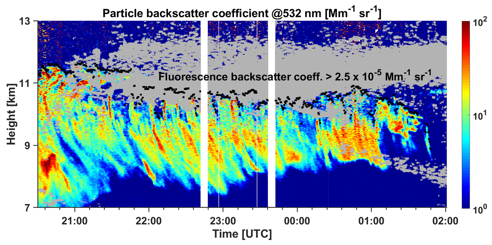
Figure 7 Height–time distributions of the particle backscatter coefficient at 532 nm in the night of 29–30 May 2023. Height–time bins with a high fluorescence backscatter coefficient (> 2.5 × 10⁻⁵ ${\mathrm{Mm}}^{-\mathrm{1}}{\mathrm{sr}}^{-\mathrm{1}}$) are colored in gray. The top of the ice cloud layer is marked in black.

In summary, our measurement results suggest two possible interaction pathways between the observed smoke layer and the cirrus clouds: fluorescence quenching and heterogeneous ice nucleation combined with aerosol scavenging. For further illustration, Fig. 7 shows the elastic and fluorescence backscatter coefficients together in one plot. The height–time bins with pronounced aerosol fluorescence (in gray color) along with the elastic backscattering at 532 nm clearly show major aerosol–cloud interplay. Just before 01:00 UTC, an interesting situation arose. The smoke particles were deeply embedded in the cloud, exhibiting two layers: one around 10 km and one between 8 and 9 km, accompanied by a significant increase in the elastic-backscatter coefficient.

A further potential application of fluorescence lidar is to provide INP information in such cases with a low but relevant aerosol presence in the cloud surroundings, especially at the cloud top. A conversion from the unambiguous fluorescence backscatter coefficient to an INP number concentration (N_INP) is desirable. An approach applying conversion factors, which link the fluorescence backscatter coefficient with the previously inverted microphysical properties of the fluorescing aerosol particles from multi-wavelength lidar data, was suggested by Veselovskii et al. (2022a). In the case of a low aerosol load or inside a cloud layer, the resulting mean conversion factors, together with the fluorescence backscatter coefficient, can then be used to derive the aerosol surface area concentration, which is needed as input to the INP parameterization (Veselovskii et al., 2022a). An alternative approach would be to determine N_INP directly from ice crystal number information provided by lidar–radar synergy and find a conversion factor between β_F and N_INP. Such a factor σ_F would be in the form of ${\mathit{\sigma }}_{\mathrm{F}}=N_{\text{INP}}/{\mathit{\beta }}_{\mathrm{F}}$ and could be used for cirrus cloud scenes with comparable temperature and humidity. Preliminary assessments of INP concentrations via the POLIPHON method (Ansmann et al., 2012, 2021) and ice crystal number concentrations from lidar–radar synergy (Bühl et al., 2019) suggest a conversion factor in the range of 3×10⁴–8 × 10⁴ Mm sr L⁻¹ at −50 °C.

A reliable conversion to link the fluorescence backscatter coefficient to ice nuclei concentrations would be beneficial to investigate aerosol–cloud interactions, especially in those situations with low aerosol amounts. Further aerosol–cloud cases will be investigated in the future to evaluate this potential application of fluorescence backscatter information specifically.

4 Conclusions

In this study, we present the newly implemented fluorescence channel in the lidar system MARTHA, located at TROPOS, Leipzig, Germany. Some of the first measurements performed with the upgraded system were during the summer wildfire season of 2023. The fluorescence capacity of wildfire smoke mainly ranged between 2 × 10⁻⁴ and 7 × 10⁻⁴, thus confirming previously reported values in the literature (Hu et al., 2022; Veselovskii et al., 2022a).

Special care was taken regarding the characterization of the fluorescence lidar, where each component along the optical path was considered in the determination of the system efficiency constants needed to derive the new fluorescence parameters. The detection of optically thin aerosol layers that are only recognizable in the fluorescence signal can significantly improve the detection capabilities of a lidar, which could be critical for low-particle-concentration situations. The enhanced sensitivity results from the fact that laser-induced fluorescence emission originates exclusively from aerosol particles, while air molecules and hydrometeors are excluded from this scattering process. Furthermore, as our observations showed, the new dedicated “particle” channel enables unambiguous differentiation between coexisting unactivated aerosol particles and hydrometeors within clouds.

Because of their strong fluorescence and rather low depolarization, the aerosol layers presented in the case studies could be identified as biomass-burning aerosol. The measurements showed that such optically thin smoke layers are not so rare in the UTLS region. This suggests that the atmosphere over Europe might be more polluted than previously thought, especially during the summer wildfire season. Those thin layers might not have a strong direct radiative impact, but at these altitudes, smoke particles could become an additional INP source in an otherwise relatively clean atmosphere. Investigating such aerosol layers with a fluorescence lidar, combined with advanced remote-sensing techniques to assess cloud microphysics, could provide more clarity about the relevance of heterogeneous freezing of smoke particles in cirrus cloud formation compared to homogeneous nucleation of background sulfate particles. Several observations of cirrus clouds directly below thin biomass-burning aerosol layers suggest that these might be the primary INP source, indicating that heterogeneous freezing is the dominant process. To thoroughly explore this potential aerosol–cloud effect, a larger data set would be beneficial and might provide stronger evidence and more detailed insights into this hypothesis.

Further instrumental upgrades are currently ongoing in the MARTHA system. A new powerful laser, together with a 32-channel spectrometer, will extend the observational sharpness and aim to provide state-of-the-art information about aerosol and clouds from the ground up to the stratosphere.