In situ vertical observations of the layered structure of air pollution in a continental high-latitude urban boundary layer during winter

Vertical in situ measurements of aerosols and trace gases were conducted in Fairbanks, Alaska, during winter 2022 as part of the Alaskan Layered Pollution and Chemical Analysis campaign (ALPACA). Using a tethered balloon, the study explores the dispersion of pollutants in the continental high-latitude stable boundary layer (SBL). Analysis of 24 flights revealed a stratified SBL structure with different pollution layers in the lowest tens of meters of the atmosphere, offering unprecedented detail. Surface emissions generally accumulated in a surface mixing layer (ML) extending to an average of 51 m, with a well-mixed sublayer (MsL) reaching 22 m. The height and concentrations within the ML were strongly influenced by a local wind driven by nearby topography under anticyclonic conditions. During strong radiative cooling, a drainage flow increased turbulence near the surface, altering the temperature profile and deepening the ML. Above the ML, pollution concentrations decreased but showed clear signs of freshly released anthropogenic emissions. Higher in the atmosphere, above elevated inversions, pollution levels were similar to previously reported Arctic haze concentrations, even though Fairbanks' outflow concentrations below elevated inversions were up to 6 times higher, likely due to power plant emissions. In situ measurements indicated that gas and particle tracer ratios in elevated power plant plumes differed significantly from those near the surface. Overall, pollution layers were strongly correlated with the temperature stratification and emission heights, emphasizing the need for improved representation of temperature inversions and emission sources in air quality models to enhance pollution forecasts.

1 Introduction

Air pollution in high-latitude urban areas during winter is a serious yet understudied issue (Schmale et al., 2018; Simpson et al., 2024; Tran and Mölders, 2011). Under extremely cold conditions, pollution emission rates from domestic heating and energy production are generally high, and traffic emissions at cold temperatures can release comparatively more pollutants than under higher temperatures due to inefficient combustion conditions (e.g., Brett et al., 2025; Weber et al., 2019; Zhu et al., 2022). Furthermore, the often very stable atmospheric conditions leading to a persistently stable boundary layer (SBL; for abbreviations see Appendix A) are characteristic of the wintertime high-latitude boundary layer and prevent an efficient vertical mixing of pollution (Cesler-Maloney et al., 2022; Malingowski et al., 2014; Salmond and McKendry, 2005). The combination of enhanced emission rates and weak dispersion leads to an accumulation of pollution at breathing level and health risks for the exposed population (e.g., ADEC, 2021; Lajili, 2019; Schwartz et al., 1996).

The winter in high-latitude continental regions is characterized by snow-covered surfaces with high longwave radiative emissivity combined with the quasi-absence of incoming shortwave radiation that together create a longwave radiation-dominated surface energy budget (Maillard et al., 2022; Mayfield and Fochesatto, 2013). Under anticyclonic conditions, with clear skies, the longwave upwelling radiation leads to a negative radiative energy budget at the surface (i.e., the surface loses heat). If the prevailing synoptic weather situation results in weak pressure gradients and hence low wind speeds, the very small turbulent heat flux cannot balance the surface energy loss, resulting in a cooling of the surface and the development of a surface-based inversion (SBI) and SBL (Bourne et al., 2010; Mahrt, 1999; Serreze et al., 1992; Stull, 1988). As long as the SBI persists and the surface keeps cooling, the turbulent heat flux towards the surface decreases even further as a result of increased static stability. This positive feedback can lead ultimately to a very stable boundary layer (VSBL), where turbulence collapses and becomes only intermittent (Steeneveld et al., 2006; Sun et al., 2012; Van de Wiel et al., 2012). Under these conditions, the air density gradient becomes strong enough to decouple the lower levels from the lower troposphere (Malingowski et al., 2014) and inhibits vertical mixing of surface pollutants.

In the high latitudes, a winter SBL can persist over several days (long-lived SBL) as opposed to the midlatitudes where a diurnal cycle typically prevails and the SBL is usually observed during the night (nocturnal boundary layer) or in regions without direct sunlight (Grachev et al., 2005; Stull, 1988). In the case of a diurnally varying SBL, the nocturnal boundary layer is often overlaid by a neutral layer (called the residual layer) that retains some of the pollution from the previous daytime thick convective mixed boundary layer. The residual layer separates the SBL from the free troposphere (FT). In contrast, a long-lived SBL is continuously in immediate contact with the FT (Zilitinkevich and Baklanov, 2002). However, the nature of the high-latitude winter lower atmosphere often presents a complex layered structure with several elevated temperature inversions (EIs) on the top of the SBI. Mayfield and Fochesatto (2013) investigated the wintertime temperature profile in Fairbanks, Alaska, using nearly 12 years of radiosonde data. Under SBL conditions, they found the frequent co-occurrence of stratified SBIs (i.e., SBIs with a layered structure) and EIs, which were generated either by large-scale subsidence or by warm air mass advection aloft. The SBI stratification is indicative of the surface cooling history and reflects potential differences in vertical diffusion of pollution within the SBL (Malingowski et al., 2014). EIs also act as additional barriers to the vertical dispersion of pollution. Hence, the vertical dispersion through the complex structure of northern high-latitude continental wintertime SBL is expected to be radically different from the dispersion within the well-mixed or short-lived stable boundary layers at midlatitudes. This means that conventional SBL descriptions from the literature (Mahrt, 1999; Mahrt and Vickers, 2002; Stull, 1988) may not be fully appropriate to explain the vertical distribution of pollution layers in the high-latitude winter SBL. This is partly due to the lack of detailed vertical measurements of air pollutants, especially in the long-lived high-latitude SBL (Berkowitz et al., 2000).

The vertical mixing in the VSBL is difficult to simulate in models because they often use the Monin–Obukhov similarity theory (MOST) with its assumed continuous turbulence and are therefore not able to correctly describe the very stable conditions of the high-latitude SBL (Lan et al., 2022). As a result, numerical weather prediction models frequently struggle to accurately simulate the VSBL, leading to significant forecast errors (Lan et al., 2022). VSBLs are also typically accompanied by strong SBIs, which are poorly simulated in current models (Maillard et al., 2024; Malingowski et al., 2014).

In winter 2022, the Alaskan Layered Pollution and Chemical Analysis (ALPACA) campaign took place in Fairbanks, Alaska (Simpson et al., 2024; Fochesatto et al., 2024). ALPACA aimed to improve understanding of chemical, microphysical and dynamic processes of air pollution in a very cold, dark and stable atmosphere. During winter, Fairbanks frequently experiences high-pollution episodes, when the concentration of particulate matter with diameters below 2.5 µm (PM_2.5) exceeds the U.S. Environmental Protection Agency (EPA) daily regulatory limit (35 µg m⁻³) (ADEC, 2021). Located about 800 km from the coast, with a “bowl-shaped” local topography, which partly shields the city from synoptic winds and favors accumulation of cold air at the bottom, Fairbanks experiences some of the strongest and longest-lasting SBIs in urban areas (Bourne et al., 2010; Tran and Mölders, 2011). SBIs in Fairbanks occur 82 % and 68 % of the days in January and February, respectively (Bourne et al., 2010). Tran and Mölders (2011) investigated the relationship between daily PM_2.5 concentrations, SBIs identified from radiosondes and various meteorological parameters. They found that PM_2.5 was highest during multiday SBIs with calm winds (< 1 m s⁻¹) and low temperatures (≤ −20 °C) as well as low moisture (water vapor pressure < 2 hPa). While this study confirmed the role of SBIs in high-pollution events at the surface, it did not directly investigate the effect on the vertical mixing and dispersion of pollution, when the SBL has a complex layered structure that was revealed by the Mayfield and Fochesatto (2013) study.

A key goal of ALPACA was to assess the impact of emissions (e.g., from traffic and domestic heating at the ground to power plant stacks with heights of 20 to 64 m above the ground) on pollution measured at different heights given the stratified character of the SBL. To fill in the observational gap of the vertical distribution of Fairbanks winter pollution, a tethered-balloon (Helikite) was deployed during the ALPACA campaign to carry out high-resolution in situ vertical measurements of air pollutants and meteorological variables. The Helikite was equipped with the Modular Multiplatform Compatible Air Measurement System (MoMuCAMS) (Pohorsky et al., 2024).

The aim of this study is to investigate the effects of surface and elevated emission sources on the vertical distribution of pollution in the SBL, based on the analysis of the balloon profile measurements and to understand how both synoptic and local meteorological conditions affect the mixing of local air pollution. Section 2 describes the methodology with details on the balloon site and measurements, as well as data processing and treatment of the vertically resolved data. Dynamic processes influencing the local boundary layer are described in Sect. 3. The observed layered structure of the lower atmosphere, notably the mixing layer height (MLH), is discussed in Sect. 4. The analysis of the layers' chemical composition is presented in Sect. 5. Finally, an analysis of elevated pollution plumes from power plants is presented in Sect. 6.

2 Measurements and analytical methods

2.1 Study site

Measurements of the vertical distribution of air pollution were performed at a study site in a suburban area, west of downtown Fairbanks (64°51^′12^′′ N, 147°51^′32^′′ W; 138 m above mean sea level). The site is located on a farm field near the University of Alaska (UAF) and will be referred to as the UAF farm site hereafter. Figure 1 indicates the location of the UAF farm site (red diamond) and the Community Technical College (CTC) site (yellow diamond), another ALPACA measurement site, located downtown focusing on surface-based gas and aerosol measurements. An overview of the campaign and different measurements sites is presented in Simpson et al. (2024). Figure 1 also indicates the location of power plants in Fairbanks (white triangles). The power plants emit particles and gases from tall stacks, which release emissions at higher altitudes. This elevated release height may lead to increased concentrations of pollutants in the upper portions of the boundary layer. As a result, the measured vertical profiles can reflect these elevated concentrations. The UAF power plant (Fig. 1a) had the most frequent influence on the vertical measurements due to its higher proximity, but plumes from the other power plants from Fig. 1 were also sampled on several occasions.

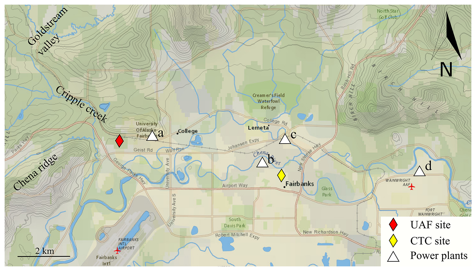
Figure 1 Map of Fairbanks, Alaska, USA. The red and yellow diamonds represent the location of the UAF farm and CTC study sites, respectively. White triangles indicate the location of the power plants in Fairbanks: (a) UAF power plant, (b) Aurora, (c) Zehnder and (d) Doyon (Fort Wainwright). The map was obtained and adapted from the United States Geological Survey (https://apps.nationalmap.gov/, last access: 26 March 2024).

The UAF farm site is characterized by a large and flat agricultural field covered in snow from roughly October to May. The field is bound by a small hill to the north and Chena Ridge to the west and is located at the exit of Cripple Creek and the Goldstream Valley to the northwest. An additional detailed map of the topography is presented in Fig. S1 in the Supplement. Because of this topography, the UAF farm site is under the influence of a drainage flow during periods of radiative cooling, where the cold air descending the neighboring hills is channeled through the Goldstream Valley and Cripple Creek. The drainage flow will henceforth be denoted as the shallow cold flow (SCF). The SCF and its influence on surface energy fluxes have been characterized by Fochesatto et al. (2015) and Maillard et al. (2022). We describe the effect of the SCF on the boundary layer structure in Sect. 3, and its influence on pollution mixing will be discussed in Sects. 4.1 and 5.1.

2.2 Measurements

2.2.1 Vertical in situ measurements from a tethered balloon

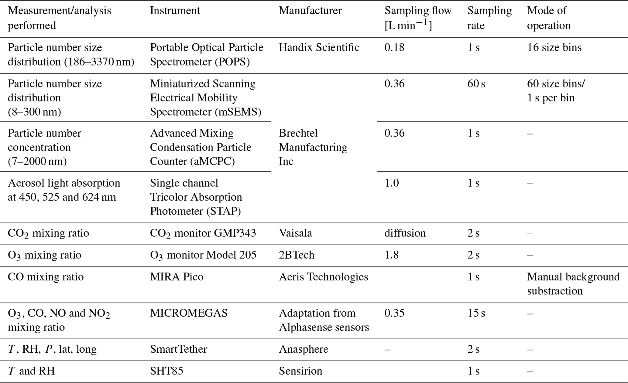
Vertical in situ measurements of atmospheric composition and thermodynamic variables were realized using an instrumental platform attached to a tethered balloon (45 m³, Desert Star, Allsopp Helikites Ltd., UK; Fig. 2). The Modular Multiplatform Compatible Air Measurement System (MoMuCAMS), previously described in Pohorsky et al. (2024), was equipped with various instruments and sensors to measure aerosol properties, various trace gases and meteorological variables: particle number size distributions (PNSDs) with concentrations from the optical (186–3370 nm) and electrical mobility (8–270 nm) spectrometers; aerosol light absorption coefficients at 450, 525 and 624 nm; and CO, CO₂ and O₃ mixing ratios. An additional trace gas package (MICROMEGAS) also provided O₃, CO, NO and NO₂ data from electrochemical sensors. Details on the MICROMEGAS package and specifics on data processing and validation are described in Barret et al. (2025). Meteorological variables included temperature, pressure and relative humidity. A detailed list of the measured variables and respective instruments is given in Table 1; sampling efficiencies, measurement uncertainties and limits of detection are discussed in detail in Pohorsky et al. (2024). Note that concentrations in Fairbanks were always well above detection limits.

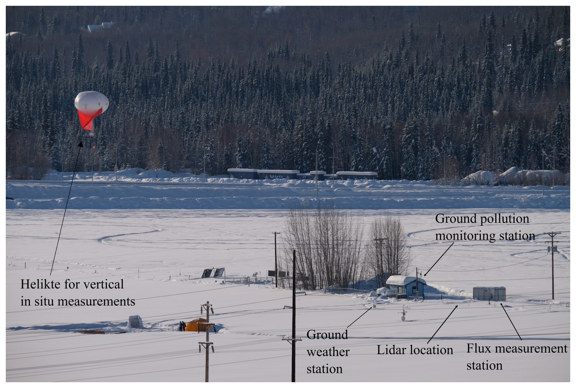
Figure 2 Photo of the UAF farm study site with the different infrastructures for ground-based and vertical measurements.

Table 1 List of measurements performed with the Helikite and their respective instruments and operation details.

Data for each flight were manually time-synchronized using pressure readings from each instrument. A visual check of each flight for quality control was done to remove spurious data and spikes. The altitude was calculated using the barometric formula as described in Pohorsky et al. (2024).

The raw light absorption coefficients (b_abs) from a single-channel tricolor absorption photometer (STAP) were corrected for filter loading and increased scattering of particles deposited on the filter using the routine provided by the manufacturer. Equivalent black carbon (eBC) mass concentration was calculated from light absorption coefficients, using

$$\begin{array}{}\text{(1)}& \text{eBC}={\displaystyle \frac{b_{\mathrm{abs}}\left(\mathit{\lambda }\right)}{\text{MAC}\left(\mathit{\lambda }\right)}},\end{array}$$

where MAC is the mass absorption cross-section. Typically, eBC is calculated at 880 nm (Ramachandran and Rajesh, 2007). Since the longest wavelength of the STAP is 624 nm, the MAC value for this wavelength was calculated using

$$\begin{array}{}\text{(2)}& \text{MAC}\left(\mathit{\lambda }\right)=\text{MAC}\left(\mathrm{550}\right){\left({\displaystyle \frac{\mathit{\lambda }}{\mathrm{550}}}\right)}^{-\mathrm{AAE}},\end{array}$$

where AAE is the absorption Ångström exponent (Li and May, 2022) and λ = 624 nm. The MAC value (at 550 nm) of 7.5 m² g⁻¹ was used based on the review of laboratory studies from Bond and Bergstrom (2006). The AAE was calculated at each time step using the most distant wavelengths of the STAP (450 and 624 nm):

$$\begin{array}{}\text{(3)}& {\text{AAE}}_{\mathrm{450}/\mathrm{624}}=-{\displaystyle \frac{\ln \left(\frac{b_{\mathrm{abs}}\left(\mathrm{450}\mathrm{nm}\right)}{b_{\mathrm{abs}}\left(\mathrm{624}\mathrm{nm}\right)}\right)}{\ln \left(\frac{\mathrm{450}}{\mathrm{624}}\right)}}.\end{array}$$

The performance of the STAP was previously reported by Bates et al. (2013), Pikridas et al. (2019) and Pilz et al. (2022), and b_abs showed good agreement with other filter-based reference instruments such as the multiangle absorption photometer (MAAP). Note that the determination of the eBC concentration highly depends on the appropriate quantification of the MAC value. Here we followed a theoretical procedure (cf. Eqs. 2 and 3) based on values obtained from laboratory studies in the absence of direct elemental carbon measurements, yielding MAC values between 6.3 and 6.6 m² g⁻¹ at 624 nm, which is close to the nominal value of 6.6 m² g⁻¹ at 637 nm of the MAAP. These relatively low values can however lead to an overestimation of the eBC mass concentration as suggested by the study of Savadkoohi et al. (2024), which reported that local MAC values for the MAAP were typically higher than the nominal value of the instrument (10.6 ± 4.7 m² g⁻¹). In the absence of comparison with direct elemental carbon measurements, the reader should keep in mind the range of MAC values used to derive eBC in this study.

The raw CO₂ data were corrected to a standard pressure (1013 hPa), and a calibration correction factor (CO_2,corr = $\mathrm{1.01}\times {\mathrm{CO}}_{\mathrm{2},\mathrm{raw}}-\mathrm{26.3}$) from laboratory comparisons with reference air mixtures (400 and 800 µmol mol⁻¹ of CO₂) was applied. The instrument automatically corrects the data for temperature with a built-in temperature sensor.

The CO data were corrected by removing the instrument's measured baseline (CO value measured when sampling from a CO scrubber; see Pohorsky et al., 2024). The baseline was evaluated for a 30 min period before and after each flight. A linear interpolation of this baseline was applied to account for changes between the beginning and the end of the flight. The baseline was subtracted from the raw measurements of CO. All raw CO measurements are directly converted to standard temperature and pressure (0 °C and 1013 hPa) by the instrument. All aerosol concentrations were converted to standard temperature and pressure (0 °C and 1013 hPa).

For the analysis of vertical profiles, the in situ data from the Helikite were spatially averaged in 2 m vertical bins, except for the PNSD (8–270 nm) data from the miniaturized scanning electrical mobility sizer (mSEMS) and the trace gas data (CO and NO_x) from the MICROMEGAS package (Barret et al., 2025). Since the time resolution of the mSEMS is coarser than the other instruments on MoMuCAMS (1 min; see Table 1), the spatial resolution of the PNSD from 8 to 270 nm exceeds 2 m and highly depends on the traveling speed of the Helikite (i.e., ascending or descending rate). The coarser spatial resolution for a 20 m min⁻¹ vertical speed (maximum speed of the winch) is 20 m. The mSEMS data were therefore kept at their original resolution without any further averaging. The data from the electrochemical trace gas package (MICROMEGAS) were processed separately with 15 s time averaging (see Barret et al., 2025).

From 26 January to 25 February 2022, 24 flights were performed with MoMuCAMS (see Table S1 in the Supplement for details). Since the maximum altitude of daytime flights (∼ 120 m) was about 3 times lower than the one of nighttime flights (∼ 350 m) due to airspace restrictions, more but shorter profiles (i.e., full ascents and descents of the balloon) could be carried out during daytime flights, i.e., typically between 8 and 14 (ascents and descents counted separately). For night flights, between two and six profiles were performed. Flight patterns usually consisted of a rapid ascent (∼ 20 m min⁻¹) to obtain a snapshot of the atmospheric vertical profile followed by a stepwise descent with roughly 10 min hovering stops to obtain better counting statistics from the instruments at different altitudes. Details on the spatial resolution and sampling for a specific flight pattern are provided in Pohorsky et al. (2024). On several occasions, when an elevated pollution plume was detected, the Helikite hovered at the plume altitude for an extended period to maximize data collection. In total, 148 individual profiles were collected with varying instrumental setups.

2.2.2 Additional measurements

In addition to the in situ vertical measurements, a series of ground-based measurements provided continuous surface pollution and meteorological data, as well as turbulence observations and vertical information on wind speed and direction from remote sensing. Figure 2 shows the overall setup of the UAF farm site, and further details are given in Fochesatto et al. (2024).

Surface pollution measurements

Aerosol number concentrations and size distributions were continuously measured from a hut located roughly 50 m from the Helikite launch and landing site. A heated, 1.8 m long stainless-steel aerosol sampling line (8 mm inner diameter) sampled total suspended particles (no cut-off diameter). The nominal flow rate was 3.48 L min⁻¹ (liters per minute). The inlet was equipped with a custom-made silica gel column (similar to a TSI 3062 model) to ensure relative humidity below 40 % according to the Global Atmosphere Watch aerosol measurement recommendations. Behind the dryer, the sampled air was distributed to the different instruments through an isokinetic flow splitter. Conductive silicon tubing was used to connect the different branches of the flow splitter to the instruments. Instruments were placed to minimize the tubing length (∼ 60 cm on average) and bends. Losses in the inlet were characterized using the Particle Loss Calculator (PLC) (von der Weiden et al., 2009). Figure S2 shows the results of the calculated transmission efficiency in the inlet. The transmission efficiency was above 90 % within our measurement size range. The PNSD data were corrected for particles losses. The gas sampling line was installed adjacent to the aerosol inlet and made of Teflon tubing.

The aerosol number concentration above 7 nm was measured using an advanced mixing condensation particle counter (aMCPC model 9403, Brechtel Manufacturing Inc., USA). The size distribution from 8 to 1500 nm was measured with a scanning electrical mobility spectrometer (SEMS model 2100, Brechtel Manufacturing Inc., USA). An optical particle counter (POPS, Handix Scientific, USA) provided an extended size distribution measurement from 186 to 3370 nm. In addition, between flights, all instruments from the MoMuCAMS were connected to the main inlet in the hut, providing semicontinuous measurements of aerosol light absorption, CO and O₃.

The ground-based aerosol and trace gas raw data were corrected for local pollution emissions. Concentration spikes from nearby idling cars or snowmobiles were removed based on campaign notes. Remaining spurious pollution spikes in the measured time series were filtered out with a “despiking” function. To do so, we calculated a 5 min running median of the measured time series, hereafter called the “reference” time series. The standard deviation of the difference between the measured time series and the reference was then calculated, and data points that deviated from the reference by more than 3 times the standard deviation were eliminated.

Finally, the data were corrected to standard temperature and pressure and averaged using a 5 min arithmetic mean. All ground-based instruments have been compared to the MoMuCAMS instruments to ensure comparability between flight and ground data (Pohorsky et al., 2024).

Meteorological measurements

Meteorological measurements were performed with a weather station installed above the snow surface. The temperature and relative humidity sensor (HygroVUE10, Campbell Scientific, UK) was placed at a height of 2 m. The wind probe (Heavy Duty Wind monitor-HD-Alpine, R. M. Young, USA) and the four-component radiation sensor (SN-500, Apogee Instruments Inc., USA) were placed at 3 m. The data were recorded at 5 min averaged intervals.

Eddy covariance measurements

A turbulence measurement system was located at the top of an 11 m pneumatic mast next to the hut (Fochesatto et al., 2024). Specifically, the eddy covariance station included an ultrasonic anemometer (R3-100; Gill Instruments Limited, UK) with a 100 Hz acquisition frequency to measure wind velocity and direction. Air temperature and relative humidity were measured at the same height by a conventional thermo-hygrometer (model XD33A-W3X, Rotronic, Switzerland). The setup was the same as in Donateo et al. (2023). A 30 min arithmetic mean was used to average the turbulence and flux data to reduce measurement errors and increase statistical significance. To avoid the influence of slow submesoscale atmospheric motions, a digital filter was applied to the dataset according to Pappaccogli et al. (2022). The turbulence measurements were used to calculate the Obukhov length (L), the friction velocity (u_∗) and the buoyancy flux (Bs).

Lidar

Wind speed and direction measurements were performed with a Doppler wind lidar (WindCube v2; Vaisala, Saclay, France) installed on the ground next to the eddy covariance station. The lidar was installed at the UAF farm site on 8 February 2022. Prior to that date, the lidar operated at the CTC site downtown (Fig. 1). The lidar employs the Doppler beam swinging method to capture three wind components, utilizing a combination of five beams: four directed north, south, east and west at a 62° elevation angle from the ground, along with one vertical beam. Each beam had an accumulation time of 1 s, resulting in a wind profile retrieval every 5 s, with a precision of 0.1 m s⁻¹. These wind profiles were subsequently averaged over 10 min intervals. Wind data were collected at 20 m intervals from 40 to 300 m above the instrument. More details on the lidar data can be found in Dieudonné et al. (2023), Simpson et al. (2024) and Brett et al. (2025).

2.3 Comparability between vertical and ground-based measurements

To assess the comparability of measurements conducted with the MoMuCAMS system with those obtained at the ground, data measured below 2 m for each profile were averaged and compared to simultaneous measurements from the blue hut or the weather station. Figure S3 presents the results for number concentrations measured using (a) the POPS (N_186−3370) and (b) the SEMS and mSEMS (N₈₋₂₇₀). Figure S3c shows the comparison of temperature measurements. The measurements demonstrate excellent agreement, with regression slopes of 0.92, 0.90 and 0.98, respectively. The coefficients of determination (R²) equal 0.95, 0.97 and 0.99, respectively. Since aerosol light absorption coefficients, as well as CO and O₃ mixing ratio measurements, were not duplicated on the ground during the flights, direct comparisons were not possible.

2.4 Temperature profile analysis method

The wintertime atmospheric boundary layer of Interior Alaska often exhibits a complex stratified structure with multiple layers (Mayfield and Fochesatto, 2013). Here, we refer to “layers” as vertical portions of the atmosphere with specific thermodynamic properties (e.g., same temperature gradient). To identify the different layers in the measured temperature profiles, the layer detection algorithm from Fochesatto (2015) was adapted to measurements from our Helikite profiles, which have a higher vertical spatial resolution compared to radiosonde observations (due to the slower ascending or descending rate of the tethered balloon) but with a much lower maximum altitude. The algorithm extracts the temperature inflections through a linear interpolation function of variable length that minimizes an error function between the observed data and the fit. “Inflections” are defined as changes in the absolute value of the temperature gradient that are significant enough to be detected by the algorithm. In its original version, the error function was defined as follows:

$$\begin{array}{}\text{(4)}& \mathit{\epsilon }=\Vert \mathrm{\Phi }\left(z\right)-T\left(z\right)\Vert ,\end{array}$$

where ε represents the Euclidian distance between the linear piecewise representation of the temperature profile Φ(z) and the observed temperature T(z) at height z. Since ε depends on the spatial resolution of the measurements, we modified the error function into an integral form as follows:

$$\begin{array}{}\text{(5)}& \mathit{\epsilon }={\int }_{\mathrm{b}}^{\mathrm{t}}\left(\mathrm{\Phi }\left(z\right)-T\left(z\right)\right)\mathrm{d}z,\end{array}$$

where indices b and t represent the bottom and the top altitude of the evaluated profile layer.

For the analysis, the temperature data were smoothed with a Gaussian running filter over 10 m. The ε threshold was set to 0.8 °C per layer Δz based on visual examination of the resulting simplified profiles that confirmed that the major temperature inflection points were correctly captured by the adapted algorithm. The physical meaning of this threshold was not further investigated as turbulence observations were lacking, and the aim was primarily the identification of temperature inversions, their depth and mean temperature gradient. As in Fochesatto et al. (2015), the relationship between the threshold ε, the captured temperature gradient dT dz⁻¹ and the overall final error is not straightforward and depends on the thickness of the layer. From the analyzed profiles, the temperature gradient difference between all pairs of adjacent layers had a median of 4.0 °C per 100 m with an interquartile range from 1.6 to 7.4 °C per 100 m. The lowest difference between two layers was 0.12 °C per 100 m.

Figure 3 shows examples of two temperature profiles measured on separate flights. The black lines represent the smoothed data, and the red lines represent the simplified profile from the algorithm, with red dots indicating the temperature profile inflection points. Both profiles show an SBI but with a different structure. Figure 3a shows one inflection point just above 100 m. The temperature gradient is the strongest below the inflection point (directly from the surface) and decreases above the inflection point but remains positive. This second layer illustrates the stratification of temperature inversions (stratified surface-based inversion, SSBI) as observed previously by Mayfield and Fochesatto (2013). In this specific case, the altitude where the temperature gradient reverses its sign (i.e., SBI top) is not known because it was above the flight's maximum altitude. Figure 3b shows a first inflection point at 40 m, which marks the bottom of a stratified layer with a higher temperature gradient (22.7 °C per 100 m) than the lowermost layer, and a second inflection point at 67 m, where the temperature gradient sign reverses from positive to negative (top of the SBI). The temperature gradient becomes positive again above 175 m; however, given the weakness of the gradient and the maximum vertical extent of the flight, it is not possible to tell whether this represents an elevated inversion (EI). The main difference in Fig. 3b compared to Fig. 3a is that the strongest temperature inversion layer is not located directly at the ground but some meters above it. Hereafter, SBIs with a structure similar to Fig. 3a are referred to as “convex” SBIs, while the shape described in Fig. 3b will be referred to as an “S-shaped” SBIs. These SBI regimes resemble observations made by Vignon et al. (2017) at Dome C in Antarctica, where very stable and weakly stable boundary layer conditions were associated with a convex SBI and convex–concave–convex (here S-shaped) SBI, respectively. The relation between the SBI shape, the radiation budget and surface wind speed is discussed in Sect. 3.

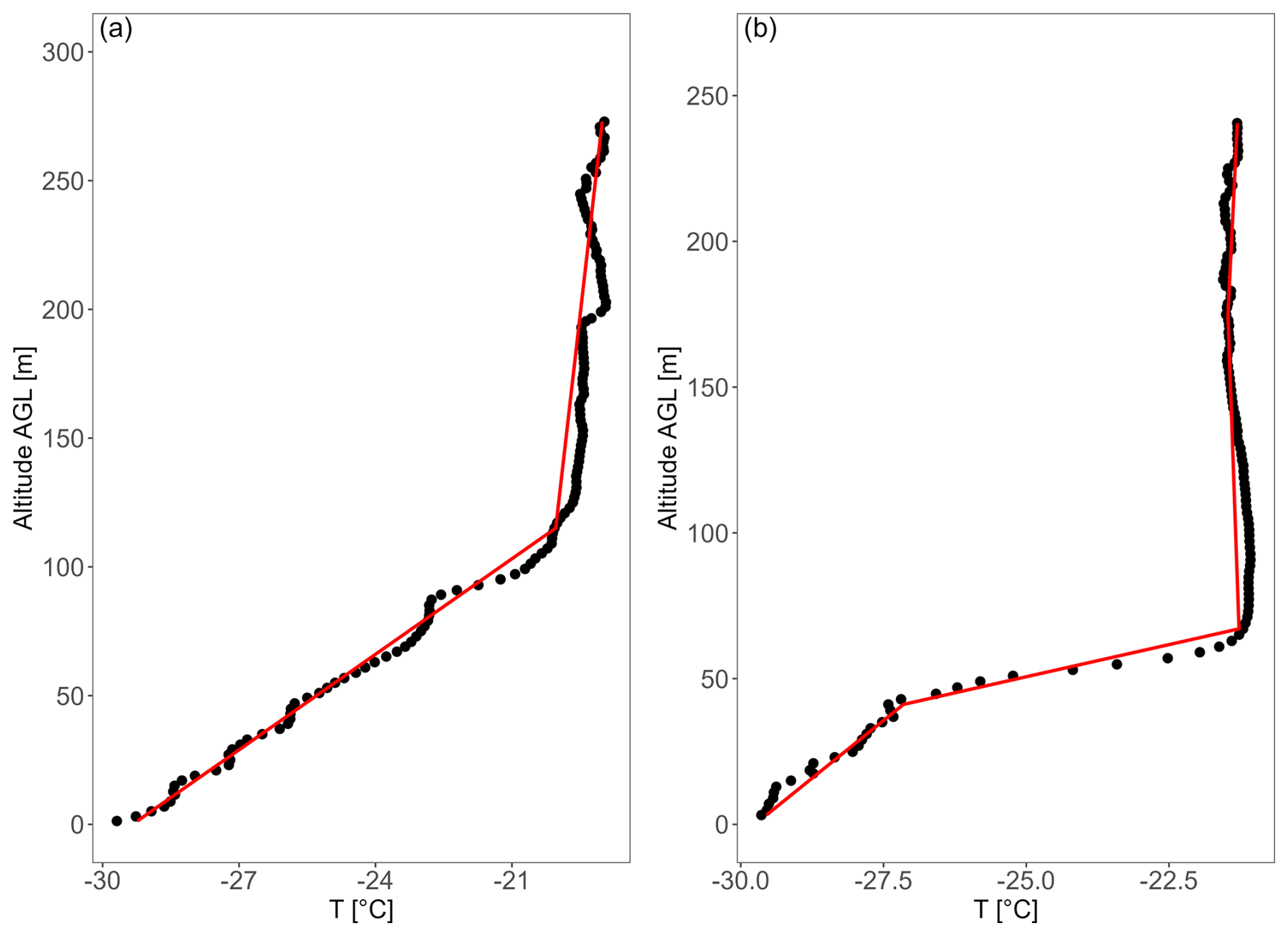
Figure 3 Vertical temperature profiles measured on (a) 31 January (flight 6) and (b) 10 February 2022 (flight 16). Black lines represent observations from the Helikite smoothed with a Gaussian filter. Red lines represent the simplified profile from the Fochesatto (2015) layer analysis algorithm, and red dots show the location of the inflection points.

The method was applied to all profiles to identify cases with an SBI and extract statistics on their height (m), strength (°C m⁻¹) and stratification structure (convex or S-shaped), which are later compared to vertical concentration profiles of different atmospheric composition tracers.

3 Synoptic- and local-scale processes influencing boundary layer properties at the UAF farm site

When an SBI develops, a fragile radiative equilibrium exists between the upwelling longwave radiation from the surface and the downwelling longwave radiation from aloft (Mayfield and Fochesatto, 2013). It can however easily be disrupted if the longwave downwelling increases (e.g., from the presence of low-level clouds) or if surface winds develop, which would alter the stratification of the temperature profile and consequently affect pollution trapping near the surface. Here, we investigate how synoptic and local processes influence the structure of SBIs at the UAF farm site during the campaign. Figure 4 shows the two-dimensional kernel density of measurements at 2 m height, which illustrates the relationship between the total surface radiative balance and the strength of the SCF with the measured surface wind speed as a metric. The different dots indicate Helikite profiles, and their color represents the surface pressure. A bimodal pattern emerges where cyclonic conditions are associated with lower pressure, a less negative radiation budget (> −25 W m⁻²) and lower surface wind speeds, while anticyclonic conditions are associated with a radiation balance between −25 and −50 W m⁻² and surface wind speeds typically above 2 m s⁻¹. Note that flight no. 16 (10 February; top right in Fig. 4) is an exception as it occurred during a transition period, during which a cloud was advected and reduced the surface radiative cooling, while the inertia of the SCF maintained higher wind speed at the surface during the flight. This bimodal pattern for this site was previously described in Maillard et al. (2022), who showed that the vertical turbulent sensible heat flux during the cyclonic mode was close to 0 W m⁻², due to lower wind speeds and a weaker vertical potential temperature gradient, and around 15 W m⁻² during anticyclonic periods, due to increased mixing from the stronger SCF.

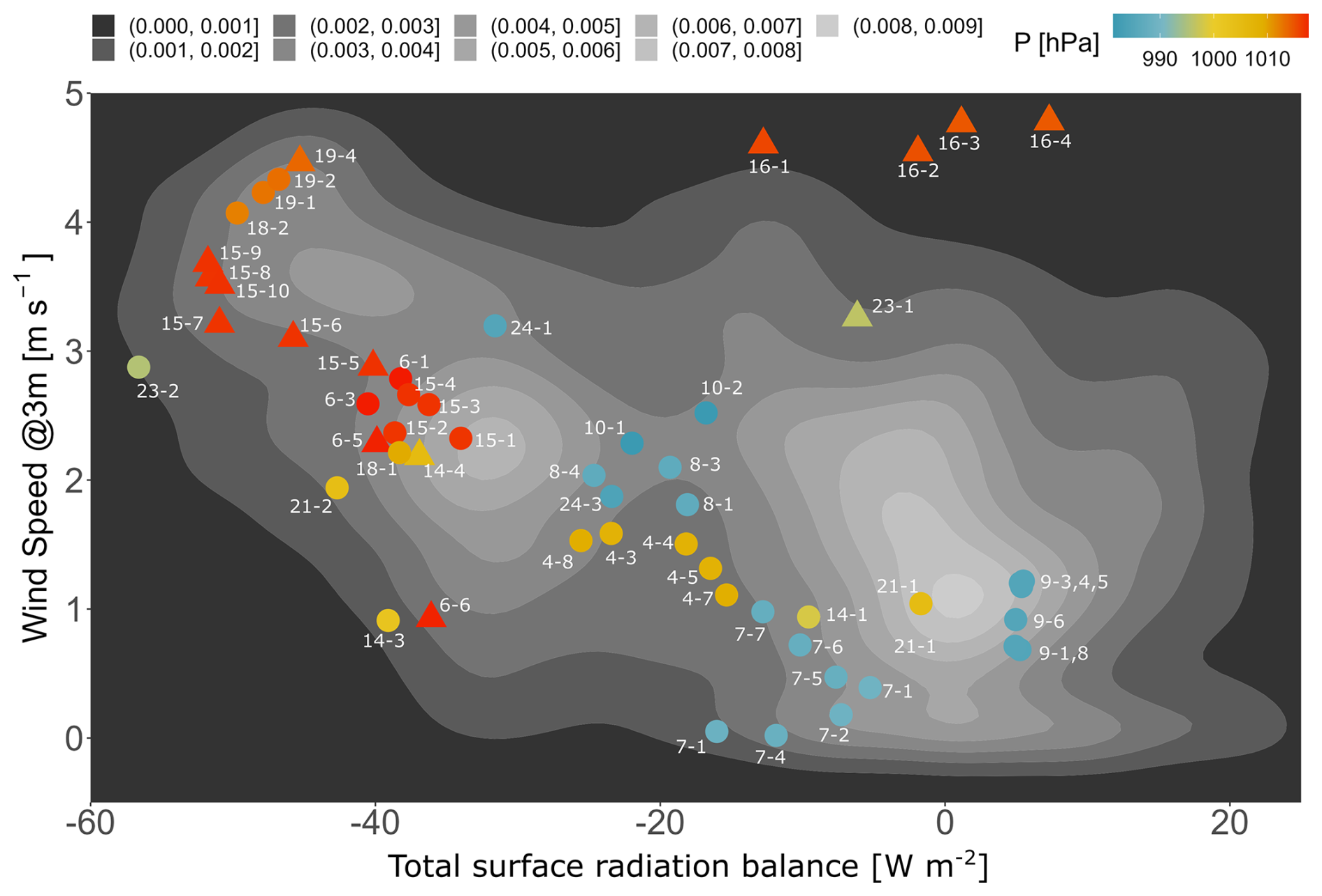
Figure 4 Gaussian kernel density plot (grey shading) of wind speed at 3 m (m s⁻¹) versus the total radiation balance (W m⁻²). Dots represent each flight profile (with available temperature data). White numbers indicate the flight and profile number, respectively. The color of the dot indicates the measured surface pressure during the profile. Round markers indicate profiles with a convex SBI as in Fig. 3a. Triangles indicate profiles with an S-shaped SBI, as illustrated in Fig. 3b.

With regards to the SBI during flights, we observe more cases of S-shaped SBIs with a reduced temperature gradient near the surface (as in Fig. 3b) when the strength of the SCF increases (triangles in Fig. 4). Under increased radiative cooling, the surface energy demand will typically exceed the downward heat flux eventually, resulting in further increase of the positive temperature gradient (Lan et al., 2022), leading to a stronger inversion and VSBL. However, our observations point to a competing effect during clear-sky conditions. Although the thermal energy loss at the surface increases the static stability, the increased surface wind speed caused by the SCF tends to increase mechanical turbulence development from the shear stress at the surface (Maillard et al., 2022). The combination of these effects increases the vertical heat flux near the surface, leading to a more homogenous cooling of the entire atmospheric surface layer, below the first inflection point of the S-shaped SBI situation (Fig. 3b). This process invokes a transition to a weakly stable boundary layer as described by Van de Wiel et al. (2017). This weakly stable layer is however limited to roughly 30–40 m (Table 2). Because the effect of surface friction decreases with height, a very stable capping layer develops above the surface layer at 30–40 m height, resulting from the positive feedback mechanism under strong radiative cooling and low shear stress. Flight no. 15 illustrates this mechanism (see Fig. S4, where the S-shaped structure develops from the first to the last profile). Overall, this transition when surface wind speed increased during Helikite profiling was observed on three flights. This interplay between radiative cooling and the SCF has an effect on atmospheric pollutant mixing and is addressed in Sect. 5. Note that the effect of the SCF appears to be localized, and the SBI profile in the larger Fairbanks area, when radiative cooling is strong, might be of the convex type. The shallow cold-flow influence rarely extends beyond the exit of the Goldstream Valley because towards Fairbanks the topography opens to a wider plateau and the urban canopy interferes with the SCF.

Table 2 Summary of flights with a surface-based inversion and associated general synoptic conditions. The indicated values are for the flight-averaged temperature profile. For S-shaped SBIs, values for the first two temperature layers are indicated.

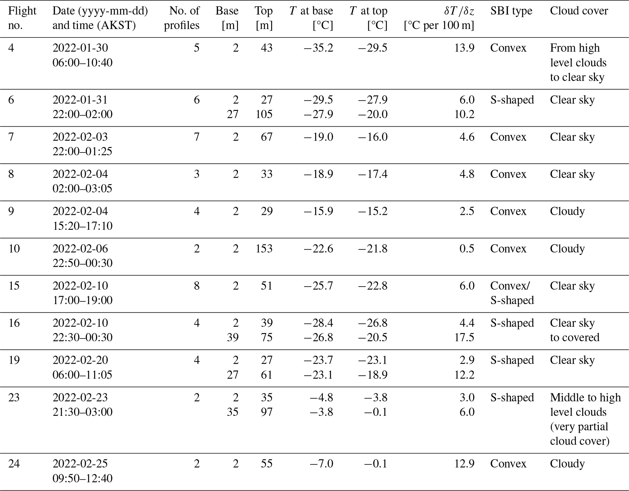
Of all analyzed flights ($\mathrm{21}/\mathrm{24}$ flights), 71 % ($\mathrm{15}/\mathrm{21}$ flights) showed at least one profile with an SBI. For the three flights not analyzed, the temperature sensor malfunctioned, and the data were either not recorded or discarded. Of the 15 flights, the SBI persisted for the full flight period (from 2 to 5 h) for 13 flights (60 %). Two of the 13 flights (dedicated to filter-based aerosol sampling, not discussed in detail here) carried a different instrumental payload and are therefore not included in the analysis presented below. Hence, 11 flights were retained to analyze the relation between the atmospheric conditions and the vertical distribution of pollution. A summary of the flight-averaged SBI parameters of these flights is listed in Table 2. For cases of convex SBIs (observed in seven flights), the temperature gradient ranged from 0.5 to 14.6 °C per 100 m for individual profiles. The large difference in the observed temperature gradients is related to the total surface radiative balance. For most cases of the convex SBI, the total radiative balance ranges from roughly −25 to 5 W m⁻². S-shaped SBIs typically occur under clear skies as indicated above (observed in five flights). Although some clouds were observed in individual cases, they were generally dispersed (i.e., partial sky coverage) high-level clouds. The gradients in the first atmospheric layer (i.e., closest to the ground) ranged from 0.5 to 6.32 °C per 100 m, and in the capping layer, they ranged from 7.2 to 27.2 °C per 100 m.

In Sects. 4.1 and 5 the vertical extents of surface pollutants' mixing and their concentrations are analyzed and compared for these different cases of SBL structure.

4 Defining the complex layering of the lowermost atmosphere in Fairbanks

Because of the complex boundary layer structure of wintertime central Alaska, we introduce here a simplified representation illustrating the main features observed from the measured vertical profiles for long-lived SBL at the UAF farm site. Figure 5 shows a temperature profile (solid and dashed blue line) with the two types of observed SBIs (Fig. 3), which usually present a layered structure. One or several EIs are also often observed. These EIs are usually decoupled from surface processes and originate either from warm air mass advection aloft or adiabatic warming from subsiding air (Mayfield and Fochesatto, 2013). The red line in Fig. 5 represents the pollution concentration profile, as generally observed in the lowest part of the atmosphere by the Helikite (up to 350 m), and the dashed line shows some of the possible variations. This profile is typically valid for the observed pollutants (aerosol particle microphysics, eBC, CO, CO₂ and NO_x), while the ozone profile typically shows an opposite trend (see Sect. 5). Starting from the bottom, a shallow layer with a rather homogeneously mixed profile is present. Here, this first layer is referred to as the mixed sublayer (MsL), with a concentration gradient near zero (dC dz⁻¹ ∼ 0), and represents a part of the overall mixing layer (ML). The term “mixing” refers here to the ongoing process and is used to indicate that complete mixing is not achieved in the SBL (Seibert et al., 2000). Above the MsL, the pollution concentration decreases (dC dz⁻¹ < 0) and reaches a background value, where the concentration gradient approaches a value near zero again (dC dz⁻¹ ∼ 0), marking the top of the ML. Note that in certain situations, no MsL is observed, and the concentration gradient is strongly negative directly from the surface (dashed lines in Fig. 5). These observations of the ML structure are similar to observations of SO₂ mixing ratios with a long-path differential optical absorption spectrometer performed at the CTC measurement site downtown (Cesler-Maloney et al., 2024). This method differs from methods that use the maximum absolute gradient or the second derivative to identify the MLH. Given that multiple layers were frequently observed or strong gradients occurred close to the surface, an automatic detection method based on the strongest concentration gradient is not applicable in the observed profiles.

Above the ML, the pollution is typically much lower and homogeneously distributed. The observed concentrations are however typically higher than a clean sub-Arctic background, depending on the main wind direction (see discussion in Sect. 5.2). This weak pollution signature is likely the combination of elevated pollution sources (e.g., power plant emissions or hillside residential emissions), mixing events due to SBI erosion and potential upward pollution fluxes from the SBL. This background pollution is trapped below the EI. To distinguish this layer from a cleaner sub-Arctic air background, we call it the weakly polluted background layer (WPBL). Here, we distinguish the WPBL from a residual layer (typically observed above the nocturnal boundary layer) because of the possible long-lived nature of the observed SBL. The observed pollution signature is therefore not necessarily a residual of a well-mixed boundary layer. Since, our observations do not provide a historic context of the boundary layer development, it is not necessarily possible to define whether the WPBL corresponds to the residual of a previous higher mixing layer (i.e., classic residual layer) or whether it is the result of direct emissions above the ML. Hence, the WPBL is used here as a generic term to describe the layer located between the ML and the clean background.

The layer observed above the EI is referred to as the lowest (meaning low concentration values) background layer (LBL). Given the limited vertical extent of the Helikite flights during the campaign (max 350 m), it was not possible to establish with full certainty whether the observed concentrations above the EI were representative of a true free-tropospheric background. Pollution levels in the different layers we observed are discussed and compared to the literature in Sect. 5.

In addition to the described structure, narrow plumes of highly enhanced pollutant concentrations were observed aloft when the wind was from the east. These elevated plumes are generally attributed to power plant emissions from high stacks with more elevated injection heights compared to residential heating or traffic emissions (see Brett et al., 2025). Plumes have been observed both in the WPBL where they were capped below an EI and above an EI.

The vertical extents of the MsL and ML are discussed in Sect. 4.1, and the concentration and composition of the different layers are discussed in Sect. 5. An analysis of elevated plumes is presented in Sect. 6.

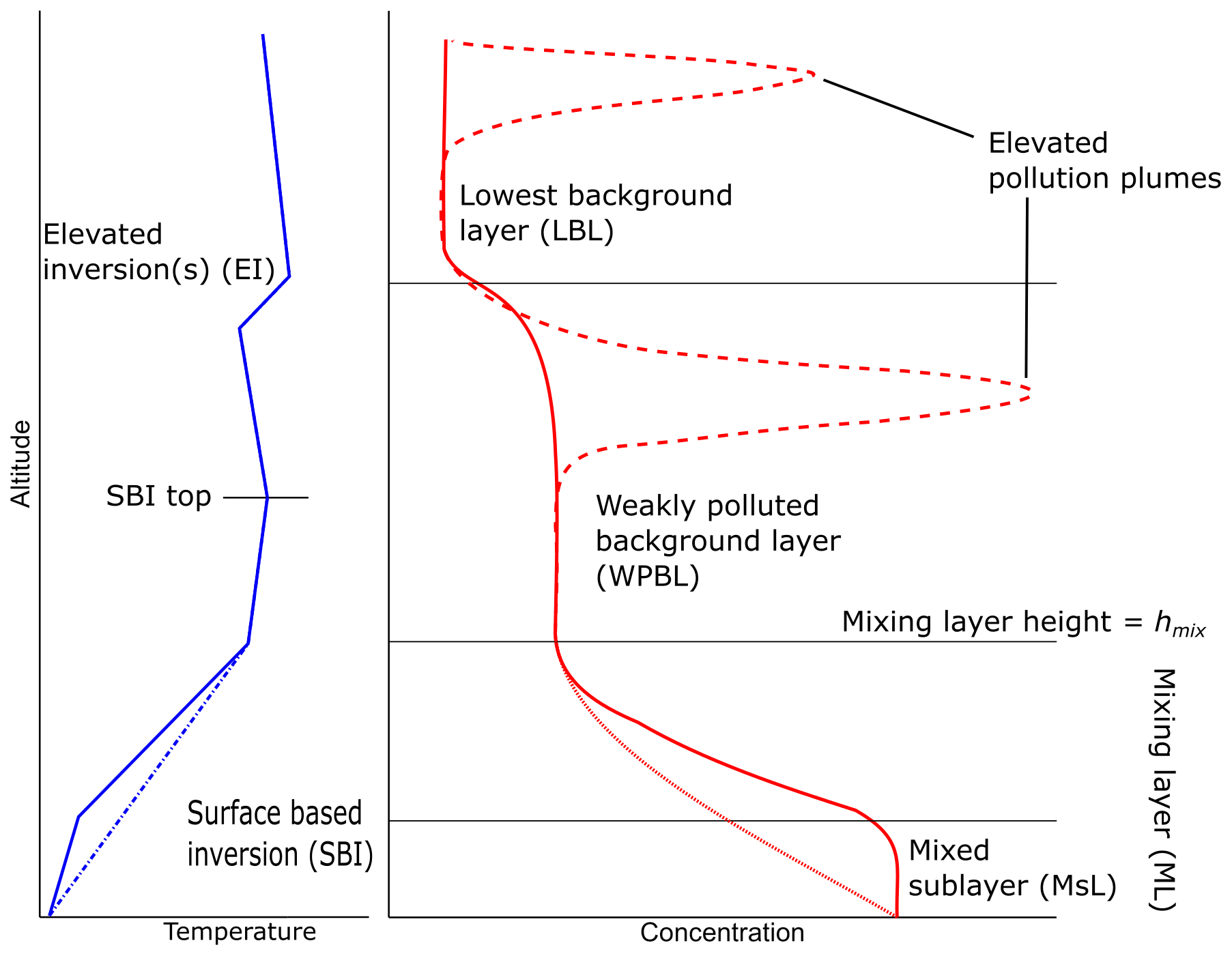
Figure 5 Schematic illustration of profiles observed in suburban Fairbanks during stable boundary layer conditions. The solid red line illustrates the concentration profile of a generic pollution tracer. The various dashed lines show observed alternative profiles.

4.1 Mixing layer height in the stable boundary layer

A key aspect of surface pollution in SBL conditions is the height of the ML, an essential parameter driving pollution levels at breathing height. In models that use a vertical prescription of the diffusion coefficient (K_z), an explicit formulation for the MLH is required to model the vertical diffusion of pollutants (Steeneveld et al., 2007; Vickers and Mahrt, 2004). However, mixing in the SBL is typically slower than in the convective BL, and a fully mixed SBL is typically not observed (Nieustadt, 1984; Seibert et al., 2000). Here, we use direct observations of altitude-resolved pollution tracer's concentrations to evaluate the MLH in the SBL. The MLH is defined here as the height where the pollution concentration reaches values in the WPBL. We describe how the MLH was determined and show the characteristics from flights in stable boundary layer conditions. The height was visually evaluated for each available air tracer on each profile and averaged to obtain the best estimate. The visually determined MLH is called h_mix hereafter.

Figure 6 shows examples of profiles to illustrate the methodology. The left panels (a, e, i) show the measured temperature profile (black dots) and the simplified profile from the Fochesatto (2015) algorithm in red (cf. Sect. 2.3). The other columns show selected air tracers, i.e., the particle number concentration, the geometric standard deviation (σ_geom, dimensionless) of the particle number size distribution between 8 and 270 nm (see Sect. 5.3 for a discussion on the PNSD in different layers), and the CO₂ mixing ratio. The horizontal blue line represents h_mix. Note that the particle number concentration from 7 nm and CO and O₃ mixing ratios were also used when available for the overall determination of h_mix.

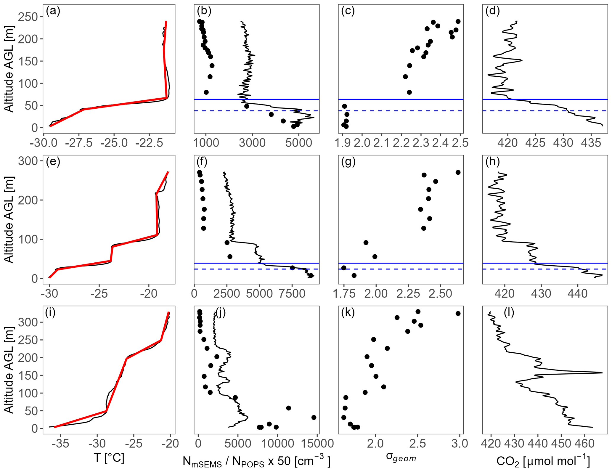
Figure 6 Examples of the atmospheric layered structure for three different profiles. (a, e, i) Temperature profiles. The red line represents the simplified profile obtained from the Fochesatto (2015) temperature analysis algorithm. (b, f, j) Particle number concentrations from the mSEMS (8 to 186 nm) (dots) and the POPS (186 to 3370 nm) (line). (c, g, k) Geometric particle size standard deviations (σ_geom) from 8 to 270 nm. (d, h, l) CO₂ mixing ratio. The horizontal blue line represents the identified mixing layer height (h_mix), and the dashed blue line represents the top of the mixed sublayer (MsL).

In the simplest case (Fig. 6a, b, c, d), the concentration profile follows the description from Fig. 5 (solid lines) with a clear ML and MsL, although the MsL is not very distinct in the CO₂ profile (Fig. 6d), likely because CO₂ has a longer atmospheric lifetime compared to accumulation and coarse-mode particles. The tops of the ML (64 m) and MsL (38 m) are indicated by the horizontal solid and dashed blue lines, respectively. The particle concentration profile is strongly linked to the temperature profile. We also notice that σ_geom shows a sharp shift above h_mix (Fig. 6c). As the air above the ML is typically composed of aged pollution and a larger fraction of background air, the size distribution in the WPBL shows a higher contribution from the accumulation mode, yielding therefore a larger geometric standard deviation over the full observed size range compared to the ML. The size distribution of the different layers is addressed in more detail in Sect. 5. This information on the shape of the number size distribution provides an additional observation to validate the h_mix estimation. This example is representative of 30 % of the analyzed profiles (i.e., profiles with an SBI and with available PNSD measurements from the mSEMS).

In the second example (Fig. 6e, f, g, h), the vertical profile exhibits a more complex structure with two strong temperature inversion layers, resulting in a layered structure of pollutants. Here, the mixing layer height is identified at 39 m. We observe a first increase from ∼ 1.75 to 2 in σ_geom in the second layer (between 39 and 100 m) and to more than 2.25 above 100 m, indicative of increasing dilution with background air in each layer. This specific example is only observed on one flight but illustrates the added benefit of σ_geom to identify h_mix in more complex situations.

The third example (Fig. 6i, j, k, l) shows a situation with multiple layers, including plumes from different elevated sources, most likely from power plants. In such a situation, it becomes difficult to clearly identify h_mix using tracer concentrations. In these situations, additional complementary methods based on turbulence or mean profiles of wind speed and temperature could be employed to identify the height of the mixing layer (e.g., Akansu et al., 2023). However such data were not available in our case. No h_mix was attributed to these profiles (12 profiles, from 2 flights, out of 148 profiles).

The uncertainty of h_mix for each profile was evaluated by comparing the highest and lowest observed value, resulting from considering several tracers, to the averaged value as follows:

$$\begin{array}{}\text{(6)}& \mathit{\xi }={\displaystyle \frac{\mathrm{1}}{\mathrm{2}}}{\displaystyle \frac{h_{max}-h_{min}}{h_{\mathrm{mix}}}}\cdot \mathrm{100},\end{array}$$

where h_max and h_min represent the highest and the lowest estimates (from all available tracers) of h_mix, which represents the mean value. The ξ was then averaged for all profiles. The average uncertainty of h_mix is ±8 % (∼ ±4 m).

In comparison to the h_mix determination, we derived the MsL height with the same visual inspection method as shown in Fig. 6 and applied Eq. (6) to derive the uncertainty of the estimated MsL. The calculated uncertainty represents 10 % of the MsL (∼ ±2.2 m).

The h_mix and MsL height detection method was applied to all profiles measured in stable conditions. Figure 7a shows the results of flight-averaged MsL height and h_mix. The observed median for the MsL is 22 m [IQR = 20–28], and h_mix is 51 m [IQR = 40–60]. To evaluate the effect of the SCF on h_mix, statistics were computed for cases of the convex and S-shaped SBI separately (Fig. 7b). The median of the MsL is 21 m [IQR = 15–22] and 29 m [IQR = 27–31] for the convex and S-shaped SBI cases, respectively. The median h_mix is 46 m [IQR = 38–58] and 63 m [IQR = 54–73] for the convex and S-shaped SBI cases, respectively. On average the MsL was observed at 46 % of the mixing layer height (h_mix) for both the convex and S-shaped SBI situations. Both the MsL and ML are deeper for cases of the S-shaped SBI, which can be explained by the increased shear-induced turbulence from the SCF.

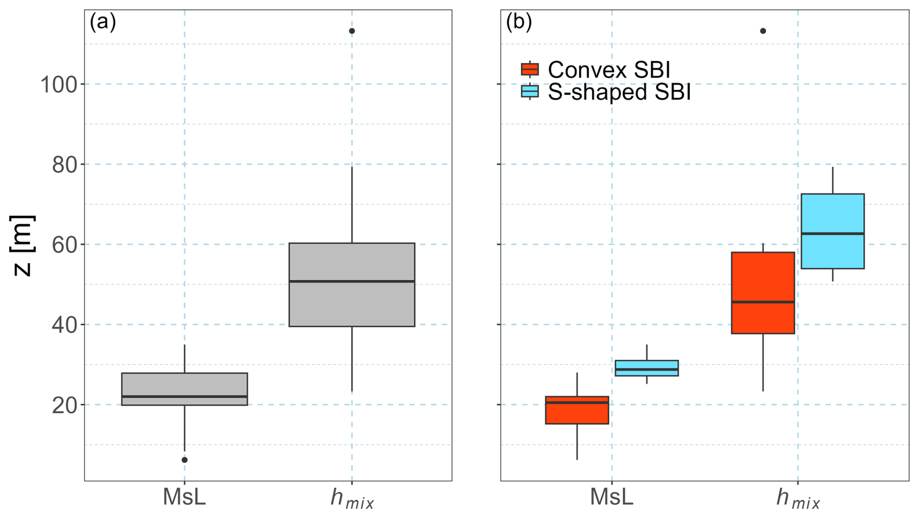
Figure 7 (a) Box plots of the mixed sublayer (MsL) height and mixing layer height (h_mix) for cases of the stable boundary layer. (b) Same as panel (a) but cases of convex and S-shaped SBI are shown separately. The thick horizontal line represents the median, the box the interquartile range and the whiskers' lengths are equal to 1.5 times the interquartile range.

4.2 Comparison of h_mix to the temperature profile

In general, we observe a good correlation between the concentration profiles and the temperature profiles. To evaluate whether the temperature profile alone can be a good predictor of the mixing layer height, we compared it to the observed h_mix. One method to evaluate the height of the SBL is to identify the top of the SBI (i.e., height where the temperature gradient becomes negative) (Seidel et al., 2010). However, the detailed inspection from our in situ measurements revealed that the stratified layer of the SBI (i.e., layer of strongest temperature gradient) seemed to be a more appropriate indicator of h_mix. Because of the stratified nature of the SBIs in central Alaska, the height where the temperature profile returns to a negative gradient (i.e., true SBI top) can be substantially higher than the height of the strongest temperature gradient. Furthermore, as indicated in Bourne et al. (2010), stronger SBIs typically have a higher depth. However, stronger temperature inversions are likely associated with a higher stability and a lower h_mix. Using the SBI top as a predictor of h_mix is therefore not relevant and can lead to large overestimations of the latter. Therefore, instead of using the top of the SBI as a predictor of h_mix, we used the top of the stratified layer. In cases of a convex SBI, the top of the stratified layer is defined as the top of the first layer near the ground (layer with the strongest temperature gradient), identified by the Fochesatto (2015) temperature layer detection algorithm. In cases of an S-shaped SBI, the top is defined at the top of the second layer (capping layer).

Figure 8 shows the relation between h_mix and the top of the stratified layer. The color of the dots indicates the type of SBI. Generally, h_mix agrees well with the top of the stratified layer, with the exception of a few outliers such as the two red points in the lower right corner of Fig. 8. An analysis of these profiles shows an EI located near h_mix, suggesting that the SBI only recently developed and no shallower mixing layer had developed yet. Excluding these outliers, a linear regression through the data points shows a slope of 1.10 with an R² of 0.94, indicating that h_mix is usually located slightly lower than the top of the temperature stratification.

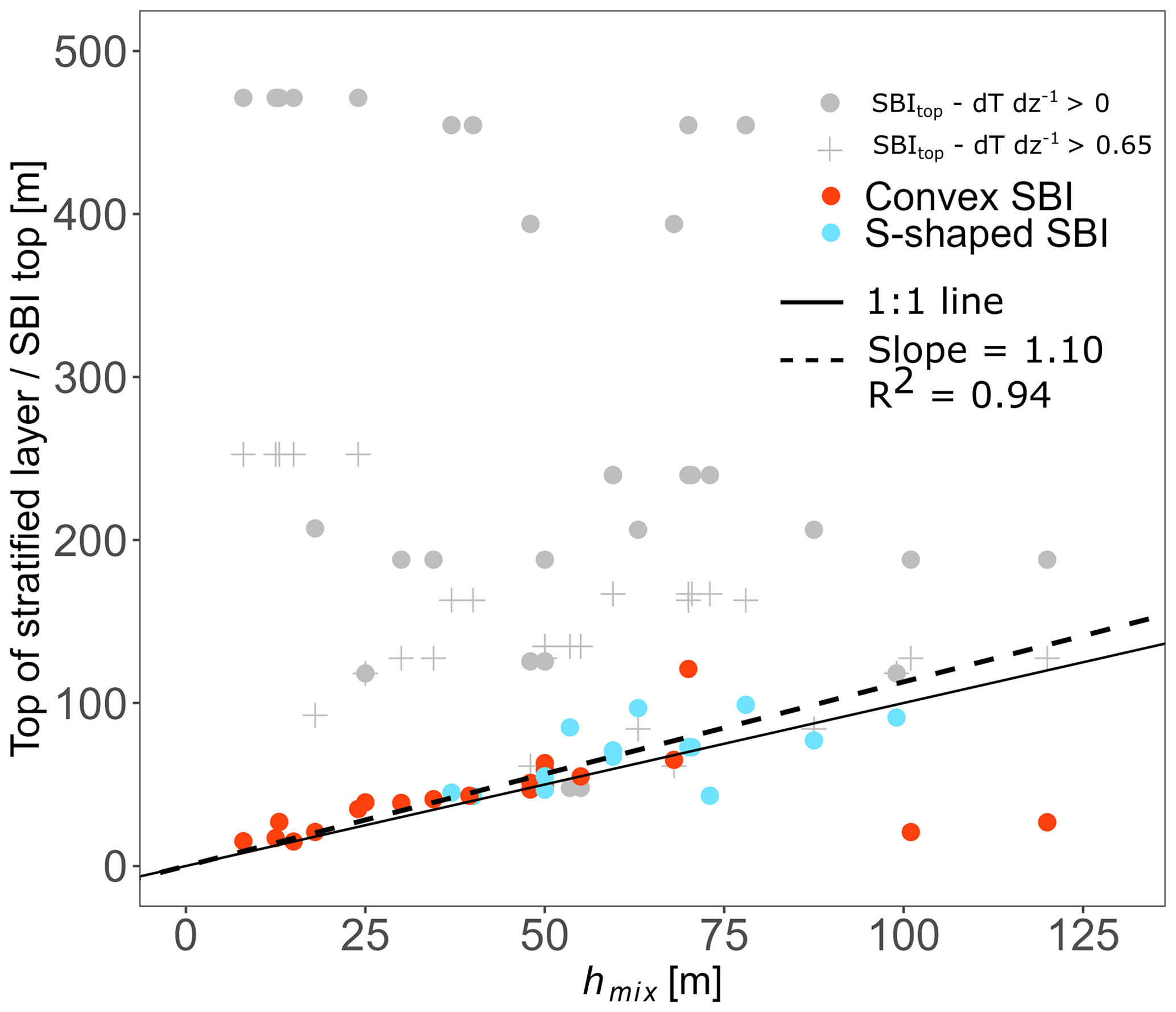
Figure 8 Comparison between h_mix and the top of the stratified layers and SBI top. The top of the stratified layer for convex cases is the top of the first layer (strongest temperature gradient) and top of the second layer for S-shaped cases, indicated by the color of the dots. Grey dots (crosses) indicate SBI top retrieval with a $\mathrm{d}T/\mathrm{d}z$ threshold of 0 °C per 100 m (0.65 °C per 100 m). The solid line represents the 1:1 diagonal, and the dashed line represents the slope of a linear regression fit through the data points corresponding to stratified layer heights.

To illustrate the difference between the top of the stratified layer and the top of the SBI, Fig. 8 also shows the SBI top for each profile, retrieved from the closest radiosounding in time (because Helikite flights did not always allow retrieval of the SBI top due to their limited maximum altitude). Radiosondes are released from the Fairbanks International Airport (PAFA), located 4 km south of the UAF farm site, every 12 h.

The SBI top was retrieved using the algorithm from Kahl (1990). Inversion layers were identified when the temperature gradient was positive (> 0 °C per 100 m) and at least 25 m thick. Inversion layers separated by less than 50 m were merged together. The top of the inversion layer starting from the ground is the SBI top. Since the high-latitude lower atmosphere can sometimes conserve a slightly positive temperature gradient above an SBI, Jozef et al. (2022) have adapted the temperature gradient threshold to 0.65 °C per 100 m for Arctic conditions. We also ran the SBI detection algorithm for this threshold to see whether it would improve the correspondence between the SBI top and h_mix. Figure S5 shows an example of a radiosounding profile with the different SBI tops and the observed h_mix. Grey dots (crosses) in Fig. 8 indicate the comparison of h_mix with the SBI top with the 0 °C per 100 m (0.65 °C per 100 m) threshold.

Overall, the top of the stratified layer is typically very similar to h_mix. It constitutes therefore a much better approximation for h_mix than the SBI top. Conversely, the SBI top is typically located on average roughly 9 (7.5) times higher than h_mix with the 0 °C per 100 m (0.65 °C per 100 m) threshold. These results are in agreement with previous studies that show that the SBI depth over Fairbanks in January and February is typically of a few hundred meters (Bourne et al., 2010), which is much higher than the observed h_mix, which is limited by the lack of turbulence. Processes shaping the temperature profile of the high-latitude wintertime lower troposphere can happen on timescales that vary from hours to several days (e.g., radiative cooling, adiabatic warming from air subsidence, air mass advection) (Fochesatto, 2015). At lower elevations (first tens of meters above ground), the temperature profile might react faster to changes in the surface energy budget due to the higher proximity to the ground. Consequently, changes in the vertical extent of the ML might occur on a much shorter timescale than those defining the entire structure of the SBI, explaining the differences between h_mix and the SBI top.

As the total volume of pollution mixing depends on h_mix and the height of the MsL, an overestimation of h_mix could lead to a pollution concentration underestimation. Therefore, our results show that the stratified temperature layers are a key component of the vertical mixing of pollution, and an accurate representation of the vertical temperature stratification is essential to predict pollution at different heights. In contrast, using the SBI top as an indicator of predicting the vertical extent of pollution mixing would lead to a large overestimation of h_mix. In addition, capturing the strength and persistence of SBIs is essential to realistically estimate air pollution levels over time.

Representing strong SBIs in models remains a challenge, and important positive temperature biases and misrepresentations of the SBI strength and height are commonly observed when models are compared to observations (Mölders and Kramm, 2010). Furthermore, in some locations, such as the UAF farm site, topography plays an important role in the development of local winds that influence the development of inversions and hence has to be represented accurately. This can become challenging when the spatial resolution of models is too coarse.

While the results presented in this section provide a direct assessment of the mixing layer height in the stable boundary layer around Fairbanks, tethered-balloon measurements do not represent a practical method for routine operations. To understand whether h_mix can be predicted from ground-based measurements alone, a comparison between the observed h_mix and formulations of the SBL height based on surface flux measurements was performed. Details on the formulations and all results are presented in the Supplement. Generally, all models have a negative bias and large root mean squared error in comparison to our derived h_mix, indicating that the extremely stable conditions observed in Fairbanks might represent a limit to these models, which further motivates the need to investigate pollution dispersion in the very stable boundary layer.

5 Vertically resolved microphysical properties and chemical composition of the lower atmosphere

To investigate the vertical distribution of aerosols and trace gases, vertical scaling (normalization of the altitude) based on the observed h_mix was applied to all profiles. The results for all profiles are shown in Fig. 9. The top panels represent aerosol characteristics, and bottom panels represent trace gas mixing ratios. All profiles except for σ_geom and the count median diameter (CMD) (panel b) are expressed as the difference compared to the WPBL average concentration (an example of a pollution distribution across a vertical profile is given in Fig. S7). The vertical axis $z/h_{\mathrm{mix}}$, with z representing the height above ground level, has a value of 1 at the top of the ML (horizontal dashed line). This general analysis shows how the pollution profile in the SBL evolves with altitude and reaches values of the WPBL above $z/h_{\mathrm{mix}}$ = 1. We also observe an important variability in concentrations in the MsL, reflecting the various factors influencing pollution in the SBL, including pollution mixing and various emission sources. Figure S8 shows each individual profile expressed in absolute measured values and color-coded by the SBI type. For σ_geom and CMD, we observe an increase in both quantities above h_mix. The observed shift is explained by a PNSD dominated by freshly emitted Aitken mode particles in the ML. Above the ML, the air is more diluted with background air that contains larger aerosol particles. This results in a shift toward a larger σ_geom and CMD. A detailed analysis of the PNSD in each layer is discussed in Sect. 5.3.

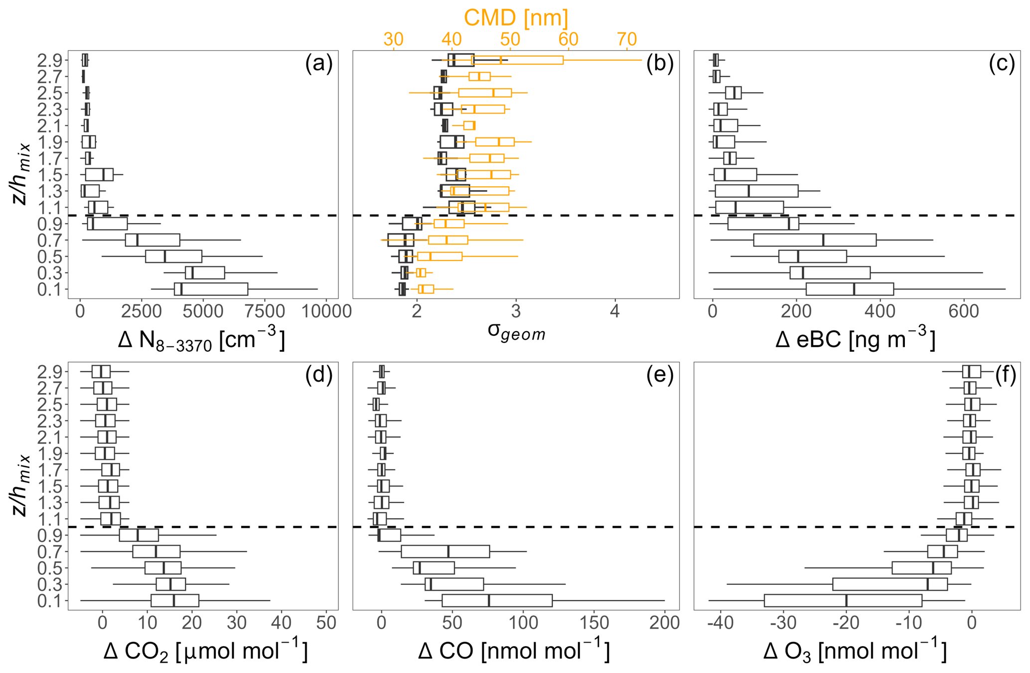
Figure 9 Vertically normalized analysis of various tracers' profiles: (a) N₈₋₃₃₇₀, (b) σ_geom and CMD (orange) of the PNSD from 8 to 270 nm, (c) equivalent black carbon concentration, (d) CO₂ mixing ratio, (e) CO mixing ratio, and (f) O₃ mixing ratio. All values except for panel (b) are expressed as the difference in the profile's WPBL average concentration. The altitude z is normalized by h_mix. The box plots represent the median and interquartile range; the whiskers' length equals 1.5 times the interquartile range.

To quantitatively assess pollution enhancement in the SBL, Fig. 10 compares values of absolute concentrations in the MsL and in the WPBL to the lowest observed background and to the flights with no SBI. The lowest observed background was evaluated from flights where the balloon reached above an EI (eight profiles from four different flights). In the LBL, the concentrations of various tracers dropped even below those in the WPBL. Figure S9 illustrates such a profile. For CO and O₃, no measurements were obtained during these flights. For flights where the boundary layer did not feature an SBI, the measured concentration profiles were typically homogeneous throughout the column. These flights are classified hereafter as no-SBI flights. For no-SBI flights, the concentrations below 22 m (median height of the MsL for cases with an SBI) were used for comparison with the MsL concentrations in SBL cases. The results are shown for two size ranges (8 to 186 nm and 186 to 3370 nm) and for eBC (Fig. S10 shows the results for CO₂, CO and O₃).

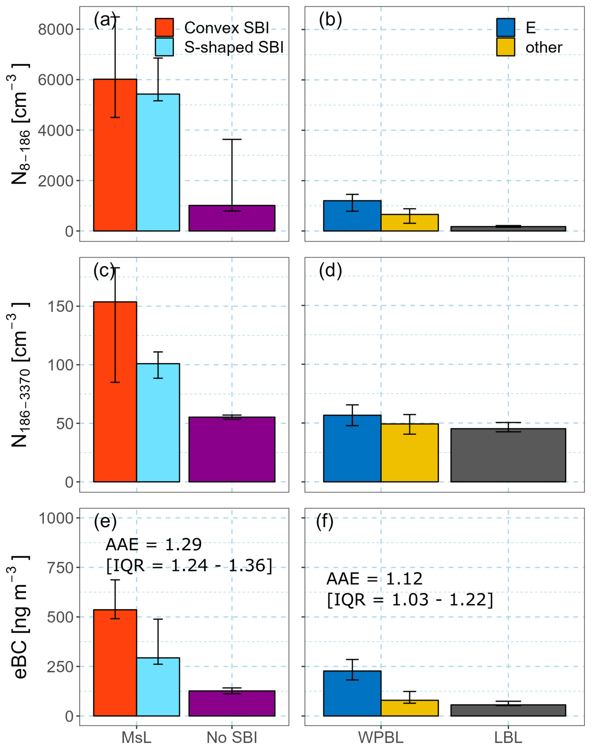
Figure 10 Median aerosol number concentrations from 8 to 186 nm (a, b) and from 186 to 3370 nm (c, d) and eBC mass concentration (e, f). Panels (a, c, e) show values in the mixed sublayer (MsL) under conditions of convex SBI (red) and S-shaped SBI (blue) and without an SBI (purple). Panels (b, d, f) show values in the WPBL under different dominant wind directions (blue and yellow) and in the LBL (grey). The error bars indicate the interquartile range. The absorption Ångström exponents are indicated for the MsL and the WPBL.

5.1 Concentration levels in the MsL

For the MsL, the concentration levels are evaluated separately for cases of convex and S-shaped SBIs (Fig. 10, left panels) to determine the effect of the SCF on pollution levels. To evaluate the general effect of SBI on pollution at breathing level, concentrations for no-SBI flights are shown in the left panels as well (purple bars). Figure 10a, c and e indicate that under S-shaped SBI conditions, the concentration levels are generally lower than under convex SBI conditions. In comparison to no-SBI situations, the median of N₈₋₁₈₆ is up to 6 (5.5.) times higher under convex (S-shaped) SBI situations. For N_186−3370, the concentration is 3 times higher for the convex SBI and 2 times higher for the S-shaped SBI. Similar differences are observed for eBC. The same observations are valid for gases (Fig. S10) where both CO₂ and CO are higher, and O₃ is lower due to increased titration from NO emissions under convex SBI cases. Compared to no-SBI situations, CO₂ increases by 17 and 10 ppm for convex and S-shaped SBIs, respectively. O₃ is more depleted for convex SBIs with a median of 16 and 30 nmol mol⁻¹ for S-shaped SBIs (33 nmol mol⁻¹ for no-SBI situations). Interestingly, the difference in O₃ between S-shaped SBI and no-SBI situation is very small. A possible explanation could be that with a stronger SCF, air with higher O₃ mixing ratio from upper levels is brought down from the surrounding hills, eventually leading to increased O₃ mixing ratios compared to situations with a weaker SCF.

There are no available measurements for CO under no-SBI situations, but MsL median values equal 237 and 185 nmol mol⁻¹ for convex and S-shaped SBIs, respectively. All values presented in Figs. 10 and S10 are summarized in Table S5 for the different layers and situations.

Overall, the observed higher concentrations under convex SBI situations are consistent with the MsL and ML height differences observed in Sect. 4.1 and suggest that the mixing and ventilation from the stronger SCF (S-shaped SBI) increase pollution dilution. Also, the source region of the SCF has fewer emission sources than the Fairbanks area and therefore would typically not transport larger pollution levels. For the convex SBI, the SCF is weaker (or inexistent), and when easterly synoptic winds dominate, advection from Fairbanks contributes to the surface pollution observed, leading to higher pollution levels compared to cases of S-shaped SBI (Fochesatto et al., 2024). The effect of the SCF is rather localized, as it is confined to the Goldstream Valley and the area around the UAF farm site. Here, the valley opens into a wider plain, which reduces the wind speed of the SCF. Because of the reduced speed and the urban canopy, the SCF was only rarely observed at the CTC site during the campaign. Figure S11 shows simultaneous wind measurements at both sites. The results indicate that when a 1.5 m s⁻¹ threshold is applied (limit for a significant SCF detection), a SCF was detected 52.3 % of the time at the UAF farm compared to 0.6 % at CTC. The results presented here are therefore specific to the UAF farm site. It has also been shown by Robinson et al. (2023) that, under strong SBI situations, the pollution distribution across the city was highly heterogeneous from one neighborhood to another as a result of poor vertical and horizontal dispersion, confirming that our observations are likely not representative of all of the Fairbanks area. In the center of Fairbanks, we generally suspect situations of strong radiative cooling, i.e., periods when the SCF develops at the UAF farm, to be associated with even stronger capping of surface emissions with a convex SBI, because typically the SCF does not influence the downtown area as much.

5.2 Concentration levels above the ML

Above the ML, concentrations are lower, as shown in Fig. 9. Figure 10b, d and f show the measured absolute concentrations in the WPBL and in the LBL. Concentrations in the WPBL are evaluated separately based on the dominant wind direction sector to evaluate the outflow from Fairbanks (easterly wind) above the ML. Dominant wind directions were determined by the wind lidar at the height levels corresponding to the WPBL. A dominant easterly wind direction was observed (defined for winds between 45 and 135°). Other dominant wind directions in the WPBL were either from the north (winds between 315 and 45°) or from the south (winds between 135 and 225°). A Mann–Whitney test on the concentration distributions from the north and the south indicated that there was no significant difference between the observed median concentrations (p value ≪ 0.01). North and south advection situations were therefore merged together and categorized as “other”. The grey bars in the right panels represent the concentrations measured in the LBL for each tracer. Generally, easterly advection leads to more elevated concentration levels compared to other wind directions, indicating a direct influence from Fairbanks and likely from nearby power plants, which are all located to the east. For northerly and southerly advection situations (yellow bars), concentration levels are very similar to the LBL levels (indicated by the grey bars) except for N₈₋₁₈₆ (Fig. 10b), where the median concentration is almost 4 times the LBL level, indicating that some of the smaller particles trapped in the WPBL could remain there for a longer time and be recirculated around Fairbanks as the wind direction changes. In cases of easterly advection, the median of the particle number concentration (N₈₋₁₈₆) is > 1200 cm⁻³, 7 times the value measured in the LBL (174 cm⁻³). For other wind directions, the median concentration is 670 cm⁻³, 4 times the LBL concentration. The number concentration of particles larger than 186 nm (Fig. 10d) is only marginally higher than this background, which supports the hypothesis that the WPBL is mainly enhanced in small particles that are less aged than background aerosols. For eBC, concentrations are significantly elevated during easterly advection compared to other wind directions, with levels (230 ng m⁻³) nearly matching those observed in the MsL during S-shaped SBI conditions (290 ng m⁻³). In the LBL and in the WPBL with other advection situations, the median observed concentrations equal 56 and 80 ng m⁻³, respectively. These observations suggest a significant influence of local soot emissions on the pollution in the WPBL. To evaluate differences in eBC sources in the MsL and in the WPBL, the Ångström exponent (AAE) was compared between the layers. The AAE has a median value of 1.29 [IQR = 1.24–1.36] and 1.12 [IQR = 1.03–1.22] in the MsL and in the WPBL, respectively. A Mann–Whitney test indicated that the difference between the median values was different from zero (p value ≪ 0.01). Generally, lower values of AAE (closer to 1) can be attributed to black carbon (BC) from fossil fuel emissions, while higher values indicate the presence of other absorbing species, including brown carbon (BrC) from biomass burning (Andreae and Gelencsér, 2006; Bond et al., 2013; Bond and Bergstrom, 2006; Helin et al., 2021; Moschos et al., 2021). The higher AAE values in the MsL suggest a higher variability in sources contributing to the overall load of eBC, including biomass burning from domestic wood burning or other combustion sources, which remain trapped in the ML. Robinson et al. (2023) measured AAE values above 1.4 in residential areas in the eastern part of Fairbanks when strong SBIs were identified at the UAF farm site, confirming the contribution from biomass burning to the eBC concentration. In the WPBL, fossil fuel sources seem to be the largest contributor to eBC concentrations because of the lower AAE value. Potential sources include the power plants with high stacks directly emitting above the SBL and ones that are mainly powered by coal or diesel (see Table S7; Brett et al., 2025). The contribution from power plants is discussed in Sect. 6.

We compare here values of the WPBL and LBL to previous measurements of Arctic or sub-Arctic background values to put these observations into a wider perspective and understand the impact of a city like Fairbanks on pollution export to the Arctic. We consider hereafter both in situ measurements in the free troposphere from mobile platforms (aircraft or tethered balloons) and from remote high-latitude locations during winter or early spring representative of surface-based Arctic haze values. Details on the different studies used as a reference, the location and period of measurements are provided in the Supplement, and all values are provided in Table S5. Generally, the measured LBL aerosol concentrations fall within similar ranges to the background references, while the WPBL exhibits significant enhancements for the integrated particle number concentration and eBC as described above.

In April 2008, during the Aerosol, Radiation, and Cloud Processes affecting Arctic Climate (ARCPAC) project, an aircraft measured the free-tropospheric background haze concentrations above northern Alaska (Brock et al., 2011). The concentration of submicron aerosol particles had an average concentration of 371 cm⁻³. Additionally, Freud et al. (2017) reported concentrations between roughly 190 and 250 cm⁻³ in the size range 10 to 500 nm at Utqiaġvik/Barrow for the months of January and February. These values are similar to our observations in the LBL (219 cm⁻³ for a size range 8 to 3370 nm). Although the reported size ranges vary slightly between each study, they cover the Aitken and accumulation modes, which are the main contributors to the number concentration (discussed in Sect. 5.3). Note that the higher concentrations reported by Brock et al. (2011) could be explained by the natural heterogeneity of the aerosol spatial and temporal distributions, as the reported values were limited in time. Their measurements could have also captured high-pollution-transport events from lower latitudes, at higher altitudes in the free troposphere. Finally, from annual cycles of the evolution of Arctic haze (e.g., Boyer et al., 2023; Freud et al., 2017), we can assume that slightly higher number concentrations are expected in April, the peak of the Arctic haze season.

For eBC, the concentration in the LBL (56 ng m⁻³) is very similar to what was reported by Brock et al. (2011) for the FT haze background (60 ng m⁻³) and at Utqiaġvik/Barrow for the months of January and February (58 ng m⁻³, median value for the period 1992–2019) (Boyer et al., 2023; Schmale et al., 2022). Here again, the outflow from Fairbanks in the WPBL may constitute a significant contribution to the Arctic-wide transport of black carbon below elevated inversions (230 ng m⁻³). Upper-level transport of eBC was also observed in profiling studies performed over Ny-Ålesund (e.g., Cappelletti et al., 2022; Ferrero et al., 2016; Markowicz et al., 2017; Mazzola et al., 2016). Increasing concentrations with altitudes up to 1000 m above ground level (a.g.l.) with values between 100 and 300 ng m⁻³ were reported by Mazzola et al. (2016). Cappelletti et al. (2022) reported mean concentrations of 110 ± 10 and 150 ± 30 ng m⁻³ below and above 500 m, respectively. Ferrero et al. (2016) identified different atmospheric profile types during spring. Their “decoupled negative gradient” (DNG) type presents a similar thermodynamic structure to the profiles observed in Fairbanks with an SBI and an EI. For these types, eBC was more elevated between the SBI and the EI, with mean concentrations of 121 ± 5 ng m⁻³. This situation is similar to what we observe in the outflow of Fairbanks above the ML, which illustrates similarities to the efficient and direct transport of anthropogenic emissions (Stohl et al., 2007). Differences between our study and measurements in Ny-Ålesund come from the distance to the emission sources. In our study, the highest concentration of eBC is still observed at the surface due to the presence of emission sources.

The enhancement in N₈₋₁₈₆ and eBC in the WPBL compared to the LBL suggests here that the outflow from Fairbanks trapped below the EIs could be a large source of aerosol particles in the lower atmosphere and contribution to the Arctic haze. Similar processes likely occur in other high-latitude cities.

Regarding trace gases, no CO or O₃ measurements were obtained in the LBL. CO values in the WPBL (121–148 nmol mol⁻¹) are overall slightly lower than those reported by Brock et al. (2011) (161 ± 8 nmol mol⁻¹) but very similar to those reported by Kinase et al. (2025) (131 [107–150] nmol mol⁻¹) at the Poker Flat Research Range, 30 km north of Fairbanks, and by Whaley et al. (2023) at Utqiaġvik/Barrow (∼ 140–150 nmol mol⁻¹) (surface measurements). These relatively low values compared to the MsL at the UAF farm site (237 [200–255] nmol mol⁻¹) indicate that CO emissions above the ML are relatively low and reveal potentially good combustion efficiencies of elevated emission sources, as discussed in Brett et al. (2025). Different emission sources and their link to CO emissions in the WPBL are discussed further in Sect. 6.2. Median O₃ in the WPBL equals 38 nmol mol⁻¹ for easterly (Fairbanks direction) and other wind directions. The similarity in O₃ values indicates that NO emissions in the WPBL outflow from Fairbanks are probably not high enough to detect a significant decrease in the O₃ mixing ratio. Brock et al. (2011) reported values of 52 nmol mol⁻¹ in the free troposphere. This higher value is likely related to the higher incoming solar radiation in April compared to January and February. Whaley et al. (2023) reported values between 32 and 40 nmol mol⁻¹ for Arctic stations during January and February, very similar to our observations.

Overall, values of particle number concentration in the LBL are either similar to or slightly lower than the reported high Arctic haze background values used for comparison. In the WPBL, especially under easterly winds from Fairbanks, aerosol particles and eBC concentrations are significantly enhanced compared to reported background values in the free troposphere or at Arctic stations, while trace gases are more similar.

5.3 Analysis of the particle size distributions in different layers

To more effectively evaluate the various contributions and enhancements to the aerosol population across different layers, we also analyzed the aerosol particle size distributions (number and volume) for each layer. Figure 11a shows the results for the particle number size distribution in the MsL, the WPBL and the LBL, and from the ground-based station during Helikite flights. Panel (b) shows the PNSD normalized to vector length (i.e., divided by integrated concentration) to better compare the relative contribution and location of each mode of the size distributions. Figure 11c and d show the same but for the particle volume size distribution (PVSD). The size range in Fig. 11 is from 10 to 500 nm because concentrations above 500 nm are very small (several orders of magnitude lower) compared to the maximum observed concentrations. The extended size distributions up to 3370 nm are shown in Fig. S12. Table S6 shows the results of lognormal fit parameters of the PNSD in each layer. To simplify the figure, the size distribution in the MsL is shown for both types of SBIs together, since a comparison showed very similar size distributions.

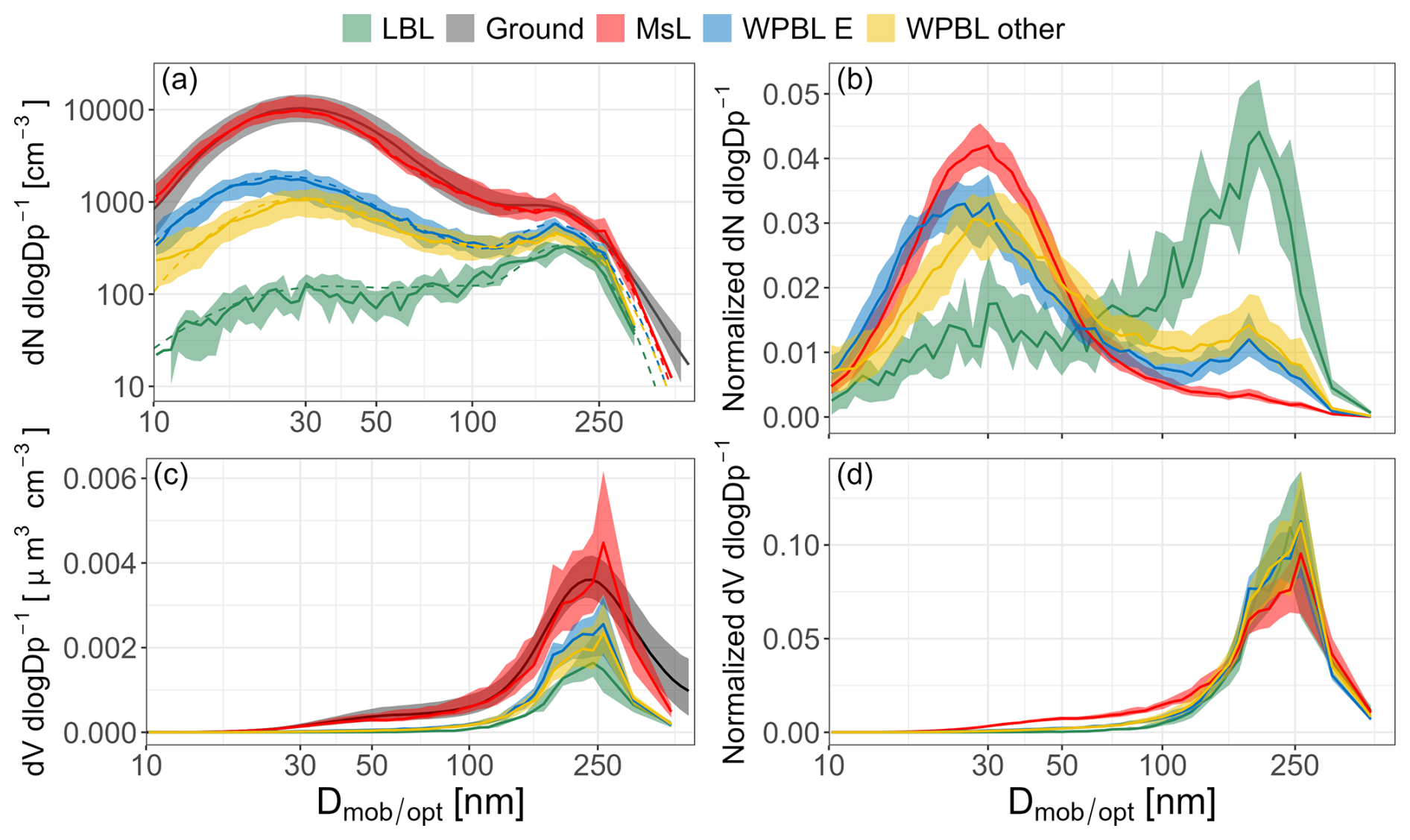
Figure 11 (a) Particle number size distribution in the mixed sublayer (red), in the weakly polluted background layer under easterly dominant winds (blue) and other wind directions (yellow) and in the free-troposphere background layer (green). (b) Normalized PNSD in the same layers. (c) PVSD in the same layers. (d) Normalized PVSD in the same layers. The displayed size range is from 10 to 500 nm and is merged from the mSEMS and the POPS. Solid lines and shaded areas represent the median and interquartile range of the PNSD, respectively. The dashed line in panel (a) represents the fitted PNSD. Fit parameters are indicated in Table S6.

We find bimodal PNSD (Aitken and accumulation mode) with differences in magnitude and relative contribution of each mode in the different layers. The accumulation mode is dominant in the LBL, as indicated by the green distribution (mode peak at 193.1 nm). The observed distribution is very similar to the distribution observed by Freud et al. (2017) at Utqiaġvik/Barrow for the months of January and February and to their accumulation mode cluster (cluster 1) representative of Arctic haze. The PNSD observed at the Zeppelin station before the summer transition (April) by Engvall et al. (2008) also shows a very similar structure. Together with the total number concentration comparison (Sect. 5.2), these results indicate that the measurements in the LBL are likely to be representative of the free-tropospheric haze background for the winter months.

In the MsL and the WPBL, an Aitken mode from the fresh pollution dominates the number concentration. The Aitken mode in the MsL has a peak at 28.8 nm with a standard deviation of 22.1 nm. The PNSD measurements performed on the ground (grey distributions) during the vertical measurements show very good agreement with the measurements of the MsL.

In the WPBL under easterly advection from Fairbanks, we observe an Aitken mode peak at 26.0 nm, which is not statistically different from the MsL mode diameter given the uncertainty of the size detection by the instrument (Pohorsky et al., 2024). However, when the wind arrives from other directions in the WPBL, the mode diameter is significantly larger with 32.6 nm. This shift is indicative of the growth of the Aitken mode particles and is consistent with the hypothesis of pollution recirculation in the WPBL, since recirculated particles are older and therefore likely larger due to aging.

In the WPBL, the relative contribution of the accumulation mode to the PNSD is larger than in the MsL (Fig. 11b). This larger relative contribution is mainly due to lower concentrations in the Aitken mode since there are similar absolute concentrations in the accumulation mode in all layers, including the FT background. The larger relative contribution in the accumulation mode is reflected in the calculation of the σ_geom and CMD, which explains the consistent shift to larger values observed above the SBL (Fig. 9b).

The particle volume size distributions and, in comparison, the mass size distributions are dominated by accumulation mode particles, with a peak of around 250 nm in all layers. An analysis of the extended volume size distribution up to ∼ 3 µm (see Fig. S12) revealed that contributions to the mass from larger particles were much lower (< 1 %) at the surface, indicating that the particulate mass is essentially driven by submicron particles and well represented by Fig. 11. The volume (and therefore also mass) concentration difference in the various layers is primarily driven by differences in the accumulation mode concentration. However, the PVSD in the MsL exhibits a larger tail towards smaller particle diameters, suggesting a more significant contribution to the mass from Aitken mode particles as well.

6 Analysis of elevated sources of pollution

As discussed in Sect. 5.2, with easterly winds the WPBL shows increased pollution compared to the LBL. These measurements provide insights into the amount of pollution exported from a high-latitude city like Fairbanks, contributing to the Arctic haze, as discussed in the section above. Generally, upward mixing between the ML and WPBL, especially during SBI breakups, can represent a source of pollution in the WPBL, but direct emissions at higher altitudes are another source. Here, we show that emissions from power plants are likely an important contributor to the elevated pollution concentrations aloft due to the height of their stacks and the buoyancy of the emitted plume. On several occasions, plumes from different power plants were advected above the UAF farm site and observed in situ during Helikite flights, which allowed us to measure their composition. While most studies so far in the Fairbanks area have provided information on pollution measurements at the surface (e.g., Moon et al., 2024; Robinson et al., 2024; Tran and Mölders, 2011; Ward et al., 2012), these measurements contribute to identifying the specific pollution signature of power plant emissions. We contrast them against the pollution properties in the MsL.

Hereafter, we present a case study (Sect. 6.1) to describe the characteristics of a power plant plume and then discuss the composition of the observed plumes in comparison to pollution measured at the surface in the center of Fairbanks (Sect. 6.2). This analysis complements and makes use of Lagrangian particle dispersion model simulations of surface and power-plant-emitted tracers during the campaign, which also showed an important contribution from power plant emissions aloft over Fairbanks (Brett et al., 2025). Helikite profiles were used to validate and improve the model results in that study.

6.1 Case study of an observed power plant plume

On 20 February 2022, between 06:00 and 11:00 local time (LT), eight vertical profiles reaching up to 300 m a.g.l. were obtained. An elevated plume was seen in six of the profiles. Figure 12 shows the structure measured in profiles 2 and 4 (descending profiles). Note that profile 2 did not extend all the way to the ground since the Helikite's traveling direction was reversed at 25 m. The lower atmosphere was characterized by a stable boundary layer with an S-shaped SBI up to 60 m and an EI between 184 and 225 m (Fig. 12a).

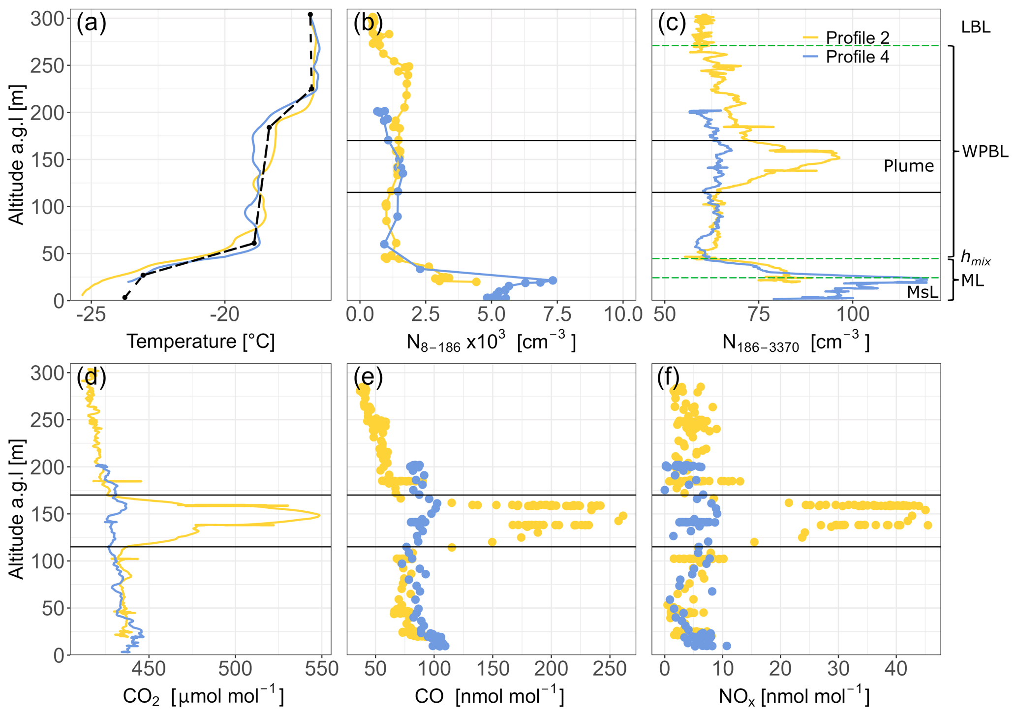
Figure 12 Vertical profiles of (a) temperature (°C), (b) aerosol number concentration from 8 to 186 nm (cm⁻3), (c) aerosol number concentration from 186 to 3370 nm (cm⁻3), (d) CO₂ mixing ratio, (e) CO mixing ratio and (f) NO_x mixing ratio. The yellow color represents the second profile, and the blue represents the fourth profile of a flight performed on 20 February 2022 between 06:00 and 11:00 LT. The dashed black line in panel (a) represents the flight-averaged simplified temperature profile. The horizontal black lines represent the upper and lower edges of the plume. In panel (c), the different layers are indicated in the margin and delimited by dashed green lines.

In profile 2, an elevated plume was captured between 115 and 170 m with a concentration peak at 150 m a.g.l. The plume edges (lower and upper limits) are marked by a strong inflection point in the concentration profiles with an enhancement of N_186−3370 and of all measured trace gases. However, we do not observe an increase in ultrafine particles (N₈₋₁₈₆) in the plume. The plume was still observed in profile 3 (not shown here) but not anymore in profile 4 due to a change in wind direction, from easterly (81°) to more northeasterly (70°).

To identify the source of the observed plume, we used the results from the FLEXPART–Weather Forecasting and Research (WRF) tracer simulations described in Brett et al. (2025). NO_x emission tracers, as enhancements above the background, from the different power plants operating in Fairbanks during the flight period, at the UAF farm site, are shown in Fig. S13. The model results indicate that the plume observed on 20 February originated from the coal-fired generator of the UAF power plant (UAF C; see Table S7) with a stack height of 64 m, located 1740 m to the east of the UAF farm site.

From the concentration profiles, we can calculate the maximum excess in the plume compared to the WPBL and the MsL for each tracer. A tracer's plume excess is obtained by subtracting the background (i.e., no plume) average concentration values measured in the WPBL or in the MsL from the values measured in the plume, as for example, in Hobbs et al. (2003). Therefore,

$$\begin{array}{}\text{(7)}& \mathrm{\Delta }X=X_{\mathrm{plume}}-X_{\mathrm{ref}},\end{array}$$

where ΔX represents the enhancement of a tracer inside a plume, X_plume is the measured concentration in the plume and X_ref is the average reference concentration (i.e., WPBL or MsL). We calculate ΔX relative to both the WPBL and MsL to compare the plume concentrations with each of these layers. Units are in cm⁻³ for aerosol number concentration and nmol mol⁻¹ or µmol mol⁻¹ for trace gases.

The maximum accumulation mode particle enhancement (ΔN_186−3370) observed in the plume with respect to the WPBL value was ∼ 30 cm⁻³; for the trace gases, the enhancements were as follows: ΔCO₂ ∼ 116 µmol mol⁻¹, ΔCO ∼ 190 nmol mol⁻¹ and ΔNO_x ∼ 42 nmol mol⁻¹. With respect to the MsL average values, particle number concentrations show little enhancement, but trace gas concentrations are enhanced in the plume: ΔCO₂ ∼ 108 µmol mol⁻¹, ΔCO∼ 160 nmol mol⁻¹ and ΔNO_x ∼ 38 nmol mol⁻¹.

These enhancements are, however, only indicative, as it is uncertain how the ΔX of a certain tracer evolves from the edge to the center of a plume. Given the observed dynamics described above, it is however likely that the observations were made on the edge of the plume, where the enhancements are expected to be lower compared to the center of the plume.

We can nevertheless compare the observed ratios between pairs of different tracers in the plume to those observed in the SBL. The particulate-to-gas ratio (e.g., $\mathrm{\Delta }{N}_{\mathrm{186}-\mathrm{3370}}/\mathrm{\Delta }$CO) is typically lower in the plume than in the MsL. The absolute values of N_186−3370 in the plume and the MsL are very similar, with a maximum concentration of 96 cm⁻³ in the plume and an average concentration of 100 cm⁻³ in the MsL. The main difference comes from the mixing ratios of trace gases in the plume, which are much higher than those observed in the MsL. Compared to the WPBL, both particles and gases are enhanced in the plume, indicating that power plant plumes can be a significant source of the pollution observed in the WPBL as a result of dilution over time.

To further constrain the plume's origin and assess whether its composition is unique to the UAF power plant, we conducted a systematic analysis of various chemical tracer ratios in plumes and at the CTC site. This analysis also aimed to distinguish these emissions from those of other elevated plumes and surface pollution.

6.2 Analysis of tracer–tracer relationship of plumes

Elevated pollution plumes were measured in 25 profiles from eight different flights during the campaign. Details on the identification of plumes and attributions to different power plants are provided in the Supplement. Here, we analyze the composition of the different plumes. Tracer–tracer relationships are plotted for 10 s averaged data points of ΔN_186−3370 and ΔCO against ΔCO₂ (Fig. 13). CO₂ was used as a reference because it constitutes a passive tracer for anthropogenic emissions and was measured systematically on all flights. N_186−3370 was also systematically measured on all flights and serves as an indicator of particulate matter release from various emission sources. Finally, on the timescale of the plume atmospheric transport to the site, CO can be assumed to be a conserved tracer, and in winter it can also be considered passive, due to very low hydroxyl (OH) levels. Assuming that mixing of the plume emissions with the ambient air is slow compared to the advection timescale, emission ratios can be derived from the tracer–tracer correlation (Andreae and Merlet, 2001).

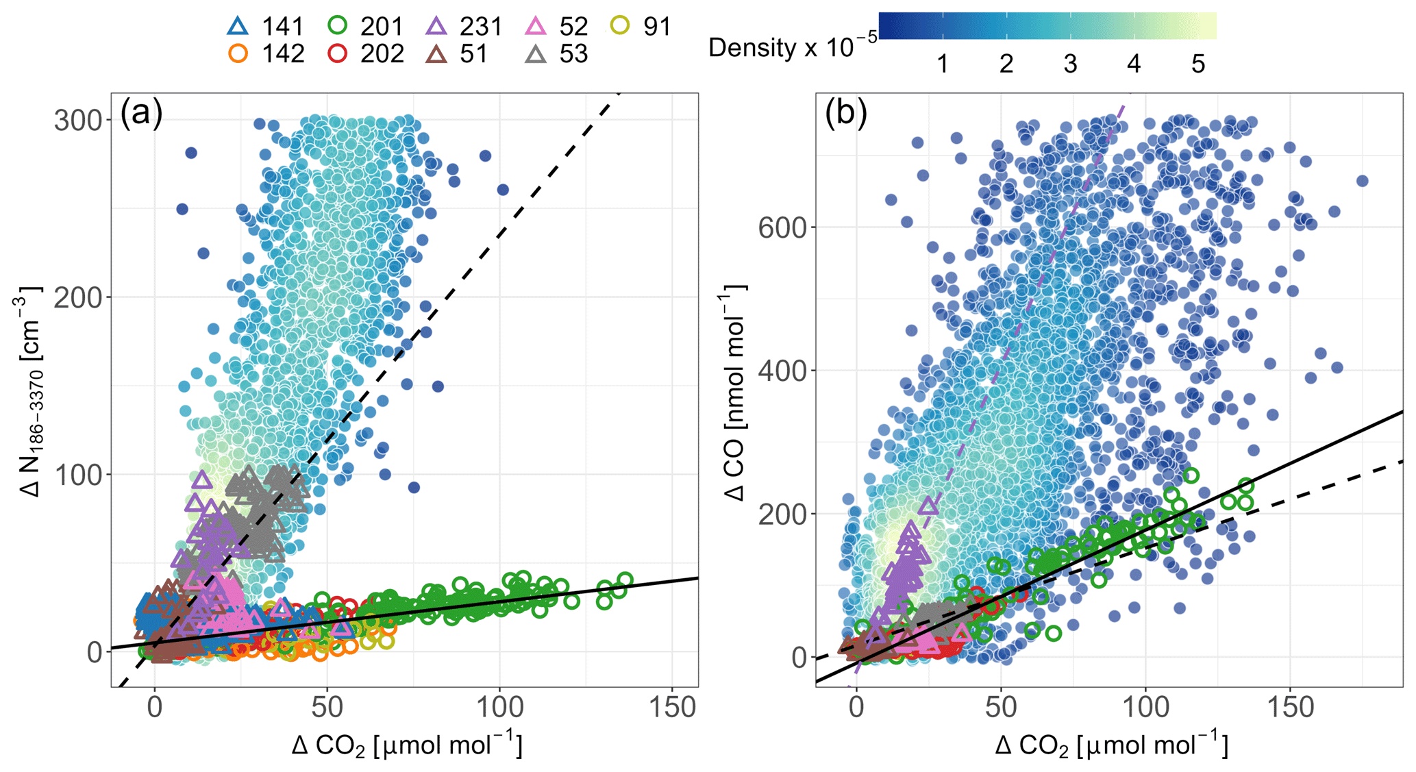
Figure 13 The tracer–tracer relationship of measured elevated plumes compared to ground-based observations in downtown Fairbanks. The different tracers are expressed as concentration enhancements between the measured value in the plume and the average concentration of the WPBL (outside the plume). Circles represent data points from UAF C plumes. Triangles represent data points from other plumes. The solid lines represent a linear regression through data points corresponding to UAF C plumes (coal-fired power plant). The dashed black lines are for the other plumes of uncertain origin (likely coal- and/or diesel-powered power plants). The dashed purple line likely corresponds to a pollution plume originating from Chena Ridge (likely from domestic heating). The dots with the density coloring correspond to tracer–tracer relationships from ground-based measurements at CTC. The color-coding corresponds to the density of the observations.

Markers in Fig. 13 are colored according to the plume ID (see Table S8). Given the uncertainties in the origins of the non-UAF C plumes, the sources of these plumes were classified as “other” and are denoted by triangles. Circles represent plumes from UAF C. Additionally, Fig. 13 shows the ratios measured at the surface at the CTC site (see Fig. 1) during ALPACA. The dots represent 30 min averaged measurements and are color-coded by the number of data points (i.e., density of their overall distribution). The ΔX was calculated using Eq. (7), where X_ref is the 10th percentile of all values. The Δ_particle was calculated from the mobility diameter of a scanning mobility particle sizer (SMPS model 3936, TSI, USA). Number concentrations were integrated from 186 to 650 nm. Although the upper range of the SMPS differs from the POPS (650 versus 3370 nm), the number concentration is strongly dominated by particles smaller than 500 nm (Fig. 11). Differences in total number concentration with an upper range up to 650 or 3370 nm are therefore negligible.

We observe that the plumes exhibit distinct and consistent tracer–tracer slopes, which for UAF C are different from the ratios observed in the other plumes and at the surface. In Fig. 13a, the $\mathrm{\Delta }{N}_{\mathrm{186}-\mathrm{3370}}/\mathrm{\Delta }$CO₂ ratio of the UAF C plume is much lower than for other plumes, specifically plumes 53 and 231. The ratio of the other plumes is more similar to the one observed at the surface. A linear regression through the UAF C plume data gives a slope of 0.24 (±0.01) particles cm⁻³ (µmol mol⁻¹)⁻¹ of CO₂ (R² = 0.66). The slope for the other plumes is 2.32 (±0.09, R² = 0.64).

UAF C is a low-sulfur coal-fired power plant, which is younger than other power plants in Fairbanks and has implemented stricter emission control strategies, which could explain lower particle or particle precursor emissions (ADEC, 2019; Brett et al., 2025). The other power plants are powered by either coal or diesel and are typically older than UAF C. At the surface, the pollution is a mix of various emission sources with main contributions from wood smoke from domestic heating, diesel emissions and automobiles (Ward et al., 2012; ADEC, 2019). These emission sources are likely to emit more primary particles and/or aerosol precursor gases.

Another potential explanation for the different observed $\mathrm{\Delta }{N}_{\mathrm{186}-\mathrm{3370}}/\mathrm{\Delta }$CO₂ ratios could be related to the plume age. Since the Fairbanks power plants are located farther away from the measurement site than UAF C, the plumes were typically older. The average UAF C plumes' age was 20 min, while the other plumes' age was estimated to approximately 1 h on average, based on the average location of the power plants and wind speed at plume height. Given the longer residence time of the other plumes, aging processes (e.g., coagulation and condensation of gases upon existing particles) could have contributed to a larger concentration of particles with a diameter greater than 186 nm (lower cutoff diameter of the POPS). The same logic applies to pollution in the ML, with typical residence times during SBL conditions of a few hours (Cesler-Maloney et al., 2024).

Figure 13b shows the ΔCO $/$ ΔCO₂ ratios that are similar for all plumes, except for plume 231 (purple triangles). The linear regression slope for plume 231 is 0.0085 (±0.0007) mol CO (mol CO₂)⁻¹, 0.0014 (±0.0002) for the other plumes and 0.0019 (±0.00004) for the UAF C plumes. At the surface, we see ratios covering almost the entire range between the power plant plumes and plume 231, but most observations are closer to the ratio of plume 231. The higher ΔCO $/$ ΔCO₂ ratio for plume 231 indicates a less efficient combustion process. An analysis of the potential origin of this plume (see plume identification details in the Supplement) indicates that the plume was likely not from a power plant but from the slope of Chena Ridge (southwest of the UAF farm site). The origin of the plume and the observed tracer–tracer ratios suggest that the plume potentially consisted of wood smoke from domestic heating. These results are supported by the similarity in the observed ratios at the ground, where wood burning represents a major contribution to the pollution in the ML.

The light absorption photometer (STAP) was operated only on one flight when plume 91 was intercepted on 4 February. The STAP data did not show any perceptible increase in light absorption, suggesting that the UAF C power plant did not contribute significantly to the eBC mass concentration observed in the WPBL. However, more measurements should be carried out to provide more robust statistics on light absorption characteristics of power plant plumes and eBC concentrations.

Overall, we observe that power plant plumes have distinct emission ratios compared to what is observed at the surface. These differences can be explained by the fact that observations inside the plumes are typically representative of a single emission source, with limited mixing with background air, given the atmospheric static stability, while observations in the ML are typically the result of the mixing of different sources. Furthermore, the results from Fig. 13b suggest that power plants are usually operated to optimize combustion (i.e., increased conversion to CO₂ and lower CO emissions), while domestic wood stoves or cars are likely to emit relatively more CO. Substantial differences for particulate matter emissions between different power plants are however observed and are potentially linked to differences in fuel types and adopted emission control strategies (ADEC, 2019).

While the Eulerian approach of the Helikite observations (point measurement in the horizontal plane) allows one to measure the different layers of the lower atmosphere and sample plumes from the power plants when the wind direction is favorable, it remains difficult to determine how the plume composition will evolve and whether the plumes contribute to pollution at the surface. Future studies using different methods (e.g., with a Lagrangian approach) are encouraged to address these specific issues. The emission ratios derived from this analysis can nevertheless serve as reference values for future studies aiming at evaluating the impact of emissions from power plants. These results could also be used by environmental protection agencies for comparison with reported emission factors.

7 Conclusions

In situ measurements of the vertical profiles of aerosols and trace gases were carried out at a suburban site near Fairbanks in central Alaska during the winter of 2022 as part of the ALPACA campaign (Simpson et al., 2024; Fochesatto et al., 2024) to explore the vertical distribution of pollution emissions in the highly stratified stable boundary layer (SBL). Over a period of 6 weeks, 148 profiles from 24 different flights were collected up to a maximum altitude of 350 m, constituting an extensive and unique dataset of high-resolution in situ vertical pollution measurements in an urban high-latitude continental boundary layer during winter.

During the campaign, stable boundary layers with surface-based inversions (SBI) were observed in 71 % of the flights. Given the long-lived nature of the SBL during winter in central Alaska, a conceptual schematic of the typically observed vertical structure of the lower atmosphere was introduced (Fig. 5) to better describe our observations. Hence, the mixing layer was divided into a first well-mixed layer called the mixed sublayer (MsL) and a second layer, the mixing layer (ML), containing the MsL and a layer above it with decreasing concentrations. Above the ML, a weakly polluted background layer, here called WPBL, similar but not equal to a residual layer was observed. Pollution in this layer was capped typically under an elevated inversion (EI). Above the EI (in the lowest background layer, LBL), the air contained lower pollution levels than in the WPBL. Concentrations and particle size distribution characteristics in the LBL were similar to previously reported values for free-tropospheric and Arctic haze values.

Our in situ observations allowed the direct assessment of the pollution mixing layer height (h_mix), which had not been directly measured so far, even though it is critical information for air quality modeling. On average, the MsL and the ML have a depth of 22 and 51 m, respectively.

An analysis of the relation between meteorological conditions and the structure of the SBI showed two different modes at the UAF farm site. Under anticyclonic conditions with clear skies, a strong radiative cooling at the surface promoted the formation and strengthening of the SBI, while a local shallow cold flow (SCF) from a nearby valley subsequently became stronger in such situations and increased the shear turbulence near the surface. This situation showed a competing effect between the radiative cooling (strengthening of the static stability) and a local wind (increased mechanical turbulence), leading to an S-shaped SBI with a weaker temperature gradient in the lower few meters near the ground and a capping layer with a stronger gradient above. In conditions with a weaker SCF (lower winds), the SBI had a convex shape with the strongest temperature gradient directly at the surface.

Generally, a good correlation was observed between the height of stratified temperature layers (i.e., layers with the strongest temperature gradient within the SBI) and h_mix. The h_mix was on average at 46 and 75 m for cases of convex and S-shaped SBI, respectively. Hence, under stronger radiative cooling, the effect of local topography on local winds becomes an important factor controlling the vertical mixing of pollution, leading counterintuitively to higher h_mix at the measurement site. The concentration of various tracers was consequently lower for the S-shaped SBI because of a higher mixing layer. These observations complete previous studies at the same site, which already established the role of the local SCF on surface heat fluxes but could not explore these effects on the boundary layer structure or pollution mixing further up.

Our results show that h_mix is typically much lower than the SBI top (Fig. 8), as processes and timescale defining each might be substantially different. Stratified layers with strong temperature gradients in the first tens of meters are much better correlated to h_mix. Hence, while SBIs in Fairbanks typically extend to a few hundreds of meters, a good representation of the temperature profile in the first meters (below roughly 100 m) is essential to predict mixing of surface emissions. While these results might be specific to the measurement site and not fully representative of the larger Fairbanks area due to the local effect of the SCF, situations where the SCF was weak are likely to be indicative of what the depth of the mixing layer can be like in the city center. Our results agree with estimations made from remote sensing measurements at the CTC site (Cesler-Maloney et al., 2024). Given the very shallow ML, even small misrepresentations of the SBI structure can easily have large impacts on the predicted MLH and consequently on the pollution concentration. These results illustrate the need for better representations of the synoptic and local processes shaping the temperature profile of the high-latitude SBL.

A comparison of h_mix with existing parameterizations of the stable boundary layer height (SBLH) based on surface turbulent flux measurements showed that all parameterizations predicted a shallower boundary layer height than the observed h_mix, with large RMSE. These results illustrate the complexity of defining the height of the stable boundary layer and consequently forecasting pollution concentrations.

Above the mixing layer, the pollution concentration drops noticeably but remains slightly higher than in the free troposphere, with clear signs of anthropogenic emissions. A comparison of the observed pollution levels under different wind directions shows that when the main wind direction is from the east, the pollution outflow from Fairbanks significantly increases concentration levels in the upper layers, likely contributing to Arctic haze as it is transported further away. This pollution is typically trapped below elevated temperature inversions. Likely contributors to this pollution are power plants with high stacks. Plumes from different power plants were measured on eight different flights. An analysis of tracer–tracer ratios for aerosol number concentration and CO against CO₂, expressed as delta above a background concentration, revealed distinct mixing lines for different power plants. Differences in Δparticle-to-ΔCO₂ ratios between the UAF C power plant and other power plants and surface emissions were attributed to fuel types and emission control strategies as well as different plume ages. Power plants also seem to be operated in more efficient combustion conditions than other typical pollution sources at the surface (traffic and domestic heating), leading to lower ΔCO-to-ΔCO₂ emission factors in the elevated power plant plumes. Our observations provide a reference for emission factors and encourage future studies to investigate further the aging of power plant plumes in cold and dark conditions and their potential contribution to surface pollution. The study of vertically constrained power plant plumes could also aid in deriving diffusivity coefficients in the various stratified layers for better simulation of vertical pollution mixing.

This study shows that despite existing knowledge about the stable boundary layer in the continental high latitudes, the observed layered structure can be very complex, particularly very close to the surface. Our observations highlight that there is potential to improve the representation of the pollution mixing layer height and elevated plume dilution in, for example, air quality models for better pollution concentration estimates.

Appendix A: Glossary

This is a list of abbreviations. The letter H at the end of an abbreviation refers to the height (top) of a specific layer.

Abbreviation	Definition
AAE	Absorption Ångström exponent
EI	Elevated inversion
FT	Free troposphere
LBL	Lowest background layer
MsL	Mixed sublayer
ML	Mixing layer
MLH	Mixing layer height (= hmix)
SBI	Surface-based inversion
SBL	Stable boundary layer
SBLH	Stable boundary layer height
SCF	Shallow cold flow
VSBL	Very stable boundary layer
WPBL	Weakly polluted background layer