Effects of 2010–2045 climate change on ozone levels in China under a carbon neutrality scenario: key meteorological parameters and processes

We examined the effects of 2010–2045 climate change on ozone (O₃) levels in China under a carbon neutrality scenario using the Global Change and Air Pollution version 2.0 (GCAP 2.0) model. In eastern China (EC), GCAP 2.0 and six other models from the Coupled Model Intercomparison Project Phase 6 (CMIP6) all projected increases in daily maximum 2 m temperature (T2max), surface incoming shortwave radiation (SW), and planet boundary layer height and decreases in relative humidity (RH) and sea level pressure. Future climate change is simulated by GCAP 2.0 to have large effects on O₃ even under a carbon neutrality pathway, with summertime regional and seasonal mean maximum daily 8 h average (MDA8) O₃ concentrations increasing by 2.3 ppbv (3.9 %) over EC, 4.7 ppbv (7.3 %) over the North China Plain, and 3.0 ppbv (5.1 %) over the Yangtze River Delta. Changes in key meteorological parameters were found to explain 58 %–76 % of the climate-driven MDA8 O₃ changes over EC. The most important meteorological parameters in summer are T2max and SW in northern and central EC and RH in southern EC. Analysis showed net chemical production was the most important process that increases O₃, accounting for 34.0 %–62.5 % of the sum of all processes within the boundary layer. We also quantified the uncertainties in climate-induced MDA8 O₃ changes using CMIP6 multi-model projections of climate and a stepwise multiple linear regression model. GCAP 2.0 results are at the lower end of the climate-induced increases in MDA8 O₃ from the multi-models. These results have important implications for policy-making regarding emission controls against the background of climate warming.

1 Introduction

Tropospheric ozone (O₃) is a major secondary gas pollutant produced by the complicated photochemical reactions of methane (CH₄), carbon monoxide (CO), volatile organic compounds (VOCs), and nitrogen oxides (NO_x) in the presence of sunlight. It has adverse effects on human health (Lu et al., 2020; Li et al., 2021; Hong et al., 2019; Dang and Liao, 2019a), ecosystems (Yue et al., 2017; Grulke and Heath, 2020; Ainsworth et al., 2020), and climate (Checa-Garcia et al., 2018; Dang and Liao, 2019a). The Chinese government implemented the Air Pollution Prevention and Control Action Plan in 2013, leading to a large decline in NO_x emissions and PM_2.5 concentrations (Zheng et al., 2018; Zhai et al., 2019), but O₃ pollution in eastern China (EC) became worse over the same time period (Tang et al., 2022; Li et al., 2020; Gong et al., 2020; Dang et al., 2021). Ozone pollution has been particularly severe in the North China Plain (NCP), and observed summer mean maximum daily 8 h average (MDA8) O₃ concentrations increased at a rate of 3.3 ppb yr¹ in NCP from 2013 to 2019, reaching 83 ppb by 2019 (Li et al., 2020). Therefore, it is worth paying attention to the mid- to long-term changes in O₃ concentrations in China in the future.

The projections of future climate or air quality rely on the future emission pathways under different socioeconomic scenario assumptions. Shared Socioeconomic Pathways (SSPs) are state-of-the-art global emission scenarios that combine socioeconomic and technological development with future climate radiative forcing outcomes into a scenario matrix architecture (Gidden et al., 2019). Gidden et al. (2019) constructed nine scenarios of future emissions trajectories, comprising SSP1-1.9, SSP1-2.6, SSP2-4.5, SSP3-7.0, SSP3-LowNTCF, SSP4-3.4, SSP4-6.0, SSP5-3.4-OS (overshoot), and SSP5-8.5. Among all scenarios, only the SSP1-1.9 scenario achieves net negative emissions of carbon dioxide (CO₂) for China and the world by 2060 (Wang et al., 2023), and thus we defined it as a carbon neutrality scenario and applied it in this work. The SSP scenarios are used in Scenario Model Intercomparison Project (ScenarioMIP) in the Coupled Model Intercomparison Project Phase 6 (CMIP6) to facilitate the integrated analysis of future climate impacts, vulnerabilities, adaptation, and mitigation (Gidden et al., 2019; Riahi et al., 2017).

Future O₃ concentrations depend on future emissions. Shi et al. (2021) projected O₃ concentration changes in China over 2020–2060 with no changes in meteorological conditions based on the Chinese Academy of Environmental Planning Carbon and Air Quality Pathways (CAEP-CAP) for pursuing carbon neutrality. The 90th percentile of the daily maximum 8 h average (MDA8) O₃ (90th MDA8 O₃) in China reduced from 138 µg m⁻³ in 2020 to 93 µg m⁻³ in 2060 (a 33 % reduction in 90th MDA8 O₃). Based on the “Ambitious-pollution-Neutral-goal” scenario from the Dynamic Projection model for Emissions in China (DPEC), Xu et al. (2022) used a regional climate–chemistry–ecology model to assess the impacts of regional emission reductions in China with the goal of achieving carbon neutrality by 2060 and found that the national average annual O₃ concentrations would decline by 35.6 µg m⁻³ over 2015–2060. Wang et al. (2023) reported, using the GEOS-Chem model, that the O₃ levels in the Beijing–Tianjin–Hebei (BTH) region, Yangtze River Delta (YRD) region, Pearl River Delta (PRD) region, Sichuan Basin (SCB) region, and Fenwei Plain (FWP) under the SSP1-1.9 scenario could meet the air quality standard by 2030, while those under SSP5-8.5 could not meet it even by 2060. The 90th MDA8 O₃ in BTH, YRD, PRD, SCB, and FWP during 2015–2060 would change by −27.3 %, −27.6 %, −33.1 %, −33.1 %, and −31.8 %, respectively, under the SSP1-1.9 scenario and by +8.6 %, +7.6 %, +5.2 %, −0.5 %, and +2.9 %, respectively, under the SSP5-8.5 scenario (Wang et al., 2023). However, these studies did not examine the effects of future climate change on O₃ concentrations.

Future O₃ concentrations also depend on the future climate. Using the Weather Research and Forecasting Model with Chemistry (WRF-Chem) driven by the Community Climate System Model version 3 (CCSM3), Liu et al. (2013) predicted that climate change caused a 1.6 ppb increase in surface O₃ over southern China in October 2000–2050 under the IPCC A1B scenario. They showed that a future elevated near-surface temperature (1.6 °C) and increased emissions of isoprene (5 %–55 %) and monoterpenes (5 %–40 %) would lead to increases in the chemical production of O₃. Using the GEOS-Chem model driven by the NASA Goddard Institute for Space Studies (GISS) general circulation model (GCM) 3 under the A1B scenario, Wang et al. (2013) reported that climate change would cause a 0.55 ppbv increase in annual mean surface O₃ in EC over 2000–2050, of which more than 40 % could be attributed to climate-induced increases in biogenic VOC (BVOC) emissions. Climate-induced increases in O₃ levels over EC were most pronounced and spatially extensive in summer, with a summer average of 1.7 ppbv and a maximum of 10 ppbv. By employing a combination of models, Hong et al. (2019) projected that warm-season (April–September) averages of daily 1 h maximum O₃ levels would increase by 2–8 ppb in most of EC from 2006–2010 to 2046–2050 under the Representative Concentration Pathway 4.5 (RCP4.5), of which 14 % could be attributable to increased future heat wave days. Based on sensitivity simulations from five CMIP6 models fixing sea surface temperatures (SSTs) in present-day or future conditions in the SSP3-7.0 scenario, Zanis et al. (2022) reported that the sensitivity of O₃ to temperature would be enhanced in regions close to anthropogenic sources or BVOC emission sources (e.g., southern EC), with values ranging from 0.2 to 2 ppbv °C⁻¹. However, the scenarios utilized in these studies were not the representative scenarios in China in the context of carbon neutrality.

Few studies have examined the impacts of climate change under low-carbon or carbon neutrality scenarios. Li et al. (2023) showed, using a machine learning (ML) model along with multi-source data, that the annual mean surface O₃ during 2025–2095 increased by 0–2 ppb over EC under the SSP1-2.6 scenario, with reduced relative humidity and enhanced downward solar radiation in the future favoring photochemical formation of surface O₃. Zhu et al. (2024) investigated the effects of global and regional SST changes on surface O₃ levels in China during the warm season in 2050 (averaged over 2045–2054) based on global chemistry model simulations. They found that, compared with the SSP5-8.5 scenario, future cooling of the global ocean, the North Pacific Ocean, and Southern Hemisphere oceans in the SSP1-1.9 scenario would contribute to 0.79, 0.48, and 0.58 ppbv decreases, respectively, in surface O₃ concentrations over EC as a result of weakened chemical production and anomalous upward airflow. However, these studies did not quantify the impacts of the dominant meteorological parameters and processes.

Climate change can influence tropospheric O₃ through altering meteorological fields and meteorology-sensitive physical and chemical processes. Integrated process rate (IPR) analysis; multiple linear regression (MLR) models; and the Lindeman, Merenda, and Gold (LMG) method are widely used to examine the contributions of the main processes and key meteorological parameters to O₃ changes in China (Gong et al., 2022; Dang et al., 2021; Li et al., 2019). Liu et al. (2013) found that climate-induced changes in boundary layer O₃ budget were dominated by chemical processes, with gas-phase chemical reaction yield increasing by 3 ppb h⁻¹ in PRD over 2000–2050. The maximum increases in O₃ by chemical process were located in areas with significant warming as well as high anthropogenic and biogenic emissions of precursors. By combining MLR modeling and the LMG method, Dang et al. (2021) showed that higher temperature and anomalous southerlies were key meteorological contributors to summer O₃ increases in NCP in 2017 relative to 2012, while weaker wind speeds and lower relative humidity were the key contributors in YRD. Gong et al. (2022) found, using IPR analysis, that net chemical production, diffusion, dry deposition, horizontal advection, and vertical advection during O₃ pollution events in 2014–2017 changed by 3.3, −1.1, −0.4, −9.1, and 8.1 Gg O₃ d⁻¹ in northern China relative to the seasonal mean values. The positive effects of net chemical production and vertical advection were associated with a typical weather pattern characterized by high daily maximum temperatures, low relative humidity, anomalous southerlies and divergence in the low troposphere, and anomalous downward airflow from 500 hPa to the surface. However, to our knowledge, no study has combined these approaches to quantify the roles of key meteorological parameters and associated processes in climate-induced changes in tropospheric O₃ levels in China under the carbon neutrality scenario.

In this study, based on version 2.0 of the Global Change and Air Pollution (GCAP 2.0) model framework, we examine the effects of 2010–2045 climate change on O₃ levels in China under a carbon neutrality scenario, focusing on the key meteorological parameters and processes for climate-induced O₃ changes using the stepwise MLR model, LMG method, and IPR analysis. The observations and CMIP6 data, numerical models and experiments, and statistical analysis methods are given in Sect. 2. Section 3.1 shows GCAP 2.0-projected climate change over 2010–2045 and comparisons with six other CMIP6 model projections. Simulated present-day O₃ concentrations and model evaluation and future tropospheric O₃ changes driven by 2010–2045 climate change are presented in Sect. 3.2. Section 3.3 quantifies the key meteorological parameters and processes for climate-induced O₃ changes. The climate-driven MDA8 O₃ changes predicted by stepwise MLR modeling using climate outputs from CMIP6 models are shown in Sect. 3.4. Section 3.5 briefly examines the effects of emission change alone on O₃ levels. The conclusions are presented in Sect. 4.

2 Data and methods

2.1 Observations

The real-time monitoring air quality data released by the China National Environmental Monitoring Center (CNEMC) became operational in 2013. O₃ concentrations are measured by the ultraviolet spectrophotometry method, following the China environmental protection standard “HJ 654-2013” (https://www.mee.gov.cn/ywgz/fgbz/bz/bzwb/jcffbz/201308/W020130802491142354730.pdf, last access: 22 March 2025). We used hourly O₃ concentrations at 1479 sites nationwide in 2015 and converted the data unit from micrograms per cubic meter (µg m⁻³) to parts per billion by volume (ppbv). Data quality control went through the following steps: (1) negative or missing values were removed, (2) MDA8 O₃ concentration was calculated if there were valid data covering at least 6 h in each 8 h period, and (3) sites with more than 95 % valid data in 2015 were retained (1047 sites after data quality control). For model evaluation, observed MDA8 O₃ concentrations were averaged over sites within each of the 2° latitude by 2.5° longitude model grid cells (with a total of 118 grids).

2.2 Numerical models and experiments

2.2.1 GCAP 2.0 model framework

The GCAP 2.0 model framework is a one-way offline coupling between version E2.1 of the NASA Goddard Institute for Space Studies (GISS-E2.1) GCM and the global 3-D chemical transport model GEOS-Chem (Murray et al., 2021). Both the GISS-E2.1 GCM and the GEOS-Chem model have a horizontal resolution of 2° latitude by 2.5° longitude with 40 vertical layers extending from the surface to 0.1 hPa.

The GISS-E2.1 GCM participated in CMIP6 experiments and was described in detail by Kelley et al. (2020) and Miller et al. (2021). GISS-E2.1 contributed several configurations to CMIP6, and Murray et al. (2021) used the atmosphere-only configuration with prescribed sea surface temperatures to re-perform the simulation of “r1i1p1f2” variant label and archived the subdaily meteorological diagnostics necessary for driving GEOS-Chem, namely the GCAP 2.0 meteorology. The GCAP 2.0 meteorology (http://atmos.earth.rochester.edu/input/gc/ExtData/GCAP2/CMIP6/, last access: 22 March 2025) for driving the GEOS-Chem model (version 13.2.1, http://wiki.seas.harvard.edu/geos-chem/index.php/GEOS-Chem_13.2.1, last access: 22 March 2025) only covered the periods of the pre-industrial era (1851–1860), the recent past (2001–2014), the near future (2040–2049), and the end of the century (2090–2099) for seven future scenarios.

Version 13.2.1 of the GEOS-Chem model has an O_x–NO_x–hydrocarbon–aerosol tropospheric chemistry mechanism (Bey et al., 2001; Pye et al., 2009) with the updated stratospheric chemistry mechanism from NASA's Global Modeling Initiative (GMI). Photolysis rates are calculated based on the Fast-JX v7.0 scheme (Eastham et al., 2014). Aerosols influence tropospheric O₃ through heterogeneous reactions and the changes in photolysis rates (Lou et al., 2014; Li et al., 2019). Dry deposition is computed using a resistance-in-series model (Wesely, 1989) with a number of modifications (Wang et al., 1998). Vertical mixing in the planetary boundary layer (PBL) is calculated by a nonlocal scheme (Lin and McElroy, 2010). Cloud convection is parameterized as a single plume acting under the mean upward convective, entrainment, and detrainment mass for each level of a model column as archived from the GCM (Murray et al., 2021).

2.2.2 Emissions

Global anthropogenic and biomass burning emissions of pollutants are from the SSP1-1.9 inventory, which has a monthly temporal resolution and a 0.5° spatial resolution. The anthropogenic emissions in SSPs are from nine sectors (comprising agricultural, energy, industry, transportation, residential and commercial, solvent production and application, waste, international shipping, and aircraft), and the biomass burning emissions are from four sectors (comprising agricultural waste burning, forest burning, grassland burning, and peat burning) (Gidden et al., 2019). Future anthropogenic and biomass burning emission are obtained from the integrated assessment model (IAM) results for each SSP scenario after harmonization (enabling consistent transitions from the historical data used in CMIP6 to future trajectories) and downscaling (improving the spatial resolution of emissions) (Gidden et al., 2019). The impacts of future climate change on biomass burning emissions (including wildfire emissions) are not considered.

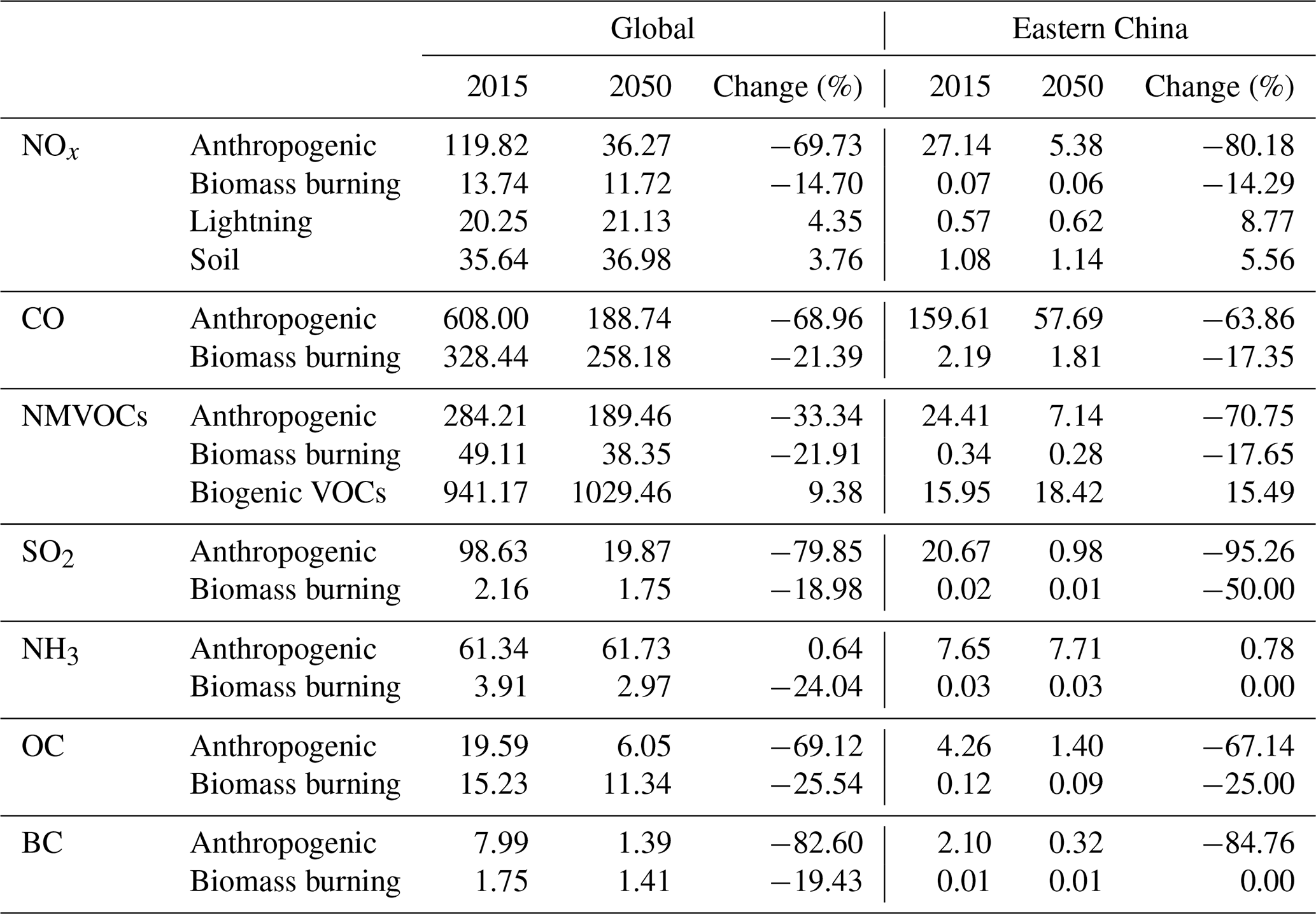
The available emission years of the SSP inventory are 2015, 2020, 2030, 2040, 2050, 2060, 2070, 2080, 2090, and 2100. Therefore, corresponding to the mid-term climate change, we chose 2015 and 2050 emissions to represent the present-day and future emissions, respectively. Present-day (year 2015) and future (year 2050) anthropogenic and biomass burning emissions are given in Table 1. Year 2050 anthropogenic and biomass burning emissions are based on the SSP1-1.9 scenario of CMIP6 experiments. The anthropogenic and biomass burning emissions of NO_x, CO, and non-methane VOCs (NMVOCs) are 27.2, 161.8, and 24.8 Tg yr⁻¹ in EC in 2015, respectively, and are projected to decrease by 80.0 %, 63.2 %, and 70.0 %, respectively, in 2050 relative to 2015. These changes are larger than the decreases in global total emissions (64.1 %, 52.3 %, and 31.6 %, respectively). The anthropogenic emissions of sulfur dioxide (SO₂), organic carbon (OC), and black carbon (BC) are projected to decrease by 95.3 %, 67.1 %, and 84.8 % in EC and by 79.9 %, 69.1 %, and 82.6 % globally, respectively, while ammonia (NH₃) emission remains stable.

Table 1 also lists climate-sensitive natural emissions, including lightning and soil emissions of NO_x and biogenic emissions of VOCs, which are calculated online based on the GCAP 2.0 meteorology. Lightning and soil emissions of NO_x are calculated using the cloud-top height scheme of Price and Rind (1992) and the Berkeley–Dalhousie Soil NO_x Parameterization (BDSNP) scheme developed by Hudman et al. (2012), respectively. Biogenic VOC (BVOC) emissions are computed using the Model of Emissions of Gases and Aerosols from Nature version 2.1 (MEGAN v2.1) (Guenther et al., 2012). In the present day, the lightning and soil emissions of NO_x and biogenic emissions of VOCs are 0.6, 1.1, and 16.0 Tg yr⁻¹, respectively, in EC. Note that VOCs from the biogenic sources (16.0 Tg yr⁻¹) are comparable to those from the anthropogenic emissions (24.4 Tg yr⁻¹) in EC. Compared to 2015, lightning and soil emissions of NO_x and the BVOC emissions are predicted to increase by 8.8 %, 5.6 %, and 15.5 %, respectively, in EC. Changes in all natural emissions are calculated using projected climate change and are considered the effects of climate change.

Table 1 The annual anthropogenic, biomass burning, and natural emissions (Tg yr⁻¹) for the present day (year 2015) and the future (year 2050) under the SSP1-1.9 scenario. The domain of eastern China (EC) is 21.00–45.00° N, 106.25–123.75° E.

2.2.3 Numerical experiments

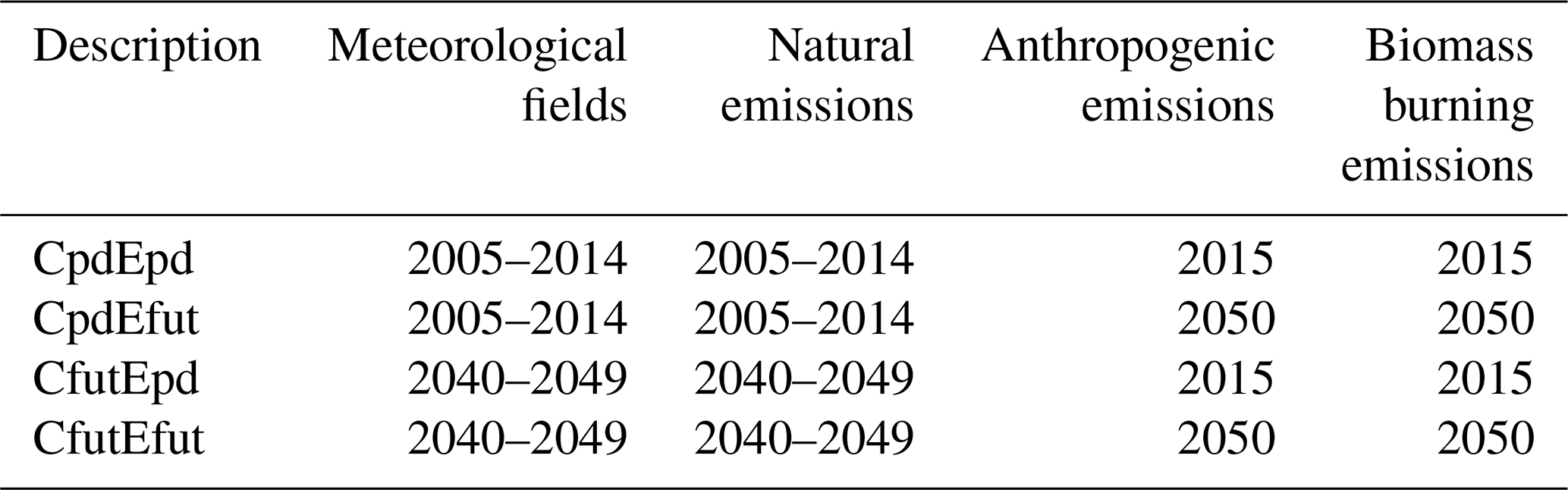
The GCAP 2.0 meteorology is available for four time slices: the pre-industrial era (1851–1860), recent past (2001–2014), near future (2040–2049), and end of the century (2090–2099). Considering the available GCAP 2.0 meteorology, the 2005–2014 meteorology is used to represent the present-day climate (2010), and the 2040–2049 meteorology under the SSP1-1.9 scenario is used to represent the future climate (2045). To examine the respective and combined effects of future changes in climate and emissions on surface O₃ levels, four numerical experiments are set up (Table 2). The simulations of CpdEpd, CpdEfut, CfutEpd, and CfutEfut represent O₃ levels under present-day climate and emissions, present-day climate and future emissions, future climate and present-day emissions, and future climate and emissions, respectively. Therefore, CfutEpd minus CpdEpd or CpdEfut minus CpdEpd indicates the individual effect of climate change or emission change on O₃ concentrations, and CfutEfut minus CpdEpd indicates the combined effect of climate and emission changes. To smooth out the noise of natural climate variabilities, each simulation is conducted for 10 years after a 1-year spin-up. Unless otherwise noted, all the results presented in this study are 10-year averages of 2005–2014 or 2040–2049.

Table 2 Experiment design.

2.3 Statistical analysis methods

2.3.1 Stepwise MLR model and LMG method

To identify meteorological variables that have a significant effect on climate-induced MDA8 O₃ changes, we applied a stepwise multiple linear regression (MLR) model to relate 10-year daily MDA8 O₃ anomalies to 10-year daily meteorological parameter anomalies in the target region or each grid cell. The time series of 10-year daily MDA8 O₃ anomalies are obtained by CfutEpd minus CpdEpd, and 10-year daily meteorological parameter anomalies are obtained by subtracting 2005–2014 from 2040–2049. Nine meteorological variables are considered in the MLR analysis (Table 3), comprising daily maximum 2 m temperature (T2max), relative humidity (RH), surface incoming shortwave radiation (SW), planet boundary layer height (PBLH), precipitation (PREC), sea level pressure (SLP), and 850 hPa wind fields (U850, V850, and WS850). We first correlated 10-year daily MDA8 O₃ anomalies with 10-year daily meteorological parameter anomalies and excluded meteorological variables that did not significantly correlate with MDA8 O₃ at the 95 % confidence level. We then applied collinearity statistics to the retained meteorological variables based on the variance inflation factor (VIF): the meteorological variable with the largest VIF was sequentially excluded until the VIFs of all meteorological variables were less than 10. After these steps, the reserved meteorological variables were read into the stepwise MLR model, which is in the following form (Li et al., 2019):

$$\begin{array}{}\text{(1)}& y={\mathit{\beta }}_{\mathrm{0}}+{\sum }_{k=\mathrm{1}}^N{\mathit{\beta }}_k{x}_k+\text{interaction}\text{term},\end{array}$$

where y is the daily MDA8 O₃ anomalies, (x₁, …, x_N) represents the N meteorological variable screened by the stepwise MLR model, and β_k is the regression coefficient for the kth meteorological variable. The adjusted coefficient of determination (R²_adj) of the MLR equation represents the proportion of climate-induced MDA8 O₃ changes that can be explained by the changes in key meteorological variables.

We then used the Lindeman, Merenda, and Gold (LMG) method (Grömping, 2006) to quantify the relative contribution of each meteorological variable reserved in the MLR equation. The LMG method decomposes the MLR model-explained total R²_adj into the non-negative individual R²_adj contribution from each correlative regressor.

Table 3 Meteorological variables considered in the statistical analysis.

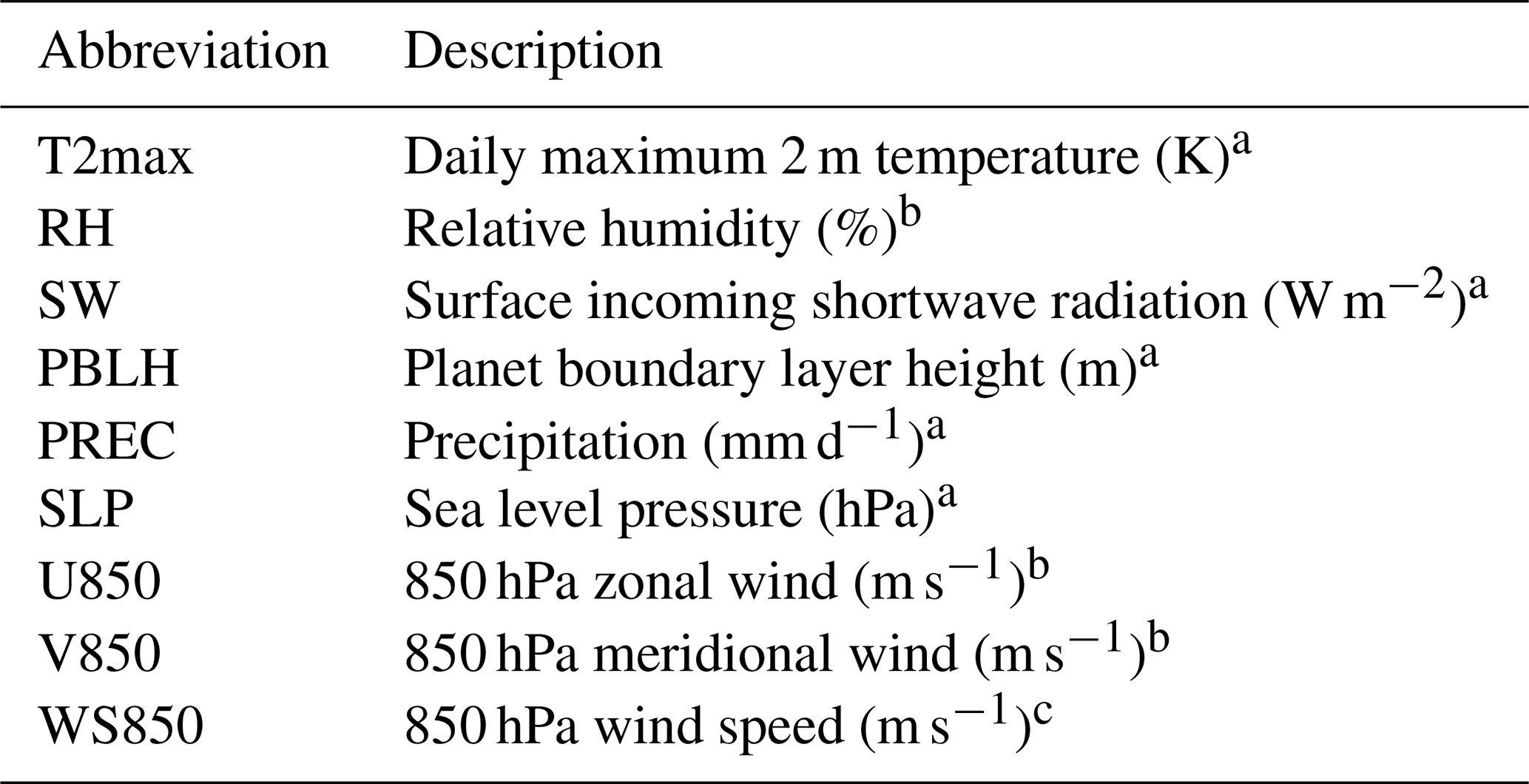
^a Temporal resolution is 1 h. ^b Temporal resolution is 3 h. ^c Calculated from the horizontal wind vectors (U850, V850).

2.3.2 IPR analysis

Integrated process rate (IPR) analysis is used to quantify the contributions of climate-driven change in physical and chemical processes to O₃ mass changes in different seasons in EC (21.00–45.00° N, 106.25–123.75° E). Five processes that influence O₃ levels are investigated, comprising net chemical production, PBL mixing, dry deposition, cloud convection, and horizontal and vertical advection transport, which jointly determine the O₃ mass balance. All of the processes are diagnosed at every time step and then summed over each day. The contribution of each process was calculated following Eqs. (2) and (3) (Dang and Liao, 2019b):

$$\begin{array}{}\text{(2)}& {\displaystyle }{\mathrm{PC}}_{\mathrm{DIFF}\mathit{\_}i}={\mathrm{PC}}_{\mathrm{CfutEpd}\mathit{\_}i}-{\mathrm{PC}}_{\mathrm{CpdEpd}\mathit{\_}i},\text{(3)}& {\displaystyle }\mathit{\%}{\mathrm{PC}}_{\mathrm{DIFF}\mathit{\_}i}={\displaystyle \frac{{\mathrm{PC}}_{\mathrm{DIFF}\mathit{\_}i}}{{\sum }_i^n\mathrm{abs}\left({\mathrm{PC}}_{\mathrm{DIFF}\mathit{\_}i}\right)}}\times \mathrm{100}\mathit{\%},\end{array}$$

where n is the number of processes (n=5); PC_{CpdEpd_i} and PC_{CfutEpd_i} are the seasonal mean O₃ mass by process i from the CpdEpd and CfutEpd simulations, respectively; and PC_{DIFF_i} is the climate-driven change in O₃ mass by process i. %PC_{DIFF_i} is the proportion of process i in the total O₃ mass change caused by all processes. Note that the sum of absolute values of %PC_{DIFF_i} for all processes equals 100 %. The IPR analysis method has been widely used in previous studies to identify the key processes that contribute to air pollution episodes (Gong and Liao, 2019; Dai et al., 2023; Dang and Liao, 2019b) or drive the interannual and decadal variations in air pollutants (Yang et al., 2022; Mu and Liao, 2014).

2.4 CMIP6 data

The projected climate change by GCAP 2.0 may have uncertainties. To identify the range of uncertainties in the effects of climate change on MDA8 O₃, we downloaded multi-model results of monthly means of the meteorological variables consistent with those in Table 3 in the present day (2005–2014) and future (2040–2049) under the SSP1-1.9 scenario from the CMIP6 data repository (https://esgf-node.llnl.gov/search/cmip6/, last access: 22 March 2025). Since only six climate models in CMIP6 can provide PBLH, we selected outputs with the “r1” variant label from these models (Table S1). Note that GISS-E2.1-G and GISS-E2.1-H are coupled models of the GISS-E2.1 atmospheric model with the GISS and HYCOM ocean models, respectively, while GCAP 2.0 (or GISS-E2.1) is the atmosphere-only model with prescribed sea surface temperatures. We extracted the monthly values for 2005–2014 and 2040–2049 from the raw data and interpolated them into GCAP 2.0 resolution (2°×2.5°) by bilinear interpolation.

3 Results

3.1 Projected future climate change over China

3.1.1 Projected climate change over 2010–2045 by GCAP 2.0

Figure 1 shows the projected 2010–2045 changes in seasonal mean T2max, RH, SW, PBLH, PREC, U850 and V850, and SLP in winter (December–January–February, DJF), spring (March–April–May, MAM), summer (June–July–August, JJA), and autumn (September–October–November, SON) over China by GCAP 2.0 (or GISS-E2.1 GCM) under the SSP1-1.9 scenario. The projected T2max, SW, and PBLH generally increase over EC, while RH generally decreases. Regionally, the maximum increases in T2max occur in northeastern China in DJF (2.0–2.5 K). The NCP (green rectangle in Fig. 1) has the largest temperature increases in other seasons, with values of 2.0–2.5 K in MAM, 1.5–2.0 K in JJA, and 1.0–1.5 K in SON. RH has a decrease of 2 %–6 % over northern China in MAM and JJA and of 2 %–4 % over southern China in SON. Changes in SW and PBLH have similar spatial distributions, both of which increase largely over northern China in MAM and JJA. Precipitation generally increases over southeastern China in DJF and SON and decreases in northern China in MAM. With respect to atmospheric circulations, over the northwestern Pacific Ocean, there is anomalous high pressure in DJF and anomalous low pressure in other seasons. As a result, over EC, anomalous southerlies prevail in DJF and anomalous northwesterlies/northerlies prevail in other seasons.

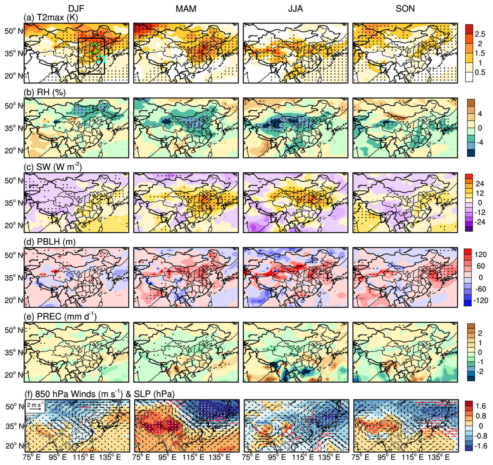
Figure 1 Projected 2010–2045 changes in seasonal mean (a) daily maximum 2 m air temperature (T2max, K), (b) surface relative humidity (RH, %), (c) surface incoming shortwave radiation (SW, W m⁻²), (d) planet boundary layer height (PBLH, m), (e) precipitation (PREC, mm d⁻¹), and (f) wind fields at 850 hPa (arrows, m s⁻¹) and sea level pressure (SLP, shading, hPa) by GCAP 2.0 under the SSP1-1.9 scenario. The dotted areas and red arrows represent a statistically significant difference at 95 % confidence according to Student's two-sample t test. The black, green, and blue rectangles in (a) indicate the domain of eastern China (EC; 21.00–45.00° N, 106.25–123.75° E), the North China Plain (NCP; 35.00–41.00° N, 113.75–118.75° E), and the Yangtze River Delta (YRD; 29.00–33.00° N, 118.75–123.75° E), respectively.

3.1.2 Comparisons with projected climate change from other CMIP6 models

The projected 2010–2045 changes in meteorological parameters (Table 3) under the SSP1-1.9 scenario over EC by GCAP 2.0 are compared with those from six other CMIP6 models in Fig. 2. Increases in T2max, SW, and PBLH throughout the year are robust features among all CMIP6 models. Most models projected reductions in RH and SLP and increases in PREC. However, there are large model differences in winds at 850 hPa with inconsistent signs of changes. On a multi-model mean (MMM) basis, projected annual mean changes over EC in T2max, SW, PBLH, PREC, RH, and SLP are 1.4 K, 11.8 W m⁻², 30.6 m, 0.3 mm d⁻¹, −0.7 %, and −0.3 hPa, respectively. Consistently with the MMM, the GCAP 2.0 projections show overall increases in T2max, SW, PBLH, and PREC and decreases in RH and SLP, with annual mean changes of 1.1 K, 7.3 W m⁻², 23.7 m, 0.03 mm d⁻¹, −1.3 %, and −0.3 hPa, respectively. Therefore, relative to the MMM, GCAP 2.0 underestimates the increases in T2max, SW, PBLH, and PREC and overestimates the decreases in RH. The uncertainties in simulated future O₃ caused by the uncertainties in future climate change will be quantified in Sect. 3.4.

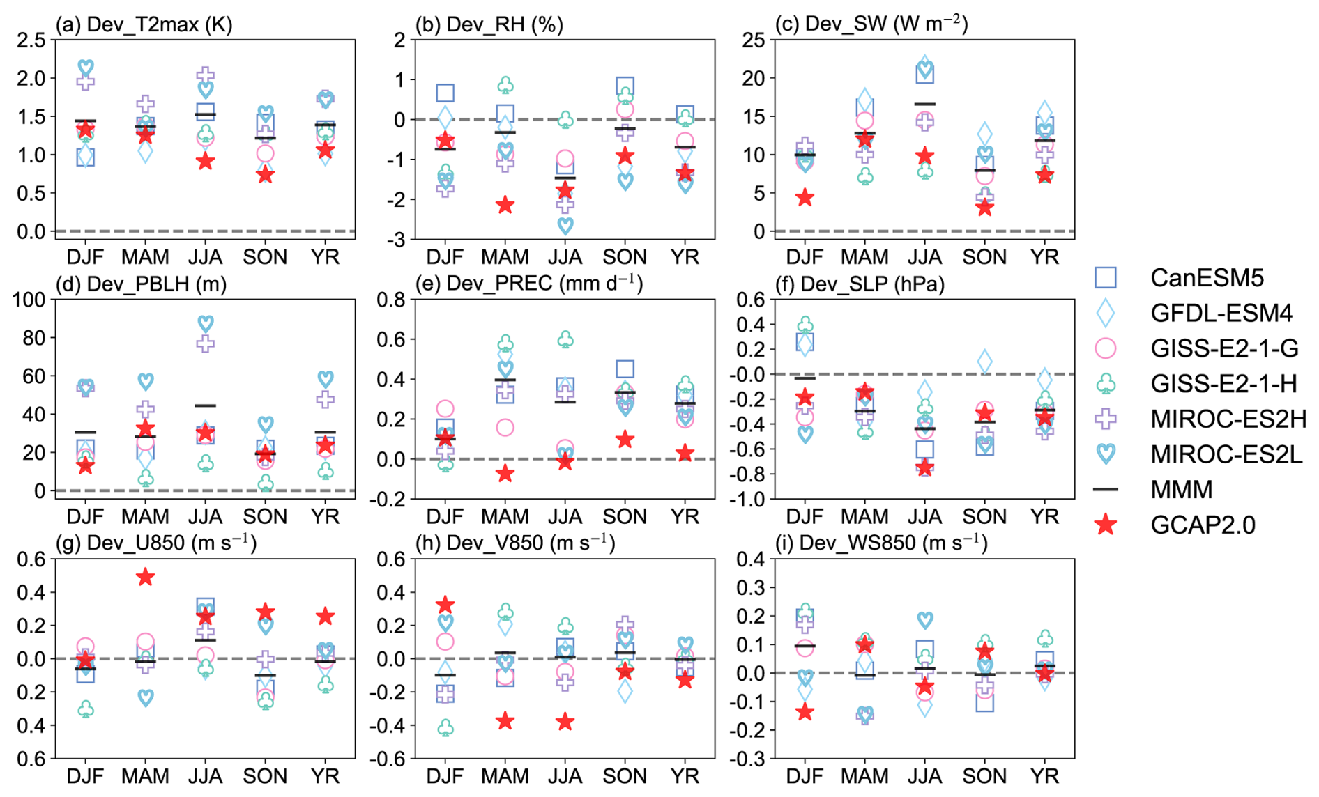
Figure 2 Comparisons of simulated 2010–2045 changes in seasonal and annual mean meteorological parameters over EC by GCAP 2.0 with those by six other CMIP6 models under the SSP1-1.9 scenario. Note that GISS-E2.1-G and GISS-E2.1-H are coupled models of the GISS-E2.1 atmospheric model with the GISS and HYCOM ocean models, respectively, while GCAP 2.0 (or GISS-E2.1) is the atmosphere-only model with prescribed sea surface temperatures. The multi-model mean (MMM) is calculated from the average of the six CMIP6 models. Different markers represent different models, black lines represent MMM, and red stars represent GCAP 2.0 results.

3.2 Simulated present-day and future tropospheric O₃

3.2.1 Present-day tropospheric O₃ and model evaluation

Figure 3 shows simulated present-day MDA8 O₃ concentrations from CpdEpd simulation and the observations in 2015 from CNEMC. We use observations of 2015 to evaluate the simulated present-day MDA8 O₃ concentrations because emissions of the year 2015 are used for the present day. Simulated MDA8 O₃ concentrations in EC are highest in JJA (50–70 ppbv), followed by MAM (35–55 ppbv), SON (30–50 ppbv), and DJF (10–45 ppbv). The model generally captures the spatial distributions of the observed seasonal mean MDA8 O₃ levels over China, with spatial correlation coefficients (R) of 0.63, 0.12, 0.54, and 0.33 in DJF, MAM, JJA, and SON, respectively. Dang and Liao (2019a) also reported a low spatial correlation coefficient (R of 0.08) between observed and simulated seasonal mean O₃ in China in MAM of 2014–2017, which was attributed to the negative biases in NCP and YRD, whereas the positive biases are outside these two regions. The model overestimates MDA8 O₃ concentrations in China, with normalized mean biases (NMBs) of 7.1 %–18.6 % in different seasons. Figure S1 in the Supplement shows monthly variations in simulated and observed MDA8 O₃ levels over EC, NCP, and YRD. Both observed and simulated monthly mean MDA8 O₃ concentrations are high during warm months (April–September) in these three regions. The NMBs in EC, NCP, and YRD are 11.1 %, −12.8 %, and −0.9 %, respectively, which is consistent with results of Dang and Liao (2019a). The scatterplots of model results vs. observations for grids in these three regions show correlation coefficients (R) of 0.76 to 0.94 when all of the data from 2015 are considered.

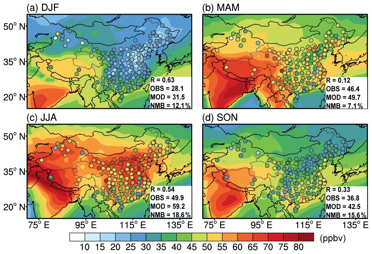
Figure 3 Spatial distributions of observed (CNEMC, circles) and simulated (CpdEpd, shading) seasonal mean MDA8 O₃ concentrations (ppbv) in 2015. Observed (OBS) and simulated (MOD) values averaged over 118 grids and their spatial correlation coefficients (R) and normalized mean biases (NMB) are also shown at the bottom right corner of each panel.

3.2.2 Future changes in tropospheric O₃ driven by climate change

Figure 4a shows future changes in seasonal mean MDA8 O₃ concentrations due to climate change (CfutEpd minus CpdEpd). Climate change alone causes large increases in MDA8 O₃ values over EC in MAM and JJA, with the maximum value reaching 7.6 ppbv in NCP in JJA. In DJF, MAM, JJA, and SON, the regional and seasonal mean MDA8 O₃ values increase by 0.5 (1.5 %), 1.3 (2.7 %), 2.3 (3.9 %), and 0.4 ppbv (1.0 %), respectively, in EC; by 0.4 (2.0 %), 2.8 (6.7 %), 4.7 (7.3 %), and 1.5 ppbv (4.6 %), respectively, in NCP; and by 1.1 (3.5 %), 1.7 (3.3 %), 3.0 (5.1 %), and 0.3 ppbv (0.6 %), respectively, in YRD. Our results are lower than those of the recent study by Bhattarai et al. (2024), who reported that climate change alone could lead to an increase of 5–15 ppbv in JJA MDA8 O₃ levels in EC over 2010–2050 under the SSP1-2.6 scenario using the Community Earth System Model (CESM) and Community Atmospheric Model version 4 with Chemistry (CAM4-chem).

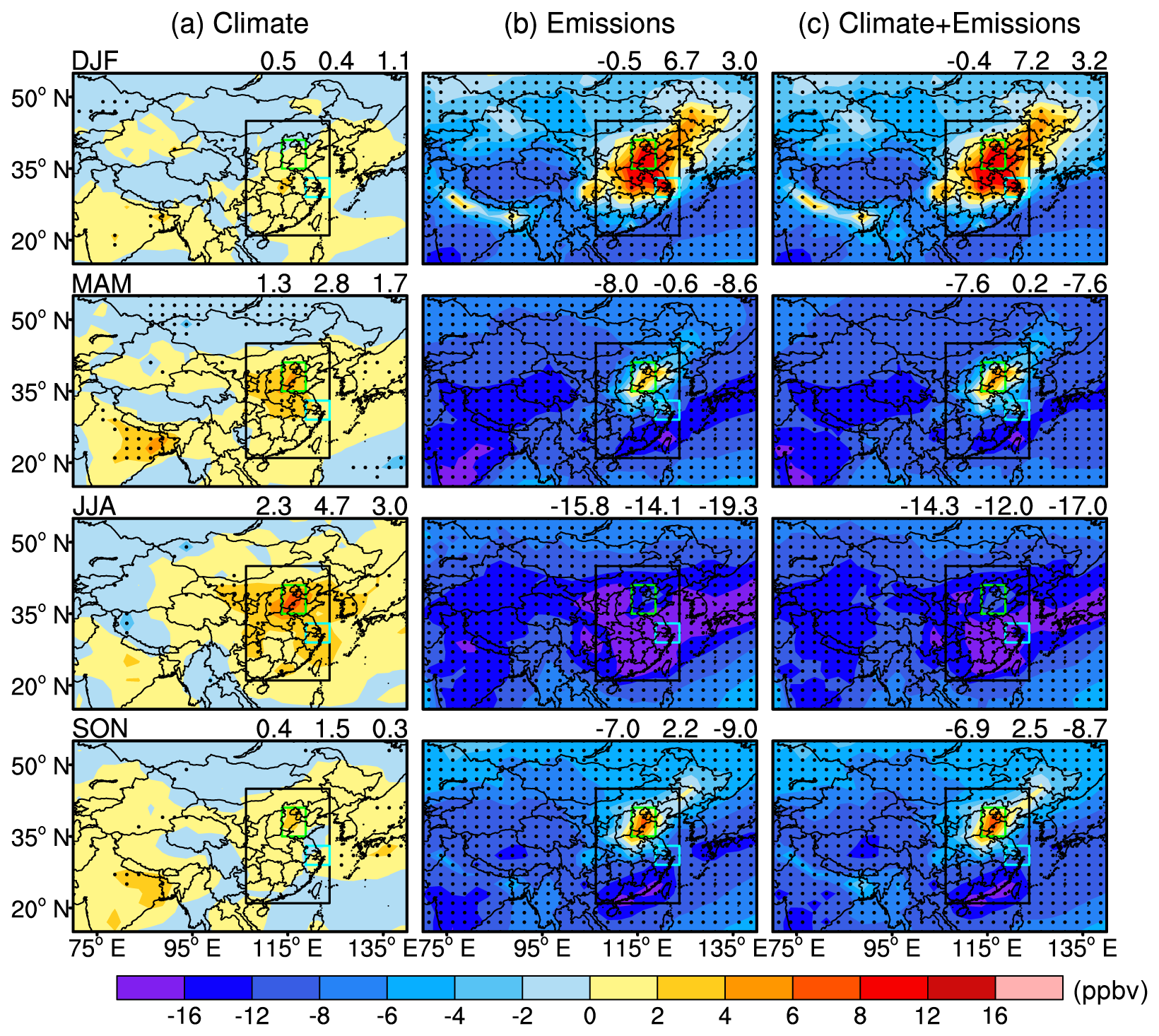
Figure 4 Predicted future changes in seasonal mean MDA8 O₃ concentrations (ppbv) due to (a) climate change alone (CfutEpd minus CpdEpd), (b) emission change alone (CpdEfut minus CpdEpd), and (c) combined climate and emission changes (CfutEfut minus CpdEpd) under the SSP1-1.9 scenario. The black, green, and blue rectangles indicate the domains of EC, NCP, and YRD, respectively. The dotted areas represent a statistically significant difference at the 95 % level according to Student's two-sample t test. The values at the top right of each panel are the regional mean values of EC, NCP, and YRD, respectively.

The pressure–latitude cross sections of climate-driven seasonal mean O₃ changes from the surface to 500 hPa for EC, NCP, and YRD are shown in Fig. 5. Vertically, O₃ increases exceeding 1 ppbv extend from the surface to 500 hPa altitude over the three regions in JJA. The maximum O₃ increases of 4–5 ppbv in NCP occur both at the surface and around 850 hPa, and those of 3–5 ppbv in YRD occur between 930 and 736 hPa. The O₃ increases over EC are large below 700 hPa over 25–41° N, and the location of high values shifts from north to south with altitude, which is dominated by the pattern of NCP. In other seasons, the O₃ increases of 1–3 ppbv are generally near the surface.

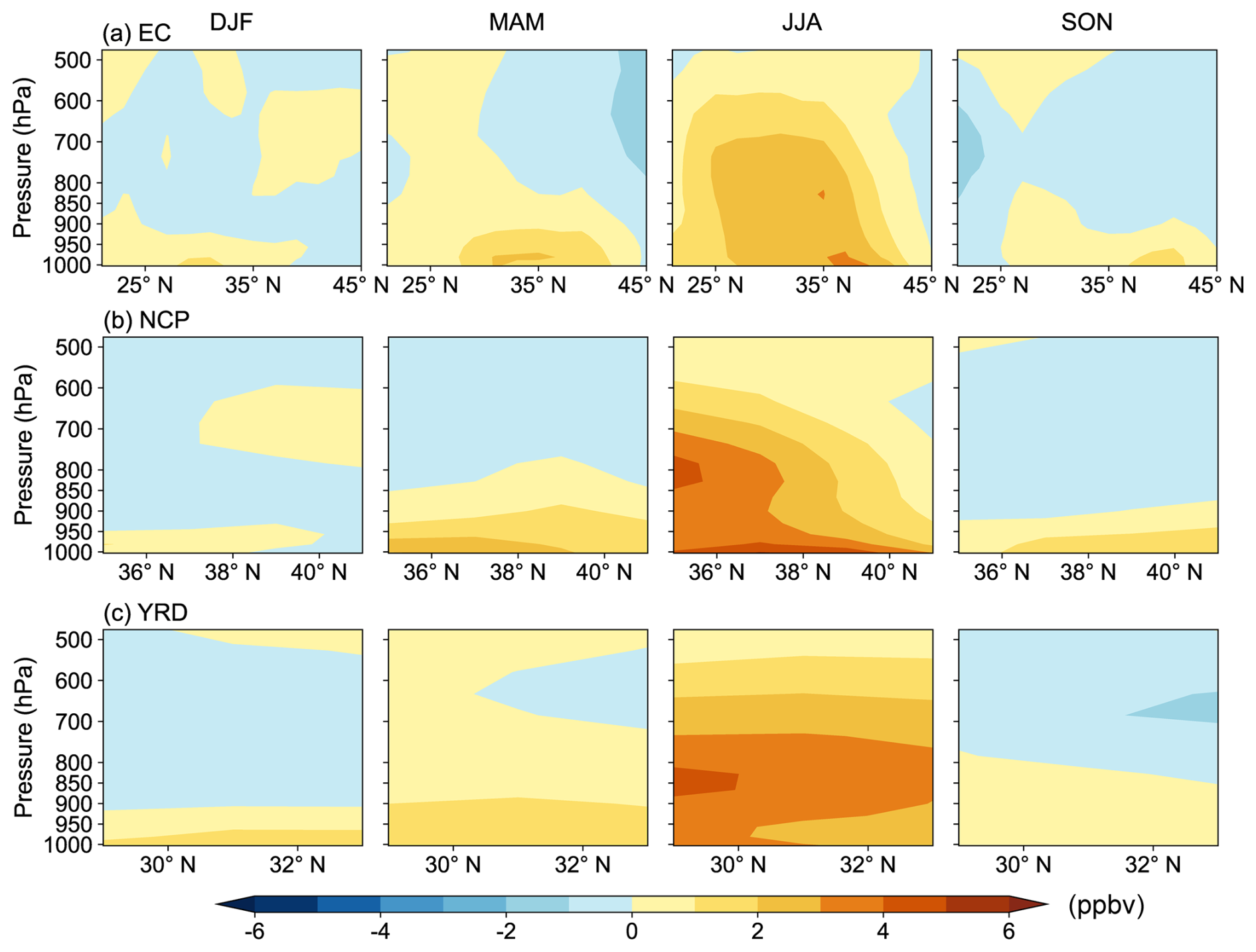
Figure 5 The pressure–latitude cross sections of climate-driven seasonal mean O₃ changes (ppbv) averaged over the longitudes of (a) 106.25–123.75° E for EC, (b) 113.75–118.75° E for NCP, and (c) 118.75–123.75° E for YRD.

3.3 Key meteorological parameters and processes for climate-induced O₃ changes

3.3.1 Key meteorological parameters for climate-induced MDA8 O₃ changes

For climate-induced changes in MDA8 O₃, the stepwise MLR model is used to identify key meteorological variables that have a statistically significant effect on MDA8 O₃, and the obtained R²_adj represents the proportion of climate-induced MDA8 O₃ changes that can be explained by the changes in these key meteorological variables retained in the MLR equation. Then the LMG method is used to decompose the MLR model-explained total R²_adj and get the relative contribution of each meteorological variable.

Table 4 shows the MLR equations between the daily anomalies of MDA8 O₃ and daily anomalies of meteorological variables over EC for each season. The daily anomalies of both MDA8 O₃ and meteorological variables are 10-year daily values, which were derived from CfutEpd minus CpdEpd and 2040–2049 minus 2005–2014, respectively. For each key meteorological variable, the positive or negative regression coefficient represents a statistically significant positive or negative effect of this variable on MDA8 O₃ concentrations. The R²_adj values of the MLR equations are 0.76, 0.74, 0.58, and 0.76 in DJF, MAM, JJA, and SON, respectively, indicating that 76 %, 74 %, 58 %, and 76 % of the climate-induced changes in MDA8 O₃ can be explained by the changes in the key meteorological variables retained in MLR equations. Figure 6 shows the LMG-decomposed contribution of each key meteorological variable in fitting climate-driven MDA8 O₃ changes over EC. The three most important meteorological variables are T2max, SW, and RH, with total contributions of 71.2 % (T2max + SW + RH) in DJF, 78.2 % (T2max + SW + RH) in MAM, 70.1 % (SW + RH + T2max) in JJA, and 49.9 % (T2max + RH) in SON. PBLH is also a major meteorological variable, with contributions of 9.6 %–24.5 % in different seasons. The total contributions of the circulation changes are 13.4 % (SLP + WS850 + V850), 9.8 % (V850 + U850), 11.4 % (WS850 + V850 + SLP), and 9.5 % (SLP + V850 + WS850) in DJF, MAM, JJA, and SON, respectively.

Table 4 Stepwise multiple linear regression (MLR) equations between the daily anomalies of MDA8 O₃ (CfutEpd minus CpdEpd) and daily anomalies of meteorological parameters (2040–2049 minus 2005–2014) in EC. All the regression coefficients shown in the equations passed the t test of significance at the 0.05 level.

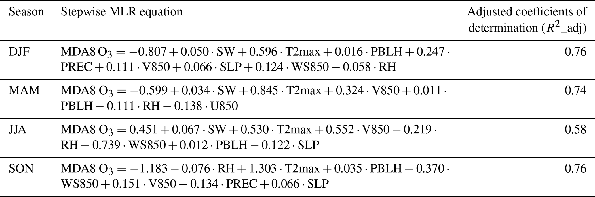
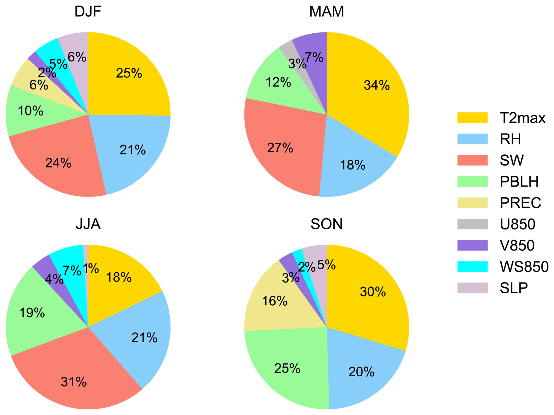
Figure 6 The LMG-decomposed contribution (%) of each meteorological variable screened by the stepwise MLR model in fitting climate-driven MDA8 O₃ changes over EC. See Table 3 for the meanings of the abbreviations of meteorological variables.

Large-scale regional averages could obscure local characteristics, so we further conducted MLR and LMG analysis on each grid cell to identify the first and second most important meteorological parameters (hereafter called “1st MET” and “2nd MET”) in China as shown in Fig. 7. In DJF, the 1st MET is T2max in southern EC and is SW or PBLH in northern EC, which has relative contributions of 30 %–70 % from LMG analyses. In JJA, the 1st MET is T2max in most parts of northern EC (north of 36° N); SW in most parts of central EC (26–36° N), Beijing, and Tianjin; and RH and WS850 in southern EC (south of 26° N). In the corresponding areas, T2max and SW have relative contributions of 30 %–70 % and RH has relative contributions of 10 %–30 %. The regional heterogeneity of the 2nd MET increases compared to the 1st MET. In DJF, the 2nd MET is RH in northern EC and SW in southern EC, with relative contributions of 10 %–30 %. In JJA, the 2nd MET is mainly SW or T2max in northern EC and RH or WS850 in southern EC. The relative contribution of the 2nd MET (SW or T2max) in central EC can be 30 %–50 % in JJA. In summary, the key meteorological parameters for climate-induced MDA8 O₃ changes are not only temperature, but also SW, RH, and PBLH, depending on locations and seasons.

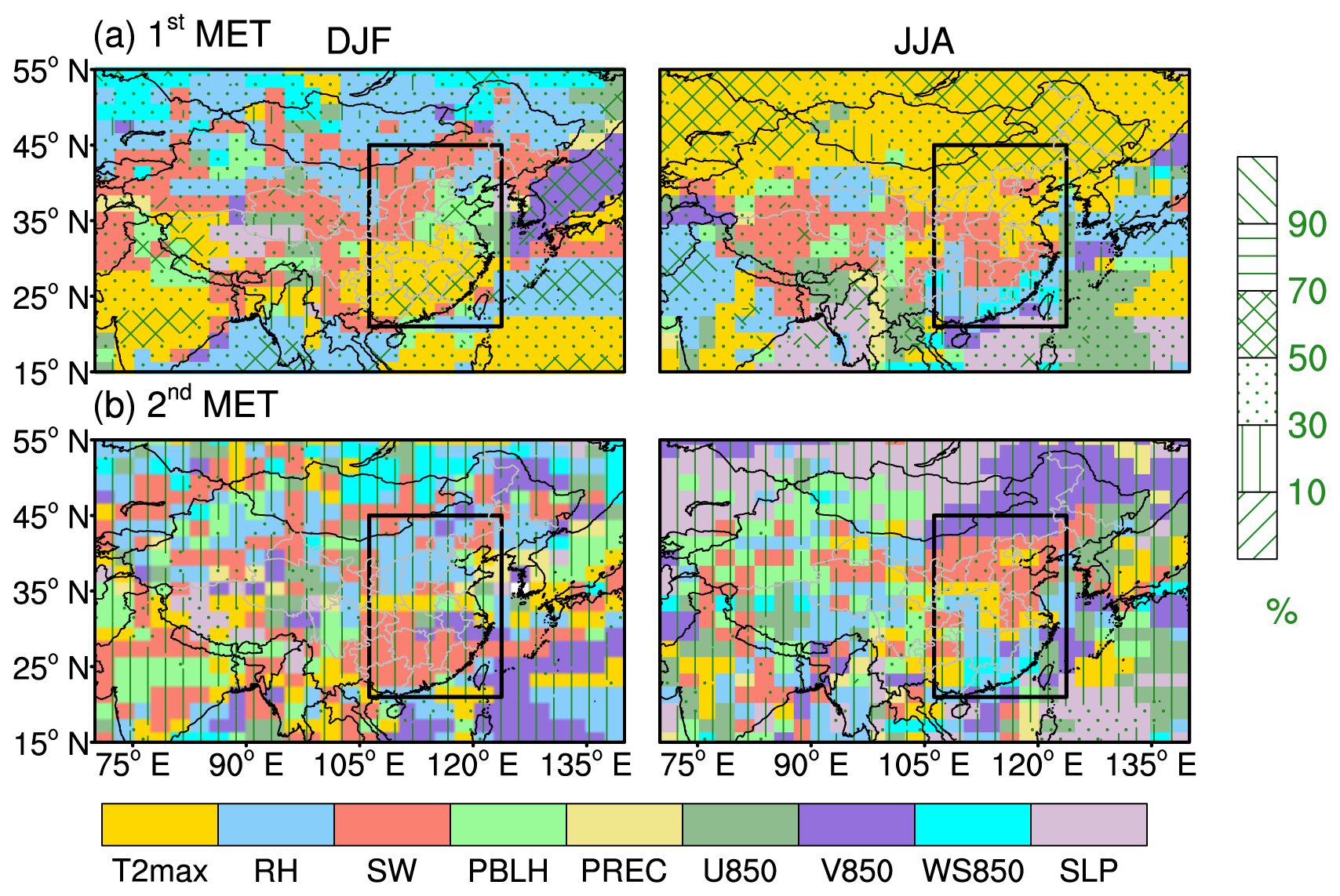
Figure 7 The (a) first and (b) second most important meteorological parameters (1st MET and 2nd MET, respectively) for climate-induced MDA8 O₃ changes in China and their relative contributions in DJF and JJA., All 1st MET and 2nd MET results in each 2°×2.5° grid cell are statistically significantly correlated with MDA8 O₃ (p<0.05). The overlaid fill patterns represent the relative contribution of the meteorological variable on this grid.

3.3.2 Key processes for climate-induced O₃ changes

We performed IPR analysis to understand the intrinsic mechanism of the impact of climate change on O₃ in EC. Figure 8 shows the vertical profiles of present-day seasonal mean O₃ mass and climate-driven O₃ mass changes in five processes (net chemical production, PBL mixing, dry deposition, cloud convection, and horizontal and vertical advection transport) in EC. Since surface O₃ concentrations are determined by the processes within the boundary layer (Gong and Liao, 2019), in Table 5 we also listed the present-day O₃ budget of five processes in EC within the boundary layer and the climate-driven O₃ budget changes by each process.

In the present day (Fig. 8a), net chemical production is negative at the surface due to the O₃ titration effect by abundant NO_x and is positive in the upper levels due to the decreases in NO_x concentrations and the strong solar radiation (Gong and Liao, 2019). PBL mixing refers to O₃ mass fluxes by turbulence within the boundary layer, which transports O₃ based on the concentration gradient. Since O₃ concentrations are higher in the upper boundary layers than at the surface (Fig. S2), PBL mixing leads to decreases in O₃ in upper layers (950 to 800 hPa) and increases in surface-layer O₃ levels. Dry deposition occurs only at the surface, with the values of −122.1 to −37.5 Gg d⁻¹ in different seasons. The cloud convection process in the GEOS-Chem model describes the redistribution of species concentrations due to upward convection inside the cumulus and subsidence outside the cumulus. Cloud convection has a large positive value below 950 hPa in all seasons due to the frequent non-precipitation shallow convection in GISS-E2.1 (Wu et al., 2007; Miller et al., 2021) and higher O₃ concentrations above 950 hPa. Horizontal and vertical advection below 850 hPa is positive in DJF and negative in other seasons. For the present-day O₃ budget within the boundary layer (Table 5, PC_CpdEpd), net chemical production is the dominant process that contributes to the O₃ budget in JJA, MAM, and SON, with values of 136.3, 56.5, and 37.6 Gg d⁻¹, respectively. Cloud convection has contributions of 11.0–34.4 Gg d⁻¹ to the O₃ budget. The horizontal and vertical advection is 0.4 Gg d⁻¹ in DJF and −23.8 to −2.7 Gg d⁻¹ in other seasons.

Under the impact of climate change (Fig. 8b), net chemical production exhibits distinct increases below 850 hPa in all seasons, especially in MAM and JJA. Increases in T2max and SW (Fig. 1a and c) result in increases in BVOC emission rates by 0.4 × 10⁻¹¹–2.9 × 10⁻¹¹ kg m⁻² s⁻¹ (Fig. S3) and in photochemical reaction rates, while decreases in RH (Fig. 1b) result in decreases in O₃ destruction (Gong and Liao, 2019), which together promote the net chemical production of O₃. An increase in surface O₃ mass by PBL mixing indicates that more O₃ enters the boundary layer and mixes to the surface as a result of increased PBLH (Fig. 1d). The importance of the chemical process and PBL mixing corresponds well to the 1st MET and 2nd MET shown in Fig. 7. Dry deposition removes more O₃ due to the increases in the net chemical production of O₃. Cloud convection increases near-surface O₃ mass in DJF and MAM but decreases that in JJA. Changes in horizontal and vertical advection reduce O₃ mass in EC at layers below 850 hPa. Anomalous low pressure over EC in DJF indicates the presence of anomalous upward advection (Fig. 1f). Anomalous northwesterlies over northern China in other seasons obstruct the northward transport of BVOCs from southern China and promote the outflow of O₃ and its precursors from EC. Circulation changes have an important effect on JJA O₃ concentrations, which are also confirmed by the 1st MET and 2nd MET (RH or WS850) in southern EC (Fig. 7).

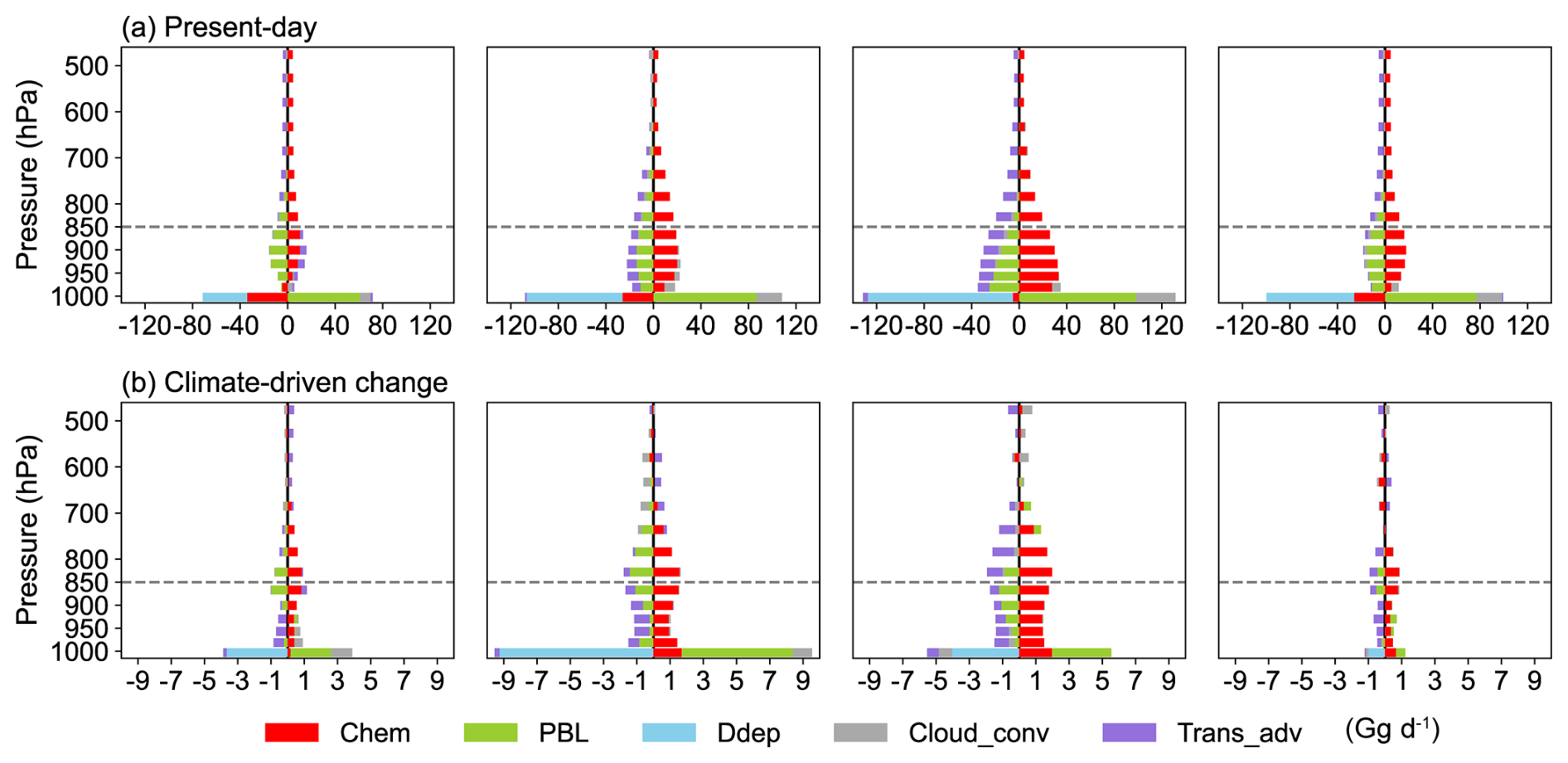
Figure 8 (a) The vertical profile of seasonal mean O₃ mass (Gg d⁻¹) by five processes (bottom axis: net chemical production (Chem), PBL mixing (PBL), dry deposition (Ddep), cloud convection (Cloud_conv), and horizontal and vertical advection (Trans_adv)) over EC in the present day (CpdEpd) and (b) the climate-driven changes in seasonal mean O₃ mass of each process (CfutEpd minus CpdEpd). All the panels have the same vertical axis in hectopascals (hPa).

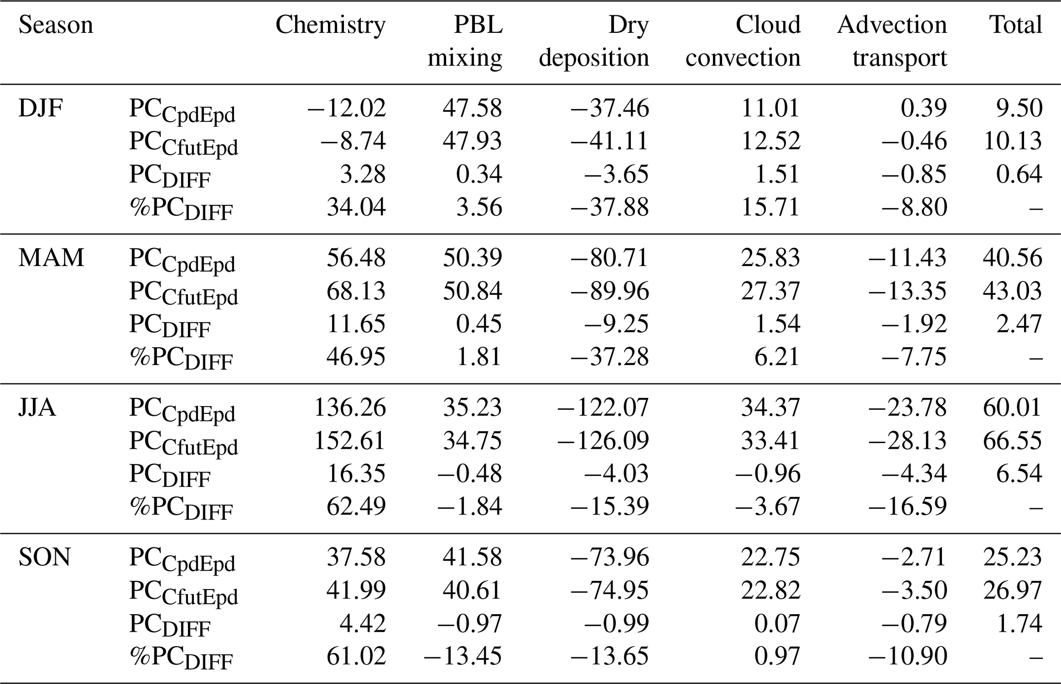
The sums of the climate-driven O₃ mass changes by all processes in EC are 0.6, 2.5, 6.5, and 1.7 Gg d⁻¹ in DJF, MAM, JJA, and SON, respectively (Table 5, PC_DIFF), which are consistent with the seasonal variations in climate-induced MDA8 O₃ (Fig. 4). The net chemical production, dry deposition, and horizontal and vertical advection change by 3.3 to 16.4, −9.3 to −1.0, and −4.3 to −0.8 Gg d⁻¹, respectively, in different seasons. The cloud convection increases by 1.5 Gg d⁻¹ in DJF and MAM and decreases by 1.0 Gg d⁻¹ in JJA. Considering the relative contributions of individual processes (Table 5, %PC_DIFF), net chemical production is the most important process contributing to the increases in O₃ mass in all seasons, with a relative contribution of 34.0 %–62.5 %. Horizontal and vertical advection in JJA (−16.6 %) or dry deposition in other seasons (−37.9 % to −13.7 %) is the major process that reduces O₃ mass as the O₃ mass increases from chemical reactions.

Table 5 Seasonal mean O₃ budgets (Gg d⁻¹) within the boundary layer over EC in CpdEpd (PC_CpdEpd) and CfutEpd (PC_CfutEpd). The climate-driven O₃ budget changes in five processes (PC_DIFF) and the relative contribution of each process to the total O₃ mass changes (%PC_DIFF, %) are also listed, following Eqs. (2) and (3) in Sect. 2.3.2.

3.4 Projections of climate-driven MDA8 O₃ changes from the CMIP6 models

In Sect. 3.3.1, we describe how we applied the stepwise MLR model to relate 10-year daily MDA8 O₃ anomalies to 10-year daily meteorological parameter anomalies at each grid cell and obtained the corresponding MLR equation. The climate-driven seasonal mean MDA8 O₃ concentration changes projected by the stepwise MLR model at each grid cell can be obtained by substituting the corresponding seasonal mean meteorological parameter anomalies of GCAP 2.0 into the regression equations obtained by the daily anomalies above, which will be referred to as Dev_MLR_MDA8 hereafter. The Dev_MLR_MDA8 values for a target region are then obtained by averaging over all the grid cells in the region. We selected EC, NCP, and YRD as the target regions in this study. Figure 9a–c evaluate the seasonal and annual mean Dev_MLR_MDA8 values averaged over EC, NCP, and YRD by comparing them with the simulated values by GCAP 2.0 (hereafter called Dev_GCAP2_MDA8). The seasonal and annual mean values of Dev_MLR_MDA8 and Dev_GCAP2_MDA8 are exactly the same, with an R value of 1.0 and NMB value of 0.0 % in all three regions. In China, the spatial distributions and magnitudes of the seasonal mean Dev_MLR_MDA8 values are consistent with the seasonal mean Dev_GCAP2_MDA8 values (Fig. S4), with high pattern correlation coefficients of 1.0 in four seasons, indicating that it is feasible to predict climate-driven MDA8 O₃ concentration changes by the stepwise MLR model. Therefore, we input the corresponding seasonal mean meteorological parameter anomalies from the six CMIP6 models into the regression equations to obtain multi-model projections of climate-induced MDA8 O₃ changes under a carbon neutrality scenario.

Figures 9d–f show the climate-driven seasonal and annual mean MDA8 O₃ changes averaged over the EC, NCP, and YRD regions predicted by the stepwise MLR model using meteorology anomalies from GCAP 2.0 and the six other CMIP6 models under the SSP1-1.9 scenario. The Dev_MLR_MDA8 values of GCAP 2.0 and all six CMIP6 models are positive throughout the year in all three regions, indicating that climate change will increase MDA8 O₃ concentrations over polluted regions in China even under a carbon neutrality scenario. Similarly to the GCAP 2.0 results, the Dev_MLR_MDA8 values of all six CMIP6 models in the three regions are much larger in JJA than in other seasons, with the values in the range of 2.9–4.2, 6.5–9.4, and 3.3–8.5 ppbv in EC, NCP, and YRD, respectively. In JJA, the Dev_MLR_MDA8 values of MMM (average of six CMIP6 models) are 3.5, 7.5, and 5.1 ppbv in EC, NCP, and YRD, respectively, higher than the Dev_MLR_MDA8 values of GCAP 2.0 of 2.3, 4.7, and 3.0 pbbv, respectively. In other seasons, the Dev_MLR_MDA8 values of MMM are in the range of 0.9–1.4, 1.2–2.3, and 1.2–2.2 ppbv in EC, NCP, and YRD, respectively, and the Dev_MLR_MDA8 values of GCAP 2.0 are in the range of 0.4–1.3, 0.4–2.8, and 0.3–1.7 pbbv, respectively. Overall, the Dev_MLR_MDA8 values of GCAP 2.0 tend to be at the lower end of the multi-model projection results, especially in JJA. The spatial distributions of climate-driven changes in annual mean MDA8 O₃ concentrations from GCAP 2.0 and the six other CMIP6 models are shown in Fig. S5. The climate-induced increases in annual mean MDA8 O₃ predicted by all models are mainly concentrated in central and northern EC. In NCP and its surrounding areas, while the maximum increases in annual mean MDA8 O₃ concentrations were simulated to be 2–4 ppbv from GCAP 2.0, the values were 4–8 ppbv from four of the six CMIP6 models.

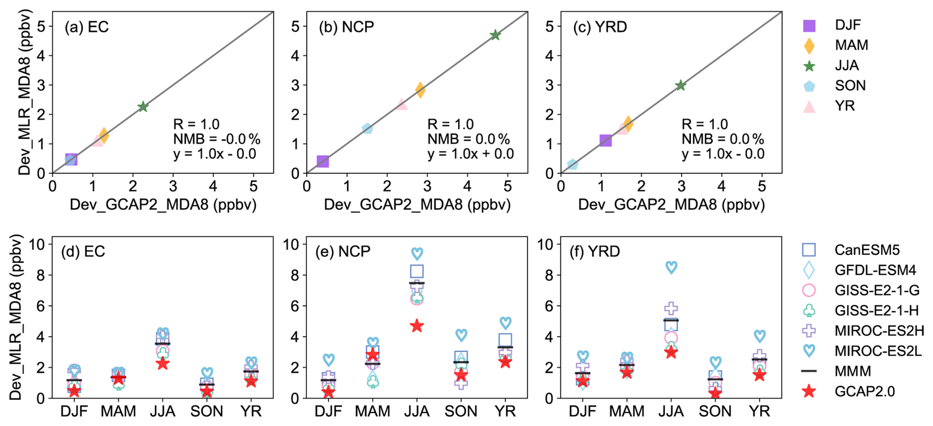
Figure 9 (a–c) Scatterplots of climate-induced MDA8 O₃ changes (ppbv) simulated by GCAP 2.0 (Dev_GCAP2_MDA8) versus those projected by the MLR model (Dev_MLR_MDA8) in the EC, NCP, and YRD regions. The correlation coefficient (R), normalized mean biases (NMB), and linear fit (solid grey line and equation) are also shown. (d–f) The climate-driven seasonal and annual mean MDA8 O₃ concentration changes (ppbv) projected by the MLR model using the climate outputs from GCAP 2.0 and six CMIP6 models under the SSP1-1.9 scenario. The multi-model mean (MMM) is calculated from the average of the six CMIP6 models. Different markers represent different models, black lines represent MMM, and red stars represent GCAP 2.0 results.

3.5 Future changes in tropospheric O₃ driven by changes in anthropogenic emissions

We have shown the large impact of climate change on tropospheric O₃ in previous sections, so it is of interest to briefly examine the effects of emission changes on surface O₃ levels (CpdEfut minus CpdEpd) under a carbon neutrality scenario as shown in Fig. 4b. Emission change alone leads to decreases in MDA8 O₃ concentrations of 0.5 (1.6 %), 8.0 (16.7 %), 15.8 (27.1 %), and 7.0 ppbv (16.5 %) over EC in DJF, MAM, JJA, and SON, respectively. Although the regional mean MDA8 O₃ concentrations in EC decrease in all seasons, the nationwide decreases in MDA8 O₃ concentration occur only in JJA. In other seasons, MDA8 O₃ concentrations in northern China increase owing to changes in anthropogenic emissions, with maximum increases of 8–12 ppbv in DJF. The regional mean MDA8 O₃ concentrations in NCP increase by 6.7 (34.3 %) in DJF and 2.2 ppbv (6.7 %) in SON, and those in YRD increase by 3.0 ppbv (9.5 %) in DJF.

The increases in MDA8 O₃ concentrations by changes in anthropogenic emissions under the carbon neutrality scenario can be explained by the O₃ formation regime. Figure 10 shows the present-day seasonal mean formaldehyde : nitrogen ratio (FNR), which was introduced by Jin and Holloway (2015) to show O₃ sensitivity to its precursors (see Sect. S1 in the Supplement). In DJF, FNR values in eastern China are lower than 1, indicating a general VOC-limited regime. In MAM and SON, the VOC-limited regime shrinks toward northern China, and southern China is in a NO_x-limited (FNR values exceeding 2) or transitional (FNR values between 1 and 2) regime. In JJA, most of China is in a NO_x-limited regime, while the NCP region is still in the VOC-limited or transitional regime. Although the anthropogenic emissions of VOCs and NO_x in NCP decrease significantly (70 %–90 %) under the SSP1-1.9 scenario (Fig. S6), MDA8 O₃ concentrations in this region increase in the future in DJF, MAM, and SON because NCP is in a VOC-limited regime.

Overall, considering the combined effects of climate change and emission change (CfutEfut minus CpdEpd) (Fig. 4c), the spatial distributions and magnitudes of MDA8 O₃ changes are similar to those considering the emission changes alone (Fig. 4b), indicating that future MDA8 O₃ concentrations are dominated by emission changes. However, the effects of the climate penalty (0.5–2.3, 0.4–4.7, and 0.3–3.0 ppbv in EC, NCP, and YRD, respectively) cannot be ignored. Note that the sum of the individual effects of climate (Fig. 4a) and emissions (Fig. 4b) is not equal to the combined effects (Fig. 4c) due to the nonlinear relationship between the simulations (Dang et al., 2021). Additionally, it is worth noting that changes in both climate and emissions lead to increases in MDA8 O₃ in DJF and SON over NCP and in DJF over YRD, calling for more attention to be paid to these regions in future O₃ pollution control strategies.

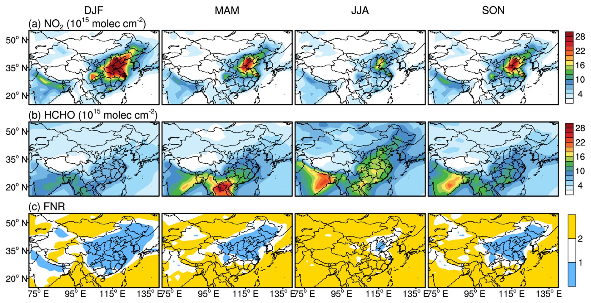
Figure 10 Distributions of seasonal mean tropospheric columns of (a) nitrogen dioxide (NO₂) and (b) formaldehyde (HCHO) (10¹⁵ molec. cm⁻²) and (c) the formaldehyde : nitrogen ratio (FNR) in the present day.

4 Conclusions

In this study, we quantify the effects of climate changes over 2010–2045 on O₃ levels in China under a carbon neutrality scenario (SSP1-1.9 scenario), focusing on the key meteorological parameters and processes for understanding the climate-induced O₃ changes using GCAP 2.0, the stepwise MLR model, the LMG method, and IPR analysis. The uncertainties in future O₃ levels resulting from the uncertainties in the simulated future climate are also quantified using outputs of climate from CMIP6 models.

Under the carbon neutrality scenario, over EC, GCAP 2.0 and all six CMIP6 models project increases in T2max, SW, and PBLH in all seasons and most models project reductions in RH and SLP and increases in PREC. Projected annual mean changes over EC in T2max, SW, PBLH, PREC, RH, and SLP are 1.4 K, 11.8 W m⁻², 30.6 m, 0.3 mm d⁻¹, −0.7 %, and −0.3 hPa, respectively, on a multi-model mean (MMM) basis and 1.1 K, 7.3 W m⁻², 23.7 m, 0.03 mm d⁻¹, −1.3 %, and −0.3 hPa, respectively, from GCAP 2.0. Relative to MMM, GCAP 2.0 underestimates the increases in T2max, SW, PBLH, and PREC and overestimates the decreases in RH.

The GCAP 2.0 model generally reproduces the spatial distribution and magnitude of observed seasonal mean MDA8 O₃ concentrations, with R values of 0.12–0.63 and NMB values of 7.1 %–18.6 % in different seasons. Climate change over 2010–2045 under the carbon neutrality scenario is simulated by GCAP 2.0 to increase the regional mean MDA8 O₃ concentrations by 0.4–2.3 ppbv (1.0 %–3.9 %) over EC, 0.4–4.7 ppbv (2.0 %–7.3 %) over NCP, and 0.3–3.0 ppbv (0.6 %–5.1 %) over YRD in different seasons, with the maximum increases in JJA. Using the stepwise MLR model, we find that changes in the key meteorological variables retained in MLR equations can explain 58 %–76 % of the climate-driven MDA8 O₃ concentration changes over EC. Using the LMG method, we find that the most important meteorological parameters for climate-induced MDA8 O₃ changes are not only temperature, but also SW, RH, and PBLH, depending on locations and seasons. Corresponding to these changes in meteorological parameters, IPR analysis shows that net chemical production (accounting for 34.0 %–62.5 % of total O₃ mass change caused by all processes within the boundary layer) is the most important process contributing to the climate-induced increases in O₃ mass in all seasons. Horizontal and vertical advection in JJA (−16.6 %) or dry deposition in other seasons (−37.9 % to −13.7 %) is the major process that reduces O₃ mass.

Under the carbon neutrality scenario, future MDA8 O₃ concentration changes in EC are dominated by changes in anthropogenic emissions (decrease by 0.5–15.8 ppbv); however, the effects of the climate penalty (increase by 0.5–2.3 ppbv from GCAP 2.0) cannot be ignored. Both climate changes and emission changes increase MDA8 O₃ values in DJF and SON over NCP and in DJF over YRD, indicating that these regions require more attention in future O₃ pollution control.

The estimate of the effect of climate change on O₃ pollution using a single model, GCAP 2.0, may have uncertainties. Therefore, we also obtain the multi-model projection results of future MDA8 O₃ changes driven by 2010–2045 climate change under a carbon neutrality scenario using the stepwise MLR model. In JJA, six CMIP6 models project increases in MDA8 O₃ with values of 2.9–4.2, 6.5–9.4, and 3.3–8.5 ppbv in EC, NCP, and YRD, respectively, indicating that GCAP 2.0 results (2.3, 4.7, and 3.0 pbbv) are at the lower end of the multi-model projections. Additionally, MDA8 O₃ concentrations increase by changes in anthropogenic emissions in the future in DJF, MAM, and SON despite the large reductions in NO_x and VOCs (70 %–90 %) in northern China (Fig. S6) under the SSP1-1.9 scenario, indicating an urgent need to find appropriate emission reduction ratios of VOCs and NO_x based on O₃ sensitivity to precursors and to climate for effective future O₃ pollution control in China.