Technical note: Evolution of convective boundary layer height estimated by Ka-band continuous millimeter wave radar at Wuhan in central China

Using the vertical velocity (w) observed by a Ka-band millimeter wave cloud radar (MMCR) at Wuhan, we investigate the evolution of the convective boundary layer height (CBLH) based on a specified threshold of vertical velocity variance (${\mathit{\sigma }}_{\mathrm{w}}^{\mathrm{2}}$). The CBLHs from the MMCR w in the selected durations are compared with those estimated by the lidar range-corrected signal (RCS) and radiosonde temperature based on different algorithms, showing good agreement with each other. Although these algorithms are based on different dynamic and thermodynamic effects, the diurnal evolution of the CBLH from MMCR is generally consistent with that from lidar, except for a few hours post-sunrise and pre-sunset due to the influence of the aerosol residual layer on the lidar RCS. Meanwhile, the CBLH from MMCR shows less variation with the occurrence of sand and dust and a swifter response for thick clouds relative to that from lidar. In this case, ${\mathit{\sigma }}_{\mathrm{w}}^{\mathrm{2}}$ of the MMCR w identifies the CBLH based on a dynamic effect, which can accurately capture the diurnal evolution of the CBLH compared with that from the change in long-time-mixing aerosol concentration. The monthly and seasonal features of the CBLH at Wuhan are revealed via the MMCR measurement. Hence, considering that the MMCR is capable of continuous observation in various weather conditions, the MMCR w with high resolution can be applied for monitoring the evolution of the CBLH in different atmospheric conditions, which is helpful for improving our comprehensive understanding of the convective boundary layer (CBL) and dynamic processes in the CBL.

1 Introduction

The planetary boundary layer (PBL) is located in the lower part of the troposphere, and this is where the air–land (or air–sea) interaction takes place; thus, the PBL is directly impacted by the surface forcings (Stull, 1988). Owing to the combined effects of friction, evaporation and transpiration, heat transfer, and pollutant emission, the PBL is characterized by complex dynamical processes, with the prominent turbulence features of vorticity and compressibility (Bernardini et al., 2012; Schneider, 2008). The height of the PBL varies with local time, ranging generally from a few tens of meters to a few kilometers at midlatitudes. Since the PBL regulates the exchange of momentum, moisture, and mass between the ground and the free atmosphere (Mahrt, 1999; Holtslag and Nieuwstadt, 1986), the structure of the PBL is an important input variable in numerical weather prediction and climate models (Edwards et al., 2020).

The convective boundary layer (CBL) is a type of PBL driven primarily by convection, and the CBL height (CBLH) has a distinct daily cycle. Convective sources include heat transfer from the ground surface warmed by solar radiation and radiative cooling-induced air sinking from the cloud top; thus, the evolution of CBL is mainly dominated by surface sensible heat, which is significantly influenced by weather conditions, such as clouds and humidity near the surface (Kwon et al., 2022; Ribeiro et al., 2018; Zhang et al. 2014). On a clear day, the CBLH rises after sunrise and reaches its maximum in the afternoon (LeMone et al., 2010; Grossman et al., 2005; Yates et al., 2001). When the CBL collapses after sunset, most of the aerosol particles within the CBL are deposited into the nocturnal stable PBL due to the rapid weakening of convectively driven turbulence, and some particles are transformed into an aerosol residual layer. The residual layer descends gradually due to the sinking effect until it is mixed with the CBL driven by the next day's post-sunrise convection (Blay-Carreras et al., 2014; Heus et al., 2010; Tennekes and Driedonks, 1981). At the CBL top, moisture, aerosols, and other chemical substances can be entrained to the free atmosphere, leading to an entrainment transition zone between the CBL and the free atmosphere (Franck et al., 2021; Liu et al., 2021; Brooks and Fowler, 2007). Hence, the CBL has an influence not only on the dispersion of surface emissions and pollutants (Kong and Yi, 2015; Pal et al., 2015; Stull, 1988), but also on the weather processes above it through the entrainment process (Guo et al., 2017; Brooks and Fowler, 2007; Neggers et al., 2004).

The observations of in situ radiosonde and remote sensing are extensively used to estimate the CBLH and its seasonal features. The radiosonde method can obtain high-precision meteorological parameters, such as temperature, humidity, horizontal wind, and pressure, providing the possibility of estimating CBLH through various algorithms (Seidel et al., 2010; Seibert, 2000). Typically, the vertical gradients of potential temperature and water vapor (including relative humidity and specific humidity) are used to determine the CBLH (Zhang et al., 2022; Guo et al., 2021; Dang et al., 2019; Liu and Liang, 2010; Seidel et al., 2010). Additionally, the CBL top can be evaluated using the profiles of refractivity and bulk Richardson number derived from the temperature, pressure, vapor pressure, and horizontal wind data (Burgos-Cuevas et al., 2021; Guo et al., 2016; Zhang et al., 2014; Seidel et al., 2012; Basha and Ratnam, 2009). These retrieval algorithms provide insights into the features of the CBL from the perspective of energy exchange, mass transport, turbulent motion, and the effect on radio propagation. Even so, the radiosonde method faces a severe limitation in capturing the clear development of the CBL due to its conventional release schedule, which typically occurs only twice a day.

In contrast to the radiosonde method, ground-based remote sensing offers high temporal resolution in observational profiles, which is essential to investigate the diurnal evolution of the CBL. Wind profile radar can measure the atmospheric wind speed and direction by analyzing the Doppler shift of the backscattered waves of multiple beams (Liu et al., 2019; Singh et al., 2016; Seibert, 2000). The electromagnetic beams are reflected back due mainly to the atmospheric refractive index change caused by the non-uniform vertical structure of the atmosphere, such as vertical gradients in temperature, humidity, and turbulence; thus, received echo and retrieved wind from radar contain the information related to the atmospheric vertical structure. In this way, several parameters from the wind profile radar measurement, such as signal-to-noise ratio, Doppler spectral width, and refractive index structure constant, are utilized to retrieve the CBLH for every 30–60 min based on their vertical gradients or chosen thresholds (Burgos-Cuevas et al., 2023; Bianco et al., 2022; Solanki et al., 2021; Allabakash et al., 2017; Sandeep et al., 2014). Nevertheless, previous studies showed that the top of CBL derived from the radar observation may be influenced by a strong residual layer and shallow or large entrainment zone (Sandeep et al., 2014; Bianco and Wilczak, 2002).

Lidar is regarded as a powerful detection equipment for capturing the CBL development due to its high sensitivity to echo signals from various atmospheric components. Its relatively short operating wavelength allows it to receive echoes backscattered not only from aerosol and cloud particles, but also from atmospheric molecules. Nevertheless, since Rayleigh scattering of atmospheric molecules is much weaker than Mie scattering of aerosol particles, the profile of lidar backscatter coefficient or range-corrected signal (RCS) from aerosols is applied for determining the CBLH by tracing the height where the aerosol concentration sharply decreases with height. Accordingly, many techniques have been developed to identify the extreme value of the RCS gradient (Liu et al., 2021; Su et al., 2020; Dang et al., 2019; Yang et al., 2017; Granados-Muñoz et al., 2012). As a simplified low-power lidar, a ceilometer was initially designed to measure the height of cloud base; thus, similarly, the backscatter profile in the ceilometer observation can be employed in the CBL investigation (Zhang et al., 2022; Schween et al., 2014; Van Der Kamp and McKendry, 2010). However, due to the incapability of lasers to penetrate clouds, the CBLH may be contaminated or even misinterpreted by clouds within the CBL in the lidar and ceilometer measurements (Schween et al., 2014).

With advances in atmospheric sounding technology, the vertical velocity from Doppler lidar provides a direct estimation of the CBLH, which can reduce the impact of strong aerosol concentration within the residual layer on the retrieved CBLH (Burgos-Cuevas et al., 2023; Dewani et al., 2023; Huang et al., 2017; Schween et al., 2014; Barlow et al., 2011). At the initial stage of CBL formation in the morning and the rapid decline stage of CBL in the late afternoon (Dewani et al., 2023; Manninen et al., 2018; Schween et al., 2014; Barlow et al., 2011), aerosol particles in the residual layer may cause the CBLH to be overestimated by several hundred meters. This discrepancy is due to aerosols from a long-time-mixing process rather than the current situation of convectively driven turbulence (Burgos-Cuevas et al., 2023; Schween et al., 2014; Pearson et al., 2010). When utilizing Doppler lidar data, a specified threshold of vertical velocity variance is used to define the height of CBL top. This method has been validated by comparison with the radiosonde observation (Dang et al., 2019; Li et al. 2017; Granados-Muñoz et al., 2012), and the sensitivity of threshold has been discussed across different sites (de Arruda Moreira et al., 2018; Manninen et al., 2018; Schween et al., 2014; Barlow et al., 2011; Pearson et al., 2010). A disadvantage of lidar is that it has a large blind range and incapability to penetrate clouds; thus, because of that, it is valuable to utilize microwave cloud radar that offers good low-altitude coverage and superior performance in cloud penetration. In the cloud observation, a weak echo layer always exists near the surface, from which the vertical velocity can be retrieved. However, there are few reports utilizing vertical velocity obtained from Doppler cloud radar for the CBL investigations.

In the present study, we estimate the CBLH based on the vertical velocity from a Ka-band millimeter wave cloud radar (MMCR) at Wuhan, and we compared this result with those derived from the lidar RCS by three algorithms and from radiosonde data by two algorithms. These algorithms are based on different dynamic and thermodynamic effects; thus, the comparison enhances our comprehensive understanding of CBL and retrieval algorithms. Then, the general features of monthly and seasonal mean CBLHs are studied by using the MMCR observation with high temporal resolution. In Sect. 2, the MMCR, lidar, and their data are briefly described. In Sect. 3, we discuss the methods that are used to identify the CBL top from the MMCR, lidar, and radiosonde measurements. In Sect. 4, we present four examples of CBLH diurnal evolution in different seasons by comparing the CBL tops retrieved from the MMCR and lidar measurements, and then we investigate the monthly and seasonal mean CBLHs over Wuhan in Sect. 4.1. Section 5 provides a summary.

2 Instruments and data

In this study, the CBLH derived from MMCR measurements is compared with that from the lidar measurements. The Ka-band MMCR and lidar are situated at the Atmospheric Remote Sensing Observatory (ARSO) in Wuhan University (WHU; 30.5° N, 114.4° E). Wuhan, an inland megacity in central China, is located in the east of Jianghan Plain, with a resident population of over 12 million. The climate of the city is humid, dominated by the subtropical monsoon, which is characterized by abundant precipitation and four distinct seasons (Guo et al., 2023). Due to heavy traffic and industrial activities, large amounts of aerosols are emitted from the industrialized metropolis. Sandstorms from the northwest often pass through Wuhan, especially in spring. These sandstorms cause a remarkable variation in the spatial distribution and concentration of aerosols. Frequent sand and dust activity along with cloudy weather poses significant challenges for the Ka-band MMCR and lidar in accurately capturing the CBL evolution.

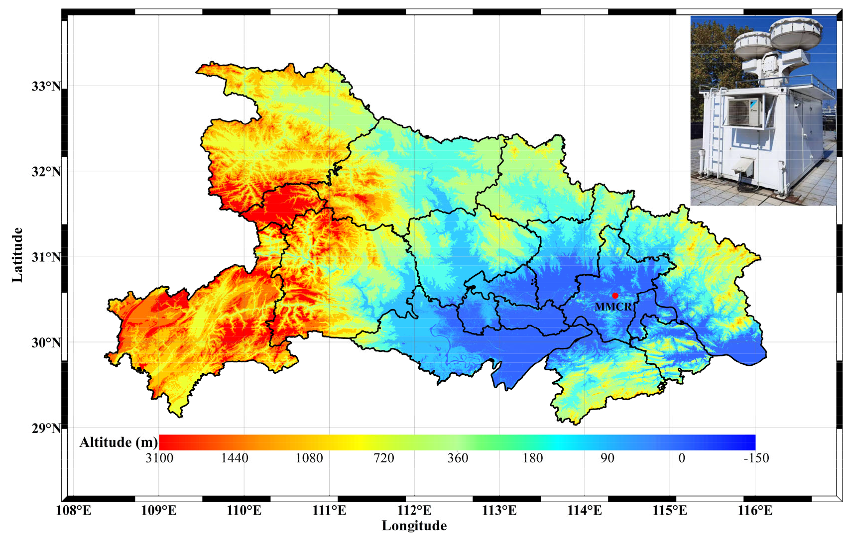
Figure 1 Topographic elevation map of Hubei Province and Ka-band MMCR located in Wuhan University (30.54° N, 114.36° E). The red spot denotes the site of MMCR.

2.1 Ka-band radar

The WHU-CW MMCR established by the ARSO adopted a continuous-wave (CW) system, and it is a Ka-band frequency-modulated continuous wave (FMCW) Doppler radar. The MMCR is installed in WHU, as shown in Fig. 1. The radar system transmits a mean power of 50 W at an operating frequency of 35.035 GHz through a 0.38° beamwidth formed by a Cassegrain antenna with 1.5 m diameter. Backscatter echoes from aerosol and cloud particles are received by the same Cassegrain antenna, and then they are sent to the signal processing subsystem to obtain the radial distribution of parameters that represent the characteristics and motion of particles, such as reflectivity factor, Doppler velocity, and Doppler spectrum width. Because of almost continuous transmitting and receiving, FMCW radar generally have a much higher mean power relative to pulse radar, which improves the capacity of MMCR to detect weak echo targets. Meanwhile, by modulating and demodulating the continuous wave, the FMCW radar measurement has an adjustable range and time resolution. In non-precipitation, the MMCR measurement has a temporal resolution of 0.26 s and a maximum measurable velocity of 4.30 m s⁻¹ without aliasing effect, which are adjusted to be 0.104 s and 10.75 m s⁻¹ in precipitation as the size and falling speed of hydrometeors increase (Mao et al., 2023), respectively. The MMCR observation has been applied to the investigations of cloud and precipitation over Wuhan in previous studies (Fang et al., 2023; Mao et al., 2023).

The MMCR has a maximum detectable distance of about 30 km and a sensitivity of −30 dBZ at the distance of 10 km. In the MMCR measurement, there are weak echoes generally less than −40 dBz within a few kilometers above the surface. The weak echoes near the surface are attributed to the backscattering of small insects and aerial plankton in some studies (Franck et al., 2021; Chandra et al., 2010; Achtemeier, 1991), and echoes are also suggested to come from the scattering of dust particles in other studies (Görsdorf et al., 2015; Clothiaux et al., 2000; Moran et al., 1998). Considering that the size of large dust particles, plant aerosol particles, and aerosol particles from combustion can be much larger than 10 µm, it is possible for the large aerosol particles to cause these weak echoes observed by MMCR. The servo-mechanical subsystem controls the MMCR to work in a specified directional mode or scanning mode. In 2020, the MMCR was operated in the vertical pointing mode, and the observations were recorded with a vertical resolution of 30 m. In this study, we attempt to explore the CBL evolution at Wuhan from the Ka-band MMCR observations in 2020.

2.2 Polarization lidar

The WHU-PL polarization lidar developed by the ARSO is also located in WHU, about 0.5 km from the Ka-band MMCR. The lidar telescope is 70 m above sea level, which is about 30 m higher than the MMCR antenna. The expanded laser beam overlaps with the full view field of the receiving telescope at a height of 0.3 km; thus, this height is the lower limit of lidar detection. The lidar data have a temporal resolution of 1 min, and the same vertical resolution of 30 m as the MMCR data. In this study, we regard the height of MMCR antenna as a baseline, and then the initial height of the lidar data is set at 0.33 km.

The lidar system consists of a transmitting subsystem, receiving subsystem, and information processing subsystem. The lidar vertically emits the laser pulses of 120 mJ at an operating wavelength of 532 nm with a repetition rate of 20 Hz by a frequency-doubled Nd:YAG laser. The output polarized laser beam has a fine polarization purity with depolarization ratio of less than 1:10 000 by using a Brewster polarizer. Light backscattered by aerosol and cloud particles as well as atmospheric molecules is collected by a telescope with 0.3 m diameter. After separated through an interference filter with 0.3 nm bandwidth centered at 532 nm, the elastically backscattered light is incident on a polarization beam-splitter prism, and then the two-channel polarized light beams are focused onto two photomultiplier tubes (PMTs). The signals from the two PMTs are transferred to a personal computer (PC)-controlled two-channel transient digitizer, which can obtain the echo signal intensity and volume depolarization ratio through the PC processing. Backscatter coefficient is retrieved based on the backward iteration algorithm under the condition of a given lidar ratio proposed by Fernald and Klett (Fernald, 1984; Klett, 1981), and then the RCS is derived from the backscatter coefficient (Freudenthaler et al., 2009; Immler and Schrems, 2003). The lidar configuration and depolarization comparison with measurements from the Cloud-Aerosol Lidar and Infrared Pathfinder Satellite Observation (CALIPSO) satellite were described in detail in an earlier study (Kong and Yi, 2015).

3 Methodology

Given that the CBLH is estimated from instruments that retrieve different variables, the algorithms that are utilized to make such estimations are also based on different principles, which are explained in the following subsections.

3.1 Gradient, variance, and wavelet transformation methods

In the lidar observation, the CBLH is derived from the RCS, which is approximately proportional to the aerosol concentration (Kong and Yi, 2015; Lewis et al., 2013; Pal et al., 2010; Emeis et al., 2008). Generally, aerosols are well mixed within the CBL due to the convectively driven turbulence, and its concentration decays sharply over the CBL top. Hence, the gradient (Grd) method is often utilized to investigate the CBLH by identifying the strongest or minimum gradient of the RCS. The wavelet covariance transformation (WCT) method, with a chosen Haar wavelet function, estimates the CBL top by investigating the correlation of the RCS variation with a step function (Zhang et al., 2021; Angelini and Gobbi, 2014; Pal et al., 2010; Baars et al., 2008; Brooks, 2003). Essentially, the WCT method can be considered a smooth enhancement of the Grd method, which may be less affected by noise than the Grd method (Davis et al., 2000; Baars et al. al., 2008).

On the other hand, because of the entrainment process, there is a frequent exchange of matter and energy between the CBL and the free atmosphere, causing the dramatic variation of aerosol concentration or lidar RCS on small timescales around the CBL top (Zhang et al., 2018; Kong and Yi, 2015). In this case, the variance (Var) method is used to determine the CBL top by identifying the maximum variance of the RCS during a relatively long period (Lammert and Bösenberg, 2006; Martucci et al., 2007; Piironen and Eloranta, 1995). We estimate the CBLH from the lidar RCS in a period of 30 min by using the three methods; for instance, the CBLH at 12:00 LT (all times in this paper are in local time) is calculated based on the RCS data from 11:45 to 12:15.

3.2 Threshold method

The variance (${\mathit{\sigma }}_{\mathrm{w}}^{\mathrm{2}}$) of vertical velocity (w) is representative of the level of turbulent activity; thus, a threshold of ${\mathit{\sigma }}_{\mathrm{w}}^{\mathrm{2}}$ was applied for determining the CBLH in the Doppler lidar measurement. The threshold is chosen to be 0.04 m² s⁻² in the regions with weak turbulence (Tucker et al., 2009), 0.3 m² s⁻² in a tropical rainforest (Pearson et al., 2010), and 0.4 m² s⁻² in the regions with a central European climate (Schween et al., 2014; Träumner et al., 2011), while thresholds of 0.1 and 0.2 m² s⁻² are selected in urban landscapes since the retrieved CBLH is not heavily dependent on the given thresholds (Burgos-Cuevas et al., 2023; Huang et al. 2017; Barlow et al., 2011). Similarly, the threshold method is also used to determine a CBLH from the more than 6000 w profiles in the MMCR measurements during a period of 30 min.

Figure 2 presents the distribution of w from the Ka-band MMCR observation and RCS (in arbitrary unit) from the lidar measurement on 15 August 2020. The day is 3 d later than the rainy day of 12 August. By taking observations for a period of 30 min from 11:45 to 12:15, we calculate the mean w and RCS, and we estimate the position of CBL top by means of different algorithms, which are shown in Fig. 3. From the lidar RCS, the CBLH is 1.35 km in the Grd and WCT methods, and it is 1.32 km in the Var method. In the MMCR observation, ${\mathit{\sigma }}_{\mathrm{w}}^{\mathrm{2}}$ has a clear downward trend with increasing height, with values of about 1.36 m² s⁻² from near the ground to 0.15 m² s⁻² at 1.47 km, and it then maintains slight fluctuations around the value of 0.15 m² s⁻² at higher altitudes. For a specified threshold of 0.3 m² s⁻², the CBL top is identified at the height of 1.35 km, which is in agreement with the lidar results.

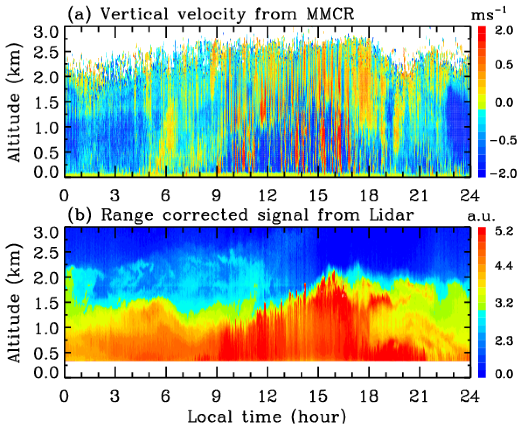
Figure 2 Time–height section of (a) vertical velocity from MMCR and (b) RCS from lidar on 15 August 2020.

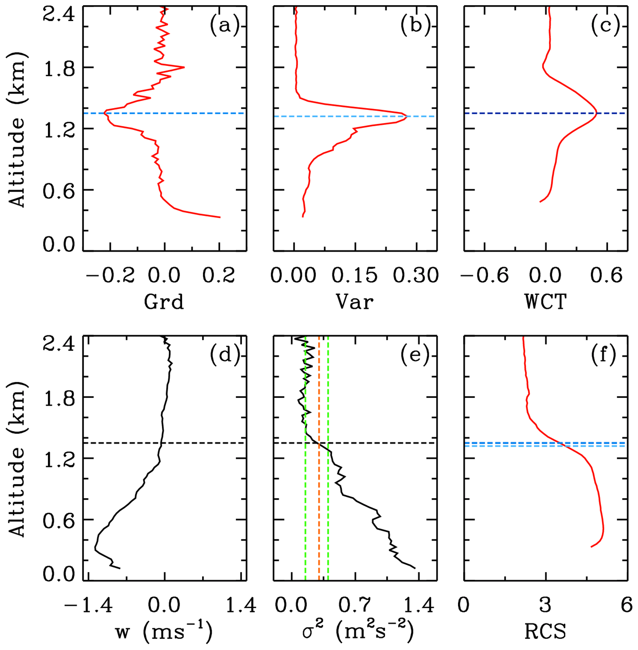
Figure 3 Profiles of (a) RCS gradient, (b) variance, (c) WCT, (f) RCS form lidar, (d) vertical velocity, and (e) its variance from MMCR between 12:15 and 12:45 on 15 August 2020. In these panels, the horizontal lines in different colors represent the CBLH determined by different methods. In Fig. 3e, the orange vertical line denotes the selected threshold of 0.3 m² s⁻², and the two green vertical lines correspond to the variances of 0.15 and 0.4 m² s⁻², respectively.

It can be noted from Fig. 3d and f that the CBLHs in the mean RCS profile are around the position with the most rapid change, while the CBLH retrieved from the MMCR ${\mathit{\sigma }}_{\mathrm{w}}^{\mathrm{2}}$ is not related to the vertical variation of mean w. So ${\mathit{\sigma }}_{\mathrm{w}}^{\mathrm{2}}$ indicates the turbulence level under the current condition, whereas RCS tends to reflect the variation in the concentration of long-time-mixing aerosol particles caused by dynamic effects (Kotthaus et al., 2023). Hence, the threshold method is a dynamical algorithm, which is more effective in capturing the dynamic changes within the CBL compared to the aerosol concentration algorithm based on the lidar RCS. In this way, the MMCR observes the high-temporal-resolution data of w, making it available for analyzing the diurnal evolution of CBL in different months and seasons. However, based on earlier studies, the selected threshold values are subject to change across the different regions (Burgos-Cuevas et al., 2023; Schween et al., 2014; Pearson et al., 2010; Tucker et al., 2009).

In Fig. 3e, ${\mathit{\sigma }}_{\mathrm{w}}^{\mathrm{2}}$ decreases quickly from 0.4 m² s⁻² at 1.29 km to 0.15 m² s⁻² at 1.47 km, indicating that the CBL top at noon is less sensitive to the selected threshold within 0.15–0.4 m² s⁻². Figure 4 depicts the CBLHs on 15 August 2020 at the thresholds from 0.2 to 0.45 m² s⁻². Nevertheless, the CBLH from 09:30 to 17:30 remains relatively stable with little change at the different thresholds, and the discrepancy among these thresholds arises mainly in the initial growing and final decaying stages of CBL.

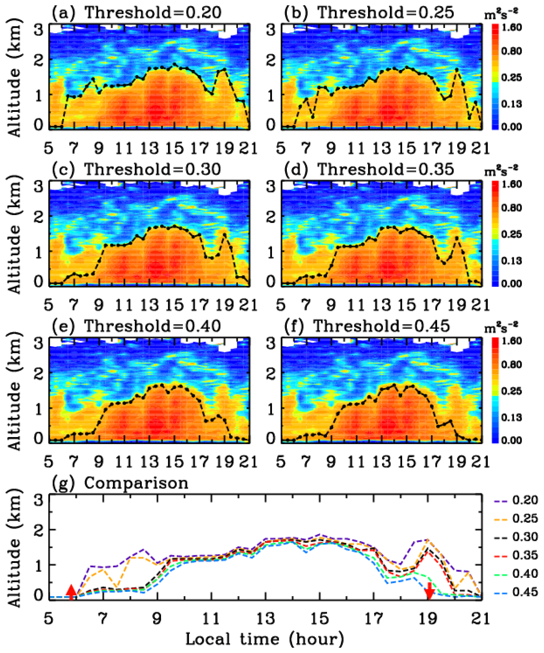
Figure 4 CBLHs derived from thresholds of (a) 0.2, (b) 0.25, (c) 0.3, (d) 0.35, (e) 0.4, and (f) 0.45 m² s⁻², superimposed over vertical velocity variance (color shading) from MMCR on 15 August 2020, and (g) their comparison. In Fig. 4g, the two red arrows denote the times of sunrise and sunset at 05:50 and 19:05, respectively.

${\mathit{\sigma }}_{\mathrm{w}}^{\mathrm{2}}$ of MMCR w determines the CBL top from the perspective of the dynamic effect, and the CBLH can be estimated from the temperature data based on the thermodynamic effect. Here, we compare the CBLH derived from the MMCR w with that from the radiosonde data. Radiosondes are typically launched in Wuhan at 08:00 and 20:00. Given that the sun has set by 20:00, we present the comparison at 08:00. The radiosonde data are provided by the University of Wyoming from the website at https://weather.uwyo.edu/upperair/bufrraob.shtml (last access: 2 May 2024). The vertical resolution of radiosonde data in Wuhan was approximately 0.5–1.0 km before June 2021, and then it was improved to a range of tens to hundreds of meters at higher altitudes. Therefore, we select the high-resolution data in the days without precipitation for our analysis.

We estimate the CBLH from the radiosonde data by using the methods of potential temperature (θ) gradient and bulk Richardson number (Ri) threshold. The potential temperature gradient (Grd_θ) is calculated at two adjacent heights in the radiosonde data, and the CBLH is determined by the maximum gradient in the profile of Grd_θ (Seidel et al., 2010). The bulk Richardson number is expressed (Zhang et al., 2014; Seibert​​​​​​​, 2000), as follows,

$$\begin{array}{}\text{(1)}& \mathit{Ri}\left(z\right)={\displaystyle \frac{(g/{\mathit{\theta }}_{\mathrm{v}s})({\mathit{\theta }}_{\mathrm{v}z}-{\mathit{\theta }}_{\mathrm{v}s})z}{(u_z-u_s{)}^{\mathrm{2}}+(v_z-v_s{)}^{\mathrm{2}}+\left(b{u}_{\ast }^{\mathrm{2}}\right)}},\end{array}$$

where g is the acceleration due to gravity; z is the height; θ_v is the virtual potential temperature; u_∗ is the surface friction velocity; u and v are the zonal and meridional wind components, respectively; and b is a constant, which is usually set to zero due to the fact that friction velocity is much weaker compared with the horizontal wind (Seidel et al., 2012). The subscripts of z and s denote the parameters at z height and surface level, respectively. In the profile of Ri, the CBLH is identified when Ri firstly crosses a threshold value upward from the ground, and the threshold is typically taken as 0.25 in earlier studies (Guo et al., 2021; Seibert, 2000), which is chosen in the analysis.

Figure 5 shows the comparisons of CBLHs derived from the MMCR and radiosonde measurements at 08:00 on 21 and 25 July 2021, respectively. On 21 July, for a threshold of ${\mathit{\sigma }}_{\mathrm{w}}^{\mathrm{2}}$ = 0.3 m² s⁻², the CBLH of 0.39 km from the MMCR w is in agreement with that of 0.40 km from the radiosonde Grd_θ, which are slightly larger than that of 0.34 km from the radiosonde Ri. In contrast to this, on 25 July, the CBLH is 0.57 km from the MMCR w, which is consistent with that of 0.59 km from the radiosonde Ri but is slightly higher than that of 0.45 km from the radiosonde Grd_θ. Nevertheless, on the whole, the results from all three methods roughly agree with each other.

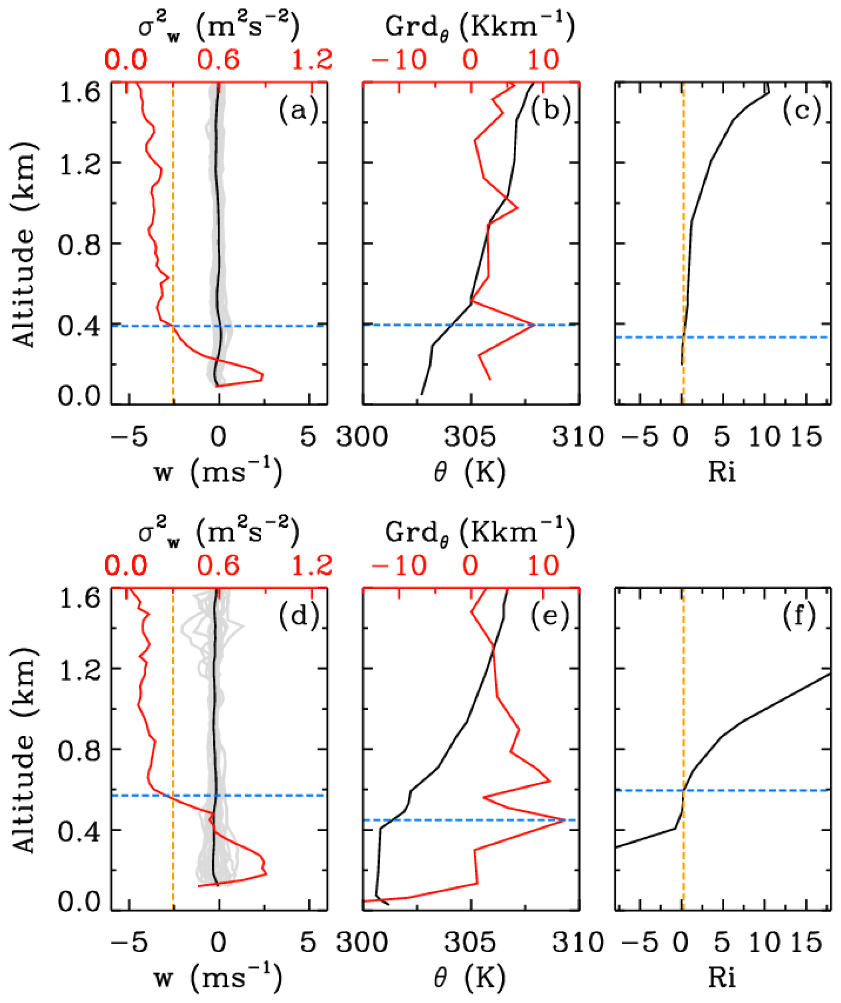
Figure 5 Comparison of CBLHs estimated by (a, d) threshold of ${\mathit{\sigma }}_{\mathrm{w}}^{\mathrm{2}}$ = 0.3 m² s⁻² from MMCR, (b, e) maximum gradient of θ, and (c, f) threshold of Ri = 0.25 from radiosonde data at 08:00 on (upper) 21 July 2021 and (lower) 25 July 2021. In panels (a) and (d), the gray and black lines denote (lower horizontal axis) w and its mean value from MMCR, respectively, and the red and yellow lines denote (upper horizontal axis) ${\mathit{\sigma }}_{\mathrm{w}}^{\mathrm{2}}$ and the threshold of ${\mathit{\sigma }}_{\mathrm{w}}^{\mathrm{2}}$ = 0.3 m² s⁻², respectively. In panels (b) and (e), the black and red lines denote (lower horizontal axis) θ and (upper horizontal axis) its gradient from radiosonde, respectively. In panels (c) and (f), the black and yellow lines denote Ri and the threshold of Ri = 0.25 from radiosonde data, respectively. The blue horizontal line represents the position of the identified CBL top.

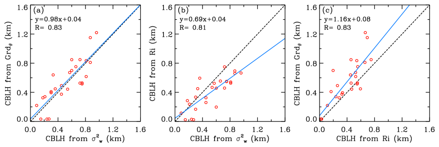
Figure 6 Scatterplot of CBLHs derived from (a) threshold of ${\mathit{\sigma }}_{\mathrm{w}}^{\mathrm{2}}$ = 0.3 m² s⁻² from MMCR vs. maximum gradient of θ from radiosonde, (b) threshold of ${\mathit{\sigma }}_{\mathrm{w}}^{\mathrm{2}}$ = 0.3 m² s⁻² from MMCR vs. threshold of Ri = 0.25 from radiosonde, and (c) threshold of Ri = 0.25 vs. maximum gradient of θ from radiosonde.

Figure 6 displays the scatterplot of CBLHs identified by the MMCR w, as well as the radiosonde Grd_θ and Ri at 08:00 on the clear days in June and July 2021. The different variables and algorithms are used in the three methods; thus, there are some differences in CBLHs derived from these methods, as shown in Fig. 6. The CBLH from ${\mathit{\sigma }}_{\mathrm{w}}^{\mathrm{2}}$ of MMCR w has correlation coefficients of 0.83 and 0.81, with that from the radiosonde Grd_θ and Ri, respectively, which are highly consistent with the correlation coefficient of 0.83 from the radiosonde Grd_θ and Ri. These results support the threshold of ${\mathit{\sigma }}_{\mathrm{w}}^{\mathrm{2}}$ = 0.3 m² s⁻² applied to the CBLH estimation in Wuhan. In the following analysis, we take 0.3 m² s⁻² as the threshold to determine the CBLH in the MMCR observation.

It can be noted that the comparison focuses solely on the CBLH at 08:00 rather than the diurnal evolution of the CBLH, owing to the lack of radiosonde observation. Consequently, we analyze the diurnal evolution of the CBLH derived from the MMCR and lidar measurements.

4 Case investigation and comparison

Figure 7 presents the CBLH evolution on 15 August 2020 from the lidar RCS based on the Grd, Var, and WCT methods, and the comparison with that obtained from the MMCR ${\mathit{\sigma }}_{\mathrm{w}}^{\mathrm{2}}$, together with the distribution of MMCR reflectivity factor in the range of 10–15 km. As shown in Fig. 7c, due to the influence of aerosol residual layer, the CBLH from the lidar RCS fluctuates from about 1.56 km at 06:00 down to 1.17 km at 09:30; however, with sunrise at 05:50, the CBL top derived from the MMCR ${\mathit{\sigma }}_{\mathrm{w}}^{\mathrm{2}}$ gradually rises from about 0.09 km at 06:00 to 1.17 km at 09:30. It is interesting that the CBLH from the lidar RCS variance drops at 07:30 and then shows a change similar to that from the MMCR ${\mathit{\sigma }}_{\mathrm{w}}^{\mathrm{2}}$. Both the variances of w and RCS represent the deviation degree of their small timescale values relative to their 30 min mean values, which may be responsible for the similar results. When the CBL ascends gradually and mixes with the residual layer, the CBLHs in the lidar and MMCR observations are consistent with each other between 09:30 and 17:00, including a slight drop at 12:30 and 14:30 (from the gradient and variance of the RCS). The maximum height of CBL is about 1.71 km at 14:00 and 15:00 based on ${\mathit{\sigma }}_{\mathrm{w}}^{\mathrm{2}}$ and the RCS gradient and variance.

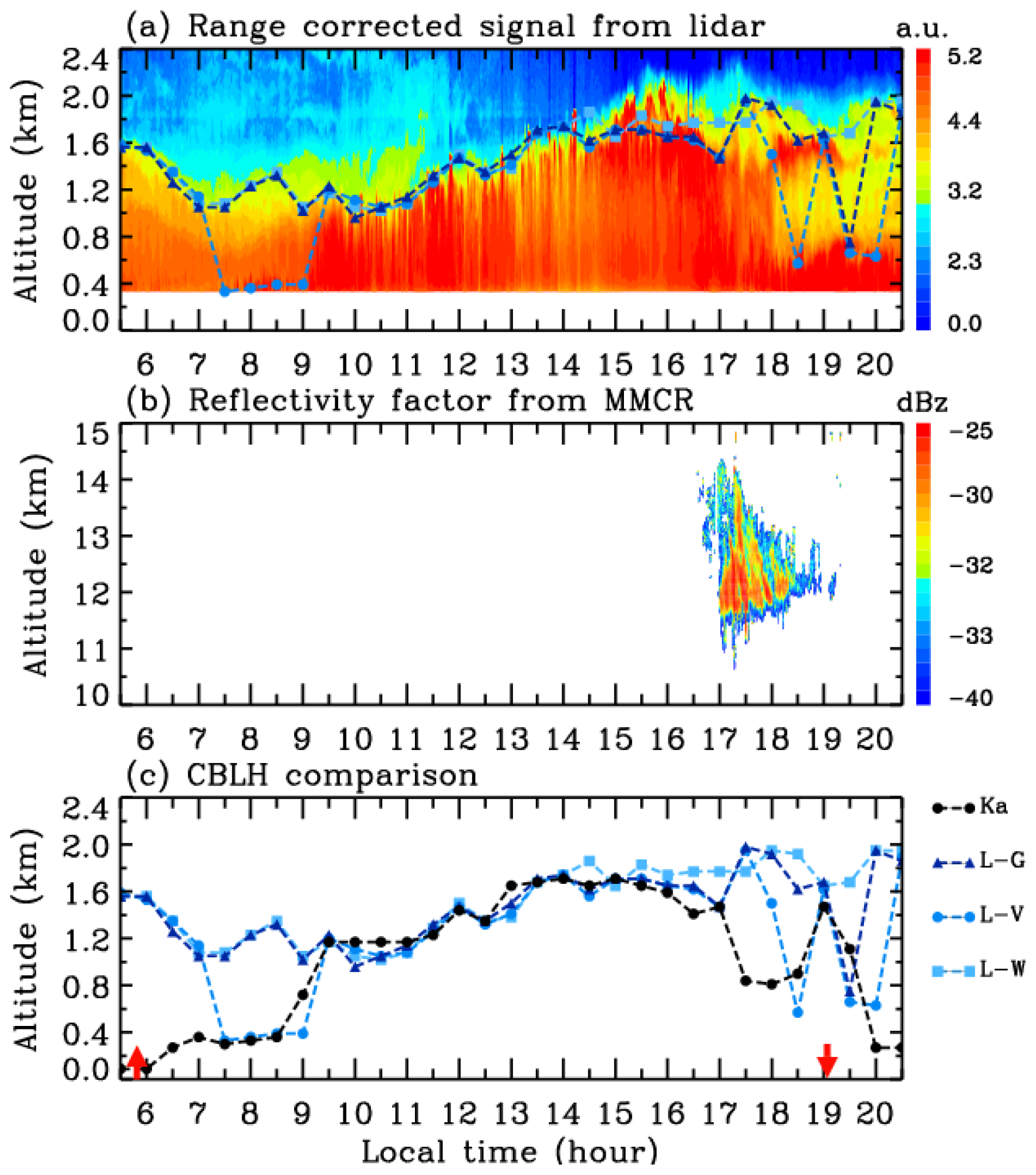
Figure 7 (a) Evolution of the CBLH derived from RCS gradient, variance, and WCT superimposed over lidar RCS (color shading) on 15 August 2020, (b) reflectivity factor from MMCR, and (c) comparison of CBLHs derived from MMCR and lidar observations. The dashed black line with circles (Ka) denotes the CBLH determined by the variance threshold of 0.3 m² s⁻² in the Ka-band MMCR observation, while the dashed dark blue, blue, and light blue lines with triangles (L-G), circles (L-V), and squares (L-W) represent the CBLH determined by the gradient, variance, and WCT methods in the lidar measurement, respectively. In Fig. 5c, the two red arrows denote the times of sunrise and sunset at 05:50 and 19:05, respectively.

One can note from the reflectivity factor distribution in Fig. 7b that cirrus clouds occur from 17:00, develop rapidly into the thick clouds at about 11–14.4 km at 17:30, and then dissipate quickly after 17:30. In the MMCR observation, the CBLH shows an obvious reduction between 17:30 and 18:30 and then a lift as the clouds dissipate rapidly. Earlier studies from the Doppler lidar w investigated the complex influence of low-level clouds on the CBL and turbulence. The cloud-top radiative cooling drives top-down convective mixing, leading to the increase in ${\mathit{\sigma }}_{\mathrm{w}}^{\mathrm{2}}$ (Hogan et al., 2009; Harvey et al., 2013; Manninen et al., 2018). During the warm season, the magnitude of ${\mathit{\sigma }}_{\mathrm{w}}^{\mathrm{2}}$ from the lidar w is large on clear-sky days and decreases on cloud-topped days, and the intensity of turbulence reduces with an increase in the cloud fraction within the CBL, except in the cloud layer that exceeds 90 % of the CBL thickness (Dewani et al., 2023). Here, the cirrus clouds are above 11 km; thus, the cloud-top-driven convective mixing has little impact on the low atmosphere; however, the thick clouds cool the surface by attenuating solar radiation, which can weaken the surface-driven convective mixing. Therefore, the thick cirrus makes a large contribution to the evident reduction of the CBLH. The phenomenon of the CBLH reduction also arises in the lidar RCS, especially from the RCS variance but with a time lag due to the influence of a long-time-mixing process on the aerosol distribution (Burgos-Cuevas et al., 2023; Schween et al., 2014). After sunset at 19:05, the CBLH retrieved by ${\mathit{\sigma }}_{\mathrm{w}}^{\mathrm{2}}$ drops quickly to 0.27 km at 20:00 from 1.47 km at 19:00, while the top of the aerosol residual layer (or horizontally migrating aerosol layer) identified by the lidar stays at a far higher level, especially from the RCS gradient and WCT.

Next, we select the observations on 31 January, 12 November, and 19 March 2020 to compare the CBLH evolution. The three dates, without clouds and precipitation, are chosen as representative of different seasons. Figure 8 shows the CBLHs on 31 January derived from the four methods above, which are overlaid on the MMCR w and ${\mathit{\sigma }}_{\mathrm{w}}^{\mathrm{2}}$ and the lidar RCS, respectively. January is the coldest month of the year, and on 31 January, the minimum (maximum) temperature is −5 °C (4 °C) recorded in the weather forecast. Owing to the convection inhibited largely by the frigid surface and air, ${\mathit{\sigma }}_{\mathrm{w}}^{\mathrm{2}}$ shows that the CBLH develops very slowly upward to 0.3 km at 11:30 from 0.12 km at 07:30 as the sun rises at 07:15. Thereafter, the top of the CBL ascends quickly to 0.9 km at 13:30, and it reaches the maximum height of 0.99 km at 14:30; during this period, the CBLH from the lidar RCS experiences a similarly rapid uplift, and it attains a peak of 1.2 km at 14:00 from the RCS gradient and variance and 1.14 km at 14:30 from the RCS WCT. In addition, it can be seen from Fig. 8d that all CBLHs from the lidar RCS are slightly larger than those from the MMCR ${\mathit{\sigma }}_{\mathrm{w}}^{\mathrm{2}}$, which may be attributed to the long-time-mixing aerosols and wet surface in winter. After 14:30, the CBLH from ${\mathit{\sigma }}_{\mathrm{w}}^{\mathrm{2}}$ descends gradually, and it approaches the ground at 17:30 prior to sunset at 17:57, while at sunset, the CBL top from the RCS is at 0.8–0.9 km due to the long-time-mixing processes.

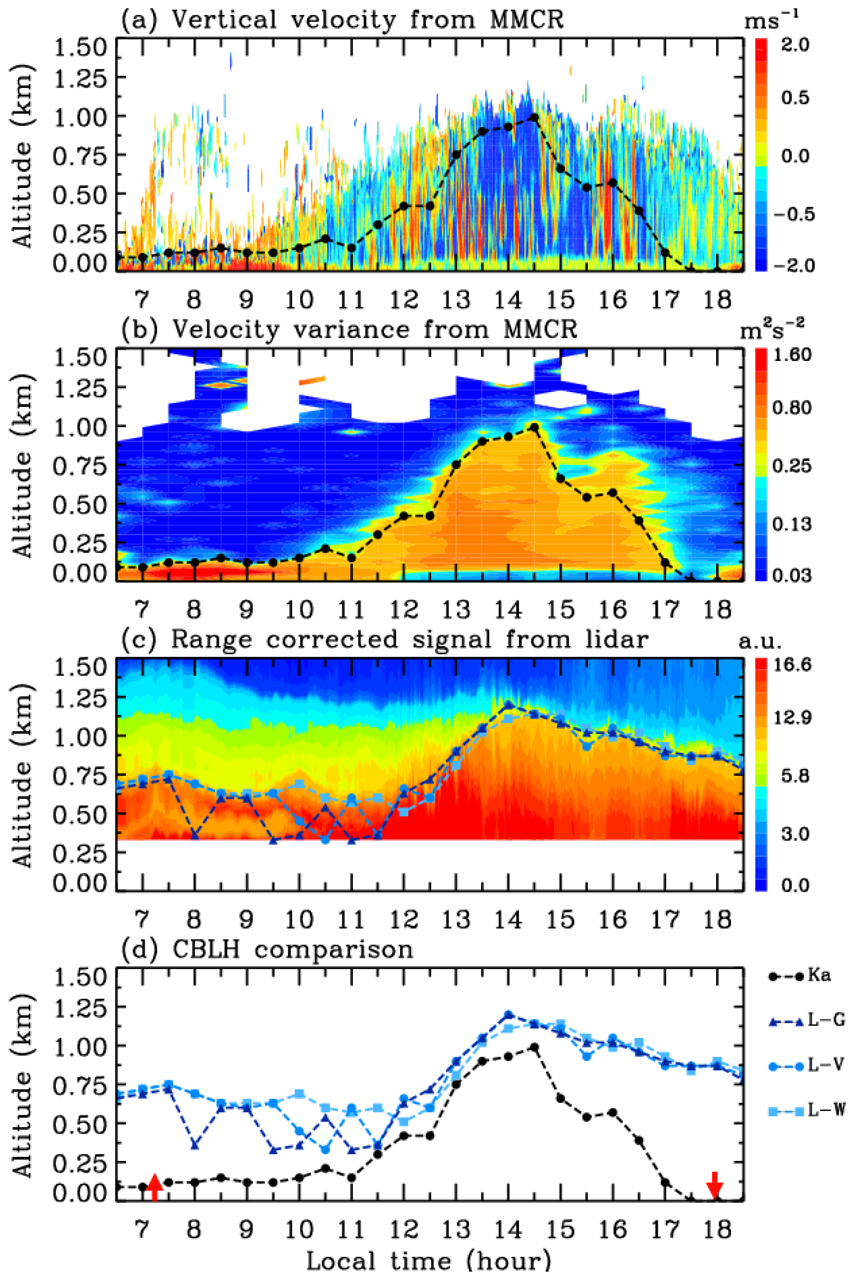
Figure 8 Distributions of (a) vertical velocity and (b) its variance from MMCR and (c) lidar RCS on 31 January 2020 with retrieved CBLH and (d) comparison of CBLHs derived from MMCR and lidar observations. The threshold of vertical velocity variance from the MMCR is 0.3 m² s⁻². In Fig. 6d, the two red arrows denote the times of sunrise and sunset at 07:15 and 17:57, respectively.

Figure 9 presents the CBLHs determined from the MMCR and lidar observations on 12 November 2020. With sunset on this day in late autumn, the CBLH identified from ${\mathit{\sigma }}_{\mathrm{w}}^{\mathrm{2}}$ displays little fluctuation until 10:30. After that, the CBL rapidly develops to 0.51 km at 11:30 and mixes fully with the residual layer retrieved from the lidar RCS; thus, the CBL tops have approximately the same evolution between the MMCR and lidar observations from 11:30 to 17:30, with the maximum values of about 0.75–0.78 km at 15:00 and 16:00. As the sun goes down at 17:27, the CBL from ${\mathit{\sigma }}_{\mathrm{w}}^{\mathrm{2}}$ rapidly shrinks close to the ground at 18:00, and aerosol particles are left in the air form a residual layer, similar to the two cases above.

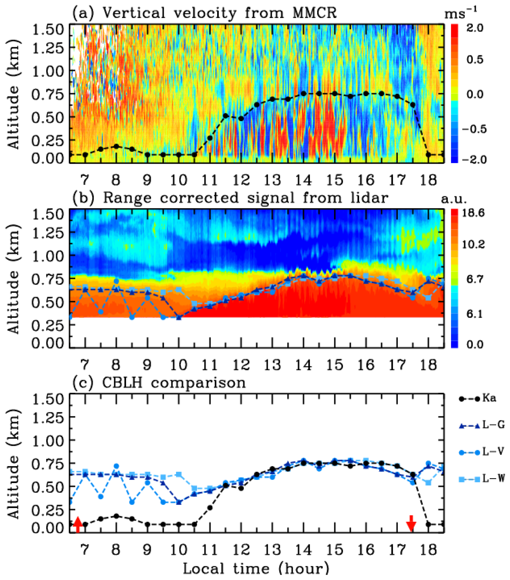
Figure 9 Distributions of (a) vertical velocity from MMCR and (b) lidar RCS on 12 November 2020 with retrieved CBLH and (c) comparison of CBLHs derived from MMCR and lidar observations. The threshold of vertical velocity variance from the MMCR is 0.3 m² s⁻². In Fig. 7c, the two red arrows denote the times of sunrise and sunset at 06:47 and 17:27, respectively.

Figure 10 depicts the CBLH variations in the MMCR and lidar observations on 19 March 2020, together with the depolarization ratio from the lidar. In spring, sand and dust with different intensities from the northwest of China frequently pass through Wuhan. On this day, there is a fine sand and dust layer mostly above 1.8 km, with the depolarization ratios of about 0.08–0.12 in Fig. 10c, which can also be noted from the distribution of w in the MMCR observation. Meanwhile, another sand and dust layer with a larger depolarization ratios of about 0.14–0.16 passes through Wuhan from about 14:00, and it mixes with the lower part of the first sand and dust layer. In this situation, the MMCR observation indicates that the CBL starts to develop gently upward from sunrise, and the upward trend of CBLH is also presented in the lidar measurement but at higher altitudes. At 09:30, the CBLH is about 0.48 km in both the MMCR and lidar observations, and then it rises steadily to 1.32 km at 16:00 and 16:30, showing a good agreement between the two observations. Subsequently, the CBLH from ${\mathit{\sigma }}_{\mathrm{w}}^{\mathrm{2}}$ undergoes two rapid declines. One occurs from 1.2 km at 17:00 to 0.51 km at 18:00, which is probably related to the sand and dust deposition in addition to the diminished radiation in the late afternoon, and the other arises after sunset. However, because of the effect of sand and dust, the CBLH from the lidar RCS increases slightly from 1.32 km at 16:30 to about 1.38 km at 18:00 and 18:30, and then it decreases gradually with time.

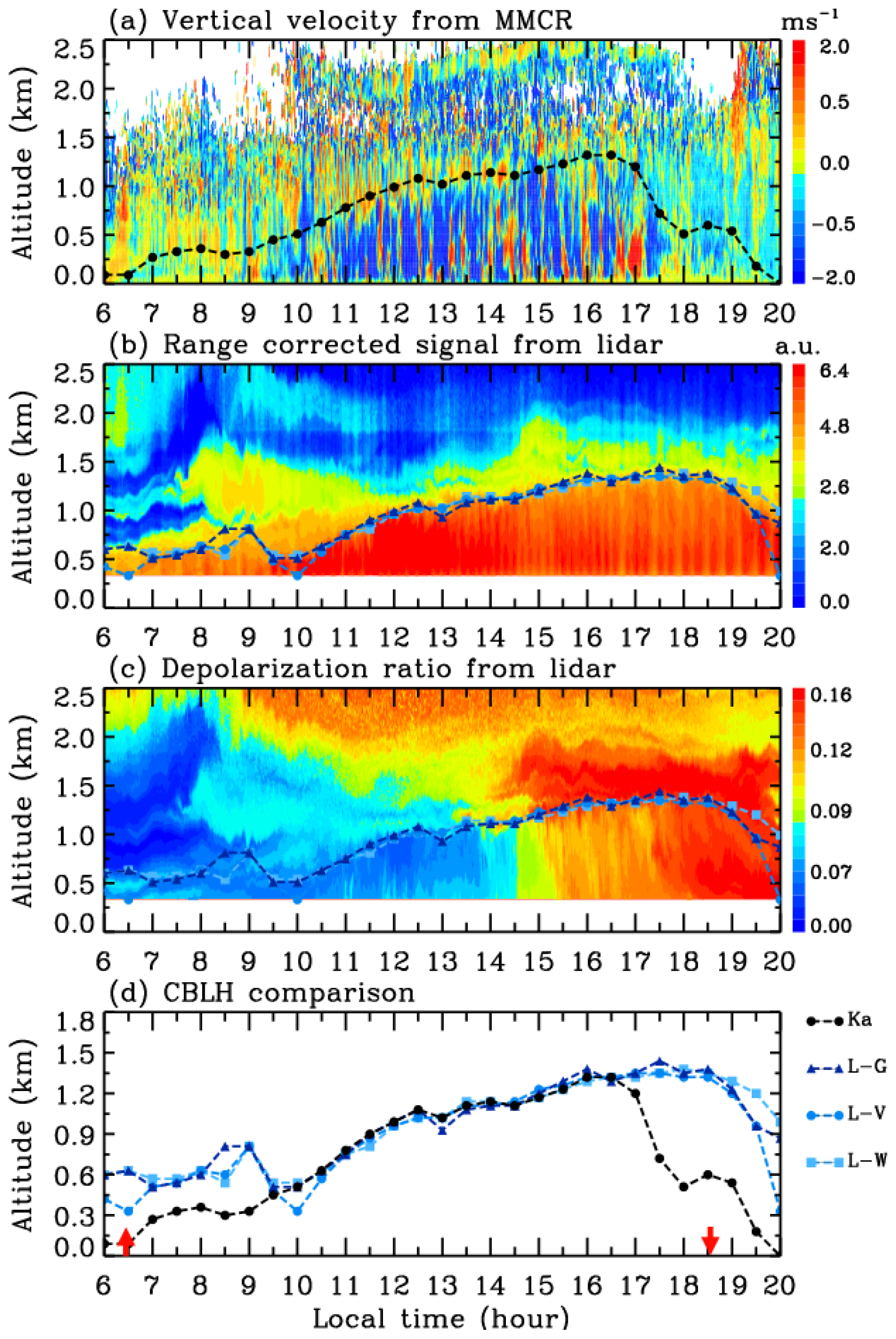
Figure 10 Distributions of (a) vertical velocity from MMCR and lidar (b) RCS and (c) depolarization ratio on 19 March 2020 with retrieved CBLH, and (d) comparison of CBLHs derived from MMCR and lidar observations. The threshold of vertical velocity variance from the MMCR is 0.3 m² s⁻². In Fig. 8d, the two red arrows denote the times of sunrise and sunset at 06:27 and 18:34, respectively.

The CBLH is identified by the spatial and temporal variations of aerosol concentration from the lidar measurement and by the temporal change in w from the MMCR observation. The four examples demonstrate that, except for the periods with the influence of aerosol residual layer, particularly during the few hours after sunrise and before sunset, the MMCR CBLHs are generally in agreement with the lidar CBLHs. The residual layer causes a higher CBLH estimated by the lidar RCS than by the MMCR w as ${\mathit{\sigma }}_{\mathrm{w}}^{\mathrm{2}}$ is less contaminated by the residual layer relative to the aerosol concentration. Additionally, the CBLH estimated by ${\mathit{\sigma }}_{\mathrm{w}}^{\mathrm{2}}$ shows a rapid response to thick high-level clouds and less influence by the long-range transport of sand and dust. Hence, the MMCR observation can accurately retrieve the CBLH and capture its diurnal evolution, especially for the CBL in the blind range of the lidar.

4.1 Monthly and seasonal mean CBLHs

To reveal the general characteristics of the CBLH diurnal evolution in different months and seasons, we calculate the monthly and seasonal mean CBLHs by using the MMCR w on these days without precipitation in 2020. We consider that winter covers the months of December, January, and February, while March, April, and May cover spring; June, July, and August cover summer; and the rest cover autumn.

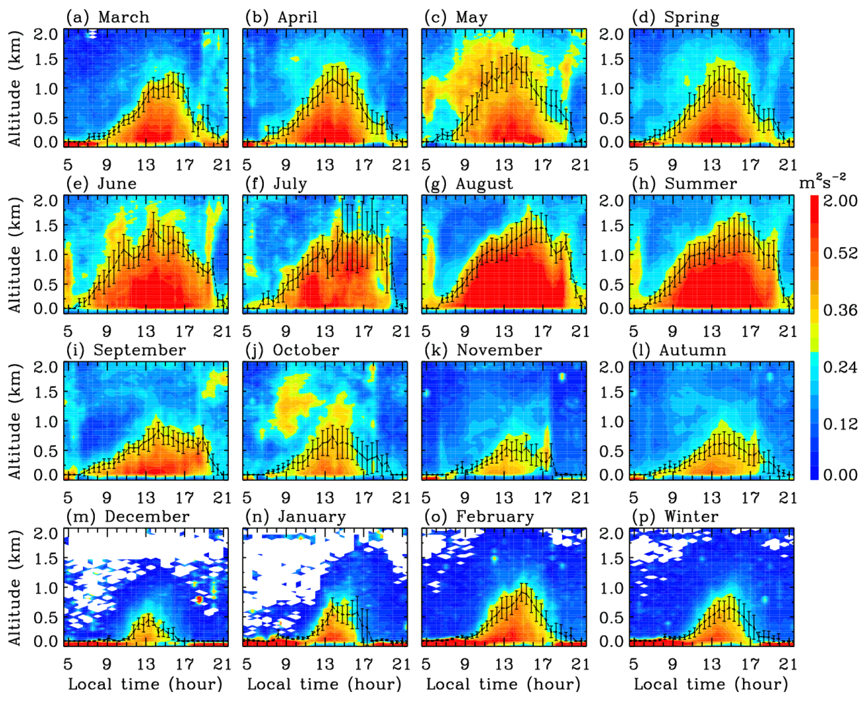
Figure 11 Monthly and seasonal mean values and statistical standard deviations of the CBLH estimated by threshold of vertical velocity variance from MMCR. The variance threshold is 0.3 m² s⁻², and the color shading denotes the variance distribution. The months and seasons are marked above the corresponding panels, respectively.

Figure 11 illustrates the averaged CBLHs with the standard deviations superimposed on the mean ${\mathit{\sigma }}_{\mathrm{w}}^{\mathrm{2}}$ in each month and season. As the spot of direct sunlight slowly moves northward, the mean variance gradually increases from January to July and then decreases gradually from August to December; moreover, the coverage height and time duration of its large values show an analogous monthly variation. In this case, the peak height of CBL ascends steadily from 0.66 km in January to 1.47 (1.44) km in July (August) and, subsequently, descends gradually to the lowest height of 0.42 km in December. Additionally, at Wuhan, the plum rain (East Asian rainy season) starts in June and prevails in July. As shown in Fig. 11, the CBLH in July has the largest standard deviation (between 13:00 and 19:00), which is possibly attributable to the cloudy and rainy weather besides the strongest radiation.

As for seasonal variation, as we expected, the mean ${\mathit{\sigma }}_{\mathrm{w}}^{\mathrm{2}}$ is the strongest in summer and the weakest in winter. Interestingly, the variance is significantly larger in spring than in autumn. Not only the maximum CBLH of 1.14 km at 13:30 in spring is much higher than that of about 0.66 km at 13:30 and 14:00 in autumn, but also the mean ${\mathit{\sigma }}_{\mathrm{w}}^{\mathrm{2}}$ of 0.42 m² s⁻² in the CBL during spring is stronger than that of 0.35 m² s⁻² during autumn. The maximum height of the CBL is 1.29 km at 14:30 and 15:00 in summer and about 0.6 km at 14:30 in winter. In summer, the CBLH displays a feature of quick descent near twilight, and in autumn, the CBL shows a wider envelope with an earlier development and a later dissipation relative to that in winter, though their maximum CBLHs are almost the same. In previous studies, based on the threshold of ${\mathit{\sigma }}_{\mathrm{w}}^{\mathrm{2}}$ from the Doppler lidar measurement in Mexico City (19.3° N, 99.1° E), the CBLH is higher in spring and summer and lower in winter, while the maximum CBLH of about 1.5 km occurs in May, which is because the CBLH is suppressed to some extent by increased cloud cover in the rainy season between June and September (Burgos-Cuevas et al., 2021). However, the CBLH retrieved from the ceilometer backscatter data is obviously larger than that from the threshold of ${\mathit{\sigma }}_{\mathrm{w}}^{\mathrm{2}}$ (Burgos-Cuevas et al., 2021; Tang et al., 2016). Similarly, in the estimation of CBLH from the lidar RCS over Wuhan and Granada (37.18° N, 3.60° E), the maximum values of seasonal mean CBLHs in all the seasons are larger than those in our results, although the gradual ascent of the CBLH from winter and autumn to spring and summer is consistent with that in our results (Kong and Yi, 2015; Granados-Muñoz et al., 2012).

5 Summary

In this study, we estimate the CBLH from the profile of w in the Ka-band MMCR observation by using a threshold of ${\mathit{\sigma }}_{\mathrm{w}}^{\mathrm{2}}$. The CBLH from MMCR is compared with that from the lidar RCS by utilizing the gradient, variance, and wavelet methods, as well as from radiosonde data by using the methods of θ gradient and Ri, which demonstrates the general agreement of the CBLH estimation based on different dynamic and thermodynamic effects. Then, we investigate the diurnal evolution of monthly and seasonal mean CBLHs based on the MMCR observation.

Although the RCS is proportional to aerosol concentration and w represents the vertical motion of aerosol particles, the comparison of the four examples in different seasons indicates that the diurnal evolution of the CBLH from the MMCR w is consistent with those from the lidar RCS, except for the initial growth and final decay phases. The discrepancy can mainly be attributed to the aerosol residual layer and the lidar blind range. The influence of residual layer on the lidar RCS generally causes an overestimation of the CBLH; meanwhile, it is impossible for lidar to capture the CBL top within its large blind range. In addition, the CBLH in the MMCR observation shows less contamination by the long-range transport of sand and dust and thick high-level clouds due to the rapid response of aerosol w relative to its concentration. In this case, the MMCR observations can capture the diurnal evolution of the CBLH.

Using the profile of w from the MMCR observation on these days without precipitation in 2020, we investigated the diurnal evolution of monthly and seasonal mean CBLHs. The maximum value of monthly mean CBLH increases gradually from 0.66 km in January to 1.47 (1.44) km in July (August), and then it decreases to the lowest height of 0.42 km in December. As for the seasonal behavior, the mean CBLH has maximum heights of 1.29 km at 14:30 and 15:00 in summer, 1.14 km at 13:30 in spring, 0.66 km at 13:30 and 14:00 in autumn, and 0.6 km at 14:30 in winter. In addition, the statistical standard deviations are dependent on month, indicating that the CBLH is not only mainly regulated by the surface heating associated with solar radiation, but also significantly affected by weather conditions, such as humidity and clouds. Therefore, since the Ka-band MMCR is a powerful instrument for observing clouds and weak precipitation, the full-time MMCR observation with low blind height can obtain the entire diurnal evolution of the CBLH, which helps us gain an insight into CBL features and also provides important input variables for weather prediction and climate models.