Estimating the variability in NO_x emissions from Wuhan with TROPOMI NO₂ data during 2018 to 2023

Accurate NO_x emission estimates are required to better understand air pollution, investigate the effectiveness of emission restrictions, and develop effective emission control strategies. This study investigates and demonstrates the ability and uncertainty of the superposition column model in combination with the TROPOspheric Monitoring Instrument (TROPOMI) tropospheric NO₂ column data to estimate city-scale NO_x emissions and chemical lifetimes and their variabilities. Using the recently improved TROPOMI tropospheric NO₂ column product (v2.4–2.6), we derive daily NO_x emissions and chemical lifetimes over the city of Wuhan for 372 d with full NO₂ coverage between May 2018 and December 2023 and validate the results with bottom-up emission inventories. We find an insignificant weekly cycle of NO_x emissions for Wuhan. We estimate a summer-to-winter emission ratio of 0.77, which may be overestimated to some extent but is still lower than suggested by the bottom-up inventories. We find a steady decline in NO_x emissions from 2019 to 2023 (except for the sudden drop in 2020 caused by the COVID-19 lockdown), indicating the success of the emission control strategy. The superposition model method results in an ∼ 15 % lower estimation of NO_x emissions when the wind direction is from distinct upwind NO₂ hotspots compared to other wind directions, indicating the need to improve the approach for cities that are not relatively isolated pollution hotspots. The method tends to underestimate NO_x emissions and lifetimes when the wind speed is > 5–7 m s⁻¹, and, in Wuhan's case, the underestimation is ∼ 4 % for the emissions and ∼ 8 % for the chemical lifetime. The results of this work nevertheless confirm the strength of the superposition column model in estimating urban NO_x emissions with reasonable accuracy.

1 Introduction

Nitrogen oxides (${\mathrm{NO}}_x\equiv {\mathrm{NO}}_{\mathrm{2}}+\mathrm{NO}$) are key atmospheric components affecting the formation of particulate matter and ozone (Bassett and Seinfeld, 1983; Jacob, 1999; Penner et al., 1991). They are emitted into the atmosphere mainly from the combustion of fossil fuels, which takes place primarily in urban areas, to heat and provide electricity to homes and businesses and to run cars and factories. Cities are responsible for more than 70 % of global NO_x emissions, and this proportion increases with the process of global urbanization and industrialization (Park et al., 2021; Stavrakou et al., 2020; Baklanov et al., 2016). Thus, accurate NO_x emission inventories for cities are required for monitoring the effectiveness of reducing air pollution and for global and regional chemical models to reproduce the complicated urban air pollution (Beirle et al., 2011). However, bottom-up city NO_x emission inventories are quite uncertain in the emission factors (Lu et al., 2015) and during the downscaling from national or regional emissions to city level (Butler et al., 2008; Lamsal et al., 2011). The top-down method using independent NO₂ observations has become widely adopted.

NO₂ has long been detected by remote sensing instruments with high quality because of its strong spectral features within the ultraviolet–visible (UV–visible) spectrum. Various satellite instruments have provided tropospheric NO₂ column measurements for near-surface NO_x emissions estimation for tens of years (Burrows et al., 1999; Bovensmann et al., 1999; Levelt et al., 2006; Veefkind et al., 2012). Limited by the coarse spatial resolution of the early instruments, researchers computed the global or regional long-term mean NO_x emissions with satellite observations and chemical transport models (CTMs) (Martin et al., 2003; Lamsal et al., 2011; Kharol et al., 2015). With the improving capabilities of later satellite sensors, more researchers started to estimate NO_x emissions on higher spatial and temporal resolutions but still depended on CTMs (e.g., Ding et al., 2017; Visser et al., 2019; Xing et al., 2022). However, there are barriers to access and employment of CTMs, and there is a substantial computational burden when the target is an individual city. Therefore, CTM-independent methods have been developed and applied to estimate NO_x emissions since the early 2010s (e.g., Beirle et al., 2011; de Foy et al., 2014; Kong et al., 2019; Beirle et al., 2019; Rey-Pommier et al., 2022).

Beirle et al. (2011) reduced the 2D NO₂ map surrounding a large point source (such as a megacity, a power plant, or a factory) to the 1D NO₂ line density by integrating the NO₂ column density across the wind direction. They developed an exponentially modified Gaussian (EMG) method to estimate NO_x emissions and lifetime from the increase in NO₂ over the source and its decay downwind of the city. Over the years, the model has been refined (Valin et al., 2013), validated (de Foy et al., 2014, 2015), applied (e.g., Lu et al., 2015; Lange et al., 2022; Goldberg et al., 2019), and extended (Liu et al., 2016, 2022). The EMG method was first applied to OMI NO₂ data to calculate NO_x emissions from cities, power plants, and factories across the globe and was shown to be accurate when wind speed is larger than 2 or 3 m s⁻¹. This method is frequently used to calculate mean NO_x emissions over longer periods (like some years) with OMI data (e.g., Lu et al., 2015; Liu et al., 2016).

At present, the much improved spatial resolution and retrieval quality of the TROPOspheric Monitoring Instrument (TROPOMI) allows the quantification of episodic (like biomass burning) or even daily NO_x emissions with the EMG method (Goldberg et al., 2019; Jin et al., 2021). Based on a single TROPOMI overpass, Lorente et al. (2019) developed a superposition column model to fit the NO₂ line density for daily NO_x emissions. They found the highest emissions on cold weekdays and the lowest on warm weekend days, indicating the significant contribution from home heating during winter in Paris. Zhang et al. (2023) used this model to estimate the daily variation in NO_x emissions over Wuhan from September 2019 to August 2020 and further inferred CO₂ emissions based on the simultaneous and co-located NO₂ and CO₂ satellite observations. The superposition column model estimates NO_x chemical lifetimes and emissions on a daily basis, avoiding the bias caused by using the averaged NO₂ columns in the nonlinear system (Valin et al., 2013). However, Lorente et al. (2019) and Zhang et al. (2023) used daily hydroxyl radical (OH) concentration from CTMs as an essential parameter, which induced computational burden when the study period is as long as several years. In addition, the CTM output OH concentration is highly uncertain (Zhang et al., 2021) and leads to uncertainty in the estimated city NO_x emissions and chemical lifetime.

In this study, we continue to focus on the city of Wuhan, extend our study period from May 2018 to December 2023, and estimate city NO_x emissions and chemical lifetimes on a daily basis with the superposition column model. We discard CTM output OH concentration in the method to reduce the results' uncertainty and improve computing efficiency. Our purpose is, firstly, to demonstrate the ability of the superposition column model to provide information on city NO_x emissions and lifetimes on interannual, seasonal, and weekly variations influenced by changes in human activity; secondly, to investigate the model performance influenced by the meteorology (wind speed and directions). The rest of the paper is organized as follows: Sect. 2 introduces the data and methods we employ in this study. In Sect. 3, we compare our results with those of other studies, analyze the temporal variability in NO_x emissions and lifetimes over Wuhan, and investigate the dependence of our estimations on the wind field. We discuss the uncertainties of this work in Sect. 4. The concluding remarks are presented in Sect. 5.

2 Data and material

2.1 TROPOMI NO₂ tropospheric columns

On 13 October 2017, the Copernicus Sentinel-5 Precursor (S-5P) satellite was successfully launched into a sun-synchronous orbit with the local overpass time at around 13:30. The TROPOMI is the only instrument on board S-5P, dedicated to air quality and climate monitoring. TROPOMI NO₂ columns are retrieved in the spectral range from 405 to 465 nm of the UV–visible spectral band with a nadir spatial resolution of 7.2 × 3.6 km² (reduced to 5.6 × 3.6 km² as of 6 August 2019) (van Geffen et al., 2020, 2022b). The small pixels and large swath width (approximately 2600 km) of TROPOMI allow the detection of localized point sources and downwind NO₂ plumes from cities on a daily basis (Beirle et al., 2019; Lorente et al., 2019).

This work uses the operational TROPOMI NO₂ version 2.4.0–2.6.0 algorithm from May 2018 to December 2023. Compared to the previous versions, v1.x, version 2.3.1 includes a different treatment of the surface albedo to avoid negative and > 1 cloud fractions, along with an updated FRESCO-wide cloud retrieval resulting in lower cloud pressures. These result in a 10 %–40 % increase in tropospheric NO₂ columns, depending on the level of pollution and season (van Geffen et al., 2022b; Lange et al., 2023). There is a major change from version 2.3.1 to 2.4.0. In v2.4.0, a new TROPOMI surface albedo climatology (directional Lambertian-equivalent reflectivity, DLER) was implemented in the cloud fraction and cloud pressure retrievals and air-mass factor calculation (Eskes and Eichmann, 2023). The use of the DLER results in a substantial increase in NO₂ columns in vegetated regions, and the higher resolution (0.125° × 0.125°) of the DLER better resolves the variability in the surface albedo (Keppens and Lambert, 2023). Version 2.4.0 performed a complete mission reprocessing from 1 May 2018 to 22 July 2022 and then switched to offline mode. Version 2.5.0 implemented a minor bug fix concerning the qa_value field over snow- or ice-covered regions. Version 2.6.0 started on 16 November 2023 and is exactly the same as version 2.5.0.

The version 2.4.0–2.6.0 Level 2 tropospheric NO₂ products are reported to be biased between +33 % (over cleaner areas) and −50 % (over highly polluted areas) compared to the ground-based MAX-DOAS data from 29 stations, with the overall negative median bias being 28 %. Amongst all the 29 ground stations, one is in Xianghe, northern China. At Xianghe, the TROPOMI tropospheric NO₂ columns correlate (R²=0.88) well with the MAX-DOAS data with a median low bias of ∼ 20 %, and the weekly averaged relative difference is within ±30 % for most of the days (Keppens and Lambert, 2023). When we use the TROPOMI data in Wuhan, some low bias is expected, and we adjust a scale factor of 1.2 to (partly) correct the bias and screen each ground pixel for the quality assurance flag (qa_value) greater than 0.75.

2.2 Wind data

Apart from the tropospheric NO₂ columns, wind field (wind direction and wind speed) is needed as a forward model parameter to determine city NO_x emissions and chemical lifetimes. We use the reanalysis wind data on pressure levels provided by the fifth-generation reanalysis (ERA5) of the European Centre for Medium-Range Weather Forecasts (ECMWF) (Hersbach et al., 2020). This dataset offers hourly wind data on 37 vertical levels with a horizontal resolution of 0.25° × 0.25°. Considering the vertical consistency of wind speeds and directions, we use the 3-level mean meridional and zonal winds below 950 hPa. The two hourly values immediately before and after the TROPOMI overpass timestamp are linearly interpolated.

2.3 Emission inventory

An initial guess of NO_x emission patterns and amounts are needed in this study, and we use the Air Benefit and Cost and Attainment Assessment System Emission Inventory (ABaCAS-EI) (Zhao et al., 2013, 2018; Zheng et al., 2019) for the year 2019 to provide this information. ABaCAS-EI is available at 1 km × 1 km gridded resolution over China, and it is developed based on activity rates and energy consumption levels with an estimated uncertainty of ±35 % (Zhao et al., 2013; Li et al., 2024b). Two other bottom-up NO_x emission inventories are also used for comparison. The first one is the Emissions Database for Global Atmospheric Research (EDGAR) v8.1, which provides monthly sectoral 0.1° × 0.1° NO_x emissions from 2000 to 2022, and the 2018–2022 data are employed. The second is the 2018–2020 monthly NO_x emission from the Multi-resolution Emission Inventory model for Climate and air pollution research (MEIC) v1.4, with a spatial resolution of 0.25° × 0.25° (Zheng et al., 2021a, b).

2.4 The superposition column model

Lorente et al. (2019) introduced this superposition column model to estimate city NO_x emissions and chemical lifetimes based on a single TROPOMI overpass and determined daily NO_x emissions over Paris. Zhang et al. (2023) modified and used this model for the Chinese city of Wuhan in a more polluted background.

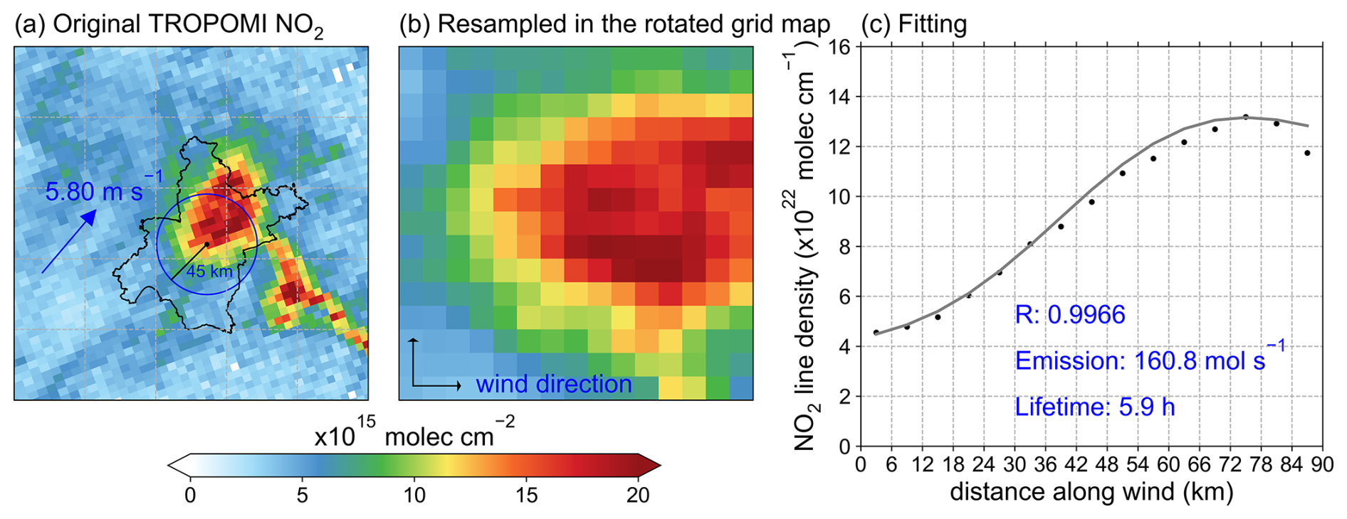
Figure 1 The analysis steps of the superposition column model. (a) The original TROPOMI NO₂ columns are on 4 March 2023. The administrative boundary of Wuhan is plotted, and the blue circle inside denotes the study domain centered on Wuhan city center (30.6° N, 114.4° E) with a 45 km radius. (b) NO₂ columns resampled on a grid map aligned with the wind direction within the study domain. (c) The grid cells perpendicular to the wind direction are integrated to obtain the NO₂ line density and fit it with the superposition column model.

Using 4 March 2023 as an example, we demonstrate the analysis steps of the superposition column model (Fig. 1). We focus on the build-up of NO₂ columns over a 45 km radius around the city center (30.6° N, 114.4° E), which covers the urban area of Wuhan (the blue circle in Fig. 1a). Compared to Zhang et al. (2023), our study domain is limited to the urban area (within the Fourth Ring Road) of Wuhan, as most (∼ 60 %) of the NO_x emissions are concentrated in the urban area (Zhang et al., 2023). In addition, since we use regional mean wind fields and NO_x chemical loss rates, the smaller study domain would reduce uncertainty in the result. We construct a 15 × 15 grid map centered at the city center with each grid size 0.05° × 0.05° (6 km × 6 km) toward the mean wind direction. One demission of the grid map is along the wind direction, and the other is perpendicular to it. The mean wind direction is determined by the mean meridional and zonal winds over the study domain. The original TROPOMI observation (Fig. 1a) is sampled into the rotated grid map (Fig. 1b). The TROPOMI NO₂ columns in the 15 grid cells perpendicular to the wind direction are integrated to form the so-called NO₂ “line densities” (Beirle et al., 2011), resulting in 15 grid cells along the wind direction (Fig. 1c).

Then, the NO₂ line density is fitted with the superposition column model (Lorente et al., 2019; Zhang et al., 2023), which is based on a simple column model (Jacob, 1999). We solve each grid cell along the wind direction with the simple column model: NO₂ builds up within the current cell and decays exponentially downwind of this cell.

$$\begin{array}{}\text{(1)}& {\displaystyle }\begin{array}{rl}{N}_i\left(x\right)& ={\displaystyle \frac{E_i}{k}}\left(\mathrm{1}-e^{-kL/u}\right)\cdot e^{-k(x-x_i)/u}\\ & \cdot {\displaystyle \frac{\mathrm{1}}{\left[{\mathrm{NO}}_x\right]/\left[{\mathrm{NO}}_{\mathrm{2}}\right]}}\text{ for }x>x_i,\end{array}\text{(2)}& {\displaystyle }{N}_i\left(x\right)=\mathrm{0}\text{ for }x\le x_i,\text{(3)}& {\displaystyle }N\left(x\right)=\sum _{i=\mathrm{1}}^n{N}_i\left(x\right)+b+\mathit{\alpha }x.\end{array}$$

NO_x emissions from cell i (E_i; mol cm⁻¹ s⁻¹) along the wind direction contribute (N_i(x); mol cm⁻¹) to the overall line density through the build-up of NO₂ within the current cell and exponential decay in the downwind cells (Eq. 1). We assume a first-order loss of NO₂ in the atmosphere. In Eq. (1), k (s⁻¹) represents the loss rate of NO₂ at the TROPOMI overpass time, and the relationship between k and NO₂ chemical lifetime ${\mathit{\tau }}_{\left[{\mathrm{NO}}_{\mathrm{2}}\right]}$ (h) is $k=\frac{\mathrm{1}}{{\mathit{\tau }}_{\left[{\mathrm{NO}}_{\mathrm{2}}\right]}\cdot \mathrm{3600}}$. Here, based on the estimation of Zhang et al. (2023), we make an initial guess as to the NO₂ chemical lifetime of 4 h for cold months (October to March) and 2 h for warm months (April to September) to derive the parameter k. We set a large range for k to allow it to change between 0.25 to 4 times the initial value. L denotes the length of each grid cell, i.e., 6 × 10⁵ cm, and u is the wind speed (cm s⁻¹). We follow Zhang et al. (2023) to take a fixed value 1.26 for $\left[{\mathrm{NO}}_x\right]/\left[{\mathrm{NO}}_{\mathrm{2}}\right]$. E_i makes no contribution to its upwind cells (Eq. 2).

The contributions from all the 15 cells are stacked up to construct the superposition column model and are combined with the contribution from the background NO₂ line densities (b+αx) to obtain the overall N(x) (Eq. 3). The initial guess of the background value b is set as the NO₂ line density at the upwind end point N(0).

The terms E_i, k, α, and b are fitted through a least-squares minimization to the TROPOMI-observed NO₂ line densities (N_TROPOMI(x)) and the a priori ABaCAS NO_x emissions (E_ABaCAS,i) to determine N(x). The cost function is defined as follows:

$$\begin{array}{}\text{(4)}& \begin{array}{rl}\mathrm{func}& ={\left({\displaystyle \frac{N\left(x\right)-N_{\mathrm{TROPOMI}}\left(x\right)}{N_{\mathrm{TROPOMI}}\left(x\right)}}\right)}^{\mathrm{2}}\\ & +\mathrm{fac}\cdot {\left({\displaystyle \frac{E_i-E_{\mathrm{ABaCAS},i}}{E_{\mathrm{ABaCAS},i}}}\right)}^{\mathrm{2}}.\end{array}\end{array}$$

The emission term is used in the cost function to reduce the dependence of fitted NO_x chemical lifetimes and emissions on the ${\mathit{\tau }}_{\left[{\mathrm{NO}}_{\mathrm{2}}\right]}$. We exert a scale factor (fac) changing between 0.1 and 0.2 to the emission term to ensure the cost function is dominated by the NO₂ line density term.

Finally, the total NO_x emissions E (in units of mol s⁻¹) from the study domain can be calculated with

$$\begin{array}{}\text{(5)}& E={\sum }_{i=\mathrm{1}}^{\mathrm{15}}{E}_i\times L,\end{array}$$

and the estimated NO_x (${\mathit{\tau }}_{\left[{\mathrm{NO}}_x\right]}$) chemical lifetime is obtained through Eq. (6) (Seinfeld and Pandis, 2016):

$$\begin{array}{}\text{(6)}& {\mathit{\tau }}_{\left[{\mathrm{NO}}_x\right]}={\displaystyle \frac{\mathrm{1}}{k\cdot \mathrm{3600}}}\cdot {\displaystyle \frac{\left[{\mathrm{NO}}_x\right]}{\left[{\mathrm{NO}}_{\mathrm{2}}\right]}}.\end{array}$$

3 Results

3.1 Mapping Wuhan's NO_x emissions and chemical lifetimes

From May 2018 until December 2023, we collect 581 overpasses with full NO₂ coverage over Wuhan. We remove the overpasses with inhomogeneous wind fields, which occur most frequently in winter. The inhomogeneous wind fields include the situations when the wind direction changes more than 45° within 2 h before the satellite overpasses, and the wind at zonal or meridional direction reverses at different pressure levels when the satellite overpasses. Multiple overpasses within 1 d are analyzed separately to calculate NO_x emissions and then averaged for the daily mean emission level.

Finally, we obtain a total of 372 d with valid NO_x emissions and chemical lifetime estimations. The number of valid days for each year and each season are summarized in Table 1. For the 5 years (2019–2023) with full-year measurement, the percentage of days with valid estimations is 15.3 %–22.5 %. Seasonally, we obtain the most valid days in autumn (defined as September to November), followed by summer (June to August). The fewest valid days occur in winter (December to February) due to the cloudy and polluted conditions.

Table 1 Number of days with valid NO_x emissions and lifetime estimations for each year and each season.

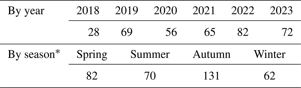
^* The days influenced by the COVID-19 lockdown (23 January to the end of April in 2020) are not considered when we count the valid days by season.

3.1.1 NO_x emissions

Zhang et al. (2023) used the superposition column model to calculate NO_x emissions over Wuhan for the period from September 2019 to August 2020. They calculated 11.5 kg s⁻¹ (equivalent to about 250 mol s⁻¹) NO_x emissions over Wuhan (including the urban area and the outskirts of Wuhan) from September to November 2019. We estimate 148.8 ± 48.8 mol s⁻¹ NO_x emissions over the urban region of Wuhan for the same period, indicating ∼ 60 % of NO_x emissions are concentrated over the central area. Lange et al. (2022) applied the EMG method to calculate NO_x emissions of 115.1 ± 10.1 mol s⁻¹ over Wuhan from March 2018 to January 2020. However, they used much earlier TROPOMI data (versions 1.1.0–1.3.0) with larger low bias and did not apply an ad hoc correction factor of 1.2 as we do in this study.

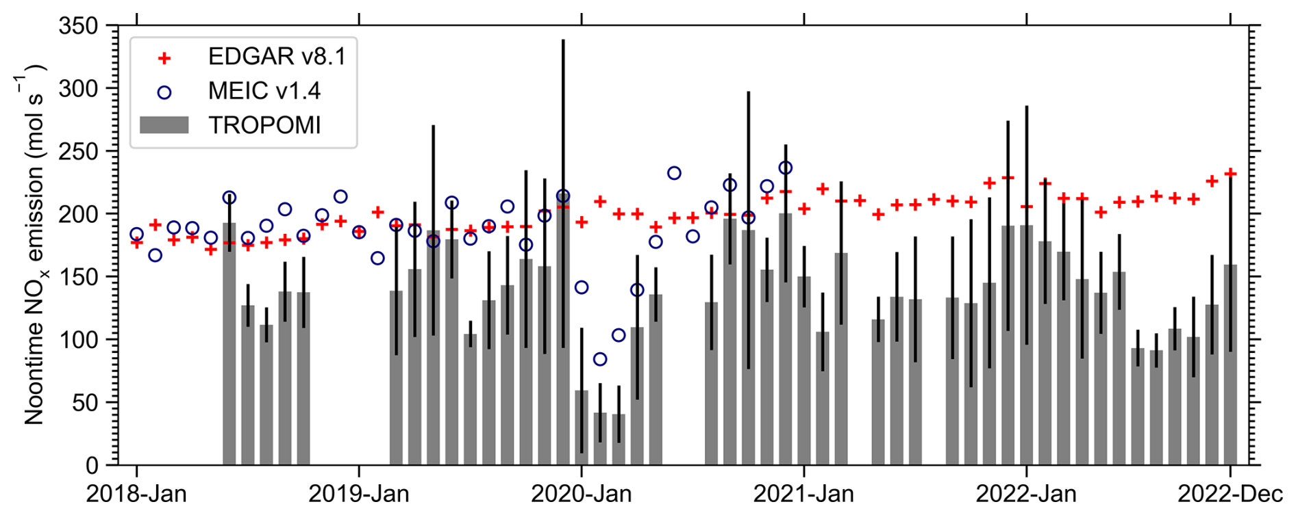
Figure 2 Monthly NO_x emissions estimated with the TROPOMI data (gray columns), reported by EDGAR v8.1 (red pluses) and MEIC v1.4 (blue circles) from 2018 to 2022 (from 2018 to 2020 for MEIC v1.4). The emissions of EDGAR v8.1 and MEIC v1.4 are scaled to the noontime emission intensities to stay consistent with TROPOMI. The TROPOMI monthly mean is calculated only when 3 or more days are available. Thus, the comparison is unavailable for several months. The error bars in the TROPOMI estimations represent the standard deviation of the daily NO_x emissions in each month.

We now compare the NO_x emissions estimated in this study over Wuhan with those from EDGAR v8.1 and MEIC v1.4 in Fig. 2. The monthly total NO_x emissions are provided in EDGAR v8.1 and MEIC v1.4, and we convert them into monthly mean noontime emission intensities with the time factor in ABaCAS-EI. Since the monthly mean TROPOMI NO_x emissions are calculated only when 3 or more days' NO_x emissions are available, the comparison is missing for the months November 2018 to February 2019, June and July 2020, April and August 2021. Overall, the TROPOMI estimation is lower than the bottom-up emission inventories, and the discrepancy is small during cold months and much larger during warm months. For the 3 years (2018 to 2020) when MEIC v1.4 data are available, the difference between TROPOMI and MEIC v1.4 is within 30 %, and both of them capture the NO_x emission reduction in early 2020 due to the COVID-19 lockdown. TROPOMI and EDGAR v8.1 are close to each other (within 20 % difference) in 2018 and 2019, but the discrepancy is larger from 2020. TROPOMI is 30 %–40 % lower than EDGAR v8.1 from 2020 to 2022.

3.1.2 NO_x chemical lifetimes

Differently to Lorente et al. (2019) and Zhang et al. (2023), we do not use the CTM-simulated daily OH concentration to constrain city NO_x chemical lifetime. Instead, we fit it around an initial value. The initial guess of the chemical lifetime for cold and warm months is determined according to the fitting results of Zhang et al. (2023).

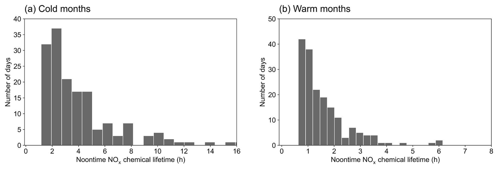
Figure 3 Distribution of estimated NO_x chemical lifetimes over Wuhan in (a) cold months and (b) warm months.

The final generated NO_x chemical lifetime over Wuhan is displayed in Fig. 3. Overall we obtain a mean NO_x chemical lifetime of 2.82 h, which is close to the 2.46 h estimated by Zhang et al. (2023) and around 5 % lower than the value (2.94 ± 0.3 h) reported by Lange et al. (2022) for the NO_x effective lifetime. For the cold months, the estimated NO_x chemical lifetime is 4.25 h, and, for ∼ 70 % of the days, the estimated NO_x chemical lifetime is between 1.5 and 6 h. For the warm months, ∼ 65 % of the chemical lifetime estimation is within the 0.8–2.5 h range, and the mean value is 1.62 h.

3.2 Temporal variability in NO_x emissions over Wuhan

Considering the atmospheric photochemical activity of NO_x, previous studies using the build-up of NO₂ pollution along the wind direction are primarily based on satellite NO₂ data in the warm months (Lu et al., 2015; Liu et al., 2016; Goldberg et al., 2021b). Lange et al. (2022) proved that it is also possible to fit the NO₂ line densities for NO_x emissions and lifetimes in winter when NO_x lifetimes are much longer. Zhang et al. (2023) estimated year-round daily NO_x emissions and lifetimes over Wuhan from September 2019 through August 2020. In this study, we extend the study period to 6 years. We have more than 40 valid days for each day of the week and more than 60 d for each season and each year (except 2018), making it possible to investigate the time variabilities in NO_x emissions over Wuhan on the weekly, seasonal, and interannual scales.

3.2.1 Weekly cycle

To identify the weekly cycle of NO_x emissions over Wuhan, we exclude the 27 valid days during the COVID lockdown period, resulting in 345 valid daily NO_x emission estimates. The weekend effect (defined as the reduction in NO₂ columns or NO_x emissions on weekends compared to weekdays) is widely recognized and reported in cities around the world but not in Chinese cities (Beirle et al., 2003; Stavrakou et al., 2020; Zhang et al., 2023; Goldberg et al., 2021a). Beirle et al. (2003) explained the absence of a weekend effect in Chinese cities by the dominant role of power plants and industry in NO_x emission sources. Stavrakou et al. (2020) found a slight reduction in NO₂ columns on weekends compared to the weekday average in Chinese cities from 2005 to 2017. Because of China's clean air action on power plants and the growing vehicle population, transportation has replaced power plants as the dominant contributor to NO_x emissions. However, we still find no significant reductions on weekends for Wuhan, as shown in Fig. 4. Wei et al. (2022) also reported weak weekday–weekend differences in surface NO₂ concentration over Chinese cities. The Annual Report on Wuhan Transportation Development (2023) (https://jtj.wuhan.gov.cn/znjt/zxdt/202409/t20240904_2450210.shtml, last access: 25 November 2024, in Chinese) revealed that the traffic flow passing through the Outer Ring Road and the Fourth Ring Road of Wuhan was highest on Fridays and lowest on Tuesdays and Sundays, but the difference is only less than 2 %. Our results also see an insignificant maximum on Fridays and minimum on Tuesdays. Cultural and living differences to other cities might explain the absence of a strong weekend effect in Wuhan. Shops, restaurants, and traffic are much busier on weekends, especially at noon when the satellite passes. Lange et al. (2022) reported a 0.79 weekday-to-weekend ratio for Wuhan; the possible reason is that our study is limited to the urban area, while a larger area is needed by Lange et al. (2022) to perform the EMG method. The different behaviors and sources in the urban and suburban areas might lead to the different weekend-to-weekday emission ratio.

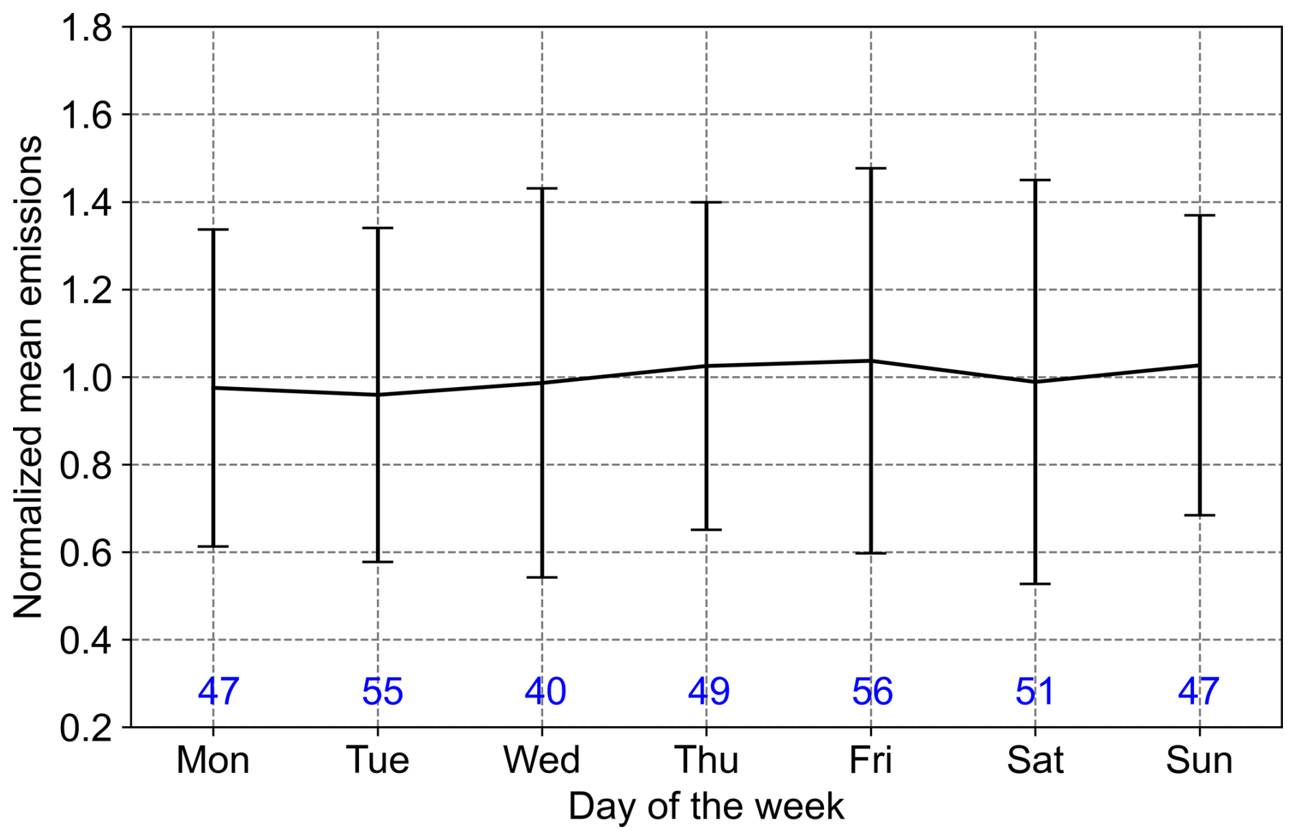
Figure 4 Weekly cycle of mean (2018–2023) NO_x emissions. The emissions are normalized with respect to the mean emissions of all the days. The number of valid measurement days for each day of the week is listed in the plot. The error bars represent the standard deviation of the daily NO_x emissions.

3.2.2 Seasonal pattern

Seasonal NO_x emissions over Wuhan are plotted in Fig. 5a. Our results reveal that Wuhan NO_x emissions vary from season to season, with the highest emissions occurring in winter and the lowest in summer. Winter emissions are higher by 9.6 %–29.4 % than the other three seasons. This is different to the bottom-up emission inventories which show little seasonal difference, as shown in Fig. 2. According to the bottom-up emission inventories, a small seasonal variation in NO_x emissions should be expected, as transportation and industry are the two dominant contributors to NO_x emissions over Wuhan, making up nearly 90 % of the total NO_x emissions, and these two emission sectors exhibit no significant seasonal variations (Zheng et al., 2018). Also, Wuhan is located in central China, where winter is mild, and there is no domestic heating in winter. The summer-to-winter NO_x emission ratio usually serves to indicate the relative importance of winter heating and summer power consumption due to air conditioning. Here we calculate a summer-to-winter ratio of 0.77, and Lange et al. (2022) reported an even lower ratio of 0.3, while it is larger than 0.85 in the bottom-up emission inventory. Two possible factors may contribute to the large difference in the summer-to-winter emission ratio between this study and Lange et al. (2022). The first is the different treatment of the NO_x-to-NO₂ ratio. We use a fixed NO_x-to-NO₂ ratio of 1.26, while Lange et al. (2022) calculated the ratio from day to day, and it was lower in summer than in winter, leading to a lower NO_x emission estimation in summer. The second factor is that we use the bottom-up emission inventory to constrain our estimation, and the flat seasonality of the bottom-up emissions leads to the higher summer-to-winter ratio of this study.

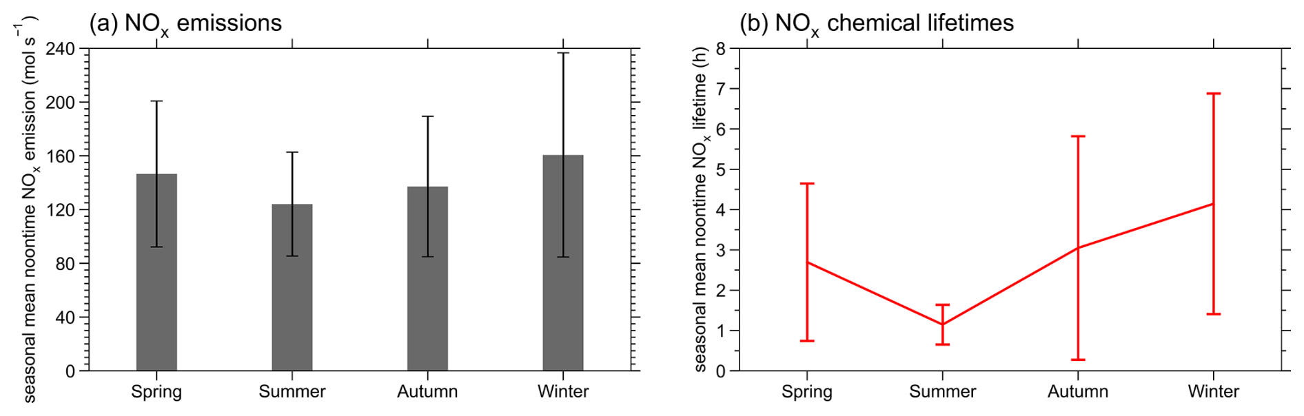
Figure 5 TROPOMI-estimated seasonal mean noontime (a) NO_x emissions and (b) chemical lifetimes over Wuhan. The error bars represent the standard deviation.

Dominated by the NO_x photochemical activity rate under the influence of temperature and OH concentrations, the NO_x chemical lifetimes are longest in winter and shortest in summer, as shown in Fig. 5b. Spring and autumn NO_x chemical lifetimes are close to each other between winter and summer. For winter, we estimate an average of 4.1 h, close to the 4.8 h reported by Zhang et al. (2023) and longer than the ∼ 3 h effective lifetime estimated by Lange et al. (2022), which makes sense, as the effective lifetime is the combination of the chemical lifetime and dispersion lifetime (Lu et al., 2015; de Foy et al., 2014). A significant difference is seen in the summer. Our estimation for summer is 1.1 h, while Lange et al. (2022) reported ∼ 2 h. With the known observed satellite NO₂ line densities, the estimated lifetime will be shorter when the estimated NO_x emissions are higher and will be shorter otherwise (Jin et al., 2021). Therefore, the reasons for the higher summer-to-winter NO_x emission ratio can also be used to explain the shorter summer NO_x lifetime in this study.

3.2.3 Interannual variation

Stringent emission control strategies have been implemented in China to control NO_x emissions to combat air pollution since as early as 2010, and a nationwide NO_x emission reduction has been seen since 2012 (Zheng et al., 2018; Li et al., 2024a). We find a similar trend over Wuhan from 2018 to 2023. Our calculation shows an increase in NO_x emissions over Wuhan from 2018 to 2019 (Fig. 6). The outbreak of COVID-19 in early 2020 led to strong changes in NO_x emissions. Studies have investigated the reduction in satellite NO₂ columns (Bauwens et al., 2020; Fioletov et al., 2022) and NO_x emissions (e.g., Ding et al., 2020; Zheng et al., 2021a; Lange et al., 2022; Zhang et al., 2021) around the world due to the lockdown restrictions to combat COVID-19. Although Wuhan reopened on 9 April 2020, we define the period influenced by the COVID-19 lockdown as 23 January to the end of April, considering the slow recovery of human activities. There are 27 d with valid NO_x emissions estimated during this period, as shown in Fig. 6. We calculated the lowest NO_x emissions of less than 20.0 mol s⁻¹ during the lockdown, and the mean NO_x emissions in this period are 49 % lower than the same period in 2019. The mean emissions during the other days in 2020 are comparable to 2019. The EDGAR data do not show a decrease in NO_x emissions during the lockdown period, while MEIC reveals an ∼ 40 % reduction (Fig. 2).

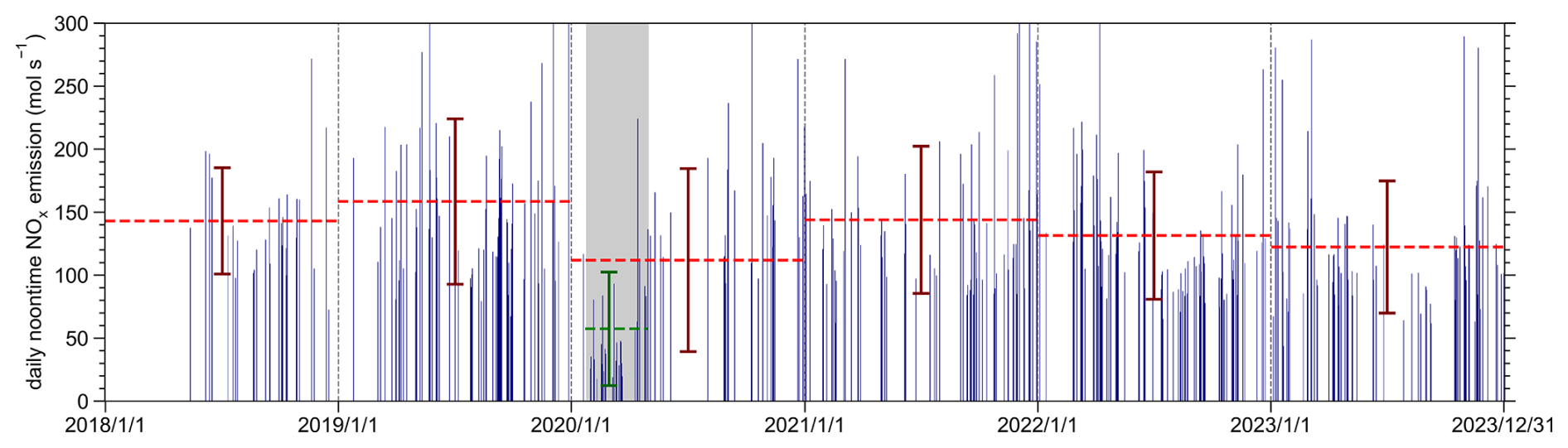
Figure 6 Daily noontime NO_x emissions over Wuhan on the days with valid estimation from 13 May 2018 through 31 December 2023. The annual mean emissions for each year are marked as dashed red lines. The dashed green line represents the mean NO_x emission during the period influenced by the COVID-19 lockdown. The error bars denote the emission standard deviation for each time frame. The period influenced by the COVID-19 lockdown is shaded in gray.

We present the estimated annual mean NO_x emissions in Fig. 6 and find a steady decrease after 2019, except the sudden drop in 2020. Considering the strong seasonality of the estimated NO_x emissions and the availability of valid days for calculation in different years, when we make the comparison between 2 years, the annual mean emissions are calculated based on the months available for both years (Lonsdale and Sun, 2023). For example, January and February estimations are absent for 2019, and June and July are not available for 2020; therefore, March to May and August to December monthly values are used to determine the annual mean emissions for the comparison of the 2 years. We find that the estimated NO_x emissions in 2020 are 10.7 % lower than in 2019, but Lonsdale and Sun (2023) reported only 5 % lower. One possible reason for the difference is that they reported a much higher estimation in October 2020. Emissions in 2021 and 2022 are close to each other and about 10 % lower than in 2019. A decrease (13.6 %) is seen in 2023 compared to 2022.

3.3 Wind field dependence of emission and lifetime estimations

Ideally, NO_x emissions and chemical loss rate directly derived from the satellite observations in combination with the wind fields should be insensitive to the wind direction and even wind speed. However, Valin et al. (2013) showed that the chemical NO_x lifetime in a city plume is wind-speed-dependent and is shorter under strong winds. The EMG method is found to provide the best emission estimations under stronger wind speed conditions (de Foy et al., 2014; Ialongo et al., 2014). This study also investigates the superposition column model performance on different wind direction and wind speed groups.

3.3.1 Wind direction

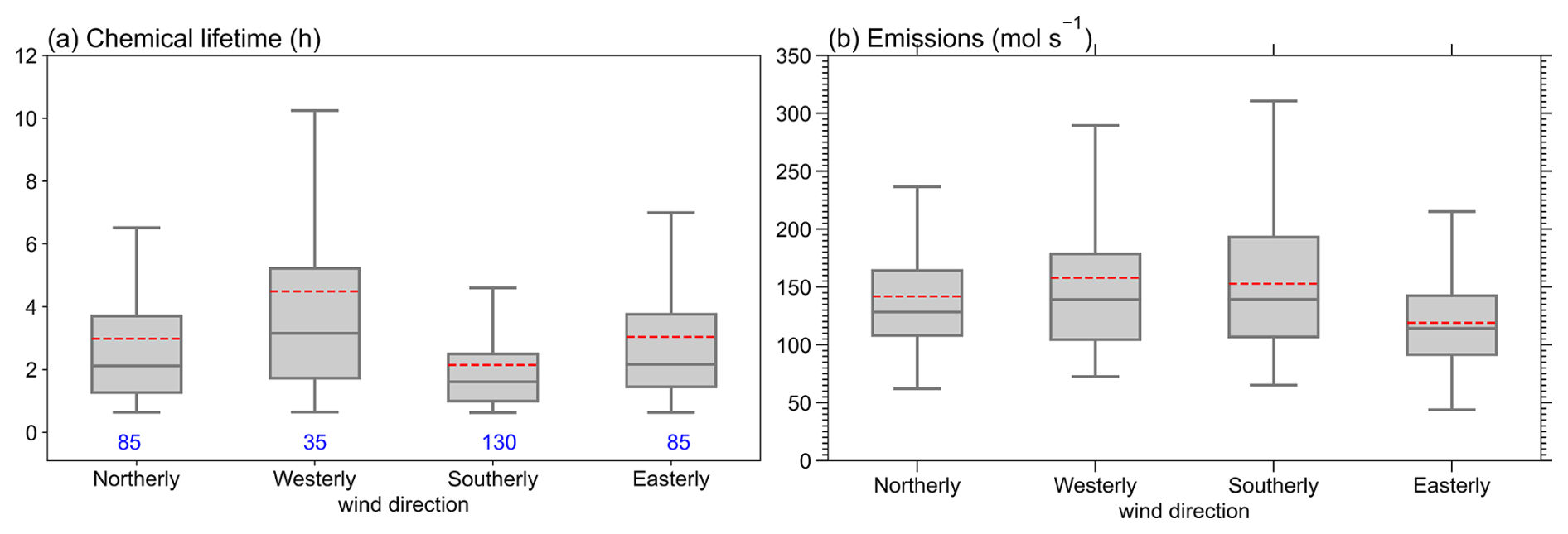
Figure 7 Boxplots of estimated NO_x (a) chemical lifetimes and (b) emissions over Wuhan are categorized into four groups based on wind direction. For each box, the middle line indicates the median; the box top and bottom indicate the upper and lower quartiles, respectively; the whiskers indicate the farthest non-outlier values; and the means are presented with dashed red lines. The number of days in each category are listed in blue.

We separate the 345 valid calculations by wind direction (northerly wind: 315–45°; westerly wind: 225–315°; southerly wind: 135–225°; and easterly wind: 45–135°) and compare the estimated NO_x lifetimes and emissions in each category in Fig. 7. The variation in NO_x chemical lifetimes with wind direction is closely related to the seasonal prevailing wind direction. About one-third of the days with westerly winds are in the winter, and more than half of the westerly wind days are in the cold months; consequently, we obtain the longest NO_x lifetimes under westerly winds. On the contrary, spring and summer are dominated by southerly winds, resulting in the shortest NO_x lifetime under this wind direction.

The estimated NO_x emissions also vary with wind direction, as shown in Fig. 7b. Emissions under westerly (southerly) winds are 12 % above (8 % below) the 345 d mean emission level, in accordance with the distribution of NO_x chemical lifetimes with the wind direction. Both the northerly and easterly winds are most abundant (∼ 50 %) in autumn, but estimated emissions under northerly winds are equal to the 345 d mean level, while it is ∼ 15 % lower under the easterly wind. When looking at tropospheric NO₂ columns over Wuhan (Fig. 1a), we find that it is relatively clean to the north, west, and south of Wuhan, but there are high NO₂ spots to the east of the city. Although we have tried to avoid the influence of upwind emissions by assuming a linear change in the background NO₂ columns (Zhang et al., 2023), the findings here indicate that it is insufficient. The high NO₂ columns at the starting point of the NO₂ line density will lead to underestimation of city NO_x emissions; the days with distinct upwind NO_x emissions should be treated cautiously in future calculations.

3.3.2 Wind speed

We then sort the 345 d with valid NO_x emission calculations into four categories according to wind speed: slow wind (0–3 m s⁻¹), medium slow wind (3–5 m s⁻¹), medium fast wind (5–7 m s⁻¹), and fast wind (> 7 m s⁻¹). We have more than 23 valid calculations for each category, and the corresponding lifetime and NO_x emissions are shown in Fig. 8.

Figure 8 Same as Fig. 7 but with the wind speed.

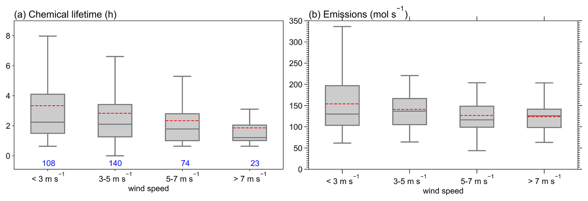
Overall, we find a decrease in NO_x chemical lifetime and emissions with the increase in wind speed, which can be explained by the fact that fast wind speed leads to strong ventilation of NO₂. Estimated NO_x chemical lifetimes decrease by 14 %–20 % as the wind speed increases (Fig. 8a). The lifetime under fast wind is nearly 40 % lower than that when the wind speed is slower than 5 m s⁻¹, in accordance with the 31 % difference calculated by Valin et al. (2013). The change in estimated NO_x emissions with wind speed is smaller (Fig. 8b). The estimated NO_x emission decreases by ∼ 20 % from < 3 to 5–7 m s⁻¹ wind speed category, and the emission changes little when wind speed is greater than 5 m s⁻¹. Thus, the superposition column model underestimates NO_x emissions and chemical lifetimes when the wind speed is faster than 5–7 m s⁻¹. The underestimation rate depends on the fraction of days with fast speed; in Wuhan's case, the overall influence is less than 4 % for emission and ∼ 8 % for chemical lifetimes.

We then look back to the varying estimated NO_x emissions in different seasons and under different wind directions. The average wind speeds in the four seasons change little, from 3.8 to 4.8 m s⁻¹, falling into the 3–5 m s⁻¹ wind speed group. This indicates that the lower summer-to-winter NO_x emission ratio estimated by the top-down method (this study and Lange et al., 2022) than the bottom-up emission inventories cannot be attributed to the decreasing estimation with wind speed. In addition, the average wind speeds in the four directions vary from 3.5 to 4.5 m s⁻¹, eliminating the influence of the decreasing estimation with wind speed on the lower estimated emissions under easterly winds.

4 Discussion on the uncertainty

We use the superposition column model to estimate city NO_x emissions and chemical lifetimes on a daily basis, and the results are used to analyze the temporal variability in NO_x emissions over Wuhan. There are factors leading to uncertainties in our estimation and analysis.

The uncertainties of NO_x emission and lifetime estimations come from the parameters and quantities used during the fitting procedure. The primary sources of uncertainties include the following:

• The systematic error in TROPOMI NO₂ data. The TROPOMI version 2.4.0–2.6.0 data showed significant improvements from the earlier versions, and there is an ∼ 20 % difference compared to the ground-based data at the Xianghe site in northern China (Keppens and Lambert, 2023); we have corrected the possible underestimation over Wuhan by a factor of 1.2, but we still conservatively consider a 20 % uncertainty in the NO₂ column.

• Upwind emissions. We find a 15 % anomaly in estimated NO_x emissions and an 8 % anomaly in NO_x chemical lifetime for Wuhan when there are distinct hotspots of NO₂ in the upwind region. We thus take the uncertainty of 15 % (for emissions) and 8 % (for chemical lifetime) to represent the influence of upwind emissions. We must clarify that this part of the uncertainty is “city-specific”. It can be neglected for some isolated cities or large point sources like Paris or Riyadh. For other cities located in polluted backgrounds, the uncertainty induced by upwind emissions should be calculated accordingly, and it should not necessarily be 15 % or 8 %.

• Bottom-up NO_x emissions. We use bottom-up emissions to constrain our estimations. Uncertainty in the bottom-up emission inventory is 35 % (Zhao et al., 2013; Li et al., 2024b), and we found that it has a 10 % influence on the estimated NO_x emissions and a 30 % influence on the chemical lifetime estimation.

• The ${\mathit{NO}}_x/{\mathit{NO}}_{\mathrm{2}}$ ratio. Uncertainty arising from the ${\mathrm{NO}}_x/{\mathrm{NO}}_{\mathrm{2}}$ ratio is 10 %, in accordance with that from Zhang et al. (2023).

• Wind fields. Uncertainty caused by the wind fields partly comes from the systematic wind error, which we take as 20 % following Zhang et al. (2023); the other part comes from the limitation of the superposition column model, and we exert 4 % for emission and 8 % for chemical lifetime estimation. This part of uncertainty is also “city-specific”, and the uncertainty increases as the mean wind speed increases in the study domain.

Finally, we use the root-mean-square sum of all the above contributions, resulting in a 35 % uncertainty for the NO_x emissions and 44 % for NO_x chemical lifetimes estimated for Wuhan. It is noteworthy that Zhang et al. (2023) considered the uncertainty caused by the area of the study domain and the CTM-simulated OH concentration, and they found a 15 % and 20 % uncertainty caused by the two factors separately. In this study, we leave out the consideration of the uncertainty caused by the size of the study domain because our study domain is limited to the urban area of Wuhan, and it is a proper size to estimate NO_x emissions in the urban area. We discard the model-simulated OH concentration in the fitting procedure so that the uncertainty caused by the OH concentration is avoided. We give an initial guess on the NO_x chemical lifetimes, the uncertainty of which is not considered because we let it vary in a quite large range; the initial value would have little influence on the fitting.

Uncertainties also exist in the analysis of the temporal variability in the estimated NO_x chemical lifetimes and emissions. First, our conclusion about the insignificant weekly effect of NO_x emission over Wuhan might be reliable, since this is also found in the surface NO₂ and O₃ concentration (Wei et al., 2022; Yang et al., 2020), indicating no significant weekday/weekend difference in the oxidation environment. We may have overestimated the summer-to-winter emission ratio (0.77), although this ratio is even higher in the bottom-up emission inventory. As we stated in Sect. 3.2.2, the fixed ${\mathrm{NO}}_x/{\mathrm{NO}}_{\mathrm{2}}$ ratio and the fact that the bottom-up emissions are used to constrain the NO_x emissions will lead to a lower estimated summer-to-winter emission ratio. In addition, even though v2.3.1 and later have higher retrieval in winter and over polluted areas (van Geffen et al., 2022b), they are still found to be lower in polluted areas and higher in clean areas when compared to the ground measurements (Keppens and Lambert, 2023). As a consequence, we may still underestimate winter emissions and/or even overestimate summer emissions, thus leading to a higher estimated summer-to-winter emission ratio. Thirdly, when comparing 2 years' emissions, the annual mean emissions are calculated based on the months available for both years instead of the average of all valid days. In this way, we have minimized the uncertainty caused by the different availability of valid days in different years. However, the reliability of our results needs more years of estimation and more bottom-up information to confirm.

5 Conclusions

In this work, we use the superposition column model to calculate city NO_x emissions and chemical lifetimes on a daily basis, with a time span of nearly 6 years, from May 2018 to December 2023. The city of Wuhan is used as an example to investigate the seasonal pattern, weekly cycle, and interannual variation in city NO_x emissions. The dependence of the model performance on the wind direction and speed are also discussed. We choose the urban area of Wuhan as our study domain, which has a 45 km radius around the city center. For each day with full NO₂ coverage with a homogeneous wind field, the TROPOMI NO₂ columns are sampled in a 15×15 grid that is aligned with the wind direction. Then, every 15 grid cells perpendicular to the wind direction are accumulated to form the NO₂ line density. The NO₂ line density is fitted with the superposition column model to obtain the final daily NO_x emissions and lifetimes.

For the period from May 2018 to December 2023, we obtain 372 d with valid NO_x emission and lifetime estimations over Wuhan, with more than 60 d for each season and each year (except 2018) and more than 40 d for each day of the week. The monthly NO_x emissions from 2018 to 2022 are compared with those from EDGAR v8.1 and MEIC v1.4 (until 2020) bottom-up emission inventories. TROPOMI estimation is lower than MEIC by less than 30 % for 2018–2020. Compared with EDGAR v8.1, TROPOMI estimation is lower by ∼ 20 % for 2018 and 2019 but 30 %–40 % lower in 2020–2022. We find a 0.77 summer-to-winter NO_x emission ratio, which might be biased high, though it is even higher in the bottom-up inventory (> 0.85). The estimated noontime NO_x lifetimes vary from 1.1 h in summer to 4.1 h in winter, with an average of 2.8 h. We see an insignificant weekly cycle for Wuhan, which may be related to the living culture and style of the Chinese. We find that NO_x emissions over Wuhan during the period influenced by the COVID-19 lockdown are nearly 50 % lower than the normal level and rebound to the 2019 emission level for the rest of 2020. Overall, our calculations reveal a steady decline in NO_x emissions from 2019 to 2023.

Compared to previous studies using the superposition column model (Lorente et al., 2019; Zhang et al., 2023), we discard the CTM-simulated OH concentration in the derivation of NO_x chemical loss rate. By doing so, we make this method CTM-independent and computationally efficient, and we also avoid the uncertainty caused by the OH concentration. We use the bottom-up emission inventory to constrain the emission estimation, which induces about 10 % uncertainty and leads to overestimation of the summer-to-winter emission ratio.

We separate the 345 d (excluding 27 d during the COVID-19 lockdown) of NO_x emissions and lifetimes according to wind direction and speed to investigate the model performance under the influence of the wind field. We find ∼ 15 % lower estimated NO_x emissions in conditions with distinct upwind emissions, indicating that we need to be more careful in the future when computing NO_x emissions over cities or large point sources located in a polluted background. Because of the ventilation of NO₂ under fast wind speed, the estimated NO_x chemical lifetime and emissions decrease as the wind speed increases. Thereby, the estimation will be underestimated for the sources dominated by fast winds.

We have demonstrated in this work that, by combining the superposition column model and the high-spatial-resolution TROPOMI NO₂ column product, one can investigate the variability in NO_x emissions and lifetimes on daily to annual timescales. We also provide recommendations for dealing with conditions with upwind emissions and high wind speeds for better and more accurate city NO_x emission estimations. So far, the superposition column model has only been used for two cities, Paris and Wuhan; we will extend it to other cities and emission sources in the future.