Measurement report: An investigation of the spatiotemporal variability in aerosols in the mountainous terrain of the upper Colorado River basin using SAIL-Net

In the western US and similar topographic regions across the world, precipitation in the mountains is crucial to local and downstream freshwater supplies. Atmospheric aerosols can impact clouds and precipitation by acting as cloud condensation nuclei (CCN) and ice-nucleating particles (INPs). Previous studies suggest that there is increased aerosol variability in these regions due to their complex terrain, but none of these studies have quantified the extent of this variability. In the fall of 2021, Handix Scientific contributed to the Surface Atmosphere Integrated Field Laboratory (SAIL), funded by the US Department of Energy (DOE) and situated in the East River watershed (ERW; Colorado, USA), by deploying SAIL-Net, a novel network of six aerosol measurement nodes spanning the horizontal and vertical domains of SAIL. The ERW is a topographically diverse region, meaning individual measurement sites can miss important observations of aerosol–cloud interactions. Each measurement node included a small particle counter (the Portable Optical Particle Spectrometer – POPS), a miniature CCN counter (CloudPuck), and a filter sampler (the Time-Resolved Aerosol Particle Sampler – TRAPS) for INP analysis. SAIL-Net studied the spatiotemporal variability in aerosols and the usefulness of dense measurement networks in complex terrain. After the project's completion in the summer of 2023, we analyzed the data to explore these topics. We found increased variability compared to a similar study over flat land. This variability was correlated with the elevation of the sites, and the extent of the variability changed seasonally. These data and analyses serve as a valuable resource for continued research into the role of aerosols in the hydrologic cycle and as the foundation for designing measurement networks in complex terrain.

1 Introduction

In mountainous regions, winter snowpack and overall precipitation are vital for maintaining local and downstream freshwater supplies. In these areas, atmospheric aerosols play a role in local precipitation patterns by acting as cloud condensation nuclei (CCN) and ice-nucleating particles (INPs) (Jirak and Cotton, 2006; Lynn et al., 2007). It is therefore critical to understand and monitor aerosol concentrations in these areas. Ambient aerosols are spatially and temporally complex due to their many sources and relatively short atmospheric lifetimes (Anderson et al., 2003; Weigum et al., 2016). This complexity is further amplified in mountainous terrain (Zieger et al., 2012; Yuan et al., 2020; Nakata et al., 2021). Direct measurements of aerosols across spatial and temporal scales are therefore essential to fully understand the role of aerosols in cloud formation and precipitation.

Orographic clouds, formed by topographically forced upward motion, are an important contributor to winter snow in mountainous regions. In these clouds, ice crystals form in the upper layers and then fall through a supercooled liquid layer, collecting rime and growing larger before reaching the ground as snow or graupel. This process is sensitive to the number of CCN and INPs present (Creamean et al., 2013; Levin et al., 2019). The amount of rime gathered by descending crystals is contingent upon the size of the supercooled liquid droplets, with smaller droplets being less efficiently collected. In CCN-rich clouds, the droplets are smaller, resulting in reduced rime and overall precipitation. In the Rocky Mountains of Colorado, Saleeby et al. (2011) found that decreased riming causes a shift in precipitation from windward to leeward slopes and potentially into different watersheds. The riming process is also inversely influenced by INPs, where higher concentrations of INPs increase precipitation (Rosenfeld et al., 2014). Thus, understanding the spatial and temporal variability in atmospheric aerosols is necessary to understand the role of aerosols in the hydrologic cycle in mountainous regions and subsequent impacts on freshwater availability.

To further study land–atmosphere interactions and their impact on the hydrologic cycle in mountainous regions, the US Department of Energy (DOE) supported the Surface Atmosphere Integrated Field Laboratory (SAIL), located in the East River watershed (ERW) of the upper Colorado River basin in southwestern Colorado. The Colorado River basin covers parts of Colorado, Utah, Nevada, New Mexico, and California, as well as all of Arizona. These states withdraw an average of 20 billion m³ of water each year (Maupin et al., 2018). In the past 20 years, this basin has experienced increasingly intense droughts, leading to concern over freshwater availability in the western United States. Precipitation is affected by anthropogenic aerosols, and it is estimated that the Colorado River basin loses approximately 66 million m³ of water each year due to an increase in CCN caused by anthropogenic emissions (Jha et al., 2021). Thus, one of the main goals of the SAIL campaign was to improve Earth system modeling to better predict the timing and availability of water resources from the mountains in this region.

Two monitoring sites were deployed in the East River watershed from the fall of 2021 to the spring of 2023 as part of the SAIL campaign. These two sites were the aerosol observation system (AOS) located at Crested Butte Mountain Resort and the second Atmospheric Radiation Measurement (ARM) mobile facility (AMF2), located at the Rocky Mountain Biological Laboratory in Gothic, Colorado. Both sites collected a variety of aerosol and atmospheric measurements (Feldman et al., 2023). While these two sites provided comprehensive aerosol measurements, they may not have fully represented the complete spatial variability in aerosol concentrations due to the complex terrain of the region (Schutgens et al., 2017). Thus, additional measurement locations were beneficial, if not crucial, to understanding aerosol–cloud interactions in this complex terrain.

To gain a more comprehensive understanding of aerosols in the region, we deployed SAIL-Net, a distributed network of six measurement nodes spanning the domain of the SAIL research area, from October 2021 to July 2023. Each node measured aerosol particles between 140 nm and 3.4 µm in diameter using a small particle counter (the Portable Optical Particle Spectrometer – POPS; Gao et al., 2016), CCN using a miniature CCN counter (CloudPuck), and INPs using the Time-Resolved Aerosol Particle Sampler (TRAPS; Creamean et al., 2018). Our approach was similar to that of other studies that aimed to better characterize and understand aerosols and gas-phase pollutants using networks of lower-cost sensors (Caubel et al., 2019; Kelly et al., 2021; Asher et al., 2022). Such studies have identified neighborhood-level variations in pollutant concentrations (Schneider et al., 2017; Popoola et al., 2018; Caubel et al., 2019). Small-scale variations such as these are poorly represented in models and poorly measured by a single monitoring system (Caubel et al., 2019). Previous work has shown that the representation error (the ability of measurements to represent larger areas) increases with complex orography, leading to decreases in model accuracy (Schutgens et al., 2017). The overall goal of SAIL-Net was to improve our understanding of the variability in aerosols in the ERW, thus increasing our knowledge of aerosol–cloud interactions in this region and assessing the usefulness of distributed networks of measurements for future studies. We met this goal by answering the following scientific questions:

1. What is the aerosol temporal variability, and how does aerosol inhomogeneity vary seasonally? Is there significant seasonal variability in the sources, or are short-term meteorological conditions the most important determining factor for sources of cloud nuclei?

2. What is the aerosol spatial variability? What are the aerosol characteristics at the cloud base? Are these particles, as presumed, the most representative of those acting as cloud nuclei?

3. How should measurement networks be designed to capture aerosol–cloud interactions, and what do they need to measure? Can a single measurement site accurately represent aerosol properties in regions with complex terrain?

The goal of this paper is to introduce SAIL-Net, highlight initial observations from the POPS data, and use these findings to address the scientific questions. We hope these data and analyses inspire future research on the variability and impact of aerosols in mountainous terrain.

Section 2 of this paper introduces the instrumentation, sites, and data pertaining to SAIL-Net. Next, Sect. 3 uses the data from the POPS instruments to address our scientific questions and highlights the trends observed in the data. This section is divided into three subsections. First, Sect. 3.1 identifies the temporal variability in aerosols in the ERW by looking at seasonal and diurnal patterns. Next, Sect. 3.2 highlights the spatial variability in aerosols in the region and suggests conditions and sources that may affect this variability. Lastly, in Sect. 3.3, we compare the network as a whole to determine whether a single measurement site could sufficiently represent the ERW.

2 Methods

Each site included a suite of three relatively low-cost, lightweight microphysics instruments manufactured by Handix Scientific to measure aerosol size distributions (POPS), CCN concentrations (CloudPuck), and INP concentrations (TRAPS). Together, this network of instruments provided a comprehensive picture of aerosol–cloud interactions in the region. These instruments were chosen and used in combination because their size, price, low power requirements, and self-sufficiency made them the optimal choice for supporting a distributed network of sites in remote terrain.

The three instruments were secured inside a weatherproof enclosure and mounted on 3 m tall scaffolding to keep them above the snow in the winter. The inlets of the instruments faced downward and were protected by a baffle. Four of the six sites ran on solar power, while the other two sites used established ground power sources.

This paper focuses on data from the Portable Optical Particle Spectrometer (POPS). The POPS is a small, low-cost optical particle counter initially developed at NOAA by Gao et al. (2016) and later commercialized by Handix Scientific. In the last few years, it has been recognized for its accuracy and reliability as a low-cost sensor and has been used in a number of field deployments and campaigns (Mei et al., 2020; Brus et al., 2021; Asher et al., 2022; Todt et al., 2023). This instrument measures the intensity of light scattered by particles passing through a 405 nm laser to optically size particles into bins of different sizes (selected by the user), ranging from approximately 140 nm to 3.4 µm, and does so at a 1 s resolution.

The POPS instruments operated continuously at each SAIL-Net node, except during power outages, deep snowfalls that temporarily buried some inlets, or other instrument malfunctions. This is the largest and longest dataset produced by SAIL-Net.

2.1 Network description

SAIL-Net consisted of six measurement nodes spread across the ERW, located near Crested Butte, Colorado. The primary objective in selecting site locations was to capture the vertical variation in aerosol properties while also covering the full domain of the SAIL campaign. The elevation of the sites ranged from roughly 2750 m along the valley floor of the ERW to approximately 3500 m near the top of Crested Butte, which is one of the taller peaks in the ERW. The farthest distance between the sites was 14 km, while the closest two sites were approximately 1 km apart. The disparate elevations of the sites resulted in different types of vegetation surrounding each site. Table 1 describes each site. A map of the sites is provided in Fig. 1, and Fig. 2 provides photos of each site.

Table 1 Locations and brief descriptions of the six SAIL-Net sites in the East River watershed.

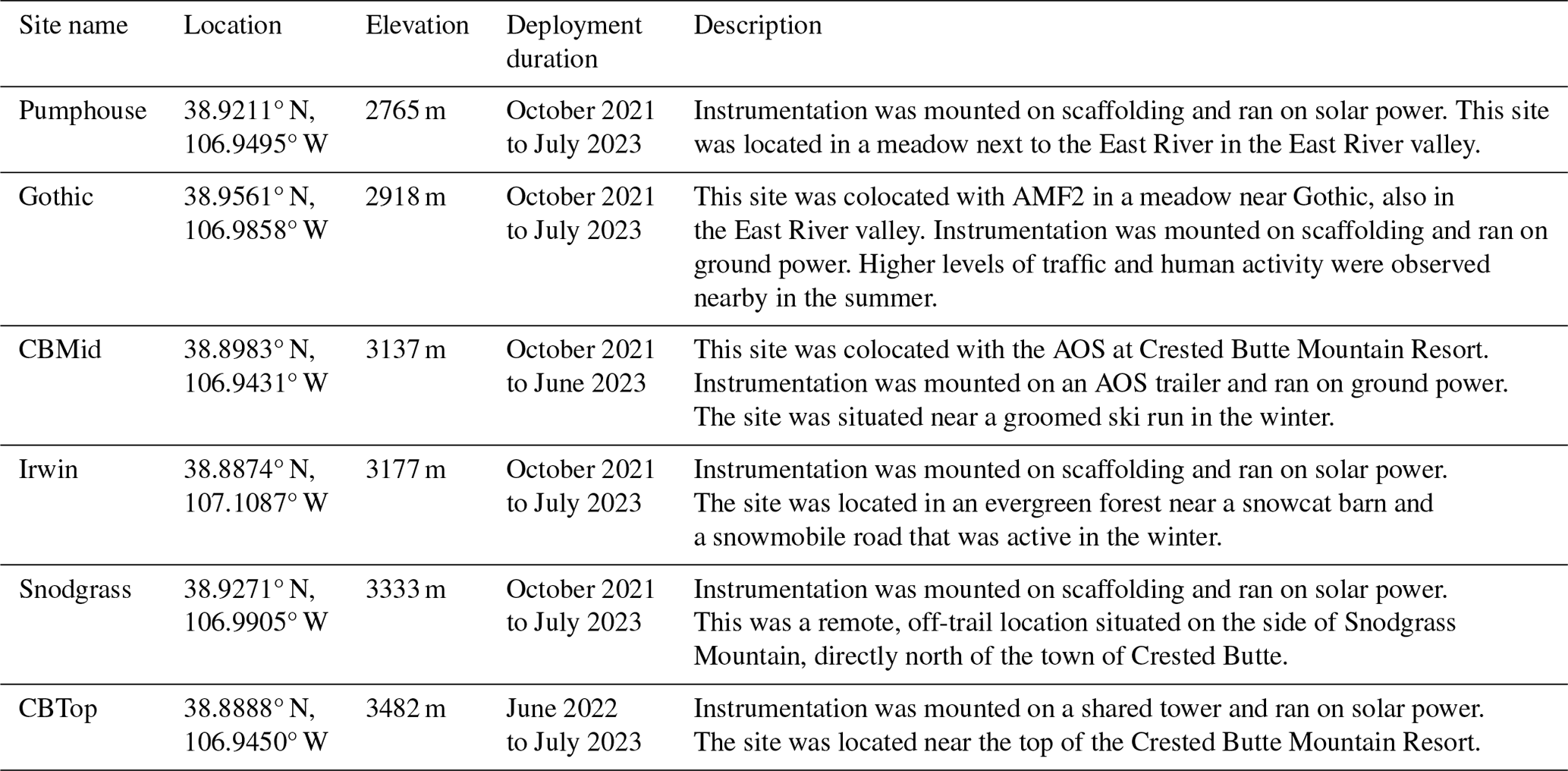
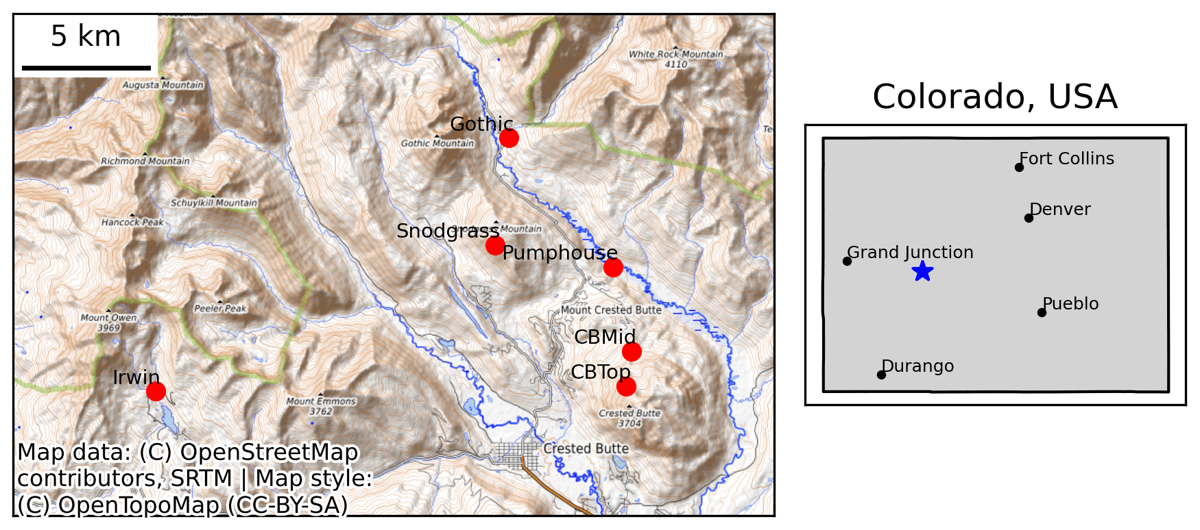
Figure 1 The panel on the right shows a map of the state of Colorado, USA. The region where SAIL-Net measurements were taken is marked with a blue star. The panel on the left shows a zoomed-in topographic map of this region, with the six SAIL-Net sites marked with red dots. The network spanned a vertical distance of approximately 8 km (north–south) and a horizontal distance of 14 km (east–west) and covered approximately 750 m of elevation difference. © OpenStreetMap contributors 2024. Distributed under the Open Data Commons Open Database License (ODbL) v1.0. SRTM: Shuttle Radar Topography Mission.

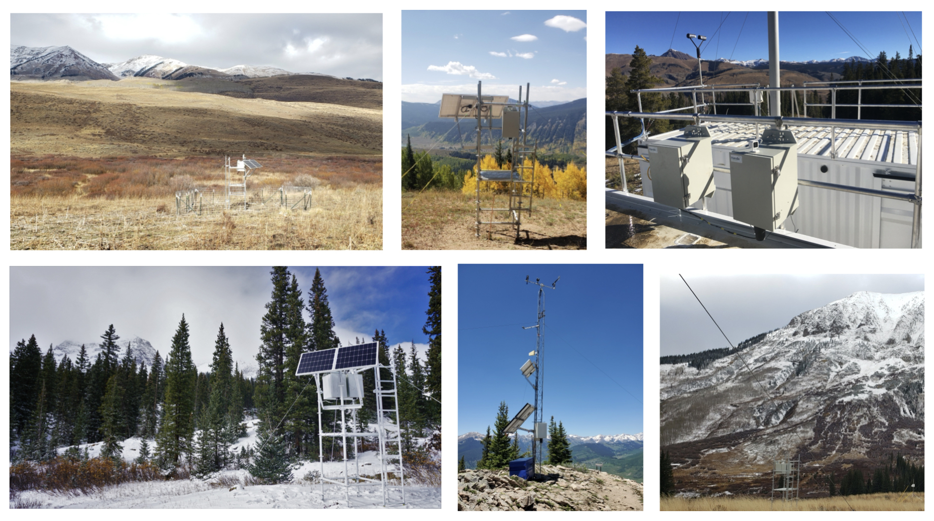
Figure 2 Photos of the six sites in SAIL-Net. On the top row (from left to right), the sites are Pumphouse, Snodgrass, and CBMid; on the bottom row (from left to right), the sites are Irwin, CBTop, and Gothic. Four of the sites ran on solar power, and the solar panels can be seen in the photos. CBMid and Gothic both ran on ground power.

2.2 Data acquisition and post-correction

The SAIL-Net sites were visited approximately monthly. During each visit, a suite of checks were performed to ensure instrument reliability and to document instrument drift. The POPS instruments underwent the most checks and monitoring. We checked the inlet flow of the instrument and recorded the accuracy of each POPS in sizing 495 nm aerosolized polystyrene latex (PSL) beads (PSL check). This information was later used to post-correct the data. Figure S1 in the Supplement shows an example of how these PSL checks appear in the raw data. We did not recalibrate the POPS instruments in the field to correct for drift at any point during the campaign to avoid causing discontinuities in the raw data. However, if any of the instruments required major repairs, they were removed, repaired, or replaced, with instruments returned the following month as needed. When a new or repaired POPS was deployed in the field, its sizing was recalibrated. In these cases, there was some discontinuity in the sizing accuracy, but this was corrected in the post-analysis data, as discussed below.

The data collected by each POPS in SAIL-Net were binned into one of 16 bins as number counts based on the measured size of the particles. These number counts were converted to number concentrations in publicly available datasets (Gibson and Levin, 2023). In diameter space, the widths of the bins are not equal but increase non-monotonically with size. The size range of the particles for smaller bins is approximately 15 nm, while the size range for larger bins is approximately 600 nm. The following description provides insight into why the bins have unequal widths in diameter space and why this increase is not strictly monotonic.

The data correction process focused on correcting drift in the POPS sizing accuracy. All POPS instruments in SAIL-Net experienced some drift, but the drift rate and amount were not uniform across the different instruments. We collected data from the PSL checks during the majority of the site visits (but not all). Some sites were not visited during certain months due to accessibility issues, or the PSL check was not performed due to instrument malfunctions or weather conditions. Thus, some assumptions were made during post-correction to account for these gaps. We assumed that the POPS instruments were performing at their factory calibration level at the start of the measurement period – the fall of 2021 (or the summer of 2022 in the case of CBTop, the site located near the top of the Crested Butte Mountain Resort) – and therefore did not need post-correction until drift was observed during the PSL check. We also assumed that the PSL checks were representative of an entire month. Lastly, if a PSL check was missed in a given month, we assumed that the drift was linear to allow for interpolation between the missing PSL checks.

The post-correction process involved shifting the boundaries of the bins to place the PSL beads in the correct bin once the data correction process was complete. A POPS experiences drift for two primary reasons: either the laser diode loses intensity over time, or the mirror that reflects light becomes dirty. In either case, the lower intensity of light causes particles to be measured as smaller than their true size, meaning the drift of each POPS monotonically decreases over time. The bin that contains the 495 nm sized particles has a lower bound of 350 nm. Thus, drift is recognized when the PSL beads are measured as smaller than 350 nm, shifting the bin in which the PSL signal occurs.

As a particle passes through the beam of the laser diode, the light is scattered, and the digitizer in the POPS reads the raw signal of the light intensity. The sizing range of each POPS is determined by taking the base-10 logarithm of the range of the digitizer. In logarithmic space, the range extends from 1.75 to 4.806. The bins of the POPS instruments are then determined by dividing this range into n bins of equal width (w), where

$$\begin{array}{}\text{(1)}& w=(\mathrm{4.806}-\mathrm{1.75})/n.\end{array}$$

These logarithmic values are converted to diameter space using Mie theory. In diameter space, the bins are no longer equal in width.

The reasoning behind the post-correction comes from considering the raw signals that the digitizer receives and scaling the signal to properly bin it. The following explanation shows that this is equivalent to simply shifting the current bins of the POPS instruments. When the POPS sizes particles accurately, the 495 nm PSL beads should be placed into the bin containing 495 nm sized particles. Let the midpoint of this bin in logarithmic space be called x. Suppose the PSL beads are instead distributed into a different bin with a midpoint (y) in logarithmic space. In this case, the digitizer would observe a raw signal of 10^y instead of 10^x. To correct for this error, we would need to scale all raw signals by ${\mathrm{10}}^x/{\mathrm{10}}^y$. Since this is a post-correction process and all raw signals have already been received, we instead scale all digitizer bin boundaries by ${\mathrm{10}}^x/{\mathrm{10}}^y$ so that the drifted signals are binned properly. The bin boundaries, collectively denoted by b_i, are defined in logarithmic space using the range of the digitizer and Eq. (1), but they can be converted to a raw signal using ${\mathrm{10}}^{b_i}$. Thus, to account for the drift, we apply a shift to all bin boundaries, expressed as ${\mathrm{10}}^{b_i}({\mathrm{10}}^x/{\mathrm{10}}^y)$. To then convert the raw signal back to logarithmic space, which is necessary for converting it back to diameter space, we apply the base-10 logarithm of the raw boundaries as follows:

$$\begin{array}{}\text{(2)}& {\log }_{\mathrm{10}}\left({\mathrm{10}}^{b_i}\right({\mathrm{10}}^x/{\mathrm{10}}^y\left)\right)=b_i+(x-y).\end{array}$$

Since x and y are the midpoints of equally sized bins in logarithmic space, (x−y) is equivalent to the width of a bin (w) multiplied by the number of bins between these midpoints (m). Thus, the post-correction process ends up being as simple as shifting all bins by m spaces (keeping the bin boundaries the same) until the 495 nm PSL beads, as well as all particles, are sized correctly.

As an example, if the PSL check placed 495 nm particles into a bin one size smaller, the post-correction process would move all particles from the first bin into the second, all particles from the second bin into the third, and so on. Then, the particles that were previously sized as 143 to 155 nm in the first bin would now be sized as 155 to 170 nm, adopting the size range of the second bin. Because of this upward shifting, the smallest size that the POPS instruments measured increased throughout the deployment. For the majority of the following analysis, the minimum particle size used will be 170 nm (the minimum of the third POPS bin), instead of the 140 nm size that is standard with the POPS, to account for this shift. This shift allows for a fair comparison across sites, even with a drifted POPS. If a POPS shifted by more than two bins, its data were not used in the following analysis. Pumphouse experienced the most drift, where, in the last month of the deployment, particles were distributed into bins four sizes smaller. Snodgrass experienced the least drift, with the PSL check still sizing particles properly at the end of the deployment. Table S1 in the Supplement contains a table showing the monthly documented drift for each POPS.

Once data were rebinned, additional smoothing was performed by computing 1 min rolling averages of the data to remove excessive noise. These post-corrected and cleaned data were used for all analyses described in the following section. All time series plots and analyses use Coordinated Universal Time (UTC) timestamps unless otherwise noted. Figure 3 displays the coverage of the particle size data, ranging from 170 nm to 3.4 µm, for each site in the network. We assume that the post-correction process removed any instrument-caused variation between the different POPS instruments and, therefore, that the remaining variability observed in the data is due to environmental conditions. These cleaned POPS data, raw POPS data, and CloudPuck data are all publicly available via the ARM Data Discovery portal (Gibson and Levin, 2023). The INP data will become available once the filters have been analyzed by Perkins et al. (2023).

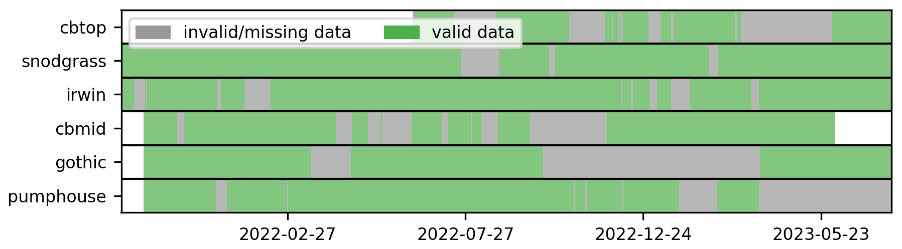
Figure 3 Coverage of the 170 nm–3.4 µm POPS data for each day. The days marked as having “invalid/missing data” indicate days when the site was in place but either no data were recorded or the data did not meet quality assurance standards. The days marked as having “valid data” indicate days when the site had valid data. The white spaces indicate periods when the site was not yet or no longer in place. The percentages of valid data for the sites are as follows: 60 % for CBTop, 92 % for Snodgrass, 88 % for Irwin, 76 % for CBMid, 66 % for Gothic, and 75 % for Pumphouse.

3 Results and discussion

This section uses data from the six POPS instruments to address the scientific questions proposed in the Introduction. The POPS instruments produced the longest dataset with the highest temporal resolution, allowing for the study of spatiotemporal variability in aerosol concentrations and distributions. Figure 4 displays the complete time series of concentration data for 170 nm–3.4 µm sized aerosol particles from the POPS instruments at the six sites. The data were averaged daily with respect to UTC.

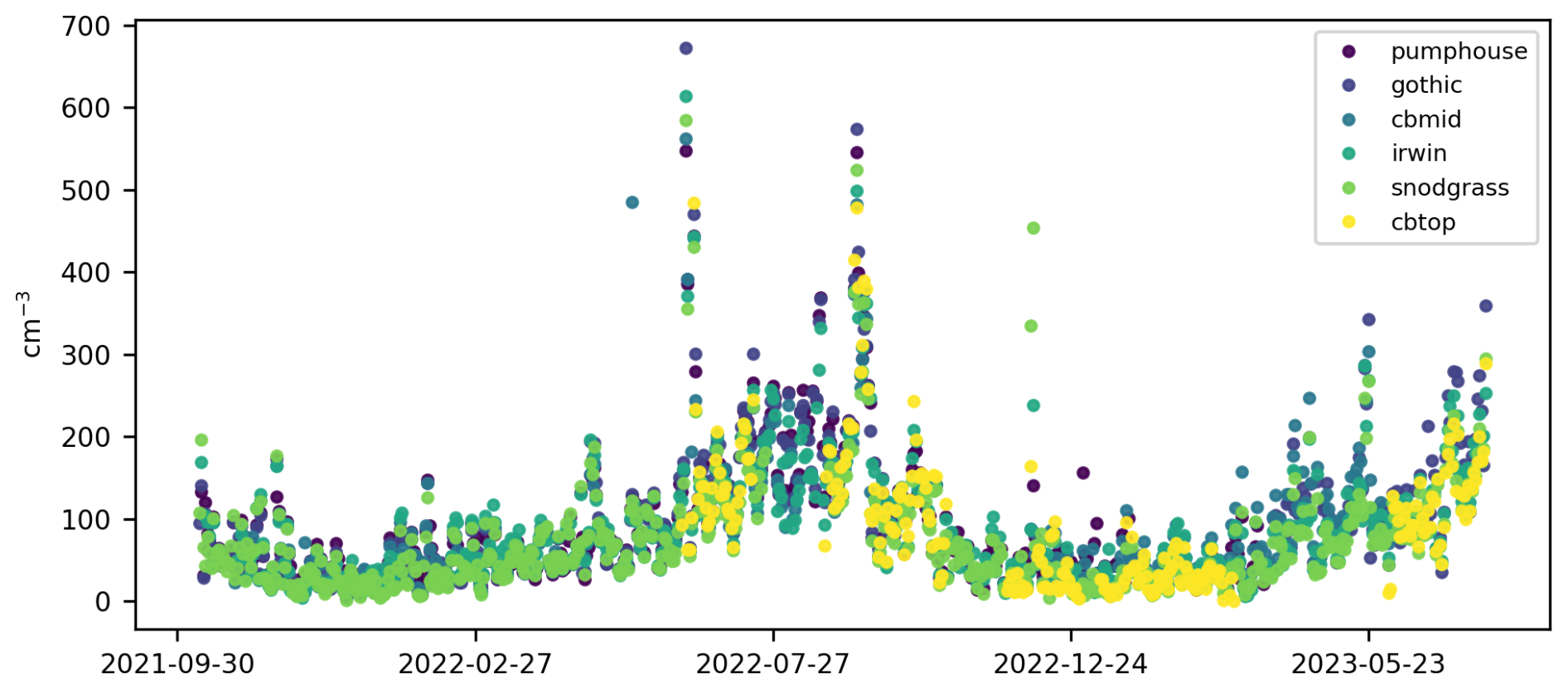
Figure 4 Time series of daily averaged concentrations of 170 nm–3.4 µm sized aerosol particles for the six sites in SAIL-Net.

The daily averaged data indicate that all the sites exhibited similar daily behavior and seasonal trends. The sites experienced higher total aerosol concentrations in the summer and lower total aerosol concentrations in the winter, consistent with the seasonal trends observed in other mountainous regions (Gallagher et al., 2011). Concentrations peaked in late summer and reached a minimum in January. However, the maximum recorded concentration occurred on 13 June 2022 at Gothic, with an average daily concentration of 672 cm⁻³, due to smoke from the Flagstaff wildfires that were burning in Arizona. Concentrations were also abnormally high in September 2022 due to biomass burning. The unique differences and trends in the data are discussed below and divided into three sections based on the scientific questions posed in the Introduction.

3.1 Seasonality and diurnal patterns

Both seasonal and diurnal cycles were observed in the POPS data. In this section, we use the time series of the network mean of the data to study the temporal variability in aerosols. The network mean at time t, N_t, is the average of the values at m sites at time t. Thus, given a time series at each site, $\mathit{\{}{x}_{i,t=\mathrm{1}},x_{i,t=\mathrm{2}},\mathrm{\dots },x_{i,t=n}\mathit{\}}$, where i is the site number, the network mean time series for m sites is given by

$$\begin{array}{}\text{(3)}& \left\{N_{\mathrm{1}},N_{\mathrm{2}},\mathrm{\dots },N_n\right\}=\left\{{\displaystyle \frac{\sum _{i=\mathrm{1}}^m{x}_{i,\mathrm{1}}}{m}},{\displaystyle \frac{\sum _{i=\mathrm{1}}^m{x}_{i,\mathrm{2}}}{m}},\mathrm{\dots },{\displaystyle \frac{\sum _{i=\mathrm{1}}^m{x}_{i,n}}{m}}\right\}.\end{array}$$

Since the network mean takes the average of the spatially dispersed sites, it removes much of the noise and variability caused by local sources or instrument drift and can be used as a proxy for a model grid cell in the region.

Most sites had gaps in their data at some point, so when one or multiple sites were missing data, the network mean was computed from the sites with available data. This choice was made to preserve as much temporal coverage as possible and to attain a clear picture of seasonal trends. For further discussion of the network mean and its ability to represent the East River watershed, see Sect. 3.3. In the following analysis, the sum of concentrations of aerosol particles between 170 nm and 3.4 µm is used, unless otherwise specified.

SAIL-Net collected data during two very different winters. The 2022 snowpack in the Gunnison River basin, of which the ERW is a part, was close to the median for the region. However, if it had not been for a large snowfall in late December 2021, the snowpack would have been well below normal. In contrast, the 2023 winter saw higher-than-normal snowfall, with snow water equivalent peaking in the 90th percentile of the 30-year median (NRCS, 2023). Despite these very different winters, the daily average aerosol concentrations for 170 nm–3.4 µm sized particles in the network mean showed similarities over the years. Figure 5 displays the network means, represented across the days of the year. The main difference between the 2 years occurred on 13 June 2022 and in the few days that followed, when the spikes in concentration were due to smoke from the Flagstaff wildfires in Arizona. The maximum recorded concentration occurred during this time. The minimum recorded concentration of the network mean occurred on 24 December 2021, with a concentration of 7 cm⁻³. This minimum was likely caused by scavenging due to the heavy snow that fell on the same date. Below, we further analyze the temporal trends in the aerosol data.

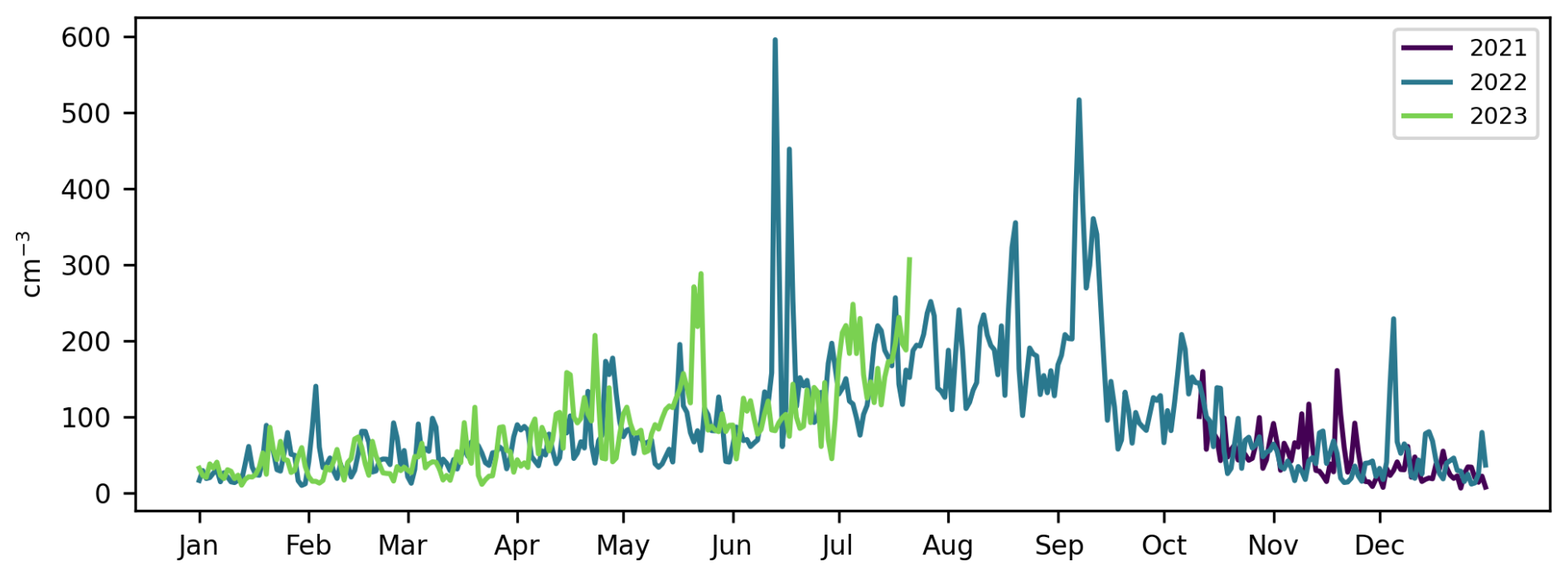
Figure 5 The network means of daily concentrations of 170 nm–3.4 µm sized aerosol particles, represented across the days of the year.

The distribution of particle sizes changed monthly and also slightly differed between the 2 years, depending on the month. Figure 6 displays the monthly average number size distribution (N vs. D_p) of aerosols, categorized by month. In general, supermicron concentrations peaked in April and were higher in March through June, primarily due to aeolian dust transported from the desert to the southwest (Skiles et al., 2015). The two spring dust seasons were noticeably different, as evidenced by the differing shapes of the number size distributions for supermicron-sized particles. According to the POPS data, supermicron concentrations increased in March and remained elevated through June 2022, whereas in 2023, April saw the highest supermicron concentrations. Submicron concentrations peaked in the summer and quickly dropped off in the fall.

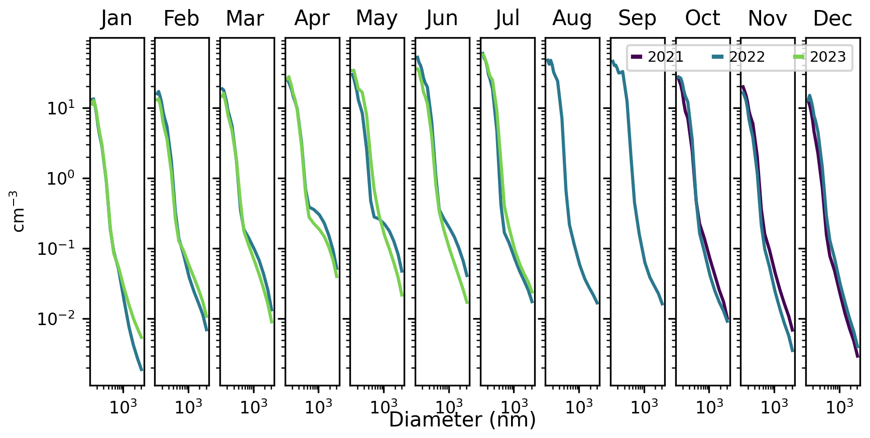
Figure 6 The number size distribution of the network means is averaged for each month. Multiple years of data are plotted where present. These plots use the full 140 nm–3.4 µm size range of the POPS instruments.

Figure 7 shows a time series of daily averaged particle size distributions for the entire measurement period. Here, we observe the seasonality of different particle sizes. Particles between 140 and 300 nm increased in the spring and early summer and peaked in late summer. There was a period in both winters, around late December and early January, when the air was extremely clean, with very few particles larger than approximately 300 nm. This figure also provides another look at the spring dust events, which were characterized by higher-than-normal concentrations of supermicron-sized particles.

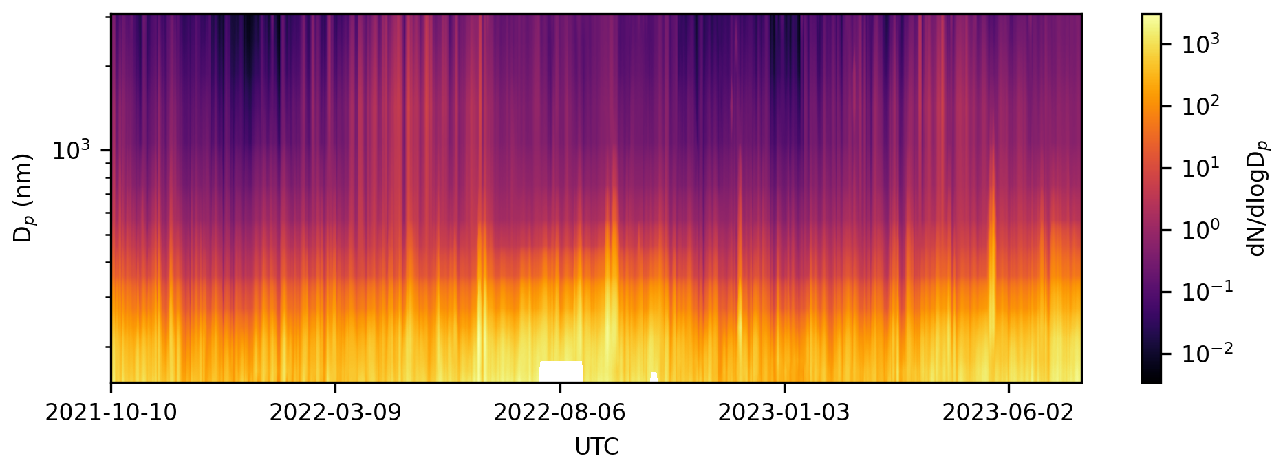
Figure 7 Time series of the measured particle size distributions of the network means. Data were averaged for each day. This plot uses the full 140 nm–3.4 µm size range of the POPS instruments.

The diurnal cycles in aerosol concentrations changed seasonally and varied between the sites. Figure 8 shows the average diurnal cycle of concentrations of 170 nm–3.4 µm sized aerosol particles, presented seasonally for each SAIL-Net site. Concentrations were averaged hourly and then grouped by meteorological season. The shaded region around each line represents the interquartile range of the seasonal data. For this analysis, we removed data from 13 to 16 June 2022 to ensure that the abnormally high concentrations caused by wildfire smoke would not affect the trend.

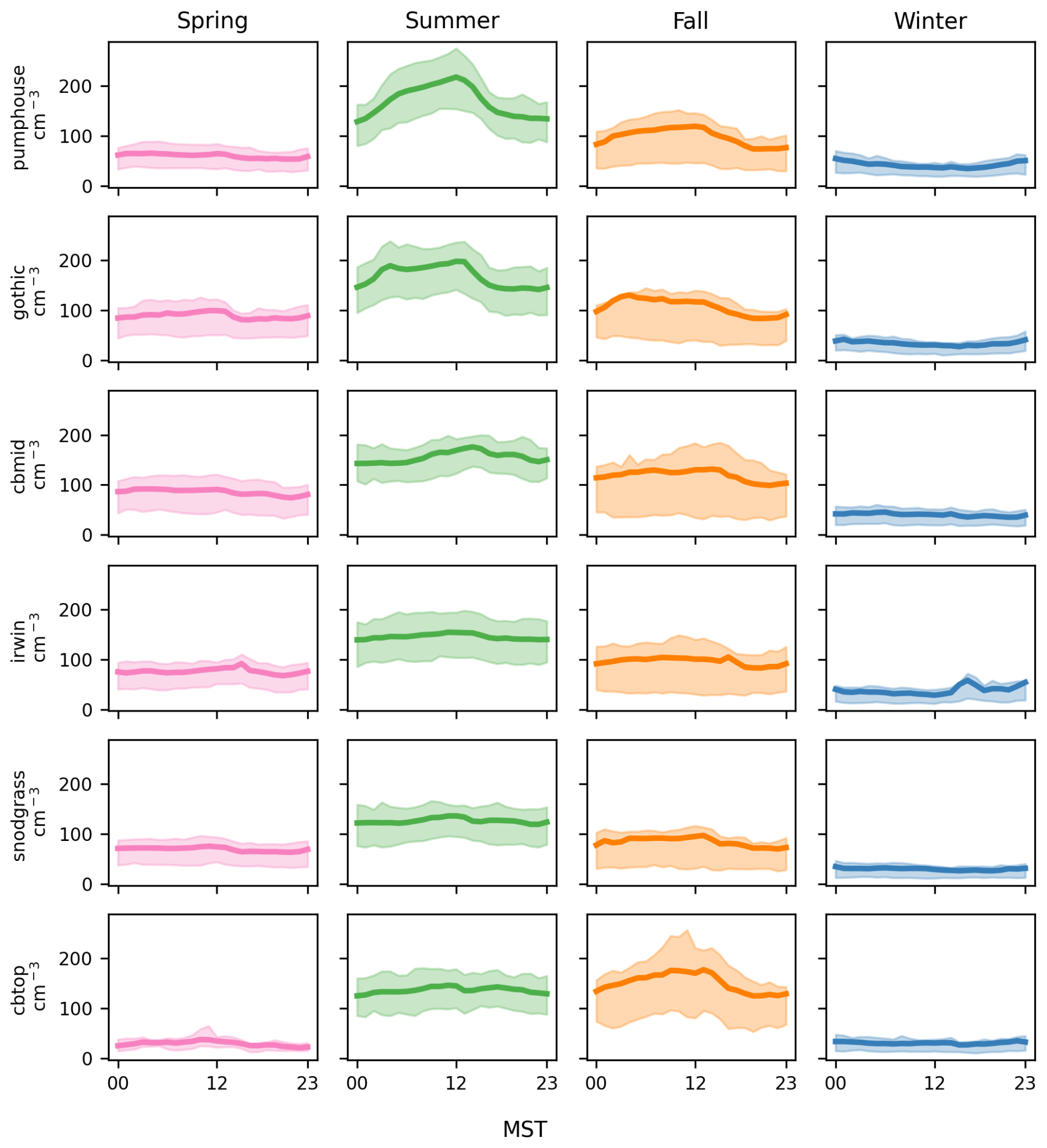
Figure 8 Daily diurnal cycles of hourly concentrations of 170 nm–3.4 µm sized aerosol particles, averaged seasonally for each SAIL-Net site. The shaded band around each line indicates the interquartile range of the seasonal data. Times have been converted to Mountain Standard Time (MST) for ease of interpretation.

The diurnal cycles were most pronounced in the summer and fall, when there were higher total aerosol concentrations. In contrast, there were minimal to no diurnal cycles observed in the winter and spring. The lack of diurnal cycles in the winter months could be partially attributed to reduced vertical mixing of the boundary layer throughout the day (Gallagher et al., 2011). Irwin does seem to exhibit some patterns in the winter and spring, with concentrations increasing in the afternoon, but we believe this increase was due to consistent snowcat and snowmobile activity around the site during these seasons.

While the diurnal cycles look different across the SAIL-Net sites, there is an underlying consistency in the daily trends for summer and fall. Aerosol concentrations tended to increase overnight and into the morning, peaking in the early afternoon. Concentrations then decreased throughout the late afternoon and evening. This behavior was especially clear at Pumphouse and Gothic in the summer, possibly due to the influence of anthropogenic activities around the sites or the unique conditions in the East River valley, where both sites were located. These observations are partially consistent with the diurnal analysis conducted by Gallagher et al. (2011) at Whistler Mountain, which studied the seasonal and diurnal patterns of CCN. They found that diurnal cycles were more distinct in the warmer months and less so in the winter. They also observed increasing CCN concentrations from 08:00 until approximately 16:00 LT (local time) as a result of new-particle formation (NPF). While this daytime increase was also observed in the SAIL-Net data, we were unable to determine whether NPF drove this increase since a POPS cannot measure particles small enough to observe it. Likely, the height of the convective boundary layer, coupled with anthropogenic activities in the nearby town of Crested Butte, drove the nighttime–midday increases in aerosol concentrations. However, more analysis is necessary to be certain.

3.2 Spatial variability

Networks of sensors are useful in cities and more polluted areas because aerosol concentrations vary dramatically over small spatial scales (Popoola et al., 2018; Caubel et al., 2019). In less populated areas, such as the ERW, there are not as many local sources of emissions. However, aerosol properties can vary with elevation change (Zieger et al., 2012). This section explores the spatial variability in the region and its relationship with elevation.

Figure 4 showed that all sites were reasonably similar on a daily timescale. However, there was still variability within the data, especially on a smaller timescale. Subdaily variability was primarily due to local emissions and the distances between the sites. We were able to identify the sources of some of this variability, and a few examples are described below.

CBMid and Irwin experienced spikes in 155–300 nm sized particles from late November to early April, which we attributed to nearby snowcat and snowmobile activity. Figure 9a illustrates these spikes over a few days with respect to the winter of 2022. The spikes at CBMid occurred during the night (local time), corresponding with the Crested Butte Mountain Resort's nightly grooming of its runs. The spikes at Irwin occurred roughly between 09:00 and 15:00 LT, corresponding with the times when snowmobiling and other winter activities took place. Concentrations at Gothic were influenced by increased anthropogenic activity in the summer. Figure 9b displays these effects in comparison to the concentrations at Pumphouse, also located in the East River valley. The road to Gothic opened at the end of May 2022, aligning with the onset of the noisy spikes at Gothic. It is unclear whether these spikes were due to road traffic or other activities near the town of Gothic, such as campfires. Variability between the sites was also due to their dispersed locations. Figure 9c displays this behavior for 13 June 2022, when smoke from the Flagstaff wildfires blew into the region. In this case, the sites reported similar concentrations with a lag between them, leading to increased variability as the plume moved into the area.

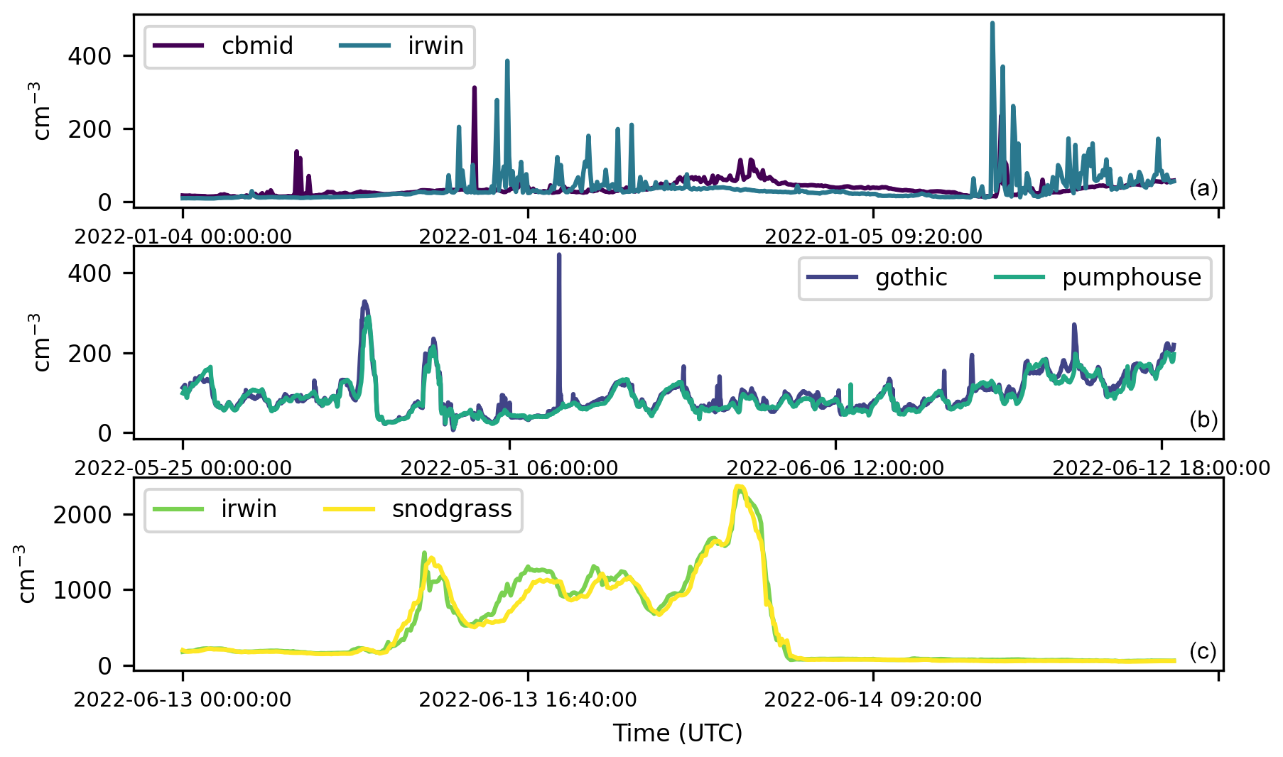
Figure 9 Examples of subdaily variability among the SAIL-Net sites. Panel (a) displays the spikes in 155–300 nm sized aerosol particles at CBMid and Irwin, which were both affected by winter snow-sport activities. Panel (b) displays the noisy spikes at Gothic, which began after Gothic Road opened for the season. Panel (c) displays a lag in total aerosol concentrations that occurred when a smoke plume moved into the region on 13 June 2022.

Beyond variability caused by local sources, we found that the variability between the sites was partially influenced by their differences in elevation, supporting the findings of Zieger et al. (2012). Figure 10 plots the average pairwise percentage difference in aerosol concentrations between two sites as a function of the elevation difference between these sites on the top row and as a function of the geographic distance between these sites on the bottom row. The percentage difference was calculated daily as the absolute difference between the two sites, divided by their average. These daily errors were then averaged over the total SAIL-Net deployment period to obtain the plots in Fig. 10. This was done for three groupings of particle sizes (170–300 nm, 300–870 nm, and 870 nm–3.4 µm), as well as for the full size range (170 nm–3.4 µm). These groupings were chosen based on the size ranges of particles that consistently exhibited similar concentrations. A linear regression was computed for each plot, and the Pearson correlation coefficient is reported at the top of each plot.

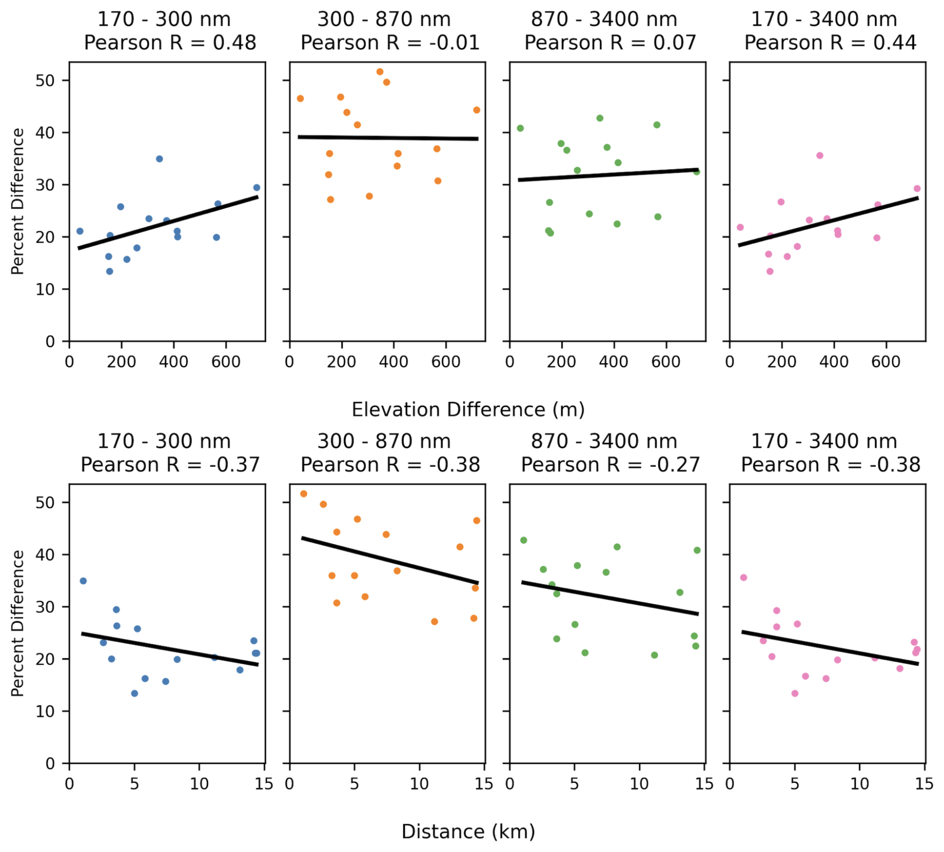
Figure 10 The plots in the top row display the average pairwise percentage difference between the sites as a function of their elevation difference. The plots in the bottom row also display the average pairwise percentage difference between the sites but this time show it as a function of the spatial distance between the sites. The average percentage difference was computed from daily averages and then averaged over the entire SAIL-Net deployment period.

For the total size range and the 170–300 nm size range, the most similar sites were Pumphouse and Gothic, with an average difference of 13.4 %. Gothic and Pumphouse were both located in the East River valley and were the two lowest-elevation sites. The most different sites, CBTop and CBMid, were geographically the closest, with an average difference of 35 %.

These plots reveal surprising results regarding the relationship between the sites. Positive Pearson correlation values of 0.48 and 0.44 for the percentage difference as a function of elevation difference – based on particles in the 170–300 nm range and the full size range, respectively – indicate that sites with closer elevations have more similar concentrations. Thus, the variability between the sites may partially be due to their differences in elevation.

We do not observe a relationship of similarity for sites that are near one another. All Pearson correlation coefficients are negative when comparing the percentage difference as a function of the difference between the sites. This result indicates that the common assumption that spatially close data are more similar does not apply here, which is particularly surprising. However, this observed negative correlation may be an artifact of the site placement. The SAIL-Net sites that were within 5 km of one another also differed by approximately 300 to 700 m in elevation and were thus more different. For the majority of SAIL-Net sites that were more than 5 km apart, their elevations were typically within 350 m of one another, so the concentrations at these sites were more similar. Thus, the positive relationship between measurement similarity and elevation may have negatively influenced the relationship between spatially proximal sites.

The variability across the sites also changed seasonally. Figure 11a shows the coefficient of variation (CV) across the sites over time. The CV represents the dispersion within a set of data. Using the daily average concentration of 170 nm–3.4 µm sized particles at each site, the data were grouped by time so that each time step provided a set of data across the sites for computing the CV. Each set was normalized using min–max scaling before computing the CV. This choice was made to account for the seasonality of the data while maintaining the relative distance between the values. Figure 11 also displays the monthly average CV, overlaid on the daily CV time series.

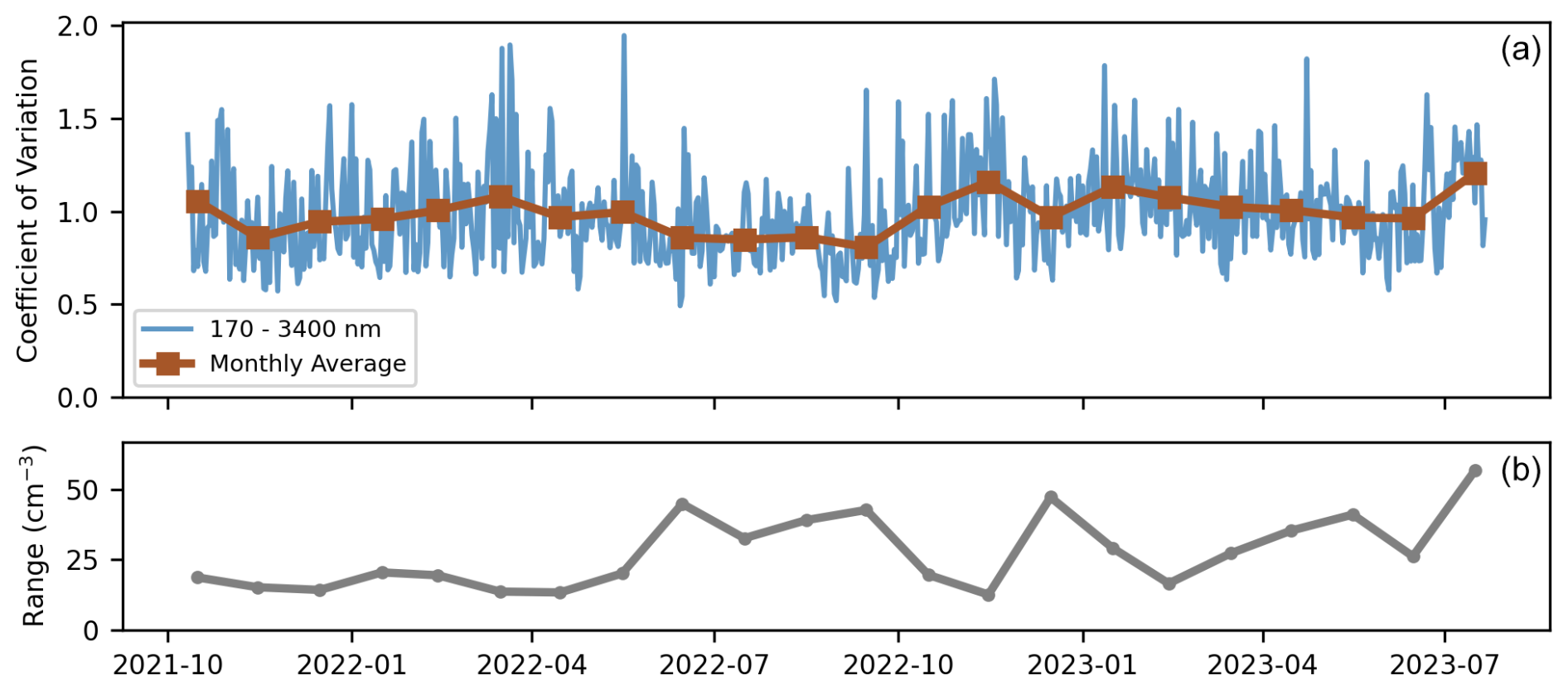
Figure 11 A time series of the coefficient of variation for daily averaged concentrations of the 170 nm–3.4 µm aerosol particles at the SAIL-Net sites is plotted in blue in panel (a). The monthly average of the CV is plotted as brown squares, overlaid on the daily CV time series. Panel (b) displays the average monthly range of concentrations between the sites.

Overall, there was fairly high variability across the sites. The average monthly CV was typically near or greater than 1, indicating that the standard deviation of the sites' measurements was close to or larger than the mean of the data. There was less variability among the sites during the summer of 2022 than in the other seasons. The variability also began trending downward as the weather warmed in 2023 but then increased in the last few weeks of deployment. We hypothesize that the increased variability in the cooler seasons may have been partially due to the impact of snow-covered ground on the daytime convective boundary layer. Adler et al. (2023) noted a low convective boundary layer over snow-covered terrain in the East River watershed and observed inversions at night. In some observations, the boundary layer was low enough for some high-elevation sites in SAIL-Net to be above it and thus for these sites to measure different aerosol concentrations than those below the boundary layer. However, another factor that likely affected the higher variability in the winter months was the low aerosol concentrations across the sites. The depths of winter experienced concentrations of less than 100 cm⁻³ on average. In such clean conditions, any local variability would amplify the differences between sites. Figure 11b displays the monthly average range of concentrations between the sites, whose values were typically lower in the winter and higher in the summer. There appears to be an inverse relationship between the monthly averaged CV and the monthly averaged ranges, indicating that despite the min–max scaling applied to the data, the number counts of aerosols in different seasons affected the computed CV. Thus, although there appears to be higher variability in the colder months, this may predominantly be an artifact of the low wintertime concentrations.

3.3 Network representation

The previous subsections highlighted the temporal and spatial variability of aerosols in the ERW. We now use these data to investigate the optimal network design for the region and determine whether a single site can accurately represent the aerosol properties of the region. This section is divided into two separate analyses. The first investigates the spatial representativeness of the sites using an analysis approach similar to that used by Asher et al. (2022) for POPSnet-SGP. The second analysis is more exploratory and utilizes the varying altitudes of the SAIL-Net sites to compare ground-based measurements with airborne measurements from tethered-balloon flights, which characterized the vertical column of air in the region.

3.3.1 Regional representation

As defined and studied by Schutgens et al. (2017), the representation error is the ability of a measurement to represent a larger area. There is often a significant difference between model estimates for a region and observed point measurements, leading to inaccuracies (Schutgens et al., 2016). The representation error quantifies how similar each site is to the network mean (Eq. 3 in Sect. 3.1). Local sources affect measurements at a single site, so it can be advantageous to average values over multiple sites to gain a more balanced picture of the region. However, if there are significant and consistent differences between the sites, the network mean can mask this variability. The representation error treats the network mean as a proxy for the true regional value and quantifies how different a single site is from the network mean. This provides meaningful insights into the usefulness of a network of sites in complex terrain by showing how different or similar each site is to this proxy.

Using the equation from Asher et al. (2022), the representation error, e_t, is the normalized difference between a site observation and the network mean for a given averaging period, t:

$$\begin{array}{}\text{(4)}& e_t={\displaystyle \frac{O_t-N_t}{N_t}}.\end{array}$$

During the POPSnet-SGP campaign in the southern Great Plains, Asher et al. (2022) found that the representation error decreased when data were averaged over longer periods. This was true for SAIL-Net. We used daily averaged data for the following analysis. The representation error was then computed for each site on every day that had valid data. As with the computation of the network mean, not all days had data for all six sites. However, in order to maximize the temporal span of the data, we computed the representation error for sites whenever possible. Since the number of sites and number of days of data were not consistent across the sites, this may have had an effect on the results of the following analysis. However, we believe that, given the approximately 600 sampling days, there were sufficient data to ensure that these missing values would not have a massive impact on the overall results.

Since the POPS data showed significant seasonal changes, with much higher concentrations in the summer than in the winter, we investigated the representation error seasonally. We grouped the daily representation errors by season, and Fig. 12 shows the results for three size ranges: the full 170 nm–3.4 µm size range, 170–300 nm, and 300 nm–3.4 µm. While the 300 nm–3.4 µm size range was broken down in the analysis in the previous section, there were so few counts of particles larger than 1 µm that the representation errors were extremely high. In general, the representation error appeared higher in the winter and lower in the summer. However, the lower aerosol concentrations across the sites in the winter likely impacted the representation error, so caution must be taken when comparing the errors across seasons.

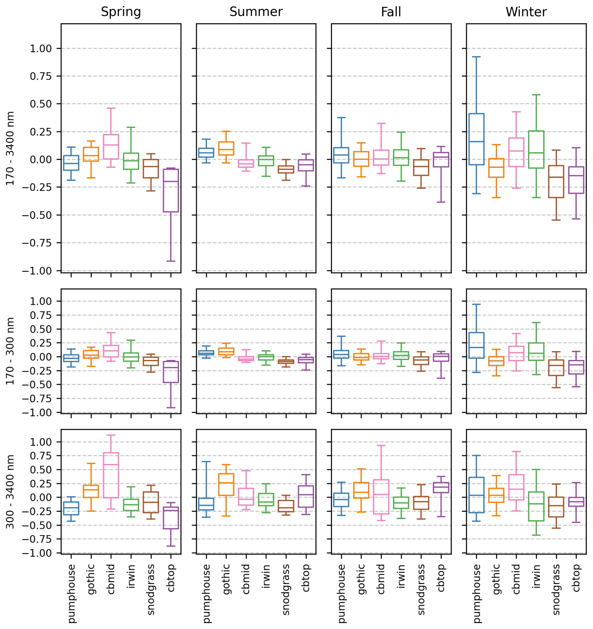
Figure 12 The representation error for each site, categorized by meteorological season and size ranges (170 nm–3.4 µm, 170–300 nm, and 300 nm–3.4 µm). The notches in each modified box plot indicate the 5th, 25th, 50th (median), 75th, and 95th percentiles.

Instead, we compared the representation errors across the sites within each season to determine the most representative site for each season and size range. The most representative site should have a median close to zero and a small range. In Fig. 12, the whiskers of the box plot mark the 5th and 95th percentiles. To determine the most representative site, we assigned a score to each site and size range by summing the median's absolute value and the data range between the 5th and 95th percentiles. Using this approach, the most representative sites for each size range were as follows:

• 170 nm to 3.4 μm. Pumphouse (spring), Irwin (summer), Gothic (fall), and Gothic (winter) were the most representative.

• 170 to 300 nm. Pumphouse (spring), Irwin (summer), Gothic (fall), and Gothic (winter) were the most representative.

• 300 nm to 3.4 μm. Pumphouse (spring), Snodgrass (summer), Pumphouse (fall), and CBTop (winter) were the most representative.

The most representative site was inconsistent across different seasons and between the three size ranges. This suggests that the aerosol properties of the region are complex and vary by season and size, meaning there is no single, consistently most representative site for the region.

One of the observations driving the deployment of SAIL-Net was that aerosol complexity is increased in mountainous terrain compared to over flat land (Zieger et al., 2012; Yuan et al., 2020; Nakata et al., 2021). The results of SAIL-Net further support this conclusion. In comparing the range of representation errors against the results of POPSnet-SGP (Asher et al., 2022), which collected data between October and March, SAIL-Net observed the same or larger errors across many of the sites in both the winter and spring. This suggests that aerosol complexity is increased in mountainous terrain since the SAIL-Net sites were more spatially dense than those in POPSnet-SGP but still observed equal or greater errors in the same season.

3.3.2 Vertical representation

The previous representation analysis quantified the ability of a single site to represent larger areas. Given the varying elevations of the sites, we also explored how representative the sites were of the vertical profile of air in the region. The six SAIL-Net sites were intentionally placed at various elevations across the ERW to cover a portion of the altitudes in the area. To quantify how representative the SAIL-Net sites were of the vertical profile of aerosols in the region, we compared our data to the data collected during tethered-balloon-system (TBS) flights that took place in the ERW during the SAIL campaign (Mei et al., 2023). The TBS flights occurred at Gothic in 2022 and at Pumphouse in 2023. Each balloon was equipped with a POPS from Handix Scientific, which allowed for easy comparison with the POPS instruments at the SAIL-Net sites.

During each TBS flight, the balloon was sent up vertically through the atmosphere. The balloon remained approximately in the same geographic location to allow for each flight to generate a profile of the vertical air column in the region, where each measurement was associated with an altitude above sea level (a_f) and a time (t_f). To compare the data from the TBS flight with SAIL-Net, we built a pseudo vertical column from the SAIL-Net sites. We did this by associating the altitude above sea level of each site (a_s) with its measured total aerosol concentration at time t_s, ignoring the geographical location of the site. Time t_s was determined using the time at which the altitude of the tethered balloon passed within 2.5 m of the altitude above sea level of the site. Mathematically, t_s was the time at which $a_s-\mathrm{2.5}<a_f<a_s+\mathrm{2.5}$. We then obtained the average of the concentrations at site s over a 1 min window around t_s and set this as the value of the pseudo vertical column for the altitude–time pair (a_s, t_s). The error between the concentration reported by the POPS on the TBS flight and the concentration at the SAIL-Net site was computed for each altitude–time pair (a_s, t_s) in the SAIL-Net vertical column.

We recognize that the pseudo vertical column generated by the SAIL-Net sites is a crude approximation of a vertical column since it does not account for the differing geographic locations of the sites and the measurements from the sites are ground-based instead of airborne. However, this approach provided a straightforward method for comparing between spatially dispersed ground-based measurements and airborne measurements. Figure 13 shows examples of TBS flight data for 13 and 14 June 2023, plotted along with the SAIL-Net vertical column. These two dates also highlight the variability in the vertical column of air between different flights. For some flights, such as the one on 13 June 2024, the column of air was well mixed, and concentrations at approximately 2800 m were within approximately 10 cm⁻³ of those at nearly 3500 m. For other flights, such as the one on 14 June 2024, the column of air was not as vertically mixed. Though not displayed here, some flights also passed through plumes at certain altitudes where concentrations momentarily spiked.

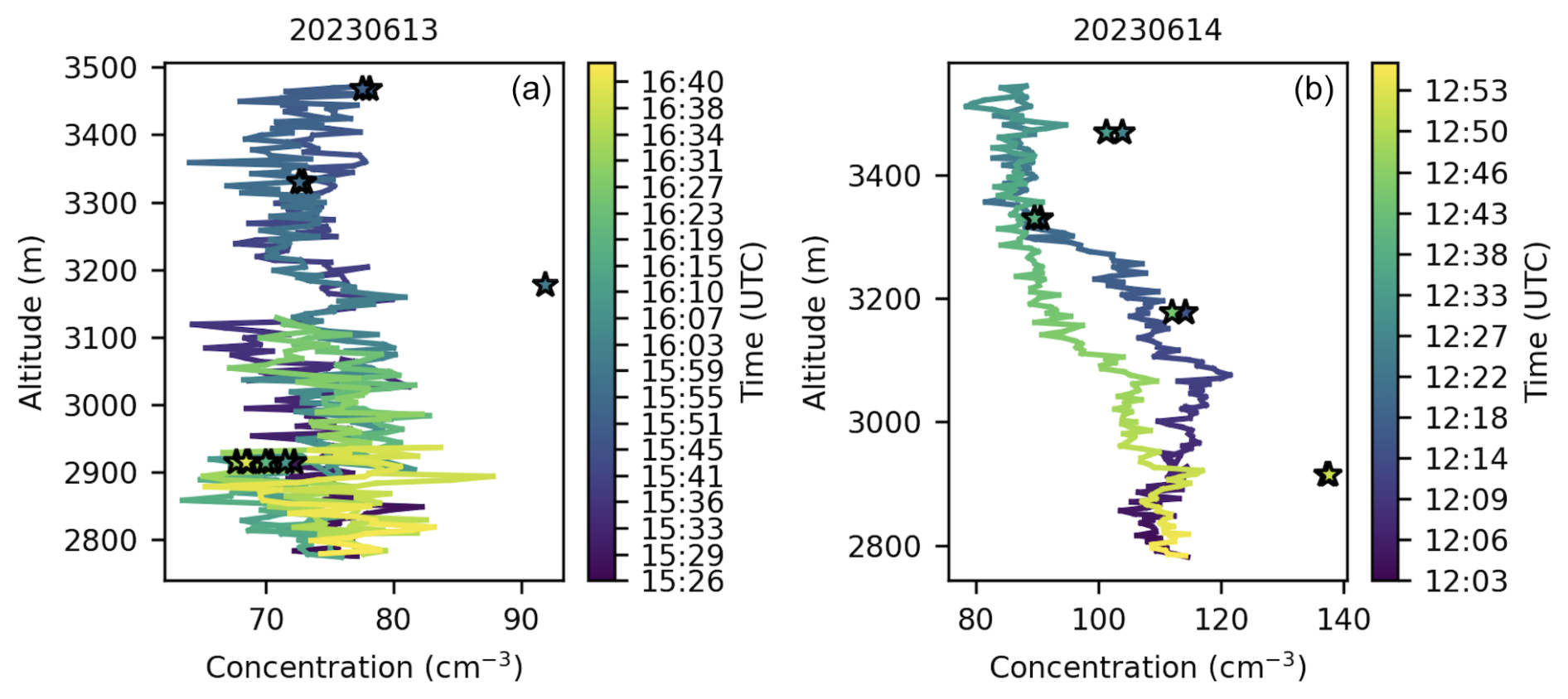
Figure 13 A visual comparison between the TBS flights on (a) 13 and (b) 14 June 2023 and the pseudo vertical column generated by the SAIL-Net sites. Each star represents a measurement in SAIL-Net's pseudo vertical column, plotted at the site's altitude above sea level. A star is placed for each instance when the TBS flight's altitude above sea level passed within 2.5 m of the altitude of a SAIL-Net site.

For each flight, we computed (1) the absolute value of the percentage difference between the vertical column of the flight and the vertical column of the sites and (2) the absolute difference between the two values. This choice was made because the seasonality of the total concentrations may have made the percentage error a less useful metric for understanding the differences in the region over time, as we saw in the previous analysis. We grouped the errors by day, even if there were multiple flights in a single day. Figure 14 displays a box plot of the absolute errors collected on each day of the flights, as well as a line plot showing the median percentage error for each day. While the TBS flights took place on more days than those shown in Fig. 14, we limited the comparison to days when the SAIL-Net vertical column was generated by at least half of the SAIL-Net sites. We chose the median because we wanted to obtain a metric that represented the typical difference between the site and the vertical column and did not want to be influenced by outliers, which were sometimes present, typically due to local sources at the ground-based sites. The median percentage error between the two vertical columns was highest in April 2023, which is not surprising given that April typically had lower total aerosol concentrations than any of the warmer months in which the balloons flew. The lowest median percentage error, 4.7 %, occurred on 13 June 2023, while the highest error, 204.3 %, occurred on 6 April 2023. Moreover, 13 June 2024 also had a low absolute difference, with a median concentration difference of 3.5 cm⁻³ and range of 15.4 cm⁻³. By contrast, 6 April 2023 had a median concentration difference of 51.5 cm⁻³, indicating that despite there being lower total aerosol concentrations in spring, there was still a significant difference between the absolute measurements. Over 75 % of the days had a median percentage error under 25 %, and more than half of the days had a median percentage error below 15 %.

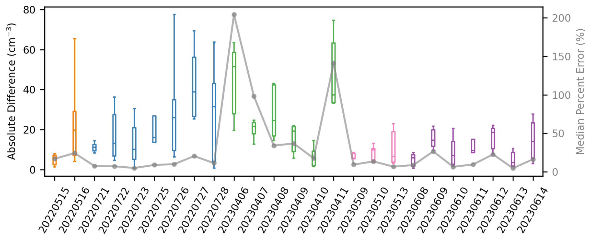
Figure 14 The daily absolute differences between the TBS vertical column and the SAIL-Net pseudo vertical column are plotted as box plots, with interquartile ranges represented by boxes and whiskers extending to the 5th and 95th percentiles. The box plots are color-coded based on the month in which the flight occurred. The median percentage error is plotted as a gray line. Each flight date is marked on the x axis in the format YYYYMMDD.

Given the difference between these measurements – i.e., the true vertical column generated by the airborne measurements and the pseudo vertical columns from the ground-based measurements – these errors were surprisingly low. This suggests that the SAIL-Net sites were able to capture the vertical profile of aerosols reasonably well, given the sample set. However, the majority of the comparison days were in the spring and summer, when there were higher total aerosol concentrations and temperatures were warmer. During these days, there was likely, in general, better mixing of the boundary layer than in winter, meaning there was less vertical variability in the air overall, as observed on 13 June 2023 (Fig. 14). There would need to be significantly more comparisons like this during different seasons and times of the day to determine whether dispersed, ground-based measurements at different elevations can sufficiently characterize the vertical column of air. These results do, however, further emphasize the relationship between aerosol variability and elevation in complex terrain.

4 Conclusions

SAIL-Net was the first network of its kind to operate in mountainous terrain and now provides a comprehensive dataset highlighting the spatiotemporal variability in PM_2.5 in complex terrain. The results of the above analysis indicate some variability between the SAIL-Net sites, which appears to be at least partially driven by the elevation of the sites. However, the differences between the sites may not be significant enough, depending on the measurements and their use cases. This conclusion would ultimately be left to the user of the data.

SAIL-Net observed seasonal and diurnal cycles in aerosol concentrations. The highest concentrations occurred in late summer, while supermicron concentrations peaked in spring, likely due to aeolian dust. Diurnal cycles were more pronounced in the warmer months, consistent with the findings of Gallagher et al. (2011). There was more variability between the sites in winter than in summer, possibly because the lower concentrations in winter made the sites more sensitive to local sources. There is also the possibility that the wintertime convective boundary layer was low enough for some higher-elevation SAIL-Net sites to be above it, which may have led to increased variability, though more work should be done here to identify the cause.

The differences in concentration between the sites were partially related to the sites' elevations, with a Pearson correlation coefficient (R) value of 0.44 linking elevation proximity to measurement similarity. This relationship between concentration and elevation was further supported by the ability of the sites to represent the vertical profile of air in the region. Comparisons between the site data and TBS flights showed that the error in the sites representing the vertical profile of air in the region was as low as 4.7 % in June 2023. However, one spring day measured an error as high as 204 %, indicating that factors beyond elevation drove the variability between the sites. The variability between the sites was inconsistent across different seasons, underscoring the potential inadequacy of a single site to consistently represent the complex terrain in the ERW. However, the similar daily trends across the sites indicate that, on a larger timescale, there is minimal variability in the region. Compared to the range of representation errors observed by Asher et al. (2022), the SAIL-Net sites experienced larger representation errors over a smaller spatial region. This result emphasizes that there is increased variability in aerosols in complex terrain and also supports the findings of Zieger et al. (2012) for the Swiss Alps.

There is future work that could be done with this dataset. While this paper focused on analyzing the variability and trends in the data, there are opportunities for modeling and further analysis. One such direction would be to combine these data with other observations to begin explaining the behaviors observed here. For example, one could explore the possible causes of increased variability in winter. Another direction would be to investigate the diurnal cycles in aerosol concentrations to understand why these concentrations decrease in the afternoon. Including data from new-particle formation and studying patterns in daily upslope and downslope winds may provide additional clarity. The comparison of the site data against measurements from tethered-balloon flights in the region showed surprisingly similar results and may warrant further investigation to explore how a network of ground-based sensors in complex terrain could sufficiently characterize the vertical column of air in the region.

One of the primary drawbacks of these data was the presence of gaps and possible remaining instrument differences. The gaps in the data made it impossible to consistently compute a daily representation error for all six sites. This may have affected the results of the representation and network analysis since the daily representation error was computed only from the sites that had data available each day. However, we believe that these possible errors do not affect the overall seasonal trends or the relationship between concentrations and elevations that we observed. While the data were post-corrected using monthly PSL checks, there may not have been frequent enough checks to correct for all errors and drift. For example, unlike in POPSnet-SGP, where two POPS instruments were colocated to monitor accuracy, only one POPS was stationed at each site. However, we are still confident that the behavior observed at individual sites and between the sites was predominately attributed to true measurements and not instrument differences.

This initial analysis supports the claim that aerosol concentrations are more variable both spatially and temporally in regions of complex terrain than over flat land. However, the similar trends in the data from the daily averages shown in Fig. 4 indicate that there is consistency across the region on a daily or larger timescale. This suggests that, depending on the desired accuracy of modeling efforts in the region, it may be necessary to take this variability into account. Furthermore, the change in variability across seasons suggests that models may not retain the same accuracy over time. These data provide valuable insights into aerosol variability in mountainous terrain and serve as a blueprint for future measurement networks in similar regions.