Characterization of atmospheric water-soluble brown carbon in the Athabasca oil sands region, Canada

Extensive industrial operations in the Athabasca oil sands region (AOSR) (Alberta, Canada) are a suspected source of water-soluble brown carbon (WS-BrC), a class of light-absorbing organic aerosols capable of altering atmospheric solar-radiation budgets. However, the current understanding of WS-BrC across the AOSR is limited, and the primary regional sources of these aerosols are unknown. During the summer of 2021, active filter-pack samplers were deployed at five sites across the AOSR to collect total suspended particulate matter for the purpose of evaluating WS-BrC. Ultraviolet–visible spectroscopy and fluorescence excitation–emission matrix (EEM) spectroscopy, complemented by parallel factor analysis (PARAFAC) modelling, were employed for sample characterization. Aerosol absorbance was comparable between near-industry and remote field sites, suggesting that industrial WS-BrC exerted limited influence on regional radiative forcing. The combined EEM–PARAFAC method identified three fluorescent components (fluorophores), including one humic-like substance (C1) and two protein-like substances (C2 and C3). Sites near oil sands facilities and sample exposures receiving atmospheric transport from local industry (as indicated by back-trajectory analysis) displayed increased C1 and C3 fluorescence; moreover, both fluorophores were positively correlated with particulate elements (i.e. vanadium and sulfur) and gaseous pollutants (i.e. nitrogen dioxide and total reduced sulfur), indicative of oil sands emissions. The C2 fluorophore exhibited high emission intensity at near-field sites and during severe wildfire smoke events, while positive correlations with industry indicator variables suggest that C2 likely reflected both wildfire-generated and anthropogenic WS-BrC. These results demonstrate that the combined EEM–PARAFAC method is an accessible and cost-effective tool that can be applied to monitor industrial WS-BrC in the AOSR.

1 Introduction

Water-soluble brown carbon (WS-BrC) represents a class of organic aerosols capable of absorbing light within the ultraviolet (UV) and visible (Vis) wavelength ranges (Basnet et al., 2024; Lin et al., 2012; Stone et al., 2009). Chemical species within the WS-BrC fraction are classified as chromophoric dissolved organic matter (CDOM), which generally consists of polymerized, aromatic humic-like substances (HULISs) and lower-molecular-weight protein-like substances (PRLISs). Both HULISs and PRLISs represent broad chemical groups named according to their chemical and optical similarities to humic matter and proteins found in terrestrial, aquatic, and atmospheric environments (Dey and Sarkar, 2024; Duarte et al., 2007; Laskin et al., 2015).

Due to their light-absorbing properties and capacity as cloud condensation nuclei, WS-BrC particles can influence planetary albedo and solar-radiation budgets (Zhou et al., 2023; Liu et al., 2015) and, as such, have been recognized as an influential factor in climate change research (Chakrabarty et al., 2016; Gustafsson et al., 2009). Moreover, soluble BrC has been found to play an important role in atmospheric reaction chemistry (Jiang et al., 2012) and can be detrimental to human health (Li et al., 2017; Ma et al., 2019). Biomass and fossil fuel combustion are dominant sources of atmospheric WS-BrC, including HULISs and PRLISs (Claeys et al., 2012; Wu et al., 2019; Zeng et al., 2022); however, biogenic emissions, soil dust, and industry can also contribute to the primary and secondary formation of these organic aerosols (Spranger et al., 2020; Wu et al., 2019).

Industrial operations in the Athabasca oil sands region (AOSR) in northeastern Alberta, Canada, are a substantial source of atmospheric particulate matter (PM) (Giesy et al., 2010; Landis et al., 2017; Liggio et al., 2016). Open-pit-mining activities, haul road dust, dry tailings, vehicle exhaust, and upgrading facilities are sources of organic-containing PM (Giesy et al., 2010; Zhang et al., 2016), while volatile precursor emissions from flue-gas stacks and exposed bitumen contribute to the formation of secondary organic aerosols (Liggio et al., 2016). Organic PM generated from oil sands (OS) activities consists of a diverse range of chemical species, including polycyclic aromatic compounds (PACs; Bari and Kindzierski, 2018; Liggio et al., 2016; Liggio et al., 2017), oxygenated polycyclic aromatic hydrocarbons (Jariyasopit et al., 2021), naphthenic acids (Yassine and Dabek-Zlotorzynska, 2017), and organic matter linked to surface soil and overburden dust (Wang et al., 2015). An unresolved fraction of these emissions contain relatively water-soluble species (Arp et al., 2014; Josefsson et al., 2015; Marentette et al., 2015), which can contribute to the WS-BrC fraction, partially due to their conjugated structures (Stedmon and Nelson, 2015).

Relatively little is known about the abundance and composition of WS-BrC in the AOSR airshed, nor is it well understood how local industry contributes to the CDOM fraction. Considering the magnitude of sources in the region, OS emissions likely contribute to WS-BrC, which, in turn, may influence radiative forcing on a broad scale. The established toxicity and environmental mobility of water-soluble organic pollutants (Lemieux et al., 2008; Lundstedt et al., 2007) provide a clear incentive for monitoring these species throughout the AOSR; however, the diversity of WS-BrC chemical formulae has posed a challenge to regional monitoring efforts due to the high operational costs of typical mass spectrometry methods (Frysinger et al., 2003).

Ultraviolet–visible (UV–Vis) spectroscopy is commonly employed to characterize the bulk properties of environmental CDOM. Moreover, a sizable fraction of WS-BrC consists of fluorescent dissolved organic matter (Laskin et al., 2015), which can be evaluated through the application of excitation–emission matrix (EEM) spectroscopy. Complex EEM datasets can undergo processing via parallel factor analysis (PARAFAC), a multivariable model that identifies fluorescent components (fluorophores) reflective of organic compounds with shared optical properties. Fluorescence EEM spectroscopy and PARAFAC modelling have been successfully used to identify WS-BrC originating from a variety of biogenic and anthropogenic sources (Harsha et al., 2023; Wu et al., 2019; Zito et al., 2019).

In this study, we evaluated WS-BrC quality in the AOSR and assessed the influence of OS activities on the organic PM fraction through the application of UV–Vis and fluorescence spectroscopy techniques. During the summer of 2021 (19 July–10 August), active filter-pack samplers were deployed at five sites throughout the study region to collect atmospheric PM for optical and chemical analysis. Fluorescence analysis of local reference materials and back-trajectory modelling were used to assist with source identification, while partial least-squares regression (PLS-R) analysis was employed to characterize individual fluorophores generated by the PARAFAC model.

2 Methods

2.1 Study area and sampling sites

The AOSR is situated within the Boreal Plains ecozone, where peatlands and boreal forests are dominant landscape features. Largely due to its northern inland geographical location, the region typically experiences warm summers and cold, dry winters (ECCC, 2024). Beneath the boreal landscape lies the Athabasca oil sands deposit, the world's largest known bitumen reserve, which covers a surface area of ∼ 140 200 km². Oil and gas companies such as Syncrude, Suncor, and Imperial Oil have established industrial facilities on top of these deposits to extract bitumen and upgrade it into refined materials, such as crude oil. Major OS facilities are located along the eastern and western banks of the Athabasca River (which flows north through the AOSR) as the Athabasca bitumen layer is close to the surface in these areas. The largest municipalities in the region are Fort McMurray and Fort McKay; the former is located ∼ 50 km south of the major OS operations, while Fort McKay sits along the western bank of the Athabasca River, situated between several major industrial facilities (Fig. 1).

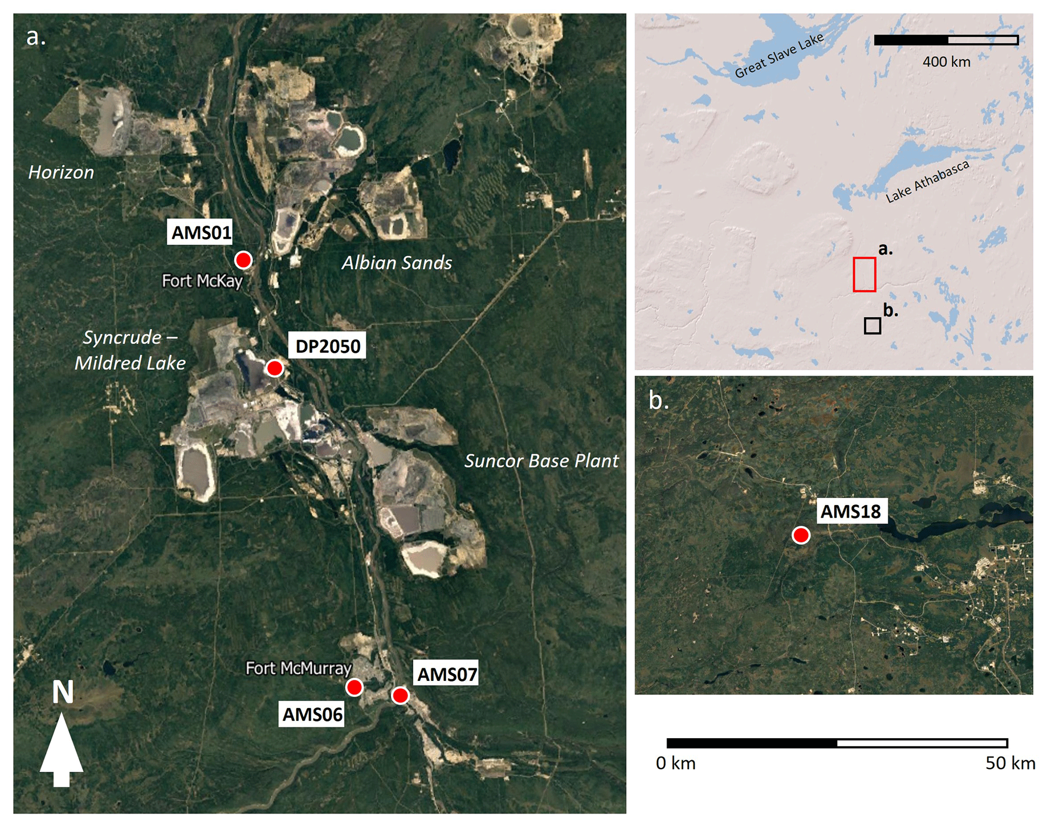
Figure 1 Distribution of active-sampler sites (red circles) throughout near- and mid-field (a), as well as far-field (b), study regions. Nearby communities (Fort McMurray, Fort McKay) and major active oil sands facilities are shown (© Google Maps 2024). The map on the top right displays the locations of the two regions on a broader spatial scale (ESRI 1995–2024).

The Wood Buffalo Environmental Association (WBEA; https://wbea.org, last access: 25 June 2024) operates an extensive network of continuous air quality monitoring stations and atmospheric deposition monitoring plots throughout the AOSR. Between 19 July and 10 August 2021, active filter-pack systems for this study were co-deployed at five WBEA sites across the AOSR to collect back-to-back 48 h exposures. Two of these fence-line sites – the Mildred Lake deposition plot (DP2050) and the Bertha Ganter station (AMS 01) – were located in close proximity to OS facilities (< 1 and < 5 km away, respectively), consisting of tailing ponds, open-pit mines, haul roads, and upgrading facilities. A second set of stations – the Patricia McInnes station (AMS 06) and the Athabasca Valley station (AMS 07) – were situated in community locations > 50 km south of major OS operations, while a final background station – Stony Mountain (AMS 18) – was located ∼ 150 km south of the OS operations (Fig. 1). Differences in observations between the stations thus allowed us to infer sources associated with OS operations versus other activities. The selected WBEA stations continuously monitored a variety of air quality and meteorological data, including data on sulfur dioxide (SO₂), total reduced sulfur (TRS), nitrogen oxide (NO), nitrogen dioxide (NO₂), total hydrocarbons (THCs), carbon monoxide (CO), fine particulate matter (PM_2.5), wind speed, wind direction, temperature, and relative humidity.

During 2021, 4.30 × 10⁶ ha of land across Canada was burned by wildfires, exceeding the 10-year annual average of 2.73 × 10⁶ ha from 2013 to 2022 (Canadian Interagency Forest Fire Centre, 2025). As a result of the increased fire magnitude, substantial portions of western Canada were periodically blanketed in smoke plumes during the study period. Wildfire emissions are a substantial source of atmospheric PM and BrC (Chen and Bond, 2010; Guan et al., 2020), which can contain aromatic pollutant species with fluorescent properties (Veselovskii et al., 2020). To account for the potential influence of wildfire emissions on observed fluorescence, the temporal variability in PM_2.5 was assessed at each WBEA monitoring station to identify sampling periods with high levels of fire smoke transport.

2.2 Active sampling

Active samplers consisted of a 15 L min⁻¹ vacuum pump connected to an in-line flow meter and a filter-pack cartridge inlet. These systems were directly powered through an alternating current (AC) outlet available at the WBEA monitoring stations, while a 12 V marine battery served as the power supply for a 7.5 L min⁻¹ vacuum pump at the off-grid DP2050 deposition plot.

The filter-pack cartridges used in this study were obtained through the Norwegian Institute for Air Research (NILU; http://www.nilu.no, last access: 4 June 2024) and consisted of two threaded compartments that housed pre-combusted quartz fibre filters (diameter: 47 mm; aerosol retention: 0.3 µm), designed to collect total suspended particulate (TSP) matter. After each exposure, filters were placed in a petri dish, triple-sealed in Ziploc^® plastic bags, and stored at −20 °C until analysis. In total, 44 filter-pack samplers were successfully deployed during the field campaign (each with a 48 h exposure), with the breakdown by site including 11 samplers at AMS 01 and Mildred Lake, 10 at AMS 06, 8 at AMS 18, and 4 at AMS 07 (Fig. S1 in the Supplement). During the study period, 5 of the 44 samples were collected as duplicates through the deployment of two sampling units. Five additional quartz fibre filters were allocated as field blanks during the study period and were stored in a similar manner to the exposed filters.

Prior to the field survey, all components of the filter-pack cartridge were individually rinsed with reverse-osmosis water and subsequently soaked in a 2 M hydrochloric acid (HCl) bath for 12 h, after which the sampler parts were rinsed with ultrapure lab water (Milli-Q). In the field, the filter-pack cartridges were soaked in baths of Milli-Q water between exposures. To control for potential filter contamination between exposures, field blanks were loaded into select washed cartridges (as if to collect a sample) and subsequently removed.

Following exposure, a 20 mm diameter subsection of the filter was removed using a circular punch and extracted in conical vials containing 50 mL of Milli-Q water. Sample vials were inverted three times, placed in an ultrasonic bath for 1 h, and filtered using a 0.45 µm nylon filter. Filtered samples were stored at ∼ 4 °C and underwent optical analysis within 12 h of the initial extraction. A 0.5 mL aliquot was used for the determination of anionic species (Cl⁻, ${\mathrm{NO}}_{\mathrm{3}}^{-}$, and ${\mathrm{SO}}_{\mathrm{4}}^{\mathrm{2}-}$) via ion chromatography (Dionex ICS-1100), while a separate 10 mL aliquot was acidified (2 % HNO₃) and sent to the Water Quality Centre at Trent University (Peterborough, Ontario, Canada) for the determination of dissolved elements (Na, Mg, P, S, K, Ca, V, Cr, Mn, Fe, Zn, and Sr) using an Agilent 8800 triple-quadrupole inductively coupled plasma mass spectrometer (Tables A1 and A2). Additional details regarding instrument configuration and measurement parameters are available in Appendix A. A filtered 20 mL aliquot was used for the determination of water-soluble organic carbon (WSOC), dissolved inorganic carbon (DIC), and total dissolved nitrogen (TDN) via a Shimadzu TOC-V analyzer. The remaining filtered solution was adjusted to a pH value of ∼ 6.5 using 0.1 M sodium hydroxide (NaOH) or HCl to limit the influence of variable sample pH on WS-BrC optical properties (Lakowicz, 2006). Blank samples were used to determine the method detection limits (MDLs), which were calculated as the standard deviation of the blank samples multiplied by the t value for the 99.0 % confidence critical value (3.747).

Measured analytes from the filter extracts were converted to time-integrated atmospheric concentrations using the following equation:

$$\begin{array}{}\text{(1)}& C={\displaystyle \frac{(C_{\mathrm{e}}-C_{\mathrm{b}})\times V_{\mathrm{e}}}{V_{\mathrm{a}}}}\times A_{\mathrm{f}}\times \mathrm{1000},\end{array}$$

where C is the atmospheric concentration (ng m⁻³); C_e is the analyte concentration (µg L⁻¹) in the filter extraction solution; C_b is the analyte concentration in the field blank extraction solution; V_e is the extraction solution volume (litres); V_a is the volume of air sampled (m⁻³); and A_f is the surface area ratio (5.52), accounting for the 20 mm filter cutout.

2.3 UV–Vis spectroscopy

Absorbance was measured across a wavelength (λ) range of 200 to 800 nm (at 1 nm intervals) using a Cary 100 UV–Vis spectrophotometer from Agilent Technologies. Filter extracts were allowed to warm to room temperature (∼ 21 °C) and were subsequently placed in a 1 cm (3.5 mL) Hellma Suprasil^® quartz cuvette (Hellma 101-QS) for analysis. A blank sample of Milli-Q water was first used to establish an instrument baseline. For cleaning, the cuvettes were soaked in a 2 M HCl bath for 10 min and subsequently rinsed with Milli-Q water and 95 % ethyl alcohol, followed by a final rinse with Milli-Q water. The aerosol light absorption coefficient (Abs_λ; m⁻¹) at wavelength λ was calculated using the following equation (Wu et al., 2019):

$$\begin{array}{}\text{(2)}& {\mathrm{Abs}}_{\mathit{\lambda }}=(a_{\mathit{\lambda }}-a_{\mathrm{700}})\times {\displaystyle \frac{V_{\mathrm{w}}}{V\times l}}\times \ln \left(\mathrm{10}\right),\end{array}$$

where V_w refers to the volume (millilitres) of the filter extraction, V is the volume of air sampled (m³) during the field exposure, l is the optical path length (centimetres), and a_λ and a₇₀₀ represent the absorbance at wavelengths λ and 700 nm, respectively. Absorbance at 700 nm is used as a reference to account for baseline drift. The light absorption coefficient at 365 nm (Abs₃₆₅) is frequently referenced as a proxy for BrC in the literature (Laskin et al., 2015; Wu et al., 2019) and is subsequently used to calculate the mass absorption efficiency (MAE₃₆₅; m² g C⁻¹) via the following equation (Wu et al., 2019):

$$\begin{array}{}\text{(3)}& {\mathrm{MAE}}_{\mathrm{365}}={\displaystyle \frac{{\mathrm{Abs}}_{\mathrm{365}}}{C_{\mathrm{a}}}},\end{array}$$

where C_a is the atmospheric concentration of WSOC (µg C m⁻³), obtained using Eq. (1). Both Abs₃₆₅ and MAE₃₆₅ are frequently used in the literature to assess the radiative-forcing potential of BrC aerosols (Dong et al., 2024; Yue et al., 2019).

2.4 Fluorescence spectroscopy and PARAFAC

The combined EEM–PARAFAC method is commonly used to evaluate the optical and structural characteristics of environmental CDOM since this modelling technique can identify the excitation and emission peaks of multiple distinct fluorophores (i.e. HULISs and PRLISs) within EEM scans (Harsha et al., 2023; Wu et al., 2019). Fluorescence analysis was conducted using a Cary Eclipse spectrophotometer set to a three-dimensional EEM scan and signal-to-reference ($S/R$) acquisition modes. Sample aliquots were placed in a 1 cm (3.5 mL) quartz cuvette (Hellma 101-QS) for analysis. Excitation (λ_Ex) and emission (λ_Em) scans (both measured at 5 nm intervals) ranged from 200–450 and 250–600 nm, respectively. A Milli-Q water blank was first measured to zero the fluorometer, after which subsequent blanks were scanned every five samples. During each day of the analysis, a set of quinine sulfate standards were prepared to create a calibration curve (1–100 ppb of quinine sulfate in 0.5 M sulfuric acid) in order to convert fluorescence intensity measurements into quinine sulfate units (QSU) (Sui et al., 2017). To minimize the potential influence of the inner filter effect (IFE) on the fluorescence spectrum, all filter extracts were confirmed to have an absorbance value < 0.05 at 270 nm (Trubetskoj et al., 2018).

Fluorescence data were processed using the R package staRdom, which was used for blank and spectrum correction (Pucher et al., 2019, 2023). Inner-filter-effect corrections were applied to individual EEMs using the built-in IFE function and corresponding sample absorbance values (measured with a Shimadzu spectrophotometer). Rayleigh and Raman light scattering bands were removed from each sample EEM, and the empty cells were filled in using the “eem_interp” function. The fluorescence intensity data were then divided by the corresponding extraction solutions and air volumes to convert quinine sulfate units (QSU) into quinine sulfate units per cubic metre (QSU m⁻³) (Deng et al., 2022). The EEM dataset displayed limited fluorescence within the 540–600 nm emission and 400–450 nm excitation wavelength ranges; thus, these regions were removed prior to PARAFAC modelling. Using the staRdom package, a PARAFAC model was employed to decompose the three-dimensional EEM data array (X_ijk) into a score matrix (A) and two loading matrices (B and C), with corresponding trilinear elements (a_if, b_jf, and c_kf) (Bro, 1997). This decomposition can be expressed as follows:

$$\begin{array}{}\text{(4)}& x_{ijk}=\sum _{f=\mathrm{1}}^F{a}_{if}{b}_{jf}{c}_{kf}+e_{ijk}.\end{array}$$

Score values for a_if represent the relative fluorescence intensity of fluorophore f in sample i. The elements b_jf and c_kf represent the modelled emission (j) and excitation (k) loadings (i.e. wavelength coordinates) of f, while F represents the total number of modelled fluorophores. Utilizing the residual element e_ijk, the PARAFAC model applies an alternating least-squares optimization technique to find the function that best approximates the dataset (Bro, 1997).

The appropriate number of modelled components (model rank) was selected based on four validation tools, including (1) visual peak inspection, (2) EEM residual plots, (3) split-half analysis, and (4) core consistency (CC). Visual inspection provides an initial check to confirm that the modelled components exhibit well-defined emission peaks, suggesting that the spectra represent a distinct fluorophore or a group of similarly fluorescing species. The model residuals corresponding to each sample (e_ijk) can be plotted as a function of λ_Ex and λ_Em. These plots can be visually inspected to identify potential peaks, where a high abundance of such features across the dataset would indicate that the model rank is not representative of the array (Driskill et al., 2018; Murphy et al., 2014). Split-half analysis involved dividing the EEM dataset into a set of four equally sized groups, where independent PARAFAC models were generated for each subgroup and subsequently compared to measure the similarity using the Tucker congruence coefficient (TCC; Pucher et al., 2019). A high TCC similarity score (∼ 1) signalled that the model was representative of the true variation within the fluorescence dataset. The model rank with the highest TCC score was most likely the appropriate selection (Bro, 1997; Stedmon et al., 2003). Core consistency is a measure of the regression between the three-way array of the PARAFAC model and the core array of the Tucker3 model, generated from the corresponding EEM data. A CC score between 90 % and 100 % indicates a strong model, while values ≤ 50 % suggest a problematic output. Generally, the largest model rank should be selected prior to a dramatic decline in CC (Bro and Kiers, 2003).

The sample score values assigned to each individual fluorescent component (a_if) were reported according to the maximum fluorescence value (F_MAX; QSU m⁻³). To account for the potential influence of bulk dissolved organic matter (DOM) fluorescence on individual fluorophore emission intensities (due to variations in DOM concentration between samples), modelled-component F_MAX values were divided by sample WSOC concentrations (µg C m⁻³) to normalize the component fluorescence.

2.5 Environmental reference materials

A variety of environmental reference materials representative of dominant TSP emission sources from the OS were collected for EEM analysis, including (a) dust from an unpaved road near the AMS 01 observation site (composite grab sample), (b) dust from a heavily trafficked unpaved road near the DP2050 observation site (composite grab sample), (c) raw-bitumen ore from the Athabasca deposit, and (d) dry mature fine tailings (MFTs) from the AOSR (composite industrial sample from InnoTech Alberta). Dry road dust and MFTs were sieved to < 2 mm to remove coarse material (Lanzerstorfer and Logiewa, 2019), while raw bitumen was too viscous to be sieved. Each reference material was extracted in Milli-Q water and diluted to achieve a WSOC concentration of ∼ 1.0 mg C L⁻¹ and an absorbance value of < 0.05 at 270 nm (to match the filter extracts). Sample extracts were adjusted to a pH value of ∼ 6.5 using 0.1 M NaOH or HCl (to match the pH of the BrC extracts) and then stored at ∼ 4 °C prior to optical analysis.

2.6 Data analysis

Variability in sampler observations was assessed by calculating the relative percentage difference (RPD; expressed as a percentage) from duplicate filter-pack exposures. Data displayed a non-normal distribution, as determined via the Shapiro–Wilk test (α < 0.05); thus, non-parametric statistical tests were employed for subsequent analysis. Median values were used as a measure of central tendency, while data variability was evaluated using normalized median absolute deviation. Bivariate associations between measured TSP analytes and continuous pollutants were evaluated via Spearman's rank-order correlation test, and the Kruskal–Wallis test was used to determine significant differences between sampling locations.

Partial least-squares regression (PLS-R) analysis was applied to assist with fluorescent-component characterization (Kothawala et al., 2014). Partial least-squares analysis is a multivariable regression technique that is effective at decomposing large numbers of collinear predictor (X) variables into a smaller set of uncorrelated orthogonal components (Eriksson et al., 2013). The PLS-R model attempts to explain the maximum variability between X variables and response (Y) variables through a least-squares regression method. Modelled fluorescent-component values (QSU m⁻³) were assigned as Y variables, while additional elements (WSOC, DIC, and TDN) were designated as X variables. The appropriate number of components was determined via internal cross-validation, where a random subset of samples (∼ 10 % of the dataset) were removed from the training dataset to evaluate the model. The resulting comparisons were evaluated based on the model rank's cumulative goodness of fit, i.e. its explained variation (R²Y), and cumulative goodness of prediction (Q²Y). The relative influence of X variables on each component was interpreted using “variable influence on projection” (VIP) scores, where values ≥ 1 signified a highly influential predictor variable (Eriksson et al., 2013). The spatial proximity of variable loadings served as a visual indicator of X- and Y-variable associations, while the variable distance from the origin indicated the level of correlation with each component.

2.7 Trajectory analysis

The atmospheric transport model HYSPLIT (Stein et al., 2015) was applied to evaluate source–receptor relationships within the study region. Meteorological data available through the Global Data Assimilation System were employed to generate bihourly backward wind trajectories (with an arrival height of 10 m above ground level) spanning the duration (∼ 48 h) of the active-sampler exposures at the individual sites (i.e. 24 back trajectories per exposure). The resulting trajectory data were overlaid onto OS facilities (polygons representing tailings, open-pit mines, and plant site boundaries) to explore the influence of industrial sources on observed TSP fluorescence. Using these spatial data, the relative frequency of back trajectories intersecting OS facility boundaries (T_OS; expressed as a percentage) during each exposure was calculated to further explore source–receptor relationships. The frequency method counts the number of times air trajectories intersect each individual grid point (0.5° × 0.5°) in the model domain and then normalizes that sum by the total number of modelled trajectories (expressed as a percentage). It should be noted that the trajectory estimates do not account for the influence of vertical mixing and lateral diffusion on pollutant transport.

Through the Canadian National Fire Database, spatial data representing the boundaries of Canadian wildfires active during the study period (19 July–10 August) were used to evaluate the potential influence of pyrogenic sources on observed fluorescence. Using the same Global Data Assimilation System meteorological datasets as before, additional HYSPLIT backward-trajectory frequency plots were modelled to evaluate atmospheric transport patterns during multi-day wildfire smoke episodes.

3 Results

3.1 Meteorology and continuous-pollutant summary

Limited variation in relative humidity occurred between the monitoring stations during the study period, with median values ranging from 69.8 % to 71.8 % (Table 1). The AMS 01, AMS 06, and AMS 07 stations experienced prominent winds blowing from a range of directions (excluding NE–E) during the study period, while S–W winds were dominant at AMS 18. Wind speeds were higher at AMS 06, while colder temperatures were recorded at AMS 18. Moreover, the background station received a larger volume of precipitation compared to AMS 01. Further, AMS 01 experienced significantly higher levels of CO, NO₂, SO₂, and TRS (Kruskal–Wallis test; α < 0.05) due to its proximity to OS operations, while the lowest concentrations (excluding CO concentrations) were recorded at the more distant downwind site, AMS 18 (Table 1). Ambient PM_2.5 was notably elevated at AMS 18, with concentrations similar to those observed at AMS 06 and AMS 07.

Table 1 Summary of the geographical (elevation), meteorological (wind speed, temperature, relative humidity, precipitation), air quality (PM_2.5, CO, NO, NO₂, SO₂, TRS, THC concentration), and transport frequency (T_OS) variables at the co-located WBEA monitoring stations (ordered from N to S by latitude) during the study period (19 July–10 August 2021). Both median and normalized median absolute deviation values (with the latter presented in brackets and as percentages) are displayed for certain variables across all stations.

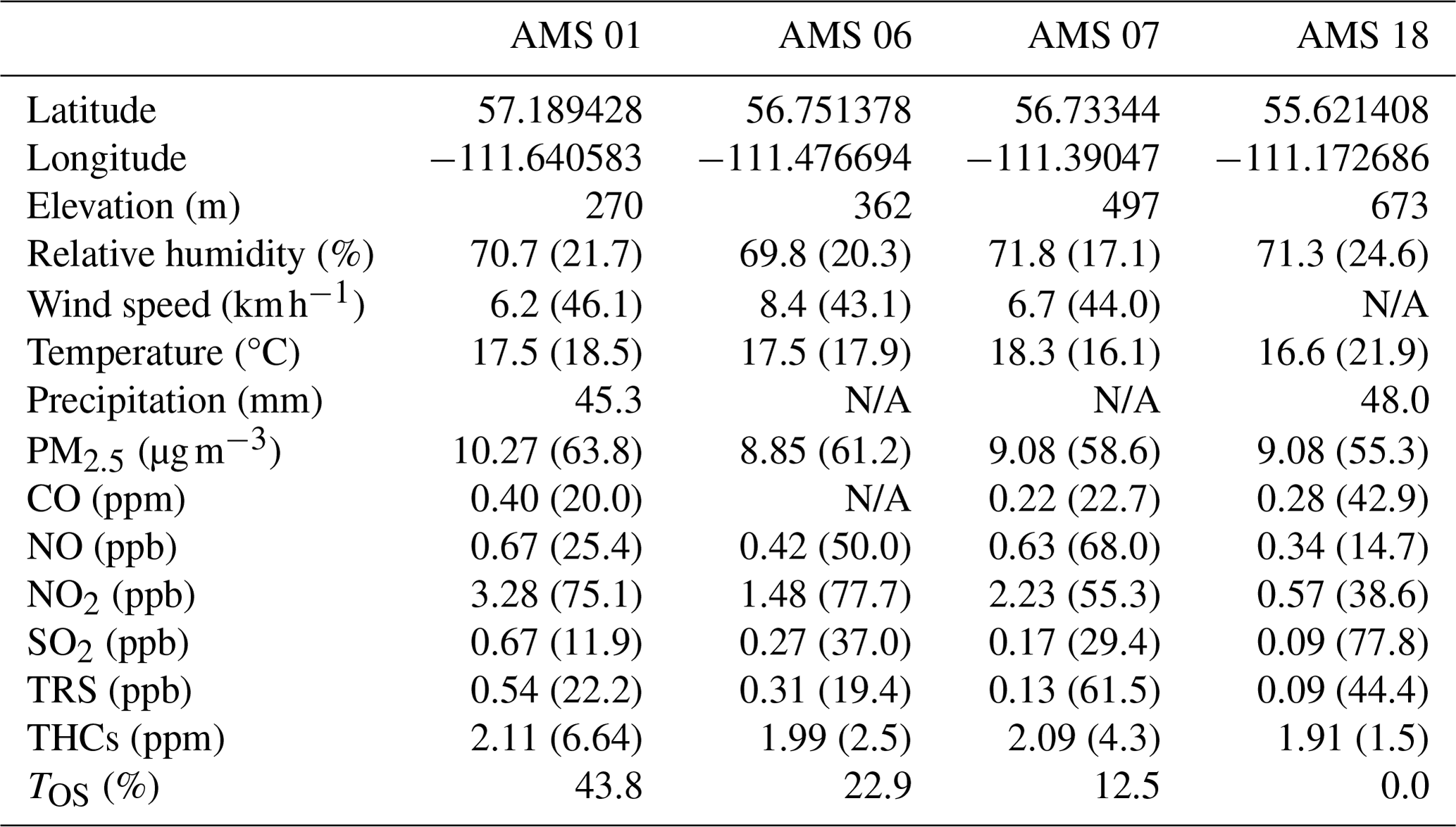
N/A: not available.

Evaluation of WBEA station PM_2.5 time series data identified two periods of elevated concentrations. The first and most intense event (with an hourly maximum PM_2.5 value > 140 µg m⁻³) occurred between 19 and 22 July, while the second event occurred from 31 July to 6 August (with an hourly maximum PM_2.5 value of ∼ 50 µg m⁻³) (Fig. S2). These high-PM_2.5 events occurred during relatively similar periods across the monitoring stations (including AMS 18), suggesting a shared regional source. Trajectory frequency analysis indicated that extensive wildfires in northern Saskatchewan were the primary source of smoke (PM_2.5) in the study region (Fig. S3).

The T_OS analysis demonstrated that the relative influence of OS emissions was strongest at the DP2050 (79.2 %) and AMS 01 (43.8 %) sites, followed in descending order by the AMS 06, AMS 07, and AMS 18 sites. Differences in our analysis at each of these sites can thus be used to infer source-related differences in composition (Table 1). Comparison of HYSPLIT trajectories against corresponding continuous station data showed general agreement between modelled and observed wind directions across the exposure periods (Fig. S4). Bivariate analysis demonstrated strong positive correlations (R_S = 0.83–0.92) between T_OS and continuous pollutant species reported by the WBEA (exposure-averaged NO, NO₂, SO₂, TRS, and THCs; Table A3), indicative of emission transport from OS facilities. Frequency estimates displayed weaker agreement with average PM_2.5 and CO values (R_S < 0.50), likely due to the influence of non-OS sources, namely wildfire smoke.

3.2 Active-sampler TSP summary

Throughout the study, the DP2050 sampler measured elevated concentrations of DIC, ${\mathrm{NO}}_{\mathrm{3}}^{-}$, ${\mathrm{SO}}_{\mathrm{4}}^{\mathrm{2}-}$, Na, P, S, V, Fe, and Sr compared to the other study sites, while most variables (with the exception of WSOC and TDN) were reduced at AMS 18 (Table 2). Measured WSOC and Abs₃₆₅ values were significantly higher at the near-field DP2050 site compared to the remaining stations (Kruskal–Wallis test; α < 0.05), while MAE₃₆₅ values were similar across all sampling locations (Kruskal–Wallis test; α > 0.05). Dissolved V, Sr, S, and Na were strongly (positively) correlated (R_S > 0.77) with T_OS estimates, while WSOC and Abs₃₆₅ displayed weak positive agreement (R_S ≥ 0.45; Table A4) with T_OS. Both WSOC and absorbance values were occasionally elevated during individual exposures (i.e. at AMS 18 from 5–7 August (WSOC = 7.2 µg C m⁻³; Abs₃₆₅ = 7.7 m⁻¹)), receiving limited industrial influence but high levels of wildfire atmospheric transport (Fig. S5), while MAE₃₆₅ displayed limited patterns in relation to wildfire smoke events. Moreover, WSOC and Abs₃₆₅ were moderately correlated according to Spearman's correlation test (R_S = 0.30; α < 0.05).

Table 2 Summary of the active-sample variables (with corresponding MDLs; ng m⁻³) measured during the study period (19 July–10 August) at each monitoring location. Median and normalized median absolute deviation values, with the latter presented in brackets and as percentages, are shown for each variable and site. Sampling locations are ordered according to latitude (N to S).

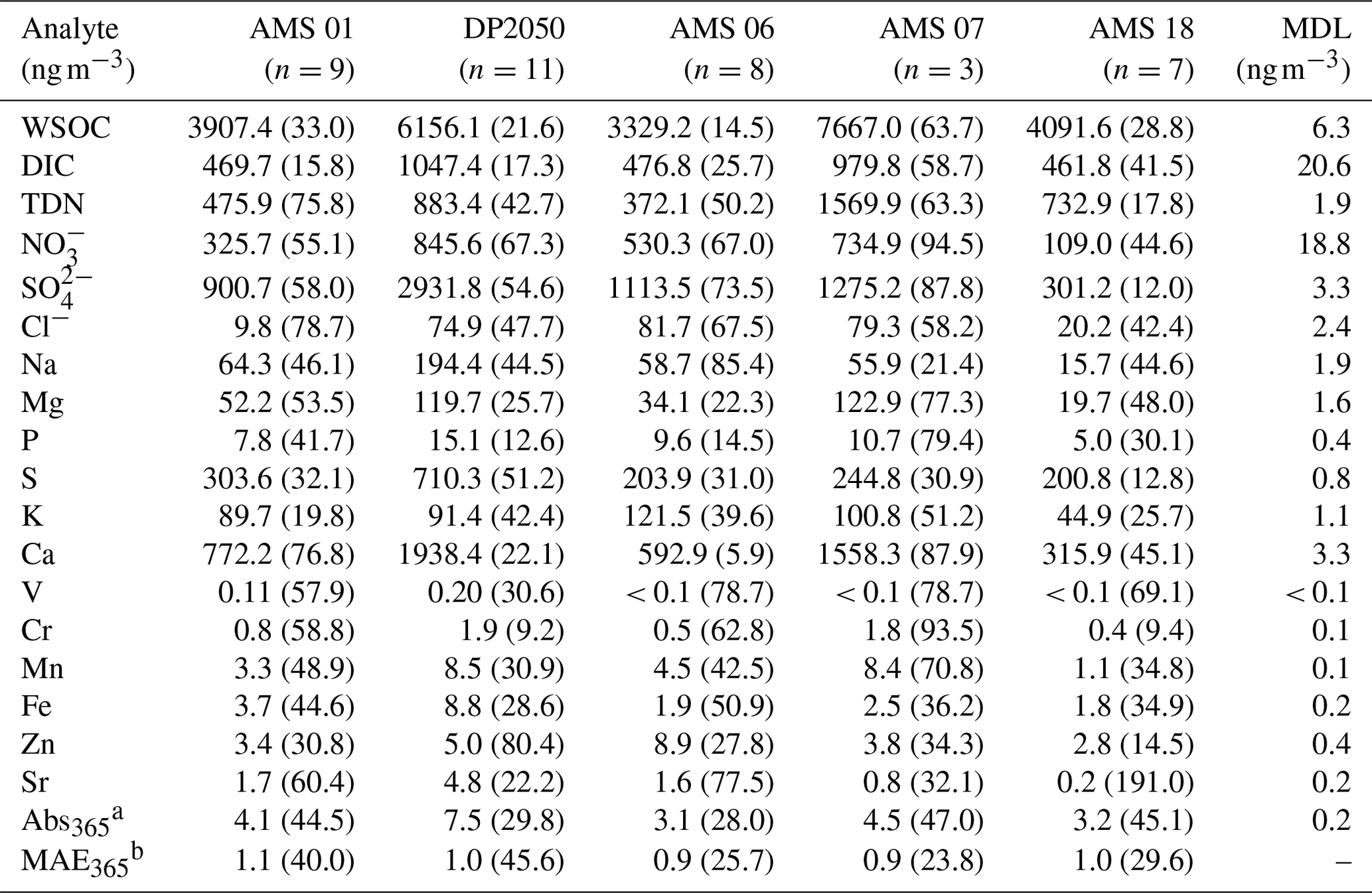
^a Reported in m⁻¹ (including the final column). ^b Reported in ${\mathrm{m}}^{-\mathrm{2}}\mathrm{g}{\mathrm{C}}^{-\mathrm{1}}$.

3.3 Fluorescence

The EEMs produced from the TSP samples frequently displayed peak fluorescence (> 30 QSU) within the λ_Ex and λ_Em wavelength ranges of 210–350 and 390–430 nm, respectively. Moreover, secondary peaks (> 20 QSU) were observed within the excitation range of 200–250 nm and the emission range of 250–400 nm. Fluorescent scans of raw bitumen and dry MFT materials produced strong peaks (> 30 QSU) in similar regions, with λ_Ex values of 200–250 nm and λ_Em values of 250–400 nm, and limited fluorescence within higher ranges (λ_Ex values of 210–350 nm and λ_Em values of 390–430 nm) (Fig. A1). Similar scans of unpaved road dust materials displayed fluorescence in the λ_Ex range of 200–250 nm and λ_Em range of 250–400 nm; however, emission intensity was weak (≤ 8 QSU).

Comparative analysis of multiple PARAFAC models indicated that a model rank of 3 was most appropriate – that is, the data suggested that three distinct classes of organic compounds were present. The three-component model displayed a high degree of fit (0.95), a CC of 96.2, and a split-half validation score of 0.87. The modelled components displayed clearly defined fluorescent peaks/regions, while no distinct or recurring residual peaks were observed within the model output (Fig. 2).

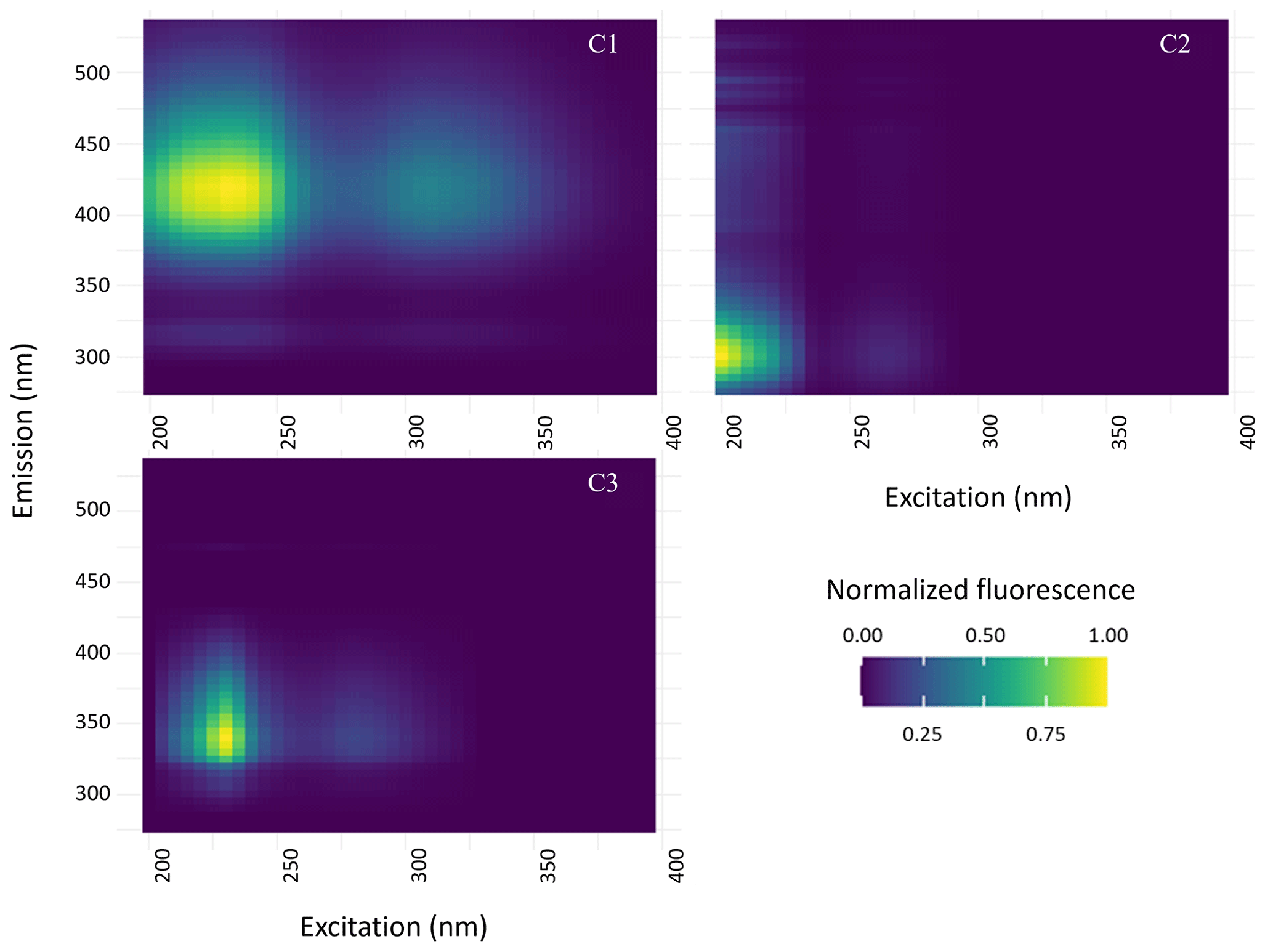
Figure 2 Visualization of the three PARAFAC components (C1–C3) generated from the combined TSP–EEM sample set. Emission intensity values are normalized to the maximum component fluorescence.

The first fluorescent component (C1) presented two emission peaks that are generally classified as atmospheric HULISs in the BrC literature (Dey and Sarkar, 2024; Laskin et al., 2015). Several water-quality studies have associated similar peaks with fluorophores of petrogenic or anthropogenic origin (Brünjes et al., 2022; Zito et al., 2019). The second component (C2) was reflective of PRLIS aerosols (Dey and Sarkar, 2024; Dong et al., 2024; Laskin et al., 2015), while the third component (C3) was identified as a BrC PRLIS with spectra similar to those of anthropogenic (Cao et al., 2023; Yan et al., 2020) and petrogenic (Whisenhant et al., 2022) fluorescent DOM.

Median F_MAX (normalized median absolute deviation) values for C1–C3 were 6.0, 34.6, and 10.4 QSU m⁻³ (100.0 %, 39.5 %, and 66.9 %), respectively, demonstrating that the C2 amino-acid-like component was the dominant fluorophore. The average RPD for the study, calculated from duplicate exposures, was 10.7 %, 8.5 %, and 9.6 % for C1–C3, respectively. Values of both F_MAX and WSOC-normalized fluorescence (C_WSOC) for C1 and C3 were highest at the near-field industrial sampling locations (DP2050, AMS 01), followed by the mid-field urban sites (AMS 06, AMS 07), while the lowest values were reported at the background location (AMS 18) (Fig. 3), indicating a greater likelihood of C1 and C3 having OS-related sources. Moreover, measured fluorescence at DP2050 and AMS 01 was significantly higher (Kruskal–Wallis test; α < 0.05) than at AMS 18, further indicating that OS operations were a dominant source of C1 and C3. The second fluorescent component (C2) displayed a distinct decrease in fluorescence intensity as a function of distance from OS operations. Although C2 PRLIS fluorescence was significantly elevated at DP2050 compared to all downfield sites (excluding AMS 07 due to its small sample size), a comparison of the remaining sampling locations (including AMS 18) revealed insignificant differences in the measured fluorophore intensity. The high relative fluorescence at the background station suggests that a broader regional (non-OS) source contributed to C2 in the study region.

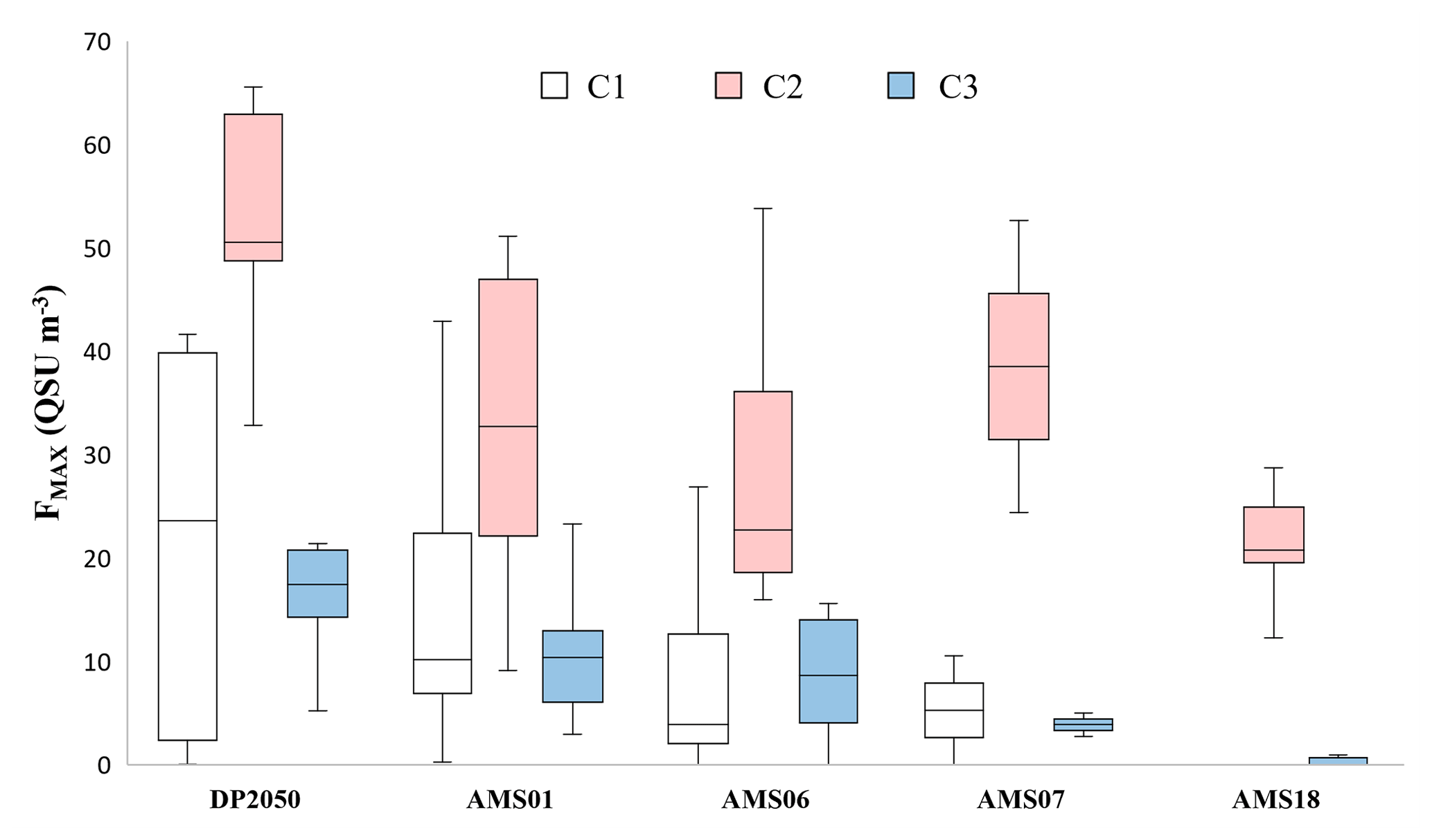
Figure 3 Distributions of component (C1–C3) fluorescence (QSU m⁻³) measured at each sampling location during the study period (19 July–10 August).

Both C1 and C3 displayed strong positive correlations (R_S = 0.77 and 0.88, respectively) with T_OS (Fig. 4; Table A3), suggesting that fluorescence was elevated when samplers received atmospheric transport from OS operations. As specific examples, two Mildred Lake exposures (6–8 and 8–10 August) with distinctly high C1 and C3 values (> 100 and > 38 QSU m⁻³, respectively) were associated with strong SW winds (≥ 10 km h⁻¹) that passed over adjacent tailing ponds (∼ 1 km from the site), open-pit mines, and active upgrading facilities (Fig. 5). High F_MAX exposures at AMS 06 between 4 and 6 August coincided with N–E winds passing over upwind facilities (Fig. A2). Conversely, when samplers received atmospheric transport from undeveloped and forested regions, C1 and C3 values were markedly lower (Fig. 5). Although generally elevated when downwind of OS facilities, C2 was occasionally heightened when sites received non-industry trajectories (Fig. S5). This inconsistency is reflected by the comparatively weaker correlation between T_OS and C2 fluorescence (R_S < 0.62). The WSOC-normalized fluorescence (C1_WSOC–C3_WSOC) displayed spatial trends relatively similar to those of C1–C3 (Fig. A3).

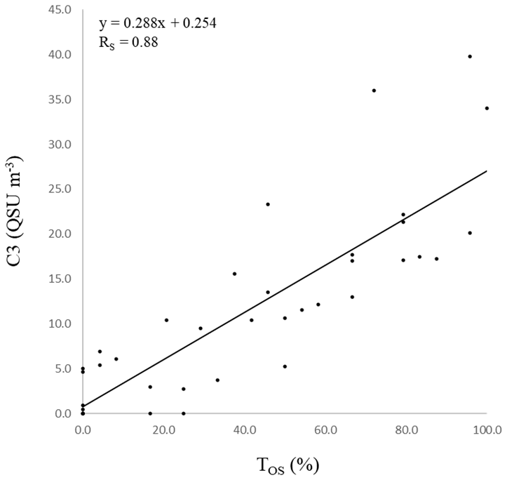
Figure 4 Bivariate comparison of active-sampler-measured C3 fluorescence (QSU m⁻³) and corresponding OS trajectory frequency (T_OS) estimates, expressed as percentages, over the study period. The line of best fit, along with the corresponding regression equation and Pearson correlation coefficient (R_S), is displayed.

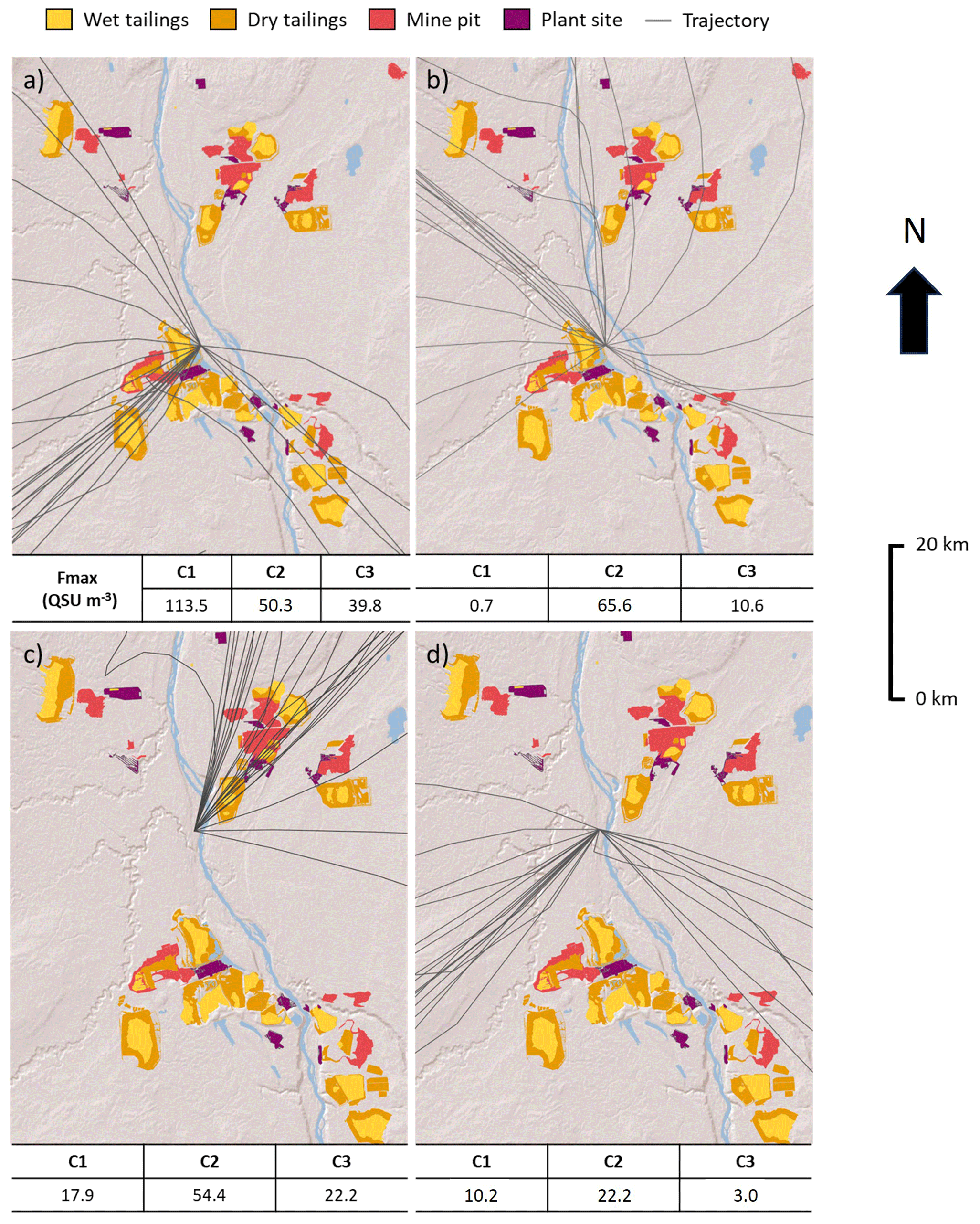
Figure 5 Spatial distributions of 48 h atmospheric back trajectories (black lines) converging at sampling locations during selected exposure periods. (a) DP2050 (6–8 August). (b) DP2050 (29–31 July). (c) AMS 01 (4–6 August). (d) AMS 01 (21–23 July). F_MAX values (QSU m⁻³) for C1–C3, measured during each exposure, are shown beneath the corresponding trajectory plots. The spatial boundaries of various OS facilities, including wet tailings (yellow), dry tailings (orange), open-pit mines (red), and plant sites (purple), are shown (ESRI 1995–2024).

The fluorescent components C1 and C3 varied independently of wildfire transport; for example, low C1 and C3 concentrations (< 0.5 and 5.2 QSU m⁻³, respectively) were recorded during the high-smoke event at DP2050 (19–20 July; Fig. S5), while some of the highest F_MAX values were recorded during relatively smoke-free exposures at the same site (8–10 August; C1 = 137.6 QSU m⁻³; C3 = 20.1 QSU m⁻³). In contrast, high C2 concentrations frequently occurred during wildfire events, where back trajectories displayed winds originating from fire-affected regions in British Columbia or Saskatchewan (Fig. S5).

3.4 Comparison of fluorophores against supplementary TSP variables

Comparison against continuous station data showed that C1 and C3 were positively correlated (Spearman's correlation test; α < 0.05), with most pollutant species (Table A3), while C2 displayed comparatively weaker correlations with continuous data. Evaluation of the complete TSP dataset showed that C1 was strongly (positively) correlated (R_S > 0.70) with ${\mathrm{NO}}_{\mathrm{3}}^{-}$, ${\mathrm{SO}}_{\mathrm{4}}^{\mathrm{2}-}$, Na, Mg, S, V, and Sr; C3 displayed similar trends, exhibiting additional correlations with Ca, P, and Mn. Moreover, C2 was moderately correlated with WSOC, DIC, Na, Mg, P, S, Ca, V, Cr, Mn, and Sr (Table A4).

Cross-validation confirmed that the two-component PLS-R model produced relatively high R²Y values (cumulative R²Y = 0.73) and the highest cumulative Q²Y value (0.57). The first modelled component (PLS1; R²Y = 0.49) was primarily defined (VIP score > 1) by ${\mathrm{NO}}_{\mathrm{3}}^{-}$, ${\mathrm{SO}}_{\mathrm{4}}^{\mathrm{2}-}$, Na, Mg, P, S, Ca, V, Mn, Sr, and T_OS, while the second component (PLS2; R²Y = 0.24) was characterized by WSOC, DIC, ${\mathrm{SO}}_{\mathrm{4}}^{\mathrm{2}-}$, Na, P, V, and T_OS. Of these variables, Na and T_OS were the most important (VIP score > 1.4) for both PLS1 and PLS2. Considering that certain OS fugitive emissions (e.g. tailing sand and haul road dust) are often Na-enriched (Wang et al., 2015), these high VIP scores suggest that both dimensions represent industrial sources. Moreover, PLS1 was positively correlated with variables previously linked to crustal (Mg, Ca, Mn) and bituminous (S, Sr, V) sources, which, in the case of the AOSR, could be reflective of bitumen and overburden excavation (Landis et al., 2012). Regarding PLS2, the positive correlation with Na, ${\mathrm{SO}}_{\mathrm{4}}^{\mathrm{2}-}$, and T_OS could represent non-crustal industrial sources (Wang et al., 2015), while the negative correlation with WSOC and DIC may reflect non-OS carbonaceous PM emissions. Biplot visualization revealed that C1 and C3 fluorescence were positively correlated with both PLS-R components and plotted near Na (Fig. 6); both fluorophores were notably distant from WSOC and Abs₃₆₅. The second fluorescent component displayed a strong positive correlation with the first PLS-R component and was plotted in proximity to WSOC, DIC, Ca, Mn, and Abs₃₆₅. A score plot visualization of individual exposures displayed a general separation between DP2050 and the remaining sites along the first PLS-R component axis (Fig. A4). The PLS-R models generated using WSOC-normalized component fluorescence (C1_WSOC–C3_WSOC) as Y variables were comparatively weak as the two-component model displayed low cumulative R₂Y and Q₂Y scores (0.48 and 0.18, respectively).

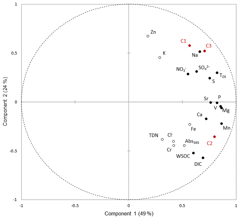
Figure 6 Correlation biplot displaying both X (black) and Y (red) variables in relation to the first two partial least-squares regression components. Filled and unfilled black circles represent X variables assigned high (≥ 1) and low (< 1) VIP scores, respectively.

4 Discussion

4.1 WSOC and WS-BrC absorption

Ambient WSOC levels in the AOSR (including at AMS 18) were higher than TSP-based (summertime) measurements (WSOC < 1 µg C m⁻³) from the remote southern Tibetan Plateau (Cong et al., 2015; Li et al., 2021) and Greenland ice sheet (Hagler et al., 2007) but similar to the magnitude of values (1–10 µg C m⁻³) reported from the city of Pune, India (Kirillova et al., 2013); Bangkok, Thailand (Tang et al., 2021); and Karachi, Pakistan (Chen et al., 2020), as well as that of values measured in peatland-fire-affected samples from western Russia (Popovicheva et al., 2019). Conversely, WSOC levels in the AOSR were generally lower than measured concentrations (> 10 µg C m⁻³) in New Delhi, India (Kirillova et al., 2014; Miyazaki et al., 2009).

Compared to previous studies focused on the TSP fraction, Abs₃₆₅ values in the AOSR were generally higher than summertime values reported from remote regions, including the Tibetan Plateau (Abs₃₆₅ = 0.4 m⁻¹; Zhu et al., 2018), Gobi Desert (1.9 m⁻¹; Wen et al., 2021), and Amazon Basin (< 1.4 m⁻¹; Saturno et al., 2018), similar to observations from Bangkok (4.5 m⁻¹; Tang et al., 2021), and lower relative to polluted urban areas in eastern China (8.4 m⁻¹; Wen et al., 2021). Observed MAE₃₆₅ values in the AOSR were 25 %–400 % higher than values reported across a variety of studies (Srinivas and Sarin, 2013; Tang et al., 2021; Wu et al., 2019), demonstrating that WS-BrC possessed a relatively high light absorption capacity.

The moderate positive correlation between WSOC and Abs₃₆₅ indicates that WS-BrC was an appreciable constituent of soluble organic carbon in the study region and that both TSP fractions likely shared select environmental sources. Higher WSOC and Abs₃₆₅ values at DP2050, relative to the other study sites, indicate that industrial operations may have contributed to regional WS-BrC values; the significant positive correlation between Abs₃₆₅ and T_OS further supports this assertion. However, the similarity between WSOC and Abs₃₆₅ among the remaining stations (excluding DP2050) implies that the extent of OS influence was spatially limited and that regional sources were the primary determinant of BrC at locations further afield. Elevated WSOC and absorbance during smoke events (e.g. at AMS 18 from 5–7 August) suggest that biomass combustion was a source of BrC. Regional wildfire smoke may explain why TSP-phase WSOC and Abs₃₆₅ at the background site (AMS 18) were higher than in other remote areas, such as the Tibetan Plateau and Greenland ice sheet (Hagler et al., 2007; Zhu et al., 2018), but comparable to WSOC concentrations observed during boreal fire events in western Russia (Popovicheva et al., 2019). Insignificant differences in MAE₃₆₅ between the AOSR sites, along with inconsistent MAE₃₆₅ values during extreme fire smoke events, demonstrate that aerosol light absorption capacity was not dependent upon OS or wildfire sources.

4.2 C1 and C3 fluorescent components

Elevated C1 and C3 fluorescence levels at near-field (< 5 km) industrial sites (DP2050, AMS 01), as well as significant positive correlations with T_OS and continuous pollutant data, indicate that OS emissions contributed to the measured fluorescence. Decreased F_MAX values during exposures where air masses originated from non-OS areas and/or background regions (i.e. AMS 01 (21–23 August) and AMS 18, respectively) further indicate that industrial operations were the primary source of C1 and C3 in the AOSR. Moreover, the low emission intensity (with the exception of C2) during smoke events (DP2050 (19–20 July) and AMS 18 (5–7 August); Fig. S5) demonstrates that biomass combustion was not the primary source of C1 and C3 fluorescence.

Source apportionment studies have identified bitumen excavation and hauling as key sources of PM in the AOSR, with emissions often associated with Na, S, and V (Landis et al., 2012, 2017). Therefore, the importance of Na and ${\mathrm{SO}}_{\mathrm{4}}^{\mathrm{2}-}$ as predictors of C1 and C3 variation could further link bitumen emissions to observed fluorescence. The spectral similarity between the raw-bitumen EEM and C3 PRLIS confirms that OS material likely contributed to at least one of the observed fluorescent peaks. Resuspended OS materials have been shown to significantly contribute to atmospheric loadings of total PAC species (Landis et al., 2019), where somewhat water-soluble, low-molecular-weight (LMW) PACs (i.e. naphthalene, fluorene, and dibenzothiophene) can fluoresce within the excitation and emission wavelength ranges, as observed for C1 (Driskill et al., 2018). Photodegradation of exposed bituminous material can produce oxygenated PACs (Yang et al., 2016), which, due to their enhanced water solubility, may additionally contribute to WS-BrC fluorescence.

Fugitive dust emissions from tailing ponds are an additional source of PM in the study region (Landis et al., 2012, 2019; Zhang et al., 2016). Due to the application of NaOH in accelerating the crude extraction process (Bakhtiari et al., 2015), OS tailings contain high concentrations of Na (MacKinnon and Sethi, 1993; Wang et al., 2015). The strong association of Na with C1 and C3 (via PLS-R) provides evidence suggesting that tailing dust contributed to the observed fluorescence. Oil sands tailing dust has been identified as a source of one- to three-ring PACs and naphthenic acids (Landis et al., 2012; Yassine and Dabek-Zlotorzynska, 2017; Zhang et al., 2016), which can fluoresce in λ_Ex and λ_Em regions, as observed for C1 and C3 (Driskill et al., 2018; Kaur et al., 2014). The spectral similarity between C3 and MFT reference material, along with elevated C1 and C3 emission intensities during exposures downwind of the tailing sites, further suggests that fugitive facility emissions contributed to BrC fluorescence.

Emission source profiles previously identified in the AOSR have been shown to contain loadings indicative of both crustal (Mg, Ca, Mn) and petrogenic (S, V, Ni) origins (Landis et al., 2012), largely due to the proximity and co-emission of different dust sources associated with OS activities. The first PLS-R component, which displayed strong correlations with Mg, Ca, Mn, C1, and C3, may be broadly representative of crustal emissions (e.g. haul road dust, excavated surface soils, and overburden) from OS operations. However, the separation of Mg, Ca, and Mn from C1 and C3 along the second PLS-R component (i.e. non-crustal) axis plot implies that the fluorophores were co-emitted alongside these crustal sources.

Analysis of the current TSP dataset was unsuccessful in distinguishing between C1 and C3, likely indicating the co-emission of these fluorophores from industrial sources. However, unlike C3, the C1 HULIS fluorophore did not match the EEM spectra produced from the raw bitumen or MFT extracts, suggesting that the two fluorophores originated from different emission sources associated with OS operations. Industrial facilities in the AOSR often contain stockpiles and beaches comprised of petroleum coke (petcoke), a carbon-rich derivative of the oil-refining process that has been identified as a major source of particulate PAC emissions in the surrounding region (Zhang et al., 2016). Fugitive petcoke dust co-emitted from OS facilities may have contributed to the observed C1 fluorescence. Future BrC field studies should consider increasing the number of sampling locations near a diverse range of OS facilities, shortening exposure periods to limit source mixing, and expanding the analysis of complementary OS indicator variables (e.g. molybdenum, nickel, and PACs; Landis et al., 2019) to better characterize C1 and C3 source profiles in the AOSR.

4.3 C2 fluorescent component

Significant positive correlations between C2, WSOC, and Abs₃₆₅ suggest that the fluorophore was a key constituent of bulk WS-BrC in the AOSR, consistent with the observed dominance of C2 over the total sample fluorescence. Significantly elevated C2 values at the near-field (< 1 km) Mildred Lake site, along with comparable fluorescence at AMS 18 relative to the remaining stations, suggest that both industrial and broad regional sources contributed to BrC across the study area, consistent with what was observed for WSOC and Abs₃₆₅.

Occasionally elevated fluorescence during regional smoke events (e.g. at DP2050 from 19–20 July) indicates that wildfire smoke contributed to C2 fluorescence; this is unsurprising given that biomass combustion is one of the leading sources of BrC globally (Chen and Bond, 2010). Particulate matter originating from biomass combustion can contain substantial amounts of water-soluble organic carbon (Park et al., 2013; Pastor et al., 2020), which may explain the observed association between WSOC and C2. Future evaluations of BrC in the AOSR should also measure pyrogenic tracer species, such as retene and levoglucosan, as these organic compounds can be used for wildfire source apportionment (Wentworth et al., 2018).

The similarity in fluorescent spectra when comparing C2 and road dust EEMs indicates the potential influence of crustal fugitive dust emissions on fluorescent PM. Haul roads throughout the AOSR are generally constructed using locally excavated limestone and bitumen, and regional road dust emission profiles often contain high loadings of DIC, Mg, Ca, and Mn (Wang et al., 2015). The observed association (PLS-R) between these variables and C2 among the TSP samples further supports the potential influence of road dust emissions on measured fluorescence. Road dust materials can contain a variety of chromophoric organic matter, including amino acids (Chalbot and Kavouras, 2019) and LMW PACs (as in the case of haul and industrial roads in the OS) (Landis et al., 2019), which can fluoresce in low λ_Ex and λ_Em wavelength ranges, as observed for C2 (Christensen et al., 2005; Kim and Koh, 2020). Following initial suspension, larger-diameter road dust particles are rapidly removed from the atmosphere through physical interactions with the surface environment (vegetation, human-made structures, etc.). For example, Veranth et al. (2003) found that irregular surface conditions adjacent to an unpaved road in Utah (United States) contributed to an 85 % reduction in coarse particulate matter within 100 m of the emission source. In the case of the AOSR, industrial haul roads close to (< 1 km from) site DP2050 contributed to elevated C2 fluorescence, while rapid removal further downwind possibly explains why C2 values were relatively similar between the remaining downfield sites. In the absence of an appreciable influence of OS road dust, regional wildfire smoke likely became the dominant source of C2 fluorescence. Future studies should consider using pyrogenic (retene, levoglucosan) and petrogenic (molybdenum, nickel, PAC) indicator variables to determine the relative contributions of wildfire and OS emission sources to C2 fluorescence in the AOSR.

5 Conclusions

Optical analysis of atmospheric TSP samples collected throughout the AOSR showed that OS activities were a measurable source of WS-BrC in the surrounding airshed during the summer season. Significantly higher Abs₃₆₅ values measured at the industry-adjacent site (DP2050) demonstrated that OS operations likely enhanced aerosol light absorbance, which, in turn, may have impacted local solar-radiation budgets and atmospheric photochemistry. However, statistically similar Abs₃₆₅ and MAE₃₆₅ values across the remaining stations indicated that the influence of OS emissions on WS-BrC absorbance was spatially limited and unlikely to substantially influence the regional climate during the summer. Combined EEM–PARAFAC evaluation of the TSP samples identified three distinct fluorophores (C1–C3), all of which exhibited a potential link to industrial activity. However, uniformly elevated C2 emission intensity during wildfire smoke episodes indicated that biomass combustion was also a considerable source of PRLIS aerosols in the region, while C1 and C3 were predominantly linked to OS sources.

As far as the authors are aware, this is the first study to evaluate WS-BrC in the AOSR airshed. Considering the low operational costs compared to those of conventional methods of mass spectrometry, UV–Vis spectroscopy and the EEM–PARAFAC method offer accessible techniques for monitoring WS-BrC and initially screening for OS-sourced aerosols throughout the AOSR. Moreover, the capacity of the EEM–PARAFAC method to identify fluorescent species strongly linked to industry suggests that similar spectroscopic techniques could be employed to evaluate WS-BrC near other oil and gas facilities worldwide.

Appendix A

Datasets were acquired using an Agilent 8800 triple-quadrupole inductively coupled plasma mass spectrometer at Trent University's Water Quality Centre. A MicroMist nebulizer (with a nominal uptake rate of 400 µL min⁻¹) and a Scott double-pass spray chamber were used for sample introduction.

Table A1 Instrument operating conditions and measurement parameters.

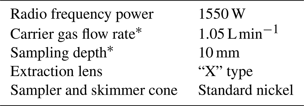
^∗ General purpose plasma preset.

Calibration standards were prepared using serial dilution of a 100 ng mL⁻¹ multi-element solution (HPS QCS 27) and 1000 ng mL⁻¹ single-element standards in 2 % HNO₃. High-purity water (18.2 MΩ cm) and nitric acid were used for the preparation of all solutions. The National Institute of Standards and Technology (NIST) Standard Reference Material (SRM) 1640a (“Trace Elements in Natural Water”), the National Research Council Canada (NRC) SLRS-6 (“River Water Certified Reference Material for Trace Metals and other Constituents”) reference material, and Canadian Association for Laboratory Accreditation proficiency testing (CALA PT) standards were used for QA/QC. The measured concentrations were within 5 % of the certified values.

Table A2 Instrument tune mode and scan type used to measure each element. MS/MS: tandem mass spectrometry.

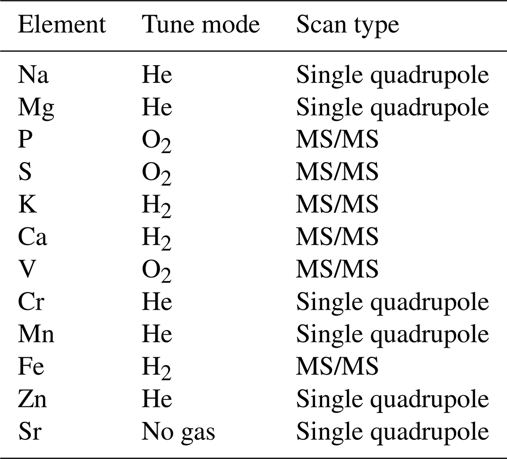
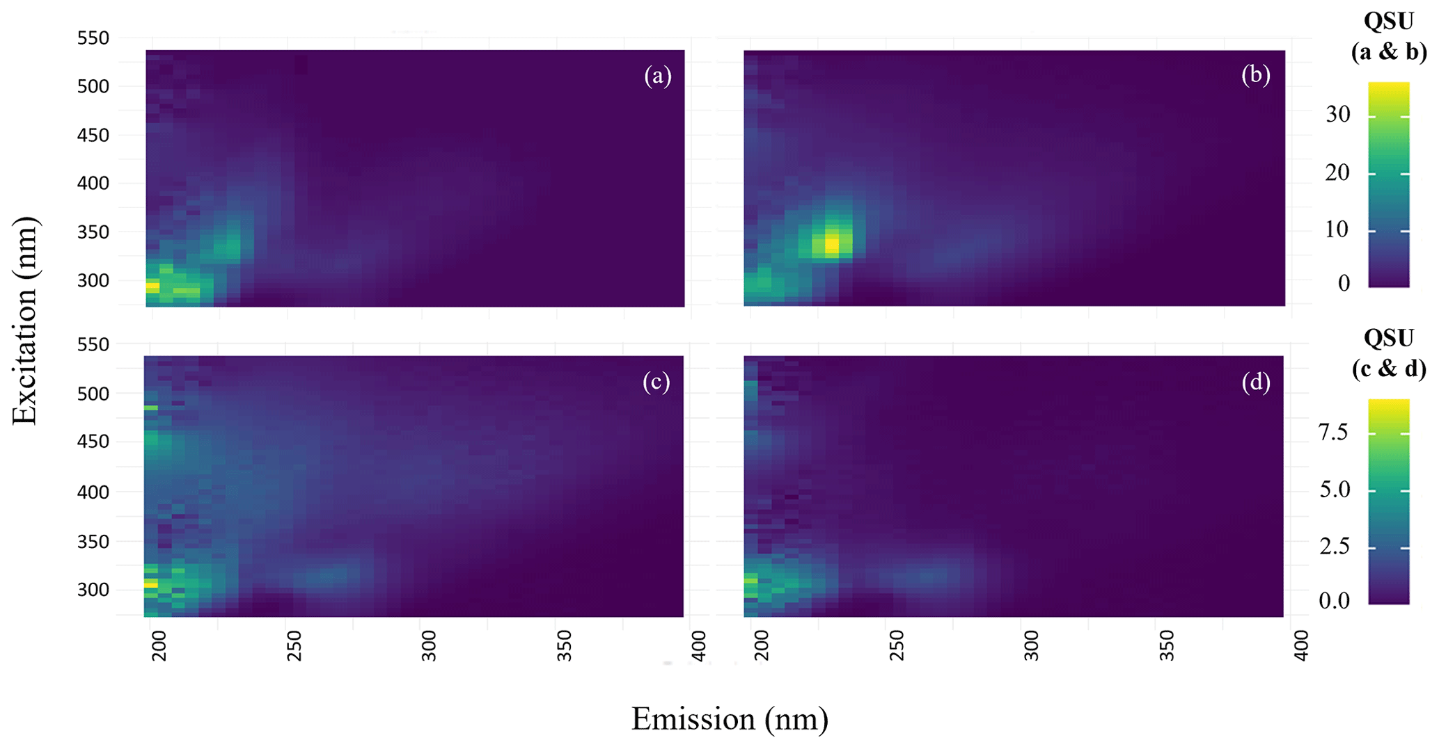
Figure A1 Visualization of the EEM scans produced from (a) raw bitumen, (b) dry MFTs, and unpaved road dust from (c) DP2050 and (d) AMS 01. Fluorescence intensity is displayed in quinine sulfate units (QSU). Note that panels (a) and (b) follow a different colour scale than panels (c) and (d).

Table A3 Spearman correlation analysis comparing absorbance indices (Abs₃₆₅, MAE₃₆₅), the modelled fluorescent components (C1–C3), the trajectory frequency (T_OS), and continuous pollutant species measured at the active-sampling locations (excluding DP2050). The correlation coefficient (R_S) for each significant correlation (α < 0.05) is shown.

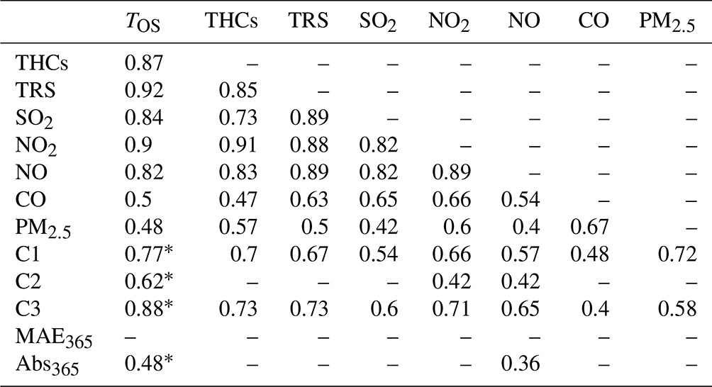
^∗ Correlation calculated using data from all stations, including DP2050.

Table A4 Spearman correlation analysis of the modelled fluorescent components (C1–C3) against corresponding chemical and optical variables measured through the active-sampler network. The coefficient (R_S) of each significant correlation (α < 0.05) is shown.

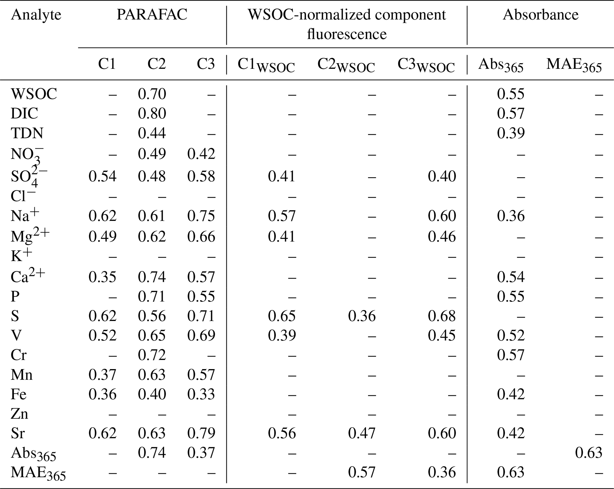
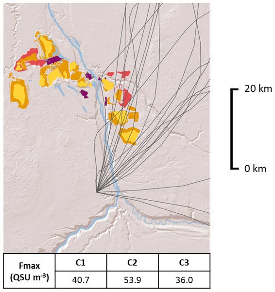
Figure A2 Spatial distributions of 48 h atmospheric back trajectories (black lines) converging at AMS 06 during the 4–6 August exposure. F_MAX values (QSU m⁻³) for C1–C3, measured during the corresponding exposures, are shown. The spatial boundaries of various OS facilities, including wet tailings (yellow), dry tailings (orange), open-pit mines (red), and plant sites (purple), are shown (ESRI 1995–2024).

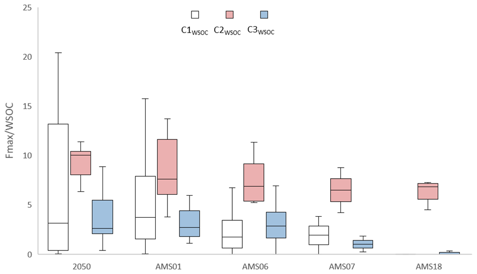
Figure A3 Distributions of WSOC-normalized component fluorescence (C1_WSOC–C3_WSOC) measured at each sampling location during the study period (19 July–10 August 2021).

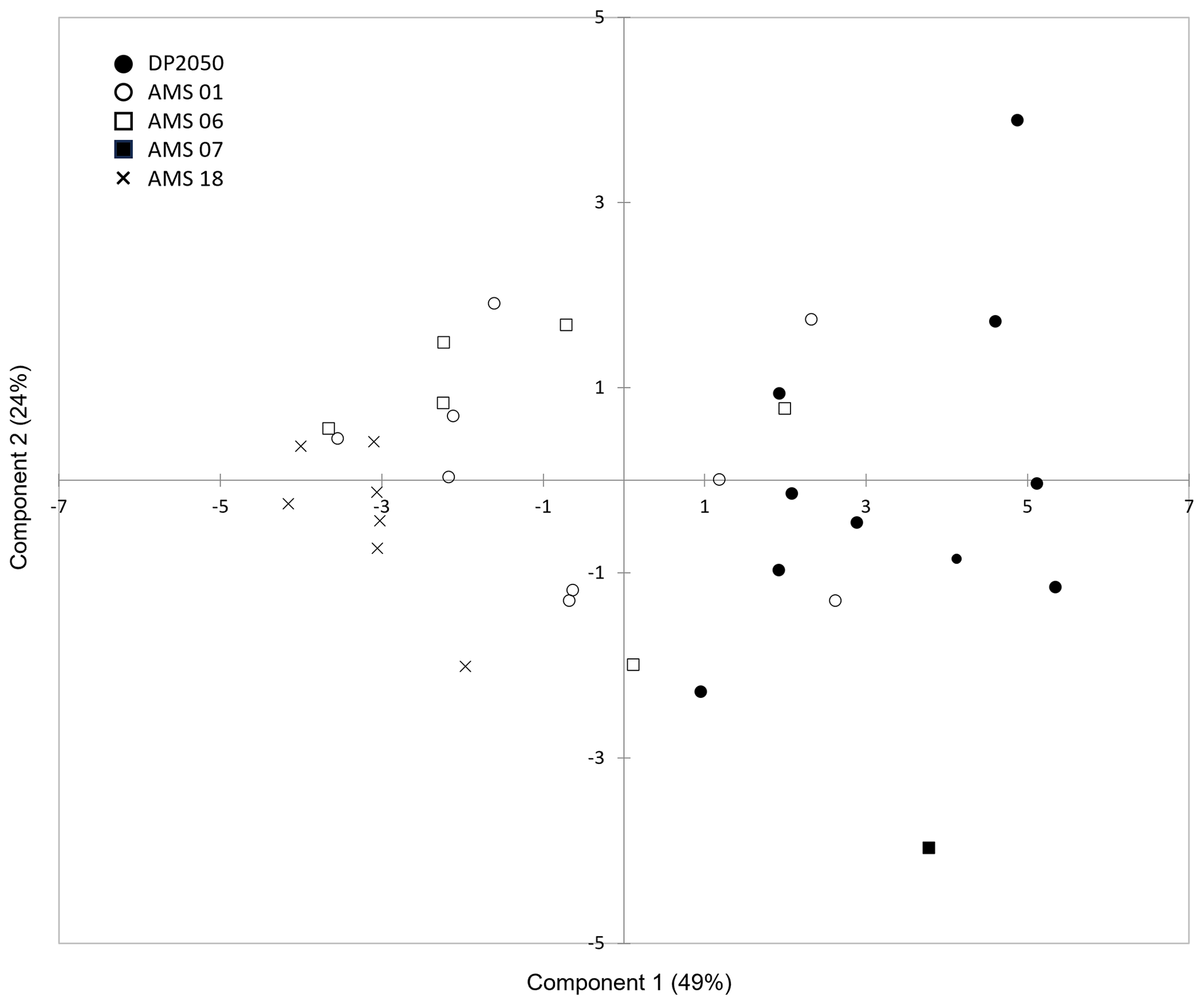
Figure A4 PLS-R biplot displaying distributions of observations relative to the first two modelled components. Observations are categorized by site ID: AMS 01 (unfilled circles), DP2050 (filled circles), AMS 06 (unfilled squares), AMS 07 (filled squares), and AMS 18 (crosses).