Impact of SO₂ injection profiles on simulated volcanic forcing for the 2009 Sarychev eruptions – investigating the importance of using high-vertical-resolution methods when compiling SO₂ data

Aerosols from volcanic eruptions impact our climate by influencing the Earth's radiative balance. The degree of their climate impact is determined by the location and injection altitude of the volcanic SO₂. To investigate the importance of utilizing correct injection altitudes, we ran climate simulations of the June 2009 Sarychev eruptions with three SO₂ datasets in the Community Earth System Model version 2 (CESM2), Whole Atmosphere Community Climate Model Version 6 (WACCM6). We have compared simulations with WACCM6 default 1 km vertically resolved dataset M16 with our two 200 m vertically resolved datasets, S21-3D and S21-1D. S21-3D is distributed over a large area (30 latitudes and 120 longitudes), whereas S21-1D releases all SO₂ in one latitude and longitude grid box, mimicking the default dataset M16.

For S21-1D and S21-3D, 95 % of the SO₂ was injected into the stratosphere, whereas M16 injected only 75 % into the stratosphere. This difference is due to the different vertical distributions and resolutions of SO₂ in the datasets. The larger portion of SO₂ injected into the stratosphere for the S21 datasets leads to more than twice as high sulfate aerosol load in the stratosphere for the S21-3D simulation compared to the M16 simulation during more than 8 months. The temporal evolution in aerosol optical depth (AOD) from our two simulations, S21-3D and S21-1D, follows the observations from the spaceborne lidar instrument CALIOP (Cloud-Aerosol Lidar with Orthogonal Polarization) closely, while the AOD in the M16 simulation is substantially lower. This indicates that the injection altitude and vertical resolution of the injected volcanic SO₂ substantially impact the model's ability to correctly simulate the climate impact from volcanic eruptions.

The S21-3D dataset with its high vertical and horizontal resolution resulted in global volcanic forcing of −0.24 W m⁻² during the first year after the eruptions, compared with only −0.11 W m⁻² for M16. Hence, our study highlights the importance of the vertical distribution of SO₂ injections in simulations of volcanic climate impact and calls for a re-evaluation of further volcanic eruptions.

1 Introduction

Aerosols impact our climate by influencing the Earth's radiative balance – directly by scattering and absorbing solar radiation and indirectly via influencing cloud properties. These effects result in a net cooling effect on the climate. Aerosol emissions from fossil fuel combustion have counteracted some of the warming effects of anthropogenic greenhouse gases (Hansen et al., 2023). However, aerosols' climate impact is still a subject of great uncertainty (IPCC, 2021). It is important to understand natural sources of aerosols in order to better understand how humans affect the climate via emissions of greenhouse gases (Myhre et al., 2013; Robock, 2000).

Explosive volcanic eruptions that inject effluents into the stratosphere are a natural source of the particle-forming gas SO₂ and can have a large impact on the climate (Robock, 2000). Volcanic SO₂ is converted into sulfuric-acid-forming particulate matter, which can remain in the stratosphere for months or years, inducing long-term negative radiative forcing by scattering incoming solar radiation (Sigl et al., 2015). The aerosol is eventually removed from the stratosphere in the extratropics when the air is transported to the troposphere (Sigl et al., 2015; Gettelman et al., 2011; Appenzeller et al., 1996; Solomon et al., 2011). The severity of the climate impact is determined by the explosivity of the eruption, the mass of the stratospherically injected SO₂, the injection altitude, and the location of the volcano (Robock, 2000; Kremser et al., 2016).

Volcanic eruptions have, from time to time, substantially cooled the Earth's climate (Sigl et al., 2015). The 1991 Mt. Pinatubo eruption is the most recent eruption when a large amount of SO₂ reached high up into the atmosphere and lowered the globally averaged surface temperature by several 10ths of a degree Celsius (Kremser et al., 2016). Apart from such large eruptions, less explosive eruptions have added to variability in the stratospheric aerosol load and have had a substantial effect on the climate (Andersson et al., 2015; Vernier et al., 2011; Friberg et al., 2018), including the Sarychev eruptions in June 2009, which are simulated in the present study.

The vertical distribution of SO₂ from a volcanic eruption is crucial information, since the altitude determines the residence time of the aerosols (Andersson et al., 2015; Friberg et al., 2018; Kremser et al., 2016; Robock, 2000). Aerosols in the stratosphere can have a residence time of several years, whereas tropospheric aerosols have a residence time of weeks or less (Kremser et al., 2016). Stratospheric aerosols thus have a prolonged climate impact compared to tropospheric aerosols (Robock, 2000; Deshler, 2008). For a volcanic eruption to affect the climate in the longer term, the emitted sulfur needs to reach the stratosphere, i.e., be an explosive volcanic eruption. Less explosive eruptions often position the SO₂ in the vicinity of the tropopause. To estimate the climate impact of such eruptions, it is of particular importance to place the SO₂ at the correct altitude (Schmidt et al., 2018).

To investigate volcanic eruptions and their climate impact, global Earth system models (ESMs) can be utilized. Global modelers often use satellite-based observations of volcanic SO₂ as input when simulating the volcanic impact on the stratosphere and climate. SO₂ satellite instruments are passive sensors and therefore lack direct vertical measurements. The altitudes of the SO₂ clouds are therefore indirectly estimated, resulting in coarse vertical resolution with substantial uncertainties. Clarisse et al. (2014) showed that IASI can provide SO₂ data with vertical resolution down to ∼ 2 km, and MIPAS has a vertical resolution of 3–5 km (Höpfner et al., 2015). This is 1 order of magnitude coarser than typical SO₂ layers from the June 2009 Sarychev eruptions (Sandvik et al., 2021). In Sandvik et al. (2021) we combined passive satellite measurements from the AIRS (Atmospheric Infrared Sounder) satellite instrument with the active satellite sensor CALIOP (Cloud-Aerosol Lidar with Orthogonal Polarization) and created an SO₂ inventory with approximately 60 m vertical resolution. With this method we create a 3D dataset where we provide altitude information for different SO₂ layers from the same eruption emitted at different times and altitudes.

ESM simulations of explosive volcanic eruptions' climate impact are generally run with vertical SO₂ profiles released above, or in the vicinity of, the volcano site (Timmreck et al., 2018). This requires that the meteorology and tropopause height are simulated correctly in order to represent the transport of the volcanic aerosol during the first few days after the eruption. Small errors in horizontal or vertical transport may cause errors in the evolution of the SO₂ distribution (Tilmes et al., 2023) and transport of the formed sulfate particles and ultimately in the resulting climate impact. Using a 3D dataset retrieved a few days after the eruption could reduce such uncertainties.

To investigate the importance of utilizing a highly vertically and horizontally resolved volcanic SO₂ emission dataset, we used the SO₂ dataset of Sandvik et al. (2021) as input to an ESM. We have modeled the eruptions of Sarychev Peak in June 2009. This volcano is located in the Northern Hemisphere (NH) at the center of the Kuril Islands (48.092° N, 153.20° E). This case is considered to be a complex series of volcanic eruptions since the volcano erupted for several days and injected SO₂ over a wide range of altitudes. The duration of the eruption was from 11 to 16 June, spreading SO₂ from 11–19 km altitude. The total mass of SO₂ emitted from the eruptions has been reported to range from 0.6 to 1.2 Tg (Carboni et al., 2016; Haywood et al., 2010).

In this study, we ran three simulations with different SO₂ emission datasets with the Community Earth System Model version 2 (CESM2.1), Whole Atmosphere Community Climate Model (WACCM). The first is WACCM's default volcanic SO₂ single-column dataset with an assumed vertical profile, at 1 km resolution (Mills et al., 2016). The second is a dataset at 200 m vertical resolution where the SO₂ is distributed over a wide geographical region representing the initial spread of SO₂ based on Sandvik et al. (2021). The third dataset is a hybrid between the first two and constitutes a single-column dataset at 200 m vertical resolution compiled from Sandvik et al. (2021). All simulations are evaluated by comparison to aerosol observations from the satellite sensor CALIOP.

2 Method

In this section, we describe the SO₂ datasets used in the Earth system model, how they were created, and the differences between them. A brief model description and a description of the satellite dataset we compare the model simulations to are also included in this section.

2.1 SO₂ data

We have inserted the SO₂ dataset of the 2009 Sarychev Peak eruption described in Sandvik et al. (2021). It was compiled by combining horizontally resolved SO₂ data from the Atmospheric Infrared Sounder (AIRS) satellite instrument aboard the satellite Aqua, with the vertical aerosol profiles from the CALIOP satellite instrument. The SO₂ and aerosol observed from these instruments were assumed to be co-located and therefore have the same height profile. The aerosol data from CALIOP (at 60 m resolution) were coupled to the SO₂ data from AIRS using the dispersion model FLEXPART (FLEXible PARTicle dispersion model), enabling retrieval of vertical profiles of the SO₂ layers with a high resolution (Sandvik et al., 2021). For a more detailed description of the method used to obtain this dataset, we refer the reader to Sandvik et al. (2021).

The Sarychev Peak erupted multiple times over several days, starting on 11 June and continuing for 5 d. However, most of the SO₂ was emitted on 15 June (Rybin et al., 2011). The dataset from Sandvik et al. (2021) contains data from AIRS swaths around midnight UTC between 18 and 19 June. The Sandvik et al. (2021) 3D dataset has a vertical resolution of 1 K in potential temperature, corresponding to 61 ± 56 m or 1.8 ± 2.9 mbar. In this study, we ran the model with a re-gridded version of this dataset with a vertical resolution of 200 m and a horizontal resolution of 0.95° latitude × 1.25° longitude.

Table 1 Properties of the three input SO₂ datasets.

2.2 Model description

Simulations were run with the “specified dynamics” (SD) version of WACCM6 (WACCM6-SD; Gettelman et al., 2019). WACCM6 is an extension of the Community Atmosphere Model version 6 (CAM6), and part of the Community Earth System Model version 2 (CESM2.1) (Danabasoglu et al., 2020). WACCM6 is a global high-top atmospheric model, spanning the surface to the thermosphere. WACCM6-SD has a top altitude of 140 km and 88 levels. We ran the model with a horizontal resolution of 0.95° latitude × 1.25° longitude with active atmosphere and land components but prescribed sea-surface temperatures (SSTs) and sea-ice concentrations (Gettelman et al., 2019).

WACCM6 includes advanced atmospheric chemistry in the troposphere, stratosphere, mesosphere, and lower thermosphere (TSMLT). The chemistry includes 231 solution species and the following chemical reactions: 150 photolysis reactions, 403 gas-phase reactions, 13 tropospheric heterogeneous reactions, and 17 stratospheric heterogeneous reactions. For the stratospheric reactions, three types of aerosol particles are included: sulfate, nitric acid trihydrate, and water–ice (Gettelman et al., 2019). Sulfates in the stratosphere are produced by the chemical oxidation of SO₂ by the OH radical. The sulfate will then, via intermediate steps, produce H₂SO₄ gas (Liu et al., 2012; Mills et al., 2017). The H₂SO₄ gas can either condensate on existing particles or form new particles through binary H₂SO₄–H₂O nucleation (Vehkamäki et al., 2002, 2013). The newly formed particles are added to the Aitken mode after growth according to the parameterization from Kerminen and Kulmala (2002).

Figure 1 (a) Vertical SO₂ profiles for the three input datasets of each simulation. The vertical profile for M16 and S21-1D is the summed total injection for the eruption on 15 and 16 June, whereas the vertical profile for S21-3D is the total injection on 19 June. (b) Vertically integrated total amount of SO₂ for the S21-3D dataset. The red triangle marks the location of the Sarychev Peak volcano. (c) Latitudinally integrated total amount of SO₂ for the S21-3D input dataset. (d) Longitudinally integrated total amount of SO₂ for the S21-3D input dataset.

WACCM6 utilizes the Modal Aerosol Module, four-mode version (MAM4), as standard. This includes Aitken, accumulation, coarse, and primary carbon mode (Liu et al., 2016). MAM4 in WACCM6 includes modifications of the aerosol code to better represent aerosol processes in the stratosphere (Mills et al., 2016). The MAM4 gas–aerosol exchange module treats stratospheric sulfate as aqueous SO${}_{\mathrm{4}}^{=}$. The H₂SO₄ equilibrium vapor pressure treats condensation and evaporation of H₂SO₄ in the stratosphere to allow for shrinkage and growth between the accumulation and coarse mode (Mills et al., 2016).

WACCM6-SD allows the simulations to be nudged. We have nudged with Modern-Era Retrospective analysis for Research and Applications, version 2 (MERRA-2), from the surface to 50 km with a relaxation between 50 and 60 km and no nudging above 60 km. The horizontal winds and surface pressure were nudged, while temperature nudging was not used.

2.3 Simulation description

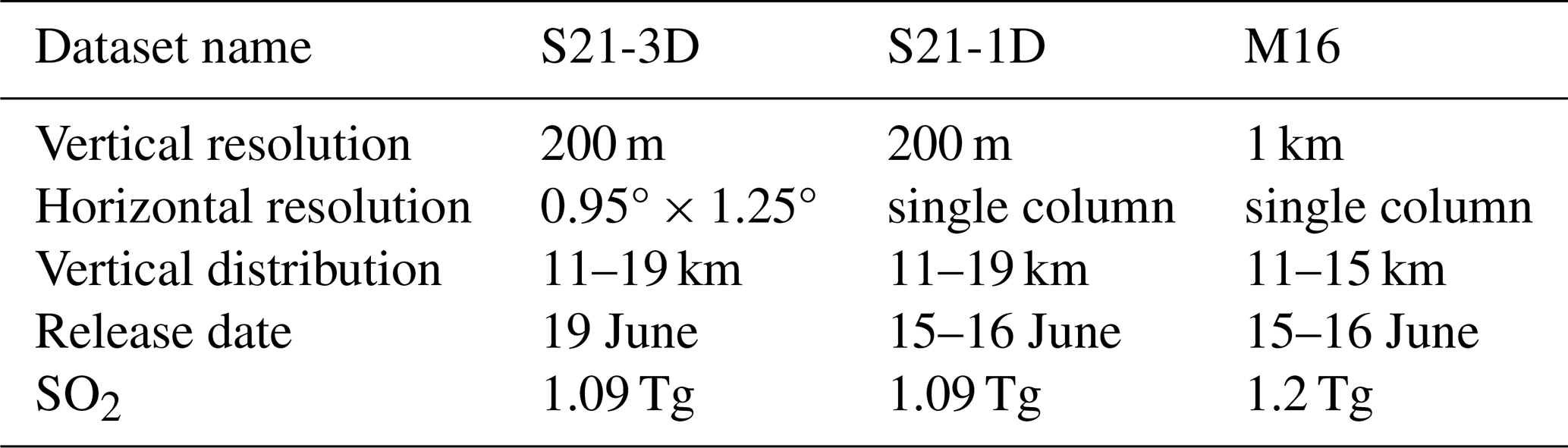
Three different simulations, referred to as S21-3D, S21-1D, and M16, were run over the period of January 2009 to December 2010 to investigate the eruption of Sarychev Peak in 2009, with different vertical and horizontal resolutions of SO₂ datasets as input. The differences between the input datasets for the simulations are summed up in Table 1, with further details below.

The first simulation, M16, was run with the default SO₂ dataset, Volcanic Emissions for Earth System Models, version 3.11 (VolcanEESM; Neely and Schmidt, 2016), for the Sarychev eruption from WACCM6. For 2009 and 2010, all eruptions except Sarychev's were removed. M16 is a single-column (1D) emission dataset with a vertical resolution of 1 km; 0.6 Tg of SO₂ was released on two occasions, 15 and 16 June, i.e., a total of 1.2 Tg. The SO₂ was released over a time period of 6 h, starting at 12:00 UTC and ending at 18:00 UTC. This is the same approach as that which has been used in previous studies of this eruption using WACCM (Neely and Schmidt, 2016; Mills et al., 2016).

The second simulation, S21-3D, was run with a volcanic SO₂ dataset for the Sarychev eruption and was created from the work of Sandvik et al. (2021). This dataset has a vertical resolution of 200 m and a horizontal resolution of 0.95° latitude × 1.25° longitude. The SO₂ is vertically distributed between 10 and 19 km and horizontally between the longitudes 130° E and 130° W (Fig. 1). The S21-3D dataset releases all 1.09 Tg of SO₂ over a time period of 2 h, starting on 19 June at 00:30 UTC and ending at 02:30 UTC. The SO₂ was released at the times that the AIRS instrument recorded the SO₂ concentration.

The third simulation, S21-1D, utilizes the dataset of the first simulation but with the horizontal distribution summed up, making the dataset into a single-column (1D) emission file. The dataset has the same vertical resolution of 200 m as the S21-3D dataset. The SO₂ is released on 15 and 16 June over a time period of 6 h, starting at 12:00 UTC and ending at 18:00 UTC, i.e., the same emission times as in the M16 simulation. The total amount released is the same as for S21-3D: 1.09 Tg. This dataset was created to mimic the M16 dataset described above. When the SO₂ is emitted in the model, it is interpolated to the model grid, which is the same for all simulations.

The first 5 months of the simulations was run without any volcanic forcing and served as spin-up. The three simulations, S21-3D, S21-1D, and M16, were run as branches from the spin-up simulation for an additional 19 months, from 1 June 2009 to the last day of December 2010. We also ran a simulation without any volcanic emissions (No-Volc).

The differences in the vertical and horizontal profile for the three SO₂ emission datasets are shown in Fig. 1. S21-3D and S21-1D have identical vertical profiles, as shown in Fig. 1a. We can clearly see that much of the SO₂ in S21-3D and S21-1D is located at higher altitudes compared to the default dataset M16. S21-3D and S21-1D are also more spread vertically compared with M16. Figure 1b shows the horizontal distribution of the SO₂ input dataset in simulation S21-3D. The red triangle marks the location of Sarychev Peak and is the location where M16 and S21-1D release the SO₂. The several eruptions from Sarychev Peak during these days reached different altitudes, leading to the broad horizontal distribution seen in Fig. 1b–d. The SO₂ layers located around 140° W were injected at higher altitude, and the majority of the SO₂ mass is located at around 15 km. The SO₂ layers located around 130° E are positioned at lower altitudes, with the majority of the mass at approximately 12–13 km altitude. The eastern and western SO₂ layers were transported in very different directions relative to the volcano, clearly displaying the complexity of this eruption.

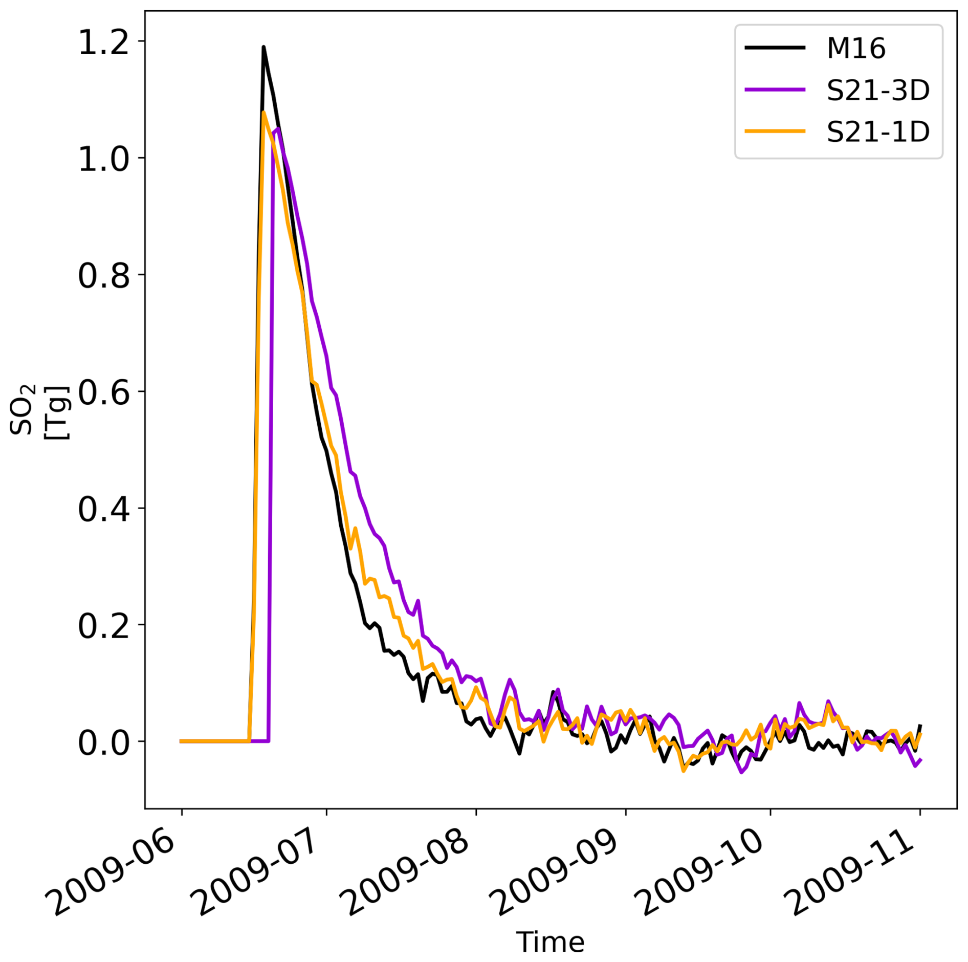
Figure 2 Global evolution of volcanic SO₂ in the M16, S21-1D, and S21-3D simulations. To isolate the volcanic SO₂, we have subtracted the SO₂ levels in the No-Volc simulation from the other three simulations. The date format is year-month.

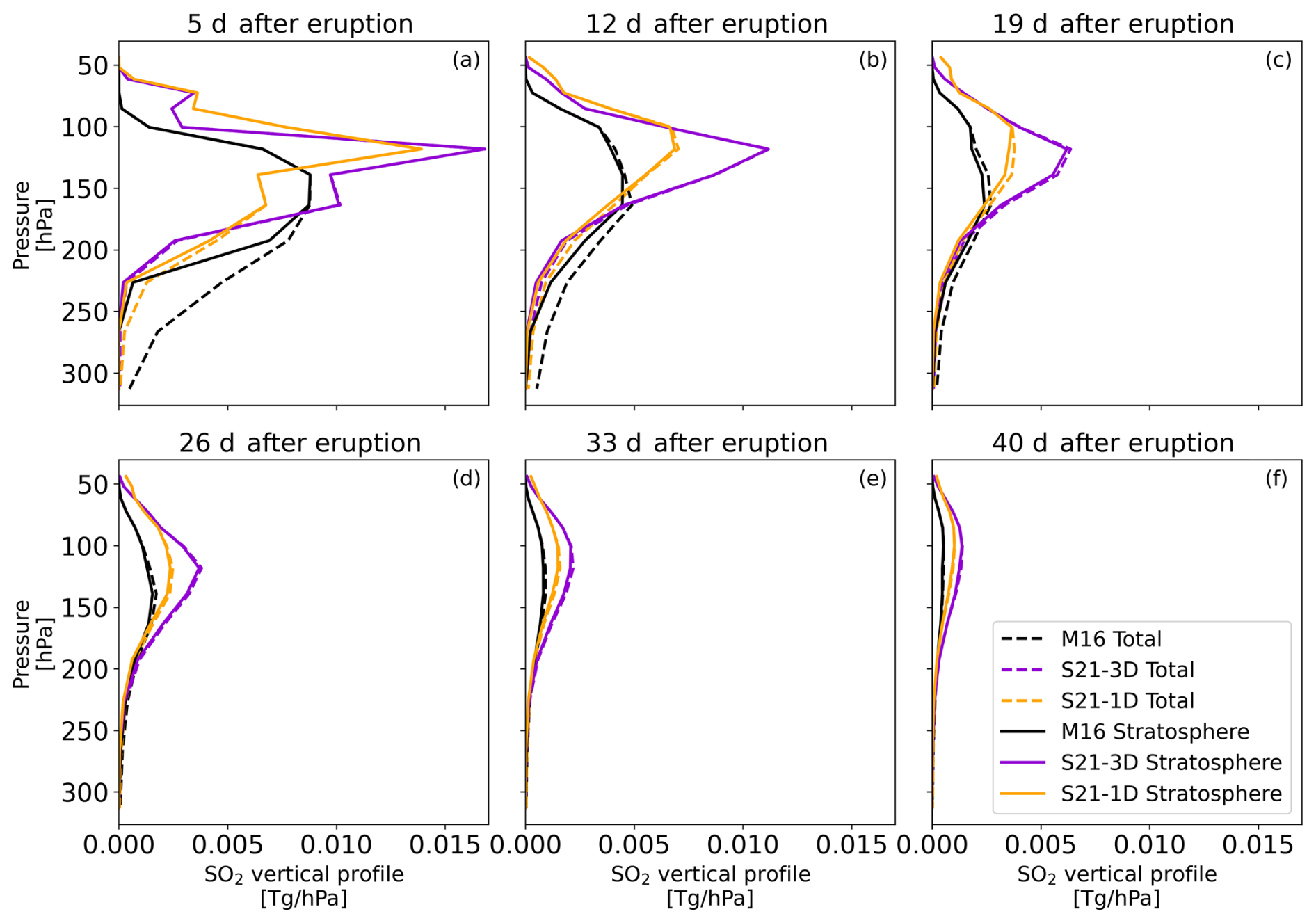
Figure 3 Vertical profiles for the global total volcanic SO₂ at (a) 5, (b) 12 , (c) 19, (d) 26, (e) 33, and (f) 40 d after the volcanic eruption on 15 June. The dashed lines represent the total amount of volcanic SO₂ in the atmosphere, whereas the solid lines represent the total amount of volcanic SO₂ in the stratosphere. To isolate the volcanic SO₂, we have subtracted the SO₂ levels in the No-Volc simulation from the other three simulations.

2.4 Aerosol data – satellite-derived aerosol extinction coefficients

The model simulations were compared with aerosol extinction data compiled from satellite observations retrieved by the spaceborne lidar CALIOP. The sensor acquired data at 532 and 1064 nm and had a polarization filter to retrieve depolarization data at 532 nm. We used nighttime data in the latest version of the lowest level available, i.e., Level 1B v4-51 (Product CAL_LID_L1-Standard-V4-51). Data were screened for ice clouds in the lowest 3 km of the stratosphere using depolarization ratios, and polar stratospheric cloud data were removed using a temperature threshold of 195 K outside 60° S–60° N (for details, see Friberg et al., 2018, 2023; Martinsson et al., 2022). Backscattering coefficients were computed by correcting for light attenuation by particles and molecules (including ozone) throughout the stratosphere (Friberg et al., 2018, 2023; Martinsson et al., 2022). Extinction coefficients were computed using a lidar ratio of 50 sr, i.e., a typical extinction-to-backscattering value for volcanic aerosol (Jäger and Deshler, 2002, 2003).

3 Results and discussion

3.1 Temporal and spatial evolution of volcanic SO₂

The differences in the vertical SO₂ distribution between M16 and the S21 datasets are retained after interpolation onto the rather coarse model grid (see Fig. S1 in the Supplement). The S21 datasets show that half of the SO₂ was injected to pressure levels below <150 hPa and almost all SO₂ was injected to the stratosphere, whereas M16 injected a large portion of the SO₂ into the upper troposphere (UT). The injected volcanic SO₂ profiles in the three simulations result in a large difference in SO₂ lifetime. Figure 2 shows the increase in global SO₂ load in the atmosphere following the June 2009 eruptions of Sarychev Peak. The volcanic SO₂ from M16 and S21-1D was injected on 15 and 16 June with a total of 1.2 Tg for the M16 and 1.09 Tg for the S21-1D dataset. For S21-3D, SO₂ was injected on 19 June with a total mass of 1.09 Tg. The global volcanic SO₂ levels for the M16 simulation (Fig. 2, black line) drop to levels below the simulations with S21-1D and S21-3D (orange and purple lines) by the beginning of July, regardless of the 0.11 Tg higher injected SO₂ mass in M16. The more rapid removal occurs since a large fraction of SO₂ in M16 is injected at altitudes below the tropopause, where the SO₂ is subject to the rapid wet chemistry of the troposphere, causing the SO₂ to be removed more quickly compared to the S21-1D and S21-3D datasets (Fig. 3).

In the S21-1D and S21-3D simulations, more than 95 % of the total SO₂ mass was injected into the stratosphere, whereas only 75 % of the SO₂ was injected into the stratosphere in the M16 simulation.

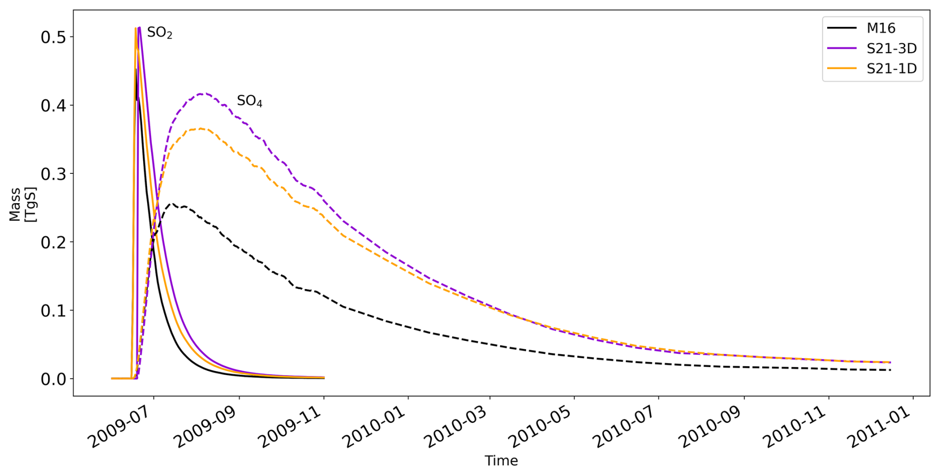
Figure 4 Stratospheric evolution of the amount of sulfur for SO₂ (solid lines) and SO₄ in the particle phase (dashed lines) over time, with daily values for both SO₂ and SO₄ till the end of October 2009 and monthly values for SO₄ from November 2009 to December 2010. To isolate the volcanic SO₂ and SO₄, we have subtracted the SO₂ and SO₄ levels in the No-Volc simulation from the other three simulations. The date format is year-month.

The time evolution of the vertical distribution of the SO₂ concentration is shown in Fig. 3. The volcanic SO₂ is seen at six different times: (a) 5, (b) 12, (c) 19, (d) 26, (e) 33, and (f) 40 d after the volcanic eruption on 15 June. Both the stratospheric SO₂ mass (solid lines) and the total atmospheric (tropospheric + stratospheric) SO₂ mass (dashed lines) are shown. Figure 3a shows SO₂ profiles for the first date when all the SO₂ has been emitted in all simulations. It can be seen that even though the model resolution is coarser than that of the S21 input datasets, there is still a structure with high SO₂ concentrations in narrower layers than in M16. Moreover, a large fraction of the SO₂ mass at lower altitudes is located in the troposphere in the M16 simulation. This is seen in Fig. 3a, where the dashed line deviates from the stratospheric mass (solid line). The tropospheric SO₂ is removed rapidly, shown by the difference between the dashed and solid line for the M16 simulation, where most tropospheric SO₂ had already been removed 12 d after the eruption (Fig. 3b). There is very little difference between the solid and dashed lines for the S21 simulations, demonstrating that most of this SO₂ is injected into the stratosphere. Not only is a larger fraction of SO₂ in the S21 simulations located in the stratosphere, but also the stratospheric SO₂ is located at a higher altitudes, i.e., deeper into the stratosphere. This leads to higher SO₂ concentrations in the S21 simulations, in particular between 100 and 200 hPa. Additionally, the horizontal SO₂ distribution impacts the lifetime of the SO₂. In M16, SO₂ is spread more towards the subtropics (Fig. S2), where the tropopause is located at high altitudes, likely leading to more rapid cross-tropopause transport, reducing the stratospheric SO₂ mass.

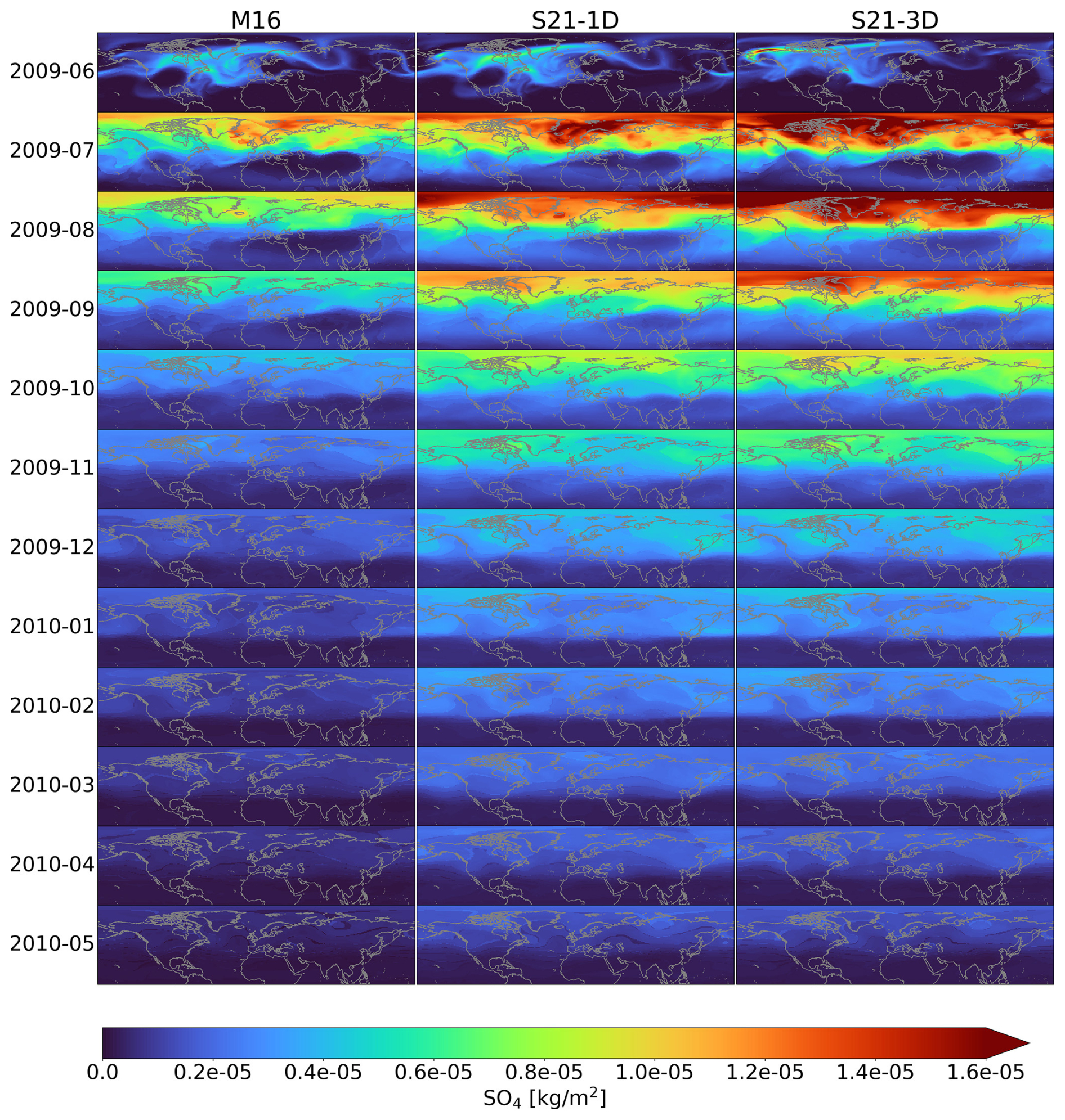
Figure 5 Monthly mean of stratospheric SO₄ in the NH during the first year after the volcanic eruption. To isolate the volcanic SO₄, we have subtracted the SO₄ levels in the No-Volc simulation from the other three simulations. The date format is year-month.

Even though the vertical SO₂ profiles for the two S21 datasets are rather similar after 5 d, there is a pronounced difference in the maximum SO₂ concentrations up to 1 month after the simulation (Fig. 3). The difference between the two S21 simulations is most likely a result of differences in the horizontal spread of the SO₂ in the two simulations, where SO₂ in S21-1D is transported more towards the subtropics, leading to more cross-tropopause transport for S21-1D than S21-3D. This exemplifies the sensitivity of the transport of the volcanic aerosol to air movement and weather patterns. Simulations of volcanic climate impact are often run with single-column data of SO₂, where the volcanic injections are represented by vertical columns in single geographical (latitude × longitude) grid cells. Small errors/uncertainties in simulated air dynamics can result in vast differences in the geographical spread of the volcanic SO₂, leading to under- or overestimation of the aerosol lifetime and resulting climate cooling (e.g., Tilmes et al., 2023). Using the S21-3D dataset from satellite observations a few days after the eruption, when the initial transport has already taken place, reduces the importance of the models' ability to correctly simulate the air movement at the time of the eruption.

3.2 Temporal and spatial evolution of volcanic SO₄

The injected SO₂ is converted to SO₄ over the first weeks after the injection. Figure 4 shows the resulting increase in SO₄ after the volcanic eruption together with the decreasing SO₂ in the stratosphere. The peak mass for SO₄ differs in both time and magnitude for the three simulations. In the M16 simulation, SO₄ peaks in mid-July, 4 weeks after the eruption. The S21-1D and S21-3D volcanic SO₄ peaks in August, approximately 8 weeks after the eruption.

The earlier peak date for M16 than S21-1D and S21-3D stems from the difference in their vertical profiles of SO₂, where S21-1D and S21-3D injected more SO₂ to higher altitudes. In M16, a larger fraction of the SO₂ is injected into the first few kilometers above the tropopause. Both the injected SO₂ and the resulting aerosol formed at these lower altitudes are transported out of the stratosphere more quickly than SO₂ and aerosol located at the higher altitudes, explaining the longer-lasting SO₄ and later peak for S21-1D and S21-3D. The SO₄ mass for S21-3D is already substantially larger than for M16 by July and remains higher throughout fall. In November, the SO₄ mass is almost twice as high for S21-3D compared with M16, indicating a substantially larger volcanic climate impact in the S21-3D simulation. The SO₄ mass 1.5 years after the eruption, in December 2010, is still elevated for all three simulations. The S21 datasets have, however, an almost double amount of SO₄ mass at the end of 2010 compared with the M16 simulations.

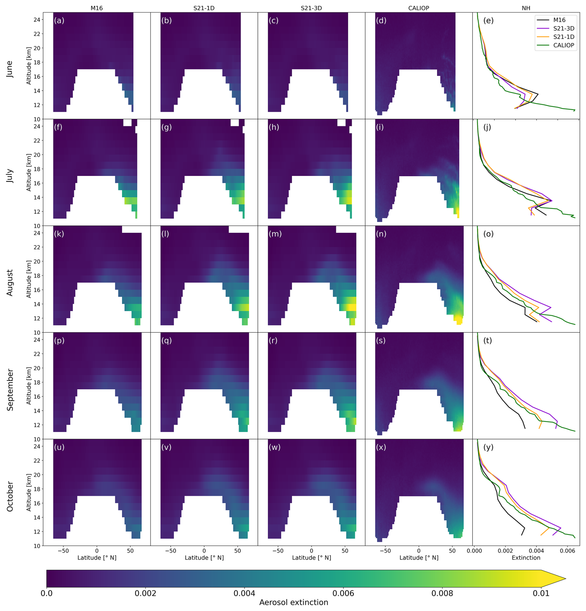
Figure 6 Zonal monthly mean stratospheric evolution of the aerosol extinction coefficient for the three simulations and satellite observations from CALIOP. The first three columns show the simulations (M16, S21-1D, and S21-3D), and the fourth column represents the CALIOP observations. The fifth column shows the average vertical aerosol extinction profiles in the NH for both simulations and the observations. The rows correspond to different months, from June to November 2009. The white areas are excluded values located in the troposphere and missing latitudes in CALIOP. Note that the simulations have a wavelength of 550 nm, whereas CALIOP observations have a wavelength of 532 nm.

The large differences in volcanic sulfate aerosol loading over time are also visible in Fig. 5. The initial transport of the volcanic SO₂ results in different patterns in the SO₄ load between the datasets emitted as a single column and the S21-3D dataset. After this, the pattern of the SO₄ load is similar between the simulations but aerosol concentrations drop off more rapidly in the M16 simulation compared to the S21 datasets. The aerosol is mainly located at middle and high latitudes for all three simulations, but there is substantial equatorward transport during the NH fall and winter after the eruption.

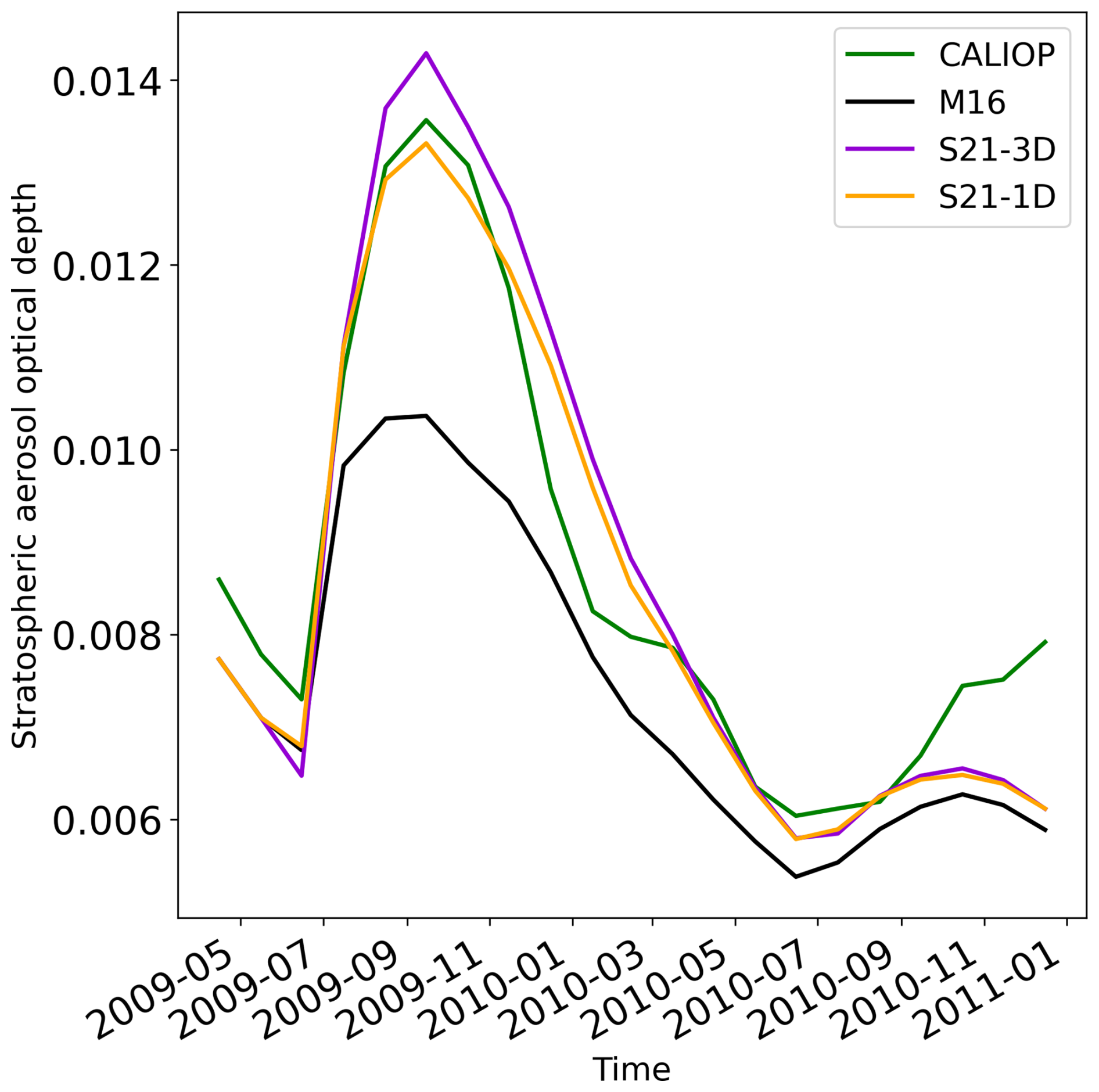
Figure 7 Global mean stratospheric aerosol optical depth (AOD) for the three simulations – M16, S21-3D, and S21-1D – compared with observations by CALIOP. Note that the simulations show AOD at 550 nm, whereas CALIOP observations provide AODs at a wavelength of 532 nm. The date format is year-month.

Figure 8 Global geometric mean stratospheric aerosol effective radius (a) and stratospheric AOD divided by stratospheric SO₄ mass (b) for the four simulations: M16, S21-3D, S21-1D, and No-Volc. The date format is year-month.

3.3 Comparison with CALIOP observations

Here we will compare the simulations with aerosol observations from the spaceborne lidar CALIOP. This comparison is done for the aerosol extinction coefficient (Fig. 6) and AOD (Fig. 7). The first four columns in Fig. 6 represent simulations with the three datasets – M16, S21-1D, and S21-3D – and CALIOP observations, where each row corresponds to monthly zonal mean values from June to November 2009. The fifth column in the figure shows the average aerosol extinction over all longitudes in the NH, i.e., extinction profiles. Since CALIOP is a polar-orbiting satellite and only nighttime data from CALIOP are used in this study, there are missing data at high latitudes in the NH, in particular during the summer months. We have removed the data from the missing latitudes for all simulations to enable a direct comparison. We have also introduced a common tropopause mask to ensure that we compare data from the same latitudes and altitudes. All model simulations initially show lower extinction values in the lowermost troposphere than the CALIOP observations. Averaging data in the proximity of the tropopause is complicated due to the strong concentration gradients in this altitude region. The satellite data contain a substantially higher vertical resolution of both the extinction data and the tropopause altitude than the models do. The coarser resolution of the model results in less sharp concentration gradients in the tropopause region. Moreover, for the simulations, the division between the stratospheric and tropospheric data was performed based on the maximum probability of the daily chemical tropopause, which results in some of the lowest-stratosphere data including influence from tropospheric air, thus lowering the extinction values. Above these lowest altitudes, the model simulations have extinction coefficients similar to those of the CALIOP observations. During July, the M16 profiles bear most resemblance to the CALIOP profiles, but after this month, the profiles from the S21 simulations have values more similar to the CALIOP observations.

There are clear differences in the altitude–latitude distributions among the three simulations, where the S21 simulations show higher extinction coefficients in the northern midlatitude lowermost stratosphere (LMS). Aerosol, in all simulations, spreads to the tropics but not to as high altitudes in the M16 simulations as in the S21 simulations. This is expected due to the generally lower injection altitudes for the simulations with the M16 SO₂ dataset. The simulations predict lower extinction coefficients in the lowest kilometers of the northern midlatitudes and larger volcanic influence at higher altitudes. CALIOP shows the highest extinction coefficients at low altitudes, which is expected due to the higher pressure there. Furthermore, CALIOP shows that almost all aerosol remained below 20 km altitude. Thus, it did not reach the upper branch of the Brewer–Dobson (BD) circulation. Even though there are some differences between the three simulations and the CALIOP observations, the general patterns are similar. The Sarychev eruption (i) influenced mainly the midlatitudes, (ii) was almost isolated within the NH, and (iii) did not enter the deep BD branch.

The extinction coefficients for the simulations and observations start to attain similar values and gradients at most altitudes in August, following the initial phase of SO₂ transformation and particle formation (June–July), with M16 showing the lowest extinction coefficients. The S21 simulations continue to agree with observations in the following 2 months, whereas M16 starts to deviate more from the observations and shows lower extinction coefficients than both observations and the S21 simulations. This pattern is most pronounced in the LMS, illustrating the influence of outflow from the stratosphere, which leads to the lower AODs for M16 than for the S21 observations.

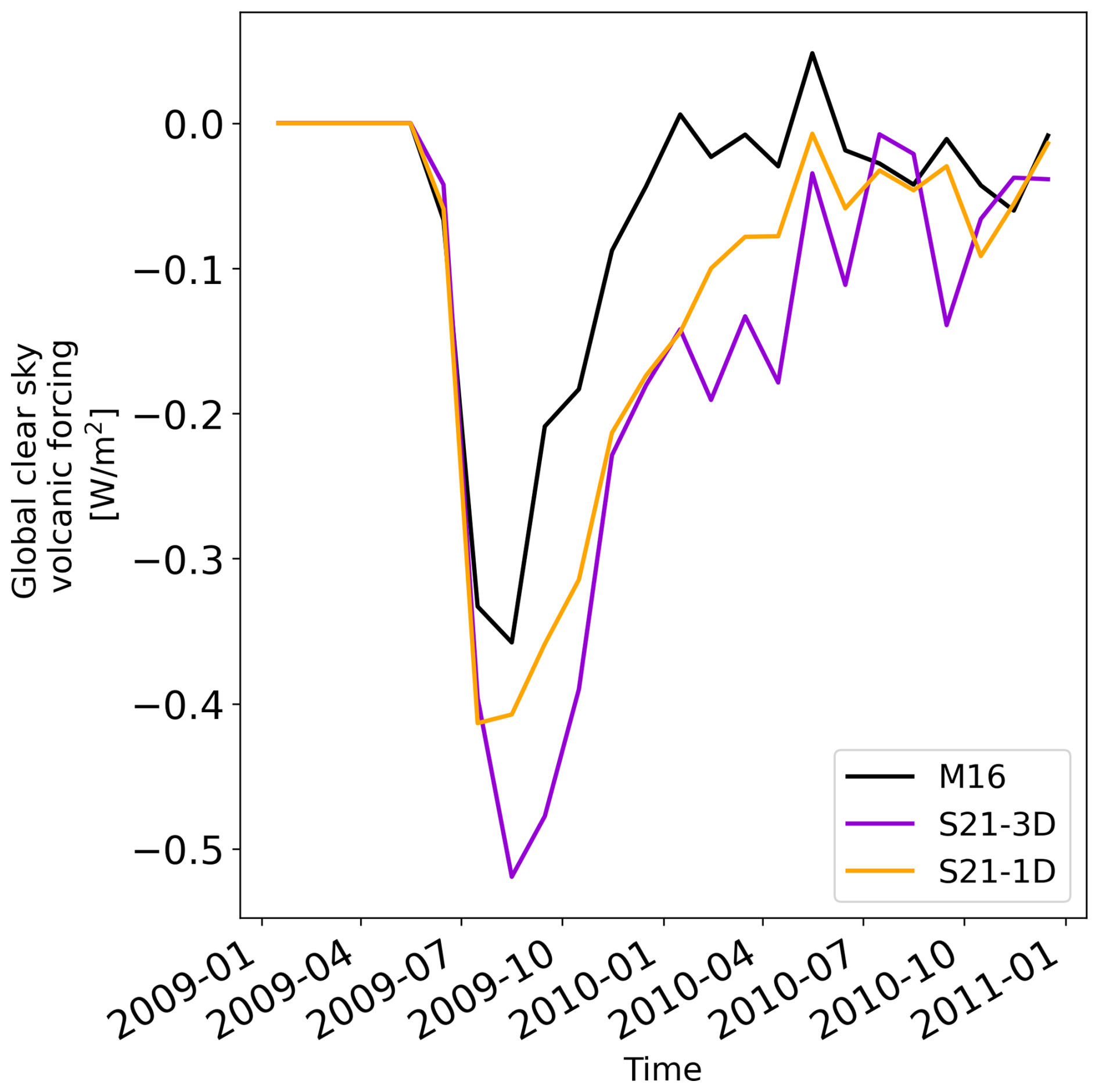
Figure 9 Global clear-sky volcanic forcing from the Sarychev eruption for the three model simulations. The date format is year-month.

Table 2 Global average volcanic effective radiative forcing (ERF) for the three simulations for different time periods.

The resulting stratospheric AOD from the extinction profiles is shown in Fig. 7. The S21-1D simulation shows the best agreement with CALIOP at almost all times. The S21-3D simulation peaks at higher values than CALIOP, while M16 displays an increase in stratospheric AOD after the Sarychev eruption which is approximately 60 % of that seen in CALIOP. The climate effects of stratospheric aerosol are dependent not only on the SO₄ mass but also on where in the size distribution the SO₄ is placed, since particles of different sizes reflect different amounts of solar radiation (Laakso et al., 2022; Tilmes et al., 2023). We investigated this by calculating the average stratospheric aerosol effective radius (r_e) over time for all simulations (Fig. 8a). The initial response during the first few weeks after the eruption is a decrease in r_e, which is followed by an increase in r_e over the next months. The decrease and increase are largest in S21-3D and smallest in M16. The No-Volc simulation displays a decrease over time since there is particle shrinkage after the Kasatochi eruption that occurred in August 2008.

To investigate the impact of the size distribution changes on the AOD, we have divided the stratospheric AOD by the total stratospheric SO₄ mass (see Fig. 8b). This quantity illustrates whether the amount of light reflected per SO₄ mass varies between the simulations. When the eruption occurs, the $\mathrm{AOD}/{\mathrm{SO}}_{\mathrm{4}}$ ratio decreases for all three volcanic simulations, with the largest decrease in the S21-3D simulation. Hence, the higher AOD values in the S21-3D simulation cannot be explained by a greater efficiency in light reflection for the SO₄ mass, pointing to cross-tropopause transport as the major cause of difference in AOD among the simulations.

3.4 Radiative forcing – comparison of simulations

Finally, we will evaluate the extent of volcanic climate cooling estimated by the three simulations. Figure 9 shows the global clear-sky volcanic effective radiative forcing for the simulations. The effective radiative forcing (ERF) was calculated using the method suggested by Ghan (2013), which has previously been used for calculations of volcanic forcing by Schmidt et al. (2018). The S21-3D simulation, run with SO₂ at high vertical and horizontal resolution, predicts the highest and longest impact on the global volcanic forcing. The dataset with only high vertical resolution but released in a single column, S21-1D, follows the curve of S21-3D closely but with slightly lower values. The dataset with low vertical resolution, M16, has the weakest global clear-sky volcanic forcing, which disappears more rapidly compared to the other two simulations. The peak value for the M16 simulation is −0.36 W m⁻² in August, the peak value for S21-1D is −0.41 W m⁻² in July, and the peak value for S21-3D is −0.52 W m⁻² in August. The long-term forcing differed more among the models. The forcing during the first year post-eruption was more than twice as high for S21-3D than for simulations with the models' default dataset, M16, i.e., −0.24 and −0.11 W m⁻², respectively (Table 2). This large difference exemplifies the importance of the vertical placement of volcanic SO₂ injections in global climate models.

4 Conclusions

We have simulated the Sarychev eruptions' impact on the stratosphere and climate, using three different SO₂ injection profiles in WACCM (Whole Atmosphere Community Climate Model). The eruptions positioned SO₂ throughout the lower stratosphere and upper troposphere, in an altitude range of 11–19 km, increasing the stratospheric aerosol load (AOD) by 100 % in the months following the SO₂ injection. The overarching goal of this work was to investigate the influence of vertical SO₂ distributions on the stratospheric aerosol load and climate. To this end, we compared our simulations with high-vertical-resolution observations from the satellite-borne lidar instrument CALIOP.

WACCM simulations with the S21 SO₂ datasets captured the AOD well in the aftermath of the June 2009 Sarychev eruptions. Simulations with these datasets produced temporal evolution in stratospheric AODs very similar to that of observations from the satellite-borne high-vertical-resolution lidar instrument CALIOP. Furthermore, the simulated vertical distribution of the aerosol load, expressed by the aerosol extinction coefficients, agreed well with the CALIOP observations. On the other hand, simulations with the default volcanic injection dataset showed generally lower aerosol extinction coefficients and AODs.

Simulations with the S21-3D SO₂ dataset produced more than twice as strong volcanic forcing as the default dataset in WACCM. The global clear-sky radiative forcing during the first year after eruption amounted to −0.24 (−0.11) W m⁻² for the high-resolution (low-resolution) dataset. Although it holds 10 % more SO₂, the default dataset induces far less climate cooling than the high-resolution datasets do. These findings highlight the need to produce datasets of volcanic SO₂ injections to the stratosphere that precisely place the SO₂ at correct altitudes, especially when the eruptions reach the lowermost stratosphere. Moreover, the results indicate that our present understanding of volcanic climate cooling is in part limited by the SO₂ profiles, and it is highly likely that it is not only the Sarychev eruptions' climate cooling that is underestimated due to inaccurate assumptions about SO₂ profiles. Climate cooling of pre- and post-Sarychev eruptions may, to varying degrees, be under- or overestimated due to limited knowledge of the SO₂ vertical profiles. This highlights the need for further investigations of volcanic SO₂ profiles. Our study required high-vertical-resolution satellite retrievals of aerosols which have, until the present, only been accomplished by lidar. CALIOP provided us with such data from 2006–2023. This study highlights the usefulness of spaceborne lidar systems and the need for continuous atmospheric observations from such systems, and it exemplifies the need for future spaceborne lidars.