Evaluating present-day and future impacts of agricultural ammonia emissions on atmospheric chemistry and climate

Agricultural practices are a major source of ammonia (NH₃) in the atmosphere, which has implications for air quality, climate, and ecosystems. Due to the rising demand for food and feed production, ammonia emissions are expected to increase significantly by 2100 and would therefore impact atmospheric composition such as nitrate (${\mathrm{NO}}_{\mathrm{3}}^{-}$) or sulfate (${\mathrm{SO}}_{\mathrm{4}}^{\mathrm{2}-}$) particles and affect biodiversity from enhanced deposition. Chemistry–climate models which integrate the key atmospheric physicochemical processes with the ammonia cycle represent a useful tool to investigate present-day and also future reduced nitrogen pathways and their impact on the global scale. Ammonia sources are, however, challenging to quantify because of their dependencies on environmental variables and agricultural practices and represent a crucial input for chemistry–climate models. In this study, we use the chemistry–climate model LMDZ–INCA (Laboratoire de Météorologie Dynamique–INteraction with Chemistry and Aerosols) with agricultural and natural soil ammonia emissions from a global land surface model ORCHIDEE (ORganising Carbon and Hydrology In Dynamic Ecosystems), together with the integrated module CAMEO (Calculation of AMmonia Emissions in ORCHIDEE), for the present-day and 2090–2100 period under two divergent Shared Socioeconomic Pathways (SSP5-8.5 and SSP4-3.4). Future agricultural emissions under the most increased level (SSP4-3.4) have been further exploited to evaluate the impact of enhanced ammonia emissions combined with future contrasting aerosol precursor emissions (SSP1-2.6 – low emissions; SSP3-7.0 – regionally contrasted emissions). We demonstrate that the CAMEO emission set enhances the spatial and temporal variability in the atmospheric ammonia in regions such as Africa, Latin America, and the US in comparison to the static reference inventory (Community Emissions Data System; CEDS) when assessed against satellite and surface network observations. The CAMEO simulation indicates higher ammonia emissions in Africa relative to other studies, which is corroborated by increased current levels of reduced nitrogen deposition (NH_x), a finding that aligns with observations in west Africa. Future CAMEO emissions lead to an overall increase in the global NH₃ burden ranging from 59 % to 235 %, while the ${\mathrm{NO}}_{\mathrm{3}}^{-}$ burden increases by 57 %–114 %, depending on the scenario, even when global NO_x emissions decrease. When considering the most divergent scenarios (SSP5-8.5 and SSP4-3.4) for agricultural ammonia emissions, the direct radiative forcing resulting from secondary inorganic aerosol changes ranges from −114 to −160 mW m⁻². By combining a high level of NH₃ emissions with decreased or contrasted future sulfate and nitrate emissions, the nitrate radiative effect can either overcompensate (net total sulfate and nitrate effect of −200 mW m⁻²) or be offset by the sulfate effect (net total sulfate and nitrate effect of $+\mathrm{180}\mathrm{mW}{\mathrm{m}}^{-\mathrm{2}}$). We also show that future oxidation of NH₃ could lead to an increase in N₂O atmospheric sources from 0.43 to 2.10 Tg N₂O yr⁻¹ compared to the present-day levels, representing 18 % of the future N₂O anthropogenic emissions. Our results suggest that accounting for nitrate aerosol precursor emission levels but also for the ammonia oxidation pathway in future studies is particularly important to understand how ammonia will affect climate, air quality, and nitrogen deposition.

1 Introduction

Ammonia (NH₃) is a key atmospheric species playing a crucial role in the alteration of air quality and climate through its implication in airborne particle matter formation (PM or aerosols) (Anderson et al., 2003; Bauer et al., 2007). The resulting aerosols, namely ammonium nitrates or ammonium sulfates, have important impacts on the Earth's radiative budget due to their ability to scatter the incoming radiation, act as cloud condensation nuclei, and indirectly increase cloud lifetime (Abbatt et al., 2006; Henze et al., 2012; Behera et al., 2013; Evangeliou et al., 2021). Through dry and wet deposition processes, NH₃ and ${\mathrm{NH}}_{\mathrm{4}}^{+}$ are also responsible for adverse damages to the ecosystems, including biodiversity loss (Stevens et al., 2020; Guthrie et al., 2018; de Vries, 2021).

Agriculture and, more specifically, livestock manure management and land fertilization account for 85 % of NH₃ sources (Behera et al., 2013). Because the volatilization of NH₃ is highly dependent on soil temperature and humidity, land surface models (LSMs) are promising to estimate NH₃ emissions at the global scale. Recently, in Beaudor et al. (2023a), a specific LSM module dedicated to agricultural ammonia emissions (CAMEO; Calculation of AMmonia Emissions in ORCHIDEE) has been presented and evaluated against satellite-derived emission fluxes. CAMEO is a process-based model in which emissions from livestock management, grazing, and N fertilization (as well as natural soil sources) are interactively calculated within the ORCHIDEE LSM (ORganising Carbon and Hydrology In Dynamic Ecosystems; Vuichard et al., 2019). CAMEO-based seasonal variation in NH₃ emissions, which depend on both meteorological and agricultural practices, highlights very satisfying correlation scores with satellite-based emissions, as demonstrated in Beaudor et al. (2023a, 2025). In addition, the ability of CAMEO to simulate natural soil emissions is useful since up to now they have been poorly quantified at the global scale and appear a non-negligible source in specific regions such as Africa. Livestock activities and synthetic fertilizer use are projected to intensify in the following decades, leading to a potential crucial NH₃ emission increase (Bodirsky et al., 2012; Popp et al., 2017; Beaudor et al., 2025). Impacts of the NH₃ emissions on the future nitrate aerosol formations and climate have already been assessed in Hauglustaine et al. (2014) under Representative Concentration Pathway (RCP) scenarios until 2100 using the global climate–chemistry atmospheric model LMDZ–INCA (Laboratoire de Météorologie Dynamique–INteraction with Chemistry and Aerosols). They have illustrated the substantial impact of NH₃ emissions on the future formation of nitrate aerosols and on direct radiative forcing (Hauglustaine et al., 2014). By the year 2100, due to significant emissions from agriculture, the contribution of nitrate aerosol to the anthropogenic aerosol optical depth could increase by as much as 5-fold under the most impactful scenario considered. RCP scenarios have also been exploited to study the importance of future atmospheric NH₃ on chemistry and climate, with a special focus on atmospheric NH₃ losses including oxidation processes (Paulot et al., 2016; Pai et al., 2021). The ammonia oxidation pathway mentioned is a direct contributor to nitrous oxide (N₂O) emissions in the atmosphere, which is a potent greenhouse gas. Future losses of nitrous oxide could increase significantly due to intensified agricultural emissions and the emerging hydrogen fuel economy, which heavily relies on ammonia as an energy carrier Hauglustaine et al. (2014); Bertagni et al. (2023). Recently, in Phase 6 of the Coupled Model Intercomparison Project (CMIP6) framework, socioeconomical drivers have gained greater importance and have been incorporated into a new set of scenarios called SSPs (Shared Socioeconomic Pathways) (O'Neill et al., 2016). The Sixth Assessment Report from the Intergovernmental Panel on Climate Change (IPCC) covers a broader range of greenhouse gas and air pollutant trajectories through the use of SSP scenarios (Intergovernmental Panel On Climate Change, 2023). However, future agricultural NH₃ emissions that have been prescribed for the Sixth Assessment Report have several limitations regarding the consideration of climate and livestock densities as described in Beaudor et al. (2025). Livestock distribution, which is considered an important driver of future NH₃ emissions, has been recently projected up to 2100 following a unique downscaling method (Beaudor et al., 2025). In this latter study, CAMEO has been exploited to calculate future NH₃ emissions accounting for the evolution of climate, livestock, and N fertilizers.

By demonstrating encouraging results for the present day, especially when compared to reference inventories, CAMEO emissions open promising perspectives to represent ammonia and related aerosols within chemistry–climate models. Like most chemistry–climate models, LMDZ–INCA relies on the seasonally forced inventory called CEDS (Community Emissions Data System; McDuffie et al., 2020). We hypothesize that prescribing CAMEO emissions instead of CEDS for agricultural sources could improve the simulated atmospheric species and aerosol concentrations, as well as N deposition fluxes, especially over Africa, with important differences in the NH₃ emissions that have been demonstrated previously (Beaudor et al., 2023a). In the present paper, we introduce the impact of the new present-day and future CAMEO emission datasets on atmospheric chemistry using the global LMDZ–INCA model. As a first global and regional evaluation, the columns simulated by LMDZ–INCA with CAMEO and CEDS inventories for the present day have been compared to the NH₃ columns observed by the Infrared Atmospheric Sounding Interferometer (IASI) satellite instrument. Statistics involving ground-based measurements of surface concentrations (trace gases: NH₃ and NO₂; ionic species: ${\mathrm{NH}}_{\mathrm{4}}^{+}$, ${\mathrm{NO}}_{\mathrm{3}}^{-}$, and ${\mathrm{SO}}_{\mathrm{4}}^{\mathrm{2}-}$) have also been performed to ensure a more robust evaluation of the model.

For the first time, we propose the investigation of how future agricultural NH₃ emissions, influenced by climate change, livestock management, and nitrogen fertilizer use, will impact atmospheric chemistry and climate (kept at present-day conditions). We assess the effects of future emissions under SSP4-3.4 and SSP5-8.5, which represent the scenarios with the most and least significant global increases by the year 2100. SSP4-3.4 and SSP5-8.5, describing, respectively, “A world of deepening inequality”, and “Fossil-fueled Development – Taking the Highway” (Calvin et al., 2017; Kriegler et al., 2017), reflect divergent agricultural drivers. In the first place, SSP4-3.4 represents the scenario with the weakest evolution of livestock, while SSP5-8.5 shows the most significant increase among all Shared Socioeconomic Pathways (SSPs), according to Riahi et al. (2017). In line with these trends, the fossil-fuel-intensive scenario SSP5-8.5 also experiences the highest demand and production of food and feed crops among the three scenarios considered, as noted by Beaudor et al. (2025). This increase occurs despite low population growth and is driven by the prevalence of diets high in animal products (Fricko et al., 2017; Kriegler et al., 2017). Despite the peak in food and feed crop production, projected fertilizer applications in SSP5-8.5 rise only slightly. This is attributed to the minimal production of biofuel crops, a result of the lack of climate mitigation policies and rapid advancements in agricultural productivity. In contrast, SSP4-3.4 exhibits the highest use of fertilizer and reveals significant regional differences, with high-consumption lifestyles among elite socioeconomic categories and low-consumption levels for the rest of the population (Calvin et al., 2017).

Through knowing the importance of sulfate dioxide (SO₂) and nitrogen oxide (NO_x) emissions for nitrate and sulfate aerosol formation (Hauglustaine et al., 2014; Lachatre et al., 2019), scenarios have been designed to evaluate the impact of future NH₃ emissions under contrasted SO₂ and NO_x conditions. In this paper, we present six simulations from LMDZ–INCA, including two present-day simulations, with CEDS and CAMEO inventories for NH₃ emissions and four future simulations over 2090–2100 with future NH₃ emissions from CAMEO and other sources at different future levels (i.e., globally decreased and regionally contrasted level of emissions). The paper is organized as follows: in Sect. 2, we present the emission inventories prepared and considered in the global chemistry–climate model for the present-day and future (2100) simulations. In Sect. 3, we describe the LMDZ–INCA chemistry–climate model used, along with modeling setup. Section 4 presents the simulated NH₃ columns and the N deposition fluxes for the present day, including an evaluation of the model performance with IASI and ground-based measurements. In Sect.5, the perturbations associated with future agricultural emissions on atmospheric chemistry and climate under different scenarios are illustrated. Finally, in Sect. 6, we draw the conclusions from this work.

2 Emission datasets

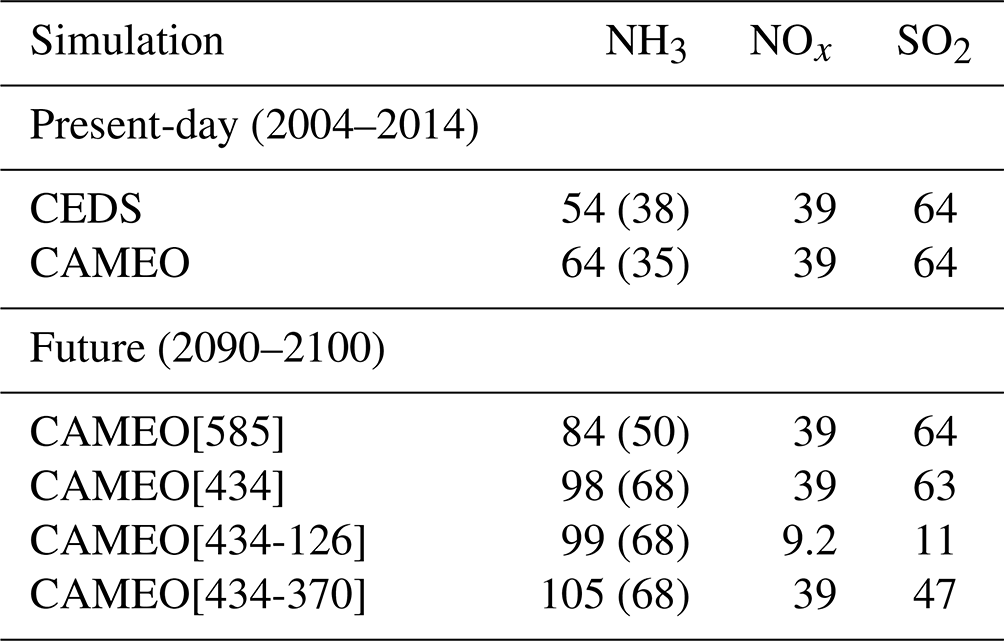
In this work, we focus on the impact of agricultural NH₃ emissions calculated from CAMEO on atmospheric chemistry. Therefore, specific attention is given to the modeling of these emissions, which are further detailed in the two following sub-sections. Please note that except for the agricultural and land-related NH₃ emissions, all the other anthropogenic sources used in this study are based on the same sets of data (i.e., derived from the CMIP6 exercise both for present-day (CEDS) and future scenarios; McDuffie et al., 2020; Gidden et al., 2018). Emissions from biomass burning, including small fires from agricultural waste burning, come from the Global Fire Emissions Database (GFED4s) inventory (van der Werf et al., 2017). NH₃ emissions from fire account for 4.2 Tg N yr⁻¹ for the historical period (this source is excluded from the values in Table 1). The global anthropogenic NH₃, NO_x, and SO₂ emissions used in the study are presented in Table 1. For comparison, the EDGARv8.1 inventory (https://edgar.jrc.ec.europa.eu/index.php/dataset_ap81, last access: 12 February 2025) quantifies for all anthropogenic sectors a total of NH₃ emissions of 42 Tg N yr⁻¹ in 2010 (including 36 Tg N yr⁻¹ for the agricultural sector).

Table 1 Global anthropogenic ammonia (NH₃), nitrogen (NO_x), and sulfate (SO₂) emissions used for the present-day (2004–2014) and future (2090–2100) simulations. Agricultural NH₃ emissions are presented in parentheses. Please note that CAMEO emissions also include natural soil emissions (Tg N yr⁻¹ or Tg S yr⁻¹).

2.1 Present-day agricultural NH₃ emissions

Two present-day agricultural NH₃ emission datasets are tested. One simulation accounts for emissions from CEDS (McDuffie et al., 2020), and another one uses the estimated emissions from the CAMEO module included in the LSM ORCHIDEE described in Beaudor et al. (2023a). CAMEO simulates manure production and agricultural NH₃ emissions from the manure management chain (including manure storage and grazing) and soil emissions after fertilizer or manure application. CAMEO simulates interactive NH₃ emissions into the global LSM ORCHIDEE (Krinner et al., 2005; Vuichard et al., 2019). In addition, natural soil NH₃ emissions are also accounted for in CAMEO. ORCHIDEE represents the C and N cycles and simulates the water and energy fluxes within the ecosystems. The vegetation is represented by 15 plant functional types (PFTs), among which there are 2 crop types (C3 and C4) and 4 grass types (temperate, boreal, and tropical C3 grasses and a single C4 grass). ORCHIDEE is constrained by land-use maps, meteorological fields, and N input such as synthetic fertilizers. Livestock densities represent one of the most critical inputs for CAMEO since it is the main driver of the feed need estimation and, thus, of manure management and, to a lesser extent, soil emissions.

Emissions from agriculture are slightly lower in CAMEO compared to CEDS (35 vs. 38 Tg N yr⁻¹), but additional natural soil emissions account for 13 Tg N yr⁻¹. As a result, global annual NH₃ emissions from CAMEO are 10 Tg N yr⁻¹ higher than in CEDS (Table 1). Please note that due to a different set of input data, the agricultural ammonia emissions from the present study are 9 Tg N yr⁻¹ lower than the ones reported in the reference study (Beaudor et al., 2023a). This difference is mainly explained by the non-consideration of managed grasslands in the CMIP6 synthetic fertilizer forcing which led to a total fertilization input of 97 vs. 118 Tg N yr⁻¹ in the reference study. On another hand, the different climatic forcings may also impact the emissions. For self-consistency, CAMEO for the CMIP6 framework exploits the 3-hourly near-surface meteorological fields simulated by the Institut Pierre-Simon Laplace (IPSL) Earth system model (IPSL-CM6A-LR ESM) (Boucher et al., 2020) in the context of CMIP6 for near-surface air temperature, specific humidity, wind speed, pressure, short- and longwave incoming radiation, rainfall, and snowfall. The reference paper is based on the Climatic Research Unit (CRU) and Japanese Reanalysis (JRA) dataset (CRU–JRA V2.1) (Harris et al., 2014) (preprocessed and adapted by Vladislav Bastrikov, LSCE, personal communication, July 2020), provided at 6 h time steps.

2.2 Future emission scenarios

In this study, future emissions for different SSPs are used for the 2090–2100 period. CAMEO emissions for SSP5-8.5 and SSP4-3.4 have been exploited for future agricultural and natural NH₃ emissions in the CAMEO[SSPi] (SSPi includes 585, 434, 434-126, and 434-370) simulations, where agricultural sources account for 50 and 68 Tg N yr⁻¹ (respectively, for SSP5-8.5 and SSP4-3.4). SSP5-8.5 and SSP4-3.4 have been chosen primarily as they represent, respectively, the least and most important increase in NH₃ emissions estimated over 2090–2100 (Beaudor et al., 2025). The evolution of the global agricultural NH₃ emissions from the different SSPs from CAMEO under future climate is shown in Fig. S1 in the Supplement. These emission datasets have recently been constructed from a newly gridded livestock product and the use of the global process-based CAMEO before being evaluated against CMIP6 emissions developed by the Integrated Assessment Models (IAMs) in Beaudor et al. (2025). The future livestock distribution has, originally, been estimated until 2100 for three divergent SSPs (SSP2-4.5, SSP4-3.4, and SSP5-8.5) through a downscaling method based on regional livestock trends and future grassland areas (the detailed methodology can be found in Beaudor et al., 2025).

In addition to future CAMEO NH₃ emissions for SSP4-3.4 and SSP5-8.5, future CMIP6 emissions have been used for SSP1-2.6 and SSP3-7.0 (Gidden et al., 2018) for other emitted species but also for the anthropogenic sectors – other than agriculture – for NH₃ (waste, industry, etc.). These two SSPs were selected because they represent divergent scenarios for global NO_x and SO₂ emissions. SSP1-2.6 represents a “low” scenario, with air pollution and climate change being strongly mitigated. Emission regulations are implemented almost worldwide in various economic sectors such as energy generation, industrial processes, and transportation. In contrast, no climate change mitigation and only weak air pollution control are considered in SSP3-7.0. This scenario features contrasting emission trends, with strong regulations in the Northern Hemisphere and increasing emissions in the Southern Hemisphere. A slight difference in the NH₃ emissions is observable from CAMEO[434-126] and CAMEO[434-370] (Table 1). This difference is explained by the differences in the emissions from other anthropogenic sectors between SSP1.2-6 and SSP3-7.0. It is worth noting that even though future total NO_x emissions are similar between the present-day level and under SSP3-7.0 at the global scale, different regional patterns are observable (see Fig. S2).

Beaudor et al. (2025) demonstrate a global agreement between agricultural ammonia emissions developed by the IAMs and simulated with CAMEO. The global estimates from the IAMs inventories are, respectively, 50 and 66 Tg N yr⁻¹ under SSP5-8.5 and SSP4-3.4 compared to 50 and 68 Tg N yr⁻¹ for CAMEO. In this previous work, three interesting advantages are highlighted in favor of the use of CAMEO emissions:

• The consideration of environmental conditions (i.e., soil temperature and humidity, CO₂ increase, and vegetation changes).

• The consistent consideration of the key ammonia emission drivers (i.e., N input, meteorology, livestock, and land use) among all future SSPs, which is the result of the use of a single process-based model.

• The spatial heterogeneity is driven by environmental conditions and not kept constant over time within predefined regions using the information from the historical period.

• The incorporation of CAMEO into the land component of the IPSL ESM ensures better consistency throughout the various components, including LMDZ–INCA, paving the way for advancements in our understanding.

Considering the constraints of IAMs in precisely reflecting the primary factors influencing ammonia emissions, exploring their effects on atmospheric chemistry and climate beyond a global level appears unconvincing. We propose a hypothetical comparison based on the regional differences observed in the IPCC emissions and the CAMEO emissions projected for 2100. Figure S3 highlights the major regional differences between CMIP6 and CAMEO emissions in 2100 for the two considered SSPs (SSP4-3.4 and SSP5-8.5). The most distinguishable region is Africa, specifically North Africa's savanna combined with equatorial Africa, where the CMIP6 emissions for both SSPs are more than twice as high as those for CAMEO ($>\mathrm{15}\mathrm{Tg}\mathrm{N}{\mathrm{yr}}^{-\mathrm{1}}$). The primary explanation for this pattern lies in the simplified downscaling strategy adopted by the IAM method for projection. The approach applies a constant factor across the entire African continent over time, neglecting to account for regional influences such as livestock food expansion and changes in fertilizer application. Specifically, the northern Maghreb region is expected to play a significant role in the future, particularly under SSP4-3.4, as projections indicate an expansion in cultivated lands and fertilizer application, likely driven by the cultivation of bioenergy crops. As a consequence, one of the most expected differences between CMIP6 and CAMEO emission impacts would be a more enhanced production of aerosol formation and NO_y and NH_x deposition under CAMEO[434-370], where NO_x and SO₂ emissions are projected to increase compared to the present day in Africa. In contrast, in China, the smaller emission fluxes predicted by the IAMs under both SSPs compared to CAMEO indicate that we can expect a limitation or decrease in the formation of ammonium-related aerosols and therefore the resulting deposition, which would be stronger under CAMEO[434-126].

3 The LMDZ–INCA model

The LMDZ–INCA global chemistry–aerosol–climate model couples the LMDZ (Laboratoire de Météorologie Dynamique, version 6) general circulation model (GCM; Hourdin et al., 2020) and the INCA (INteraction with Chemistry and Aerosols, version 5) model (Hauglustaine et al., 2004, 2014). The interaction between the atmosphere and the continental surface is ensured through the coupling of LMDZ with the ORCHIDEE (version 1.9) dynamical vegetation model (Krinner et al., 2005). The present configuration is parameterized with the “standard physics” of the GCM (Boucher et al., 2020). The model incorporates 39 hybrid vertical levels extending up to 70 km, with a horizontal resolution of 1.3° in latitude and 2.5° in longitude. The GCM primitive equations are solved with a 3 min time step, large-scale transport of tracers is carried out every 15 min, and physical and chemical processes are calculated at 30 min time intervals.

The INCA model represents state-of-the-art CH₄-NO_x-CO-NMHC-O₃ tropospheric photochemistry (Hauglustaine et al., 2004; Folberth et al., 2006). The tropospheric photochemistry and aerosol scheme includes a total of 123 tracers, including 22 tracers representing aerosols. The model represents 234 homogeneous chemical reactions, 43 photolytic reactions, and 30 heterogeneous reactions. The tropospheric chemistry reactions are listed in Hauglustaine et al. (2004) and Folberth et al. (2006). Comparisons with observations have been extensively carried out to evaluate the gas phase version of the model in the lower stratosphere and upper troposphere. The distribution of aerosols is represented by considering anthropogenic sources such as sulfates, nitrates, black carbon (BC), and organic carbon (OC), as well as natural aerosols such as sea salt and dust. Reactions in the heterogeneous phase on both natural and anthropogenic tropospheric aerosols are also included (Bauer et al., 2004; Hauglustaine et al., 2004, 2014). A modal approach for the size distribution is used to track the number and mass of aerosols which is described by a superposition of five log-normal modes (Schulz, 2007). The particle modes are represented for three ranges: sub-micronic (diameter <1 µm), corresponding to the accumulation mode; micronic (diameter between 1 and 10 µm), corresponding to coarse particles; and super-micronic or super-coarse particles (diameter >10 µm). The diversity in the chemical composition, hygroscopicity, and mixing state is ensured by distinguishing soluble and insoluble modes. Specifically, soluble and insoluble aerosols are treated separately in both sub-micron and micron modes. Sea salt, SO₄, NO₃, and methane sulfonic acid (MSA) are treated as soluble components of the aerosol, and dust is treated as insoluble, whereas BC and OC appear in both the soluble and insoluble fractions. Ammonia and nitrate aerosols are represented through an extended chemical scheme that includes the ammonia cycle as described by Hauglustaine et al. (2014). The formation of the ammonium sulfate aerosols depends on the relative ammonia and sulfate concentrations and is characterized by three chemical domains (ammonium-rich, sulfate-rich, and very sulfate-rich conditions), as in Metzger et al. (2002). Extensive evaluations of the aerosol component of the LMDZ–INCA model have been carried out during the various phases of Aerosol Comparisons between Observations and Models (i.e., AeroCom; Gliß et al., 2021; Bian et al., 2017). Simulated surface NH₃, HNO₃, ${\mathrm{NH}}_{\mathrm{4}}^{+}$, ${\mathrm{SO}}_{\mathrm{4}}^{\mathrm{2}-}$, and ${\mathrm{NO}}_{\mathrm{3}}^{-}$ concentrations indicate satisfying performances when evaluated against observation network from the US, Europe, and Asia (Bian et al., 2017). The dry and wet deposition processes of ammonia, ammonium nitrate, and ammonium sulfate are described in Hauglustaine et al. (2004), with updated Henry's law coefficients taken from Sander (2023). Coarse nitrates on dust and sea salt are deposited as the corresponding dust and sea salt components. In addition to the concentrations of ammonia-related aerosols and gases exploited in this study, the all-sky direct radiative fluxes at the top of the atmosphere and the aerosol optical depth (AOD) of the various aerosol components. Multiple radiative forcings (RFs) and AODs related to changes in atmospheric composition due to agricultural emissions are calculated online during the LMDZ–INCA simulations. As mentioned by Terrenoire et al. (2022), the radiative calculations in the general circulation model (GCM) utilize an enhanced version of the ECMWF scheme established by Fouquart (1980) for the solar spectrum and by Morcrette (1991) for the thermal infrared spectrum. The short-wave spectrum is segmented into two ranges: 0.25–0.68 and 0.68–4.00 µm. The model incorporates the diurnal variation in solar radiation and permits fractional cloud cover within a grid cell. These RFs are computed as instantaneous, clear-sky, and all-sky forcings at the surface and the top of the atmosphere. To evaluate the future effects of ammonia emissions on aerosol concentration and climate, the all-sky direct radiative forcings are determined by subtracting the historical CAMEO radiative fluxes from the future simulation being analyzed. In Sect. 5.3, the all-sky forcings at the top of the atmosphere and AOD will be discussed for aerosols, similar to what was done by Hauglustaine et al. (2014).

Ammonia losses occur as a result of both wet and dry deposition, ammonium formation, and the oxidation processes in the gas phase, although the latter only contributes a small amount to its overall loss. However, the loss through this oxidation pathway generates a non-negligible amount of nitrous oxide (N₂O). The production of N₂O results from the following reaction:

$$\begin{array}{}\text{(R1)}& {\displaystyle }{\displaystyle }{\mathrm{NH}}_{\mathrm{2}}+{\mathrm{NO}}_{\mathrm{2}}\to {\mathrm{N}}_{\mathrm{2}}\mathrm{O}+{\mathrm{H}}_{\mathrm{2}}\mathrm{O}.\end{array}$$

The overall production rate exploited in the study is calculated as

$$\begin{array}{}\text{(1)}& {\displaystyle }{\displaystyle }{R}_{{\mathrm{NH}}_{\mathrm{2}}\to {\mathrm{N}}_{\mathrm{2}}\mathrm{O}}=A\times \exp \left({\displaystyle \frac{-E_{\mathrm{a}}/R}{T}}\right)\left[{\mathrm{NH}}_{\mathrm{2}}\right]\left[{\mathrm{NO}}_{\mathrm{2}}\right],\end{array}$$

with the Arrhenius factor of $A=\mathrm{2.1}\times {\mathrm{10}}^{-\mathrm{12}}$. E_a is the molar activation energy for the reaction, and R is the universal gas constant such as $E_{\mathrm{a}}/R=-\mathrm{650}$.

3.1 Model setup

The model was run with meteorological data from the European Centre for Medium-Range Weather Forecast (ECMWF) ERA5 reanalysis. The GCM wind components are adjusted using the ECMWF meteorology and applying a correction term to the GCM u and v wind components at each time step with a relaxation time of 2.5 h (Hauglustaine et al., 2004). The ECMWF fields are provided every 6 h and interpolated onto the LMDZ grid. We focus this work on the impact of agricultural emissions calculated from CAMEO on atmospheric composition and its future evolution. The CAMEO emissions are, first, carefully regridded onto the model grid through a preprocessor program and provided at a monthly time resolution to the chemistry transport model. In order to isolate the impact of CAMEO NH₃ emissions, all snapshot simulations are performed under present-day climate conditions and run for 11 years after a 2-year spin-up. Therefore, ECMWF meteorological data for 2004–2014 are used. The combined impact of climate change and future agricultural emissions NH₃ on atmospheric chemistry and climate is an interesting topic to further investigate in the future.

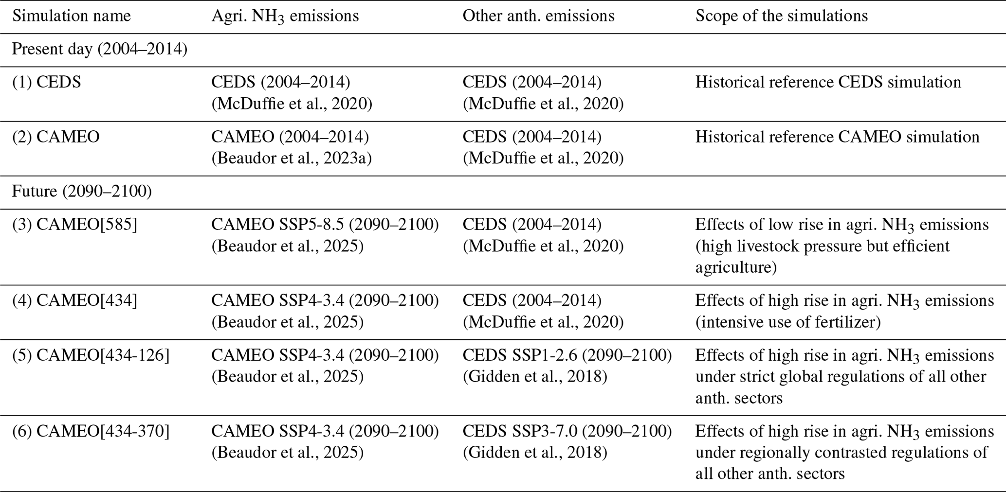
Natural emissions are aggregated to anthropogenic sources in the INCA model. Biogenic surface fluxes of isoprene, terpenes, acetone, and methanol are calculated offline within the ORCHIDEE vegetation model as described by Messina et al. (2016). NH₃ emissions from ocean are taken from Bouwman et al. (1997) and reach 8.2 Tg N yr⁻¹ for the present day, which is higher than the estimate from Paulot et al. (2015) (2–5 Tg N yr⁻¹). Natural emissions of dust and sea salt are computed using the 10 m wind components from the ECMWF reanalysis. For the future simulations (2090–2100), the SSP1-2.6 and SSP3-7.0 anthropogenic emissions (except agricultural sources) provided by Gidden et al. (2018) are used. Natural emissions (except natural soil NH₃ emissions) and biomass burning for gaseous species and particles are kept to their present-day level, even in future simulations, in order to isolate the impact of CAMEO emissions. In total, we performed six simulations, including two present-day simulations, respectively, with CEDS (1) and CAMEO (2) inventories for NH₃ emissions, and four future simulations over 2090–2100, with NH₃ emissions from CAMEO under SSP5.8-5 and SSP4-3.4, by keeping other sources from the present-day levels (3 and 4) and by taking the SSP1-2.6 (low levels; 5) and SSP3-7.0 (regionally contrasted conditions; 6) for other sources. Table 2 summarizes the simulations performed and analyzed in this study.

(McDuffie et al., 2020)(McDuffie et al., 2020)(Beaudor et al., 2023a)(McDuffie et al., 2020)(Beaudor et al., 2025)(McDuffie et al., 2020)(Beaudor et al., 2025)(McDuffie et al., 2020)(Beaudor et al., 2025)(Gidden et al., 2018)(Beaudor et al., 2025)(Gidden et al., 2018)

Table 2 Simulation setup, scope, and corresponding emission datasets. The emission period used is given in parentheses. “Other anth.” accounts for all the species for all the anthropogenic sectors, except NH₃ emitted from the agricultural sector.

4 Present-day atmospheric ammonia, aerosol concentration, and nitrogen deposition fluxes

4.1 Global, regional, and seasonal evaluation with IASI

For over a decade, the IASI instrument has provided measurements of NH₃ at a satisfying spatial resolution and large-scale coverage, which is convenient for modeling evaluation (Van Damme et al., 2014). The simulated monthly distributions of NH₃ are evaluated against observations over 2011–2014 from IASI at the global and regional scale. The IASI data used in this study originate from the IASI instruments on board MetOp-A and MetOp-B, which were launched in 2006 and 2012, respectively. Each instrument overpasses the Earth twice per day, with a footprint of 12 km at the nadir. The instruments cross the Equator in the morning at 09:30 and evening at 21:30 (local solar overpass time). Here we used the IASI NH₃ columns retrieved with version 3 of the Artificial Neural Network for IASI (ANNI) algorithm. An extended description of the retrieval methods and validation works can be found in various publications (Whitburn et al., 2016; Van Damme et al., 2017, 2021; Guo et al., 2021). In the present study, only the morning overpasses have been used as infrared instruments are more sensitive to the lowest layers of the atmosphere at this time of the day (Clarisse et al., 2010). Considering the daily cycle of NH₃ and to be consistent with the satellite observations, the model was run at a 30 min time step and sampled at the corresponding satellite overpass time. Regarding the spatial resolution, the IASI dataset has been gridded on the LMDZ–INCA grid (i.e., resolution of 1.3° in latitude and 2.5° in longitude). The evaluation consists of comparisons of the spatial total NH₃ columns for the two present-day runs (CEDS and CAMEO), along with a seasonal cycle analysis over hotspot regions. Taylor plots and mean bias error scores (MBE; regional mean of the difference between the observation and model) are also presented to assess the spatial and temporal variability in the simulated concentrations compared to the IASI observations considered to be the reference. While IASI observations have already been used for chemical transport model (CTM) evaluations (Heald et al., 2012; Ge et al., 2020; Wang et al., 2021; Vira et al., 2022; Ren et al., 2023), this is the first time that simulated NH₃ columns from LMDZ–INCA are evaluated against spaceborne observations. The Taylor plot approach aims at representing multiple statistical metrics, including the normalized standard deviation, Pearson's R correlation, and a skill function which helps to discriminate the best simulation. The default skill function implemented is defined in Taylor (2001) and decreases toward zero as the correlation becomes more and more negative or as the standard deviation approaches either zero or infinity.

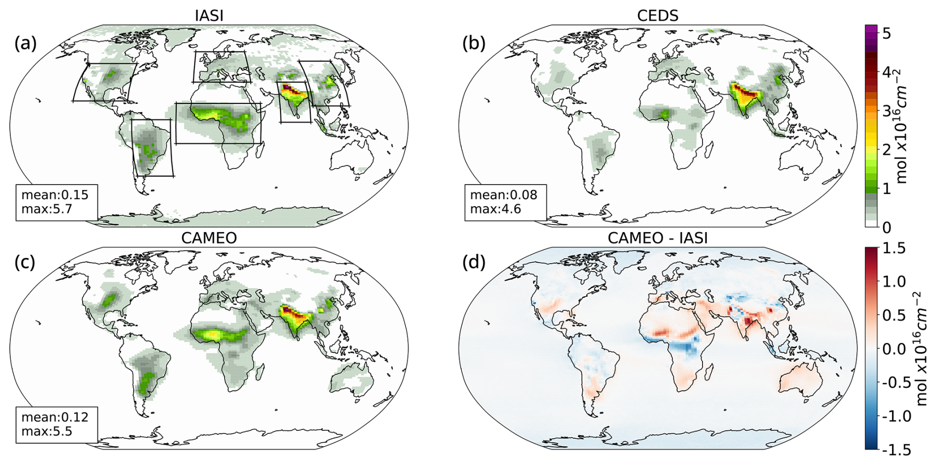
Figure 1 Mean annual NH₃ atmospheric columns observed by the IASI instrument (a) and calculated in the CEDS (b) and CAMEO (c) simulations (2011–2014). The absolute anomalies between the CAMEO and IASI columns are shown in panel (d). The black boxes in panel (a) delimit the regional bounds used in the statistical analysis in the Taylor plots (Fig. 2), the time series analysis (Fig. 3), and the mean bias error calculation in Table 3 ($\text{molec.}\times {\mathrm{10}}^{\mathrm{16}}{\mathrm{cm}}^{-\mathrm{2}}$).

The distributions of the NH₃ columns observed by IASI and computed by LMDZ–INCA with the CEDS or CAMEO NH₃ emissions over 2011–2014 are shown in Fig. 1. The CAMEO simulation captures the NH₃ hotspots over India, equatorial Africa, Latin America, and the US, where the columns are in the range 1–6 $\text{molec.}\times {\mathrm{10}}^{\mathrm{16}}{\mathrm{cm}}^{-\mathrm{2}}$. When the CEDS inventory is replaced by CAMEO in LMDZ–INCA, the global simulated columns are 50 % higher (around 0.04 $\text{molec.}\times {\mathrm{10}}^{\mathrm{16}}{\mathrm{cm}}^{-\mathrm{2}}$) but closer to the IASI-measured global average (0.15 $\text{molec.}\times {\mathrm{10}}^{\mathrm{16}}{\mathrm{cm}}^{-\mathrm{2}}$). The biggest absolute differences are located in northwestern India, where the CAMEO columns are higher by about 2 $\text{molec.}\times {\mathrm{10}}^{\mathrm{16}}{\mathrm{cm}}^{-\mathrm{2}}$. CAMEO emissions also enhance NH₃ columns in China, Latin America, the US, and Africa, especially in the equatorial region when compared to the CEDS simulation. Using CAMEO emissions improved the agreement of LMDZ–INCA with IASI observations in these regions. In particular, the mean bias error (MBE) of the model is reduced from at least 49 % of the observed IASI columns in equatorial Africa and South America when using CAMEO emissions instead of the CEDS inventory (Table 3). The Taylor plots in Fig. 2 represent statistical metrics for temporal and spatial analyses. The temporal analysis is shown for monthly time steps, using triangle markers with T labels, and involves averaging over the corresponding regions. On the other hand, the spatial analysis is derived by averaging over the monthly time series from 2011–2014, indicated by plain circle markers with S labels. These plots include metrics such as the normalized standard deviation (plotted on the x–y axis, where the observation is normalized to 1), Pearson's R correlation, and a skill function, which is represented by grey isolines. The Taylor plots highlight the better performance of the simulated spatial representation of the NH₃ columns in these two regions (equatorial Africa and South America) when CAMEO emissions are prescribed. However, it is important to note potential compensating errors within the regions, particularly in the selected African region (shown in the black box in Fig. 1). For instance, in the Saharan area, CAMEO emissions cause an overestimation of column values by 0.3 $\text{molec.}\times {\mathrm{10}}^{\mathrm{16}}{\mathrm{cm}}^{-\mathrm{2}}$. In contrast, in the tropical sub-Saharan zone, these emissions lead to an underestimation of column values by −0.4 $\text{molec.}\times {\mathrm{10}}^{\mathrm{16}}{\mathrm{cm}}^{-\mathrm{2}}$ (−45 %). This discrepancy might arise from inaccuracies in CAMEO emissions, considering the particular environmental conditions. NH₃ emissions from biomass burning can also be uncertain, and surface–atmosphere exchanges involving fire interactions present in this area are often difficult to consider accurately. Using CAMEO also significantly reduced the modeled bias over the US, with an MBE close to zero (Table 3). It is partially explained by a closer standard deviation to the observations (normalized standard deviation around 1); however, the CEDS simulation seems to be slightly more correlated to IASI (Fig. 2).

Table 3 Regional spatial mean bias error (MBE) NH₃ columns from the CEDS and CAMEO simulations ($\text{molec.}\times {\mathrm{10}}^{\mathrm{16}}{\mathrm{cm}}^{-\mathrm{2}}$). The biases are computed using IASI observations over the 2011–2014 period. The numbers of pixels within the regions over which the average has been computed are given in parentheses for each region.

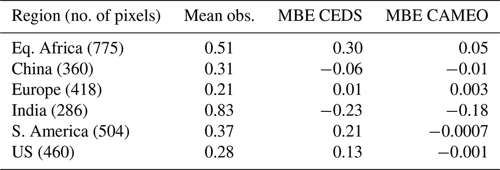
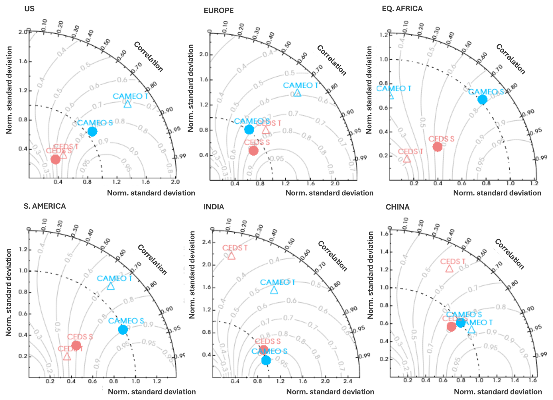
Figure 2 Regional Taylor plots for the simulated atmospheric NH₃ columns from the CAMEO and CEDS simulations evaluated with IASI observations. The plots include temporal statistic metrics at the monthly time step (first averaged in space over the corresponding regions with triangle markers and T labels) and spatial statistic metrics (first averaged in time over monthly time series of the 2011–2014 period, plain circles markers, and S labels), including the normalized standard deviation (presented on the x–y axis; observation =1), Pearson's R correlation, and a skill function (grey isolines). It is important to note that each region has been chosen carefully with a sufficient number of pixels as given in Table 3. The plots have been performed using the CDAT library in Python, according to Taylor (2001).

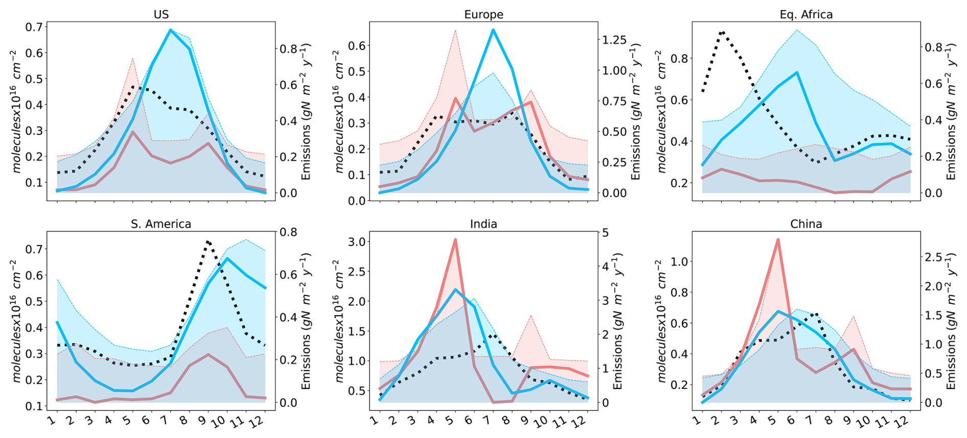
Figure 3 Regional mean seasonal cycle (2011–2014) of NH₃ atmospheric columns observed by the IASI satellite (dotted black lines) and calculated in the CEDS (pink lines) and CAMEO (blue lines) simulations ($\text{molec.}\times {\mathrm{10}}^{\mathrm{16}}{\mathrm{cm}}^{-\mathrm{2}}$). Regional total NH₃ emissions from CEDS and CAMEO are shown with the shaded areas. Emissions also include biomass burning from GFED v4s and other anthropogenic emissions from CEDS for consistency with the simulated columns ($\mathrm{g}\mathrm{N}{\mathrm{m}}^{-\mathrm{2}}{\mathrm{yr}}^{-\mathrm{1}}$).

On the western coast of Africa, the CAMEO emissions also lead to an improvement, where the resulting columns over the Atlantic Ocean depict the same pattern as IASI. It is explained by higher agricultural emissions and the addition of natural soil emissions calculated by CAMEO, which are missing in CEDS (see Fig. S2). In India, both model simulations result in a normalized standard deviation close to 1 for the spatial distributions. The correlations are high ($\left|r\right|>\mathrm{0.8}$), but the spatial patterns correlate better with IASI when using CAMEO. Over India, even though the bias is slightly reduced in CAMEO, the model overestimates the columns with a remaining high bias ($\sim -\mathrm{0.18}\text{molec.}\times {\mathrm{10}}^{\mathrm{16}}{\mathrm{cm}}^{-\mathrm{2}}$).

The mean seasonal cycle over 2011–2014 is also analyzed for several regions (Fig. 3). The seasonal cycle of the two simulated NH₃ columns correlates with the emission's temporal evolution (not shown). The seasonal variations in NH₃ columns in the CEDS simulation highlight two peaks in April and September for most regions, reflecting the artificial seasonal profile used in the inventory. In CAMEO, the seasonality varies according to the region. In the US and Europe, the CAMEO columns show a unique peak (0.7 $\text{molec.}\times {\mathrm{10}}^{\mathrm{16}}{\mathrm{cm}}^{-\mathrm{2}}$) during summer, while the IASI observations inform about a lower maximum value (0.5 and 0.4 $\text{molec.}\times {\mathrm{10}}^{\mathrm{16}}{\mathrm{cm}}^{-\mathrm{2}}$, respectively) reached over March–September. In Europe, CEDS surpasses CAMEO when it comes to the magnitude of seasonal variations. In equatorial Africa, South America, India, and China, CAMEO shows good agreement with the IASI columns, and the seasonal cycles are very close, with values in the same ranges. CAMEO emissions improve the representation of the atmospheric columns, especially in South America and equatorial Africa, where the columns in CEDS are at least 2 times lower compared to IASI. In Africa, the temporal variability is more accurately simulated with CAMEO with a higher skill function in the Taylor plot, even though the correlation is reduced (Fig. 2). Over South America, the improvement is even stronger where the skill function gained two units. In India, CAMEO and CEDS simulate a peak value occurring 2 months earlier than that measured by IASI, but the value is 1.5 times higher with CEDS than with CAMEO. CAMEO depicts a better seasonal amplitude with a 2-month peak starting in May and lasting until June, closer to the observations leading to a better model performance (Fig. 2).

4.2 Regional comparison with worldwide ground-based networks

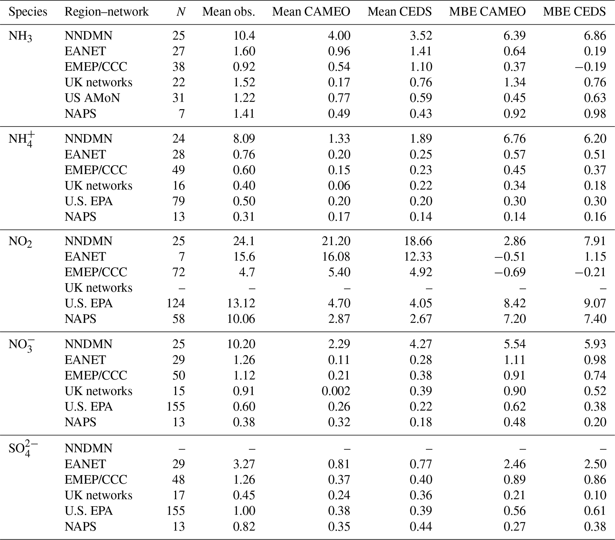
In total, 10 monitoring networks of surface NH₃, ${\mathrm{NH}}_{\mathrm{4}}^{+}$, NO₂, ${\mathrm{NO}}_{\mathrm{3}}^{-}$, and ${\mathrm{SO}}_{\mathrm{4}}^{\mathrm{2}-}$ concentrations from East Asia, North America, and Europe have been exploited to extend our evaluation beyond the NH₃ columns. The simulated surface concentrations for 2015 have been compared yearly with the data observed from 2015 by extracting the closest pixel from the LMDZ–INCA simulation for each site. As recommended in Ge et al. (2021), we only consider measurements where 75 % of the year was captured to avoid bias in our analysis, and we perform yearly averages on the model data. In this study, we utilize data from the Chinese Nationwide Nitrogen Deposition Monitoring Network (NNDMN from Xu et al., 2019), the acid deposition monitoring network in East Asia and Southeast Asia (EANET; 13 countries; https://www.eanet.asia/, last access: 12 February 2025), the UK Acid Gases and Aerosol Monitoring Network (AGANet; 30 sites; https://uk-air.defra.gov.uk/networks/network-info?view=aganet, last access: 12 February 2025), the European Monitoring and Evaluation Programme/Chemical Coordinating Centre (EMEP/CCC; https://ebas-data.nilu.no/default.aspx, last access: 12 February 2025), the U.S. Environmental Protection Agency (EPA; https://www.epa.gov/outdoor-air-quality-data, last access: 12 February 2025), the Ammonia Monitoring Network (AMoN; https://nadp.slh.wisc.edu/sites/amon-ab35/, last access: 12 February 2025), and the National Air Pollution Surveillance (NAPS; https://www.canada.ca/en/services/environment/weather/airquality.html, last access: 12 February 2025) program. Main statistic scores are given in Table 4, comparing observations with CAMEO and CEDS runs. Scatter plots of the annual mean modeled in CAMEO and measured surface concentrations, along with Pearson's coefficients, are given for each regional network in Figs. S4–S6. Analog plots for the CEDS simulation are given in Figs. S7–S9. An evaluation for 2010 has also been conducted to enhance the robustness of our findings, and similar regional signals are found as for 2015. Owing to the fewer observations available globally in 2010 compared to 2015, these results are presented in Figs. S10–S12. Overall, surface NH₃, ${\mathrm{NH}}_{\mathrm{4}}^{+}$, NO₂, ${\mathrm{NO}}_{\mathrm{3}}^{-}$, and ${\mathrm{SO}}_{\mathrm{4}}^{\mathrm{2}-}$ concentrations simulated by LMDZ–INCA are well correlated to the observations worldwide (R_T>0.5). However, simulated concentrations are underestimated for most species, especially in China, where observed concentrations are by far the highest, with, for example, an estimated MBE for NH₃ concentrations at 6.0 µg m⁻³ (annual observed average at 10.4 µg m⁻³; Table 4). This positive bias seems to be due to an underestimation in the hotspot region of Beijing but also in more remote areas, where differences can reach 15.5 µg m⁻³ (Fig. S4f). The IASI instrument does not necessarily detect the highest columns in these regions (Fig. 1). For most networks, prescribing CAMEO highlights reductions in the bias compared to CEDS (−15 % for AMoN in the US and around −4.5 % for NNDMN and NAPS). In North America, CAMEO reflects a realistic spatial pattern against measurements with high concentrations of NH₃ located in the Midwest region of the US ($>\mathrm{4}\mathrm{\mu }\mathrm{g}{\mathrm{m}}^{-\mathrm{3}}$) and rather low concentrations on the Mid-Atlantic side. An underestimation of CAMEO is still observable in the northeast region of the Midwest ($<\mathrm{2}\mathrm{\mu }\mathrm{g}{\mathrm{m}}^{-\mathrm{3}}$; Fig. S6f). Even though the spatial gradient is fairly represented in the model, it is crucial to note that only a few observations are available, especially in the mid-US region. This intensive agricultural area would benefit from further observation data for a more accurate evaluation. CAMEO emissions do not improve the NH₃ concentration representations measured in the EANET and European networks.

It is worth pointing out that the model–observation comparison highlights an underestimation of the simulated ammonium–nitrate concentrations at the surface (Figs. S4–S12b and d). A combination of factors explains the low simulated nitrate concentrations at the surface. This version of the model has always shown a strong vertical transport combined with low scavenging in the upper troposphere (Bian et al., 2017). To some extent, this strong transport of nitrates to the upper troposphere is a robust signal and has been observed in the Asian tropopause aerosol layer region during the monsoon season (June–July–August) (Höpfner et al., 2019; Yu et al., 2022). However, the CAMEO NH₃ emissions are significantly increased compared to CEDS during this period over India; more nitrates are produced and subsequently transported to the upper troposphere (UT) in that region and then spread all over the globe due to the high residence time of aerosols in the UT. This feature of the scavenging is currently investigated in a newer version (79 levels; CMIP6 physics) of the model.

Table 4 Summary statistics of model comparison (CAMEO and CEDS runs) with measurements for 2015 in East Asia and Southeast Asia (NNDMN and EANET networks), Europe and UK (EMEP/CCC; UK networks), North America (U.S. EPA, AMoN, and NAPS). N represents the number of measuring sites. Annual average concentrations and mean bias error (MBE) are given in µg m⁻³.

The main takeaway from the evaluation of NH₃ columns and surface concentrations is that using CAMEO emissions results in a significant improvement in the spatial and temporal patterns, particularly in the seasonal cycle, compared to CEDS, except in the US and Europe. It is still important to note that CAMEO improves the ground spatial variability in NH₃ in the US as highlighted by measurement comparisons. The skill functions shown in the Taylor plots indicate that CAMEO emissions can more accurately capture the temporal variability in emissions in hotspot regions when compared to IASI observations. It is important to focus on matching seasonal cycles rather than only comparing annual averages for multiple reasons. Seasonal cycles provide insights into the variations in emissions and atmospheric pathways throughout the year, which can be linked to meteorological conditions (air temperature and precipitation), seasonal activities (like fertilizer application or manure handling), and specific events (like biomass burning). Understanding these patterns allows for more accurate predictions of air pollution and climate impacts. The effort to improve emission estimates, particularly in regions where discrepancies exist, such as Europe and the US, highlights the importance of utilizing process-based approaches that allows room for considering the bi-directional property of ammonia.

4.3 Surface nitrogen deposition intercomparison

In this section, we present an analysis of the total (dry + wet) annual deposition of NH_x ($={\mathrm{NH}}_{\mathrm{3}}+{\mathrm{NH}}_{\mathrm{4}}^{+}$) and NO_y ($=\mathrm{NO}+{\mathrm{NO}}_{\mathrm{2}}+{\mathrm{NO}}_{\mathrm{3}}+{\mathrm{HNO}}_{\mathrm{2}}+{\mathrm{HNO}}_{\mathrm{3}}+{\mathrm{HNO}}_{\mathrm{4}}+\mathrm{2}{\mathrm{N}}_{\mathrm{2}}{\mathrm{O}}_{\mathrm{5}}+\text{PAN}+\text{organic nitrates}+\text{particulate}{\mathrm{NO}}_{\mathrm{3}}^{-}$).

The simulated deposition fluxes (CEDS and CAMEO) are also compared against two model-based estimates, with one used in the most recent Coupled Model Intercomparison Project (CMIP) exercise (IGAC/SPARC Chemistry–Climate Model Initiative; CCMI hereafter; Eyring et al., 2013) and the other using EMEP MSC–W (European Monitoring and Evaluation Programme Meteorological Synthesizing Centre–West) from Ge et al. (2022). N deposition fluxes from CCMI are commonly used as forcing files in the LSM, as in the ORCHIDEE model. CCMI deposition fields are available globally at a resolution of 0.5°×0.5° from 1860 to 2014. In the CCMI models, nitrogen emissions from natural biogenic sources, lightning, anthropogenic sources, and biomass burning are taken from CMIP5 exercise (Lamarque et al., 2010). Regarding N deposition from Ge et al. (2022), the CTM EMEP MSC–W has been used to simulate dry and wet deposition fluxes of N_r species for 2015. In their configuration, meteorology comes from the Weather Research and Forecast model (WRF; Simpson et al., 2012). The N anthropogenic emissions used were derived from the V6 ECLIPSE inventory (https://iiasa.ac.at/web/home/research/researchPrograms/air/ECLIPSEv6.html, last access: 20 May 2021) for 2015 with monthly profiles deduced from the EDGAR time series (Crippa et al., 2020), according to Ge et al. (2021). NO_x and volatile organic compound emissions from the forest, vegetation fires, lightning, and soil were also included.

As CCMI fluxes are only available until 2014 and files from Ge et al. (2022) are provided for 2015 only, a 2010–2014 climatology has been calculated for CCMI-, CAMEO-, and CEDS-simulated N depositions. Ge et al. (2022) do not provide monthly fields; thus, only CCMI, CAMEO and CEDS time series for the same 2010–2014 climatology have been further explored for the seasonality analysis.

Global Nr (reactive nitrogen) deposition was estimated at 108 and 127 Tg N yr⁻¹ over 2010–2014 in the CEDS and CAMEO simulations (land is ∼80 %; ocean is ∼20 %). CEDS compares well with the 102 and 114 Tg N yr⁻¹ estimated from CCMI and Ge et al. (2022), but CAMEO is closer to the 119 Tg N yr⁻¹ quantified for 2010 from the recent study from Liu et al. (2022). The ratio of NH_x to total N_r depositions between CCMI, CEDS, and CAMEO shows a good agreement; however, EMEP MSC–W depicts a much less important contribution of NH_x to the total N_r depositions all over the world.

4.3.1 Reduced nitrogen deposition

Global surface NH_x depositions reach 65 Tg N yr⁻¹, with CAMEO showing a good agreement between CCMI, CEDS, and EMEP MSC–W and CAMEO appearing as the highest estimate (Fig. 4). This difference between CAMEO and the other estimates is partly explained by the high values over Africa (Fig. 5) with a total budget of 14 Tg N yr⁻¹, which is twice the one estimated in CCMI, CEDS, and EMEP MSC–W but also to a smaller extent by higher budgets in Oceania and Latin America. Higher [NH₃] due to enhanced NH₃ emissions in CAMEO explains these regional patterns, together with no enhanced aerosol (${\mathrm{NH}}_{\mathrm{4}}^{+}$, ${\mathrm{NO}}_{\mathrm{3}}^{-}$, and ${\mathrm{SO}}_{\mathrm{4}}^{\mathrm{2}-}$) formation because of the low NO_x conditions (Figs. 6 and 7). It means that even though there is more NH₃, it remains in its gaseous phase, and the deposition pathway is favored in these regions when CAMEO emissions are used. As mentioned previously, Vira et al. (2020) estimated high agricultural NH₃ emissions over Africa with the FAN v2 model when compared to the literature. In a recent evaluation work using observations from INDAAF (International Network to study Deposition and Atmospheric composition in Africa), they show an overestimation of their NH_x wet deposition flux of around 10 % (Vira et al., 2022). We also compared our simulated NH_x wet deposition fluxes from two grid cells corresponding to stations from INDAAF situated in western Africa (see Fig. S13 for the exact locations). The CAMEO simulation compares much better than CEDS to the observed ${\mathrm{NH}}_{\mathrm{4}}^{+}$ wet deposition, especially at the Katibougou station, where a clear seasonal cycle with a similar peak in summer is represented (see Fig. S14).

Figure 4 Global and regional annual NH_x and NO_y deposition in Tg N yr⁻¹ from CCMI for 2010–2014, from CEDS and CAMEO simulations for 2010–2014, and from EMEP MSC–W (Ge et al., 2022) for 2015. Note that the global budget accounts for continents and oceans. China–K–J accounts for China–Korea–Japan.

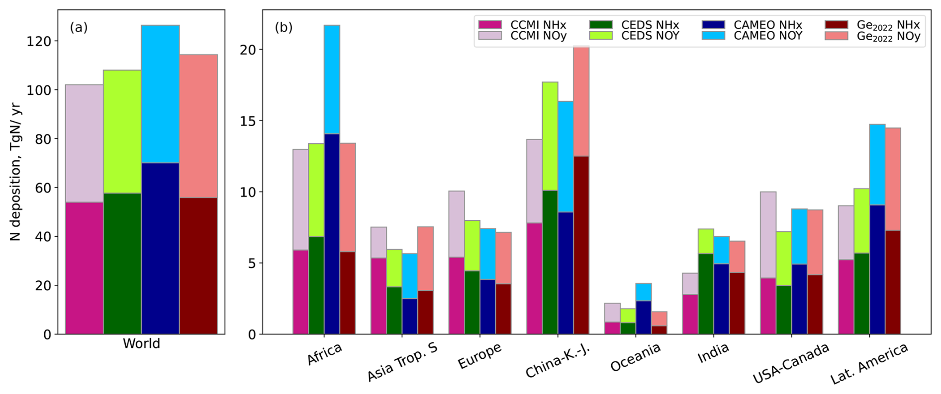
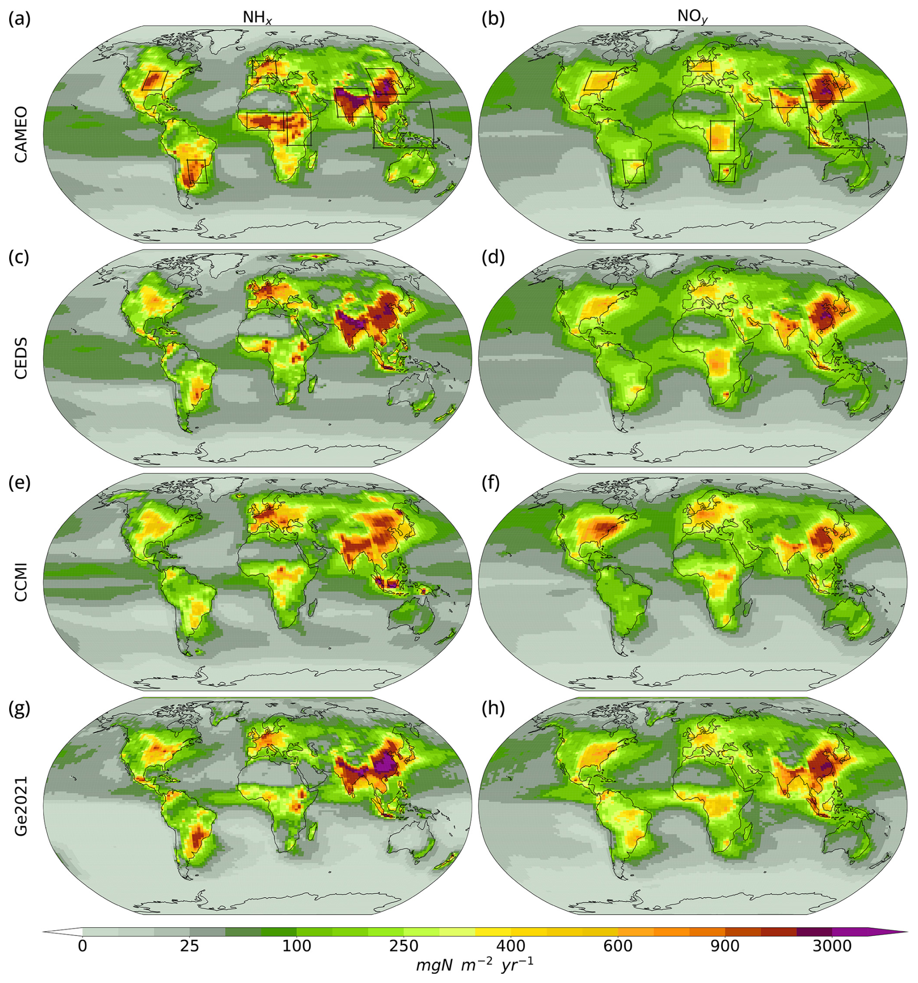
Figure 5 Annual mean total (dry + wet) NH_x (first column) and NO_y (second column) deposition for present-day conditions. The first row shows the N-deposition fluxes calculated from the most recent CMIP exercise (IGAC/SPARC Chemistry–Climate Model Initiative, CCMI; Eyring et al., 2013; 2010–2014 climatology); the second and third rows correspond to LMDZ–INCA simulations, where CEDS and CAMEO emissions are prescribed, respectively (2010–2014 climatology); and the last row displays recent modeling results from Ge et al. (2022) using the EMEP model (2015). The black boxes in panels (a) and (b) delimit the regional bounds for the seasonal variability analysis ($\mathrm{mg}\mathrm{N}{\mathrm{m}}^{-\mathrm{2}}{\mathrm{yr}}^{-\mathrm{1}}$).

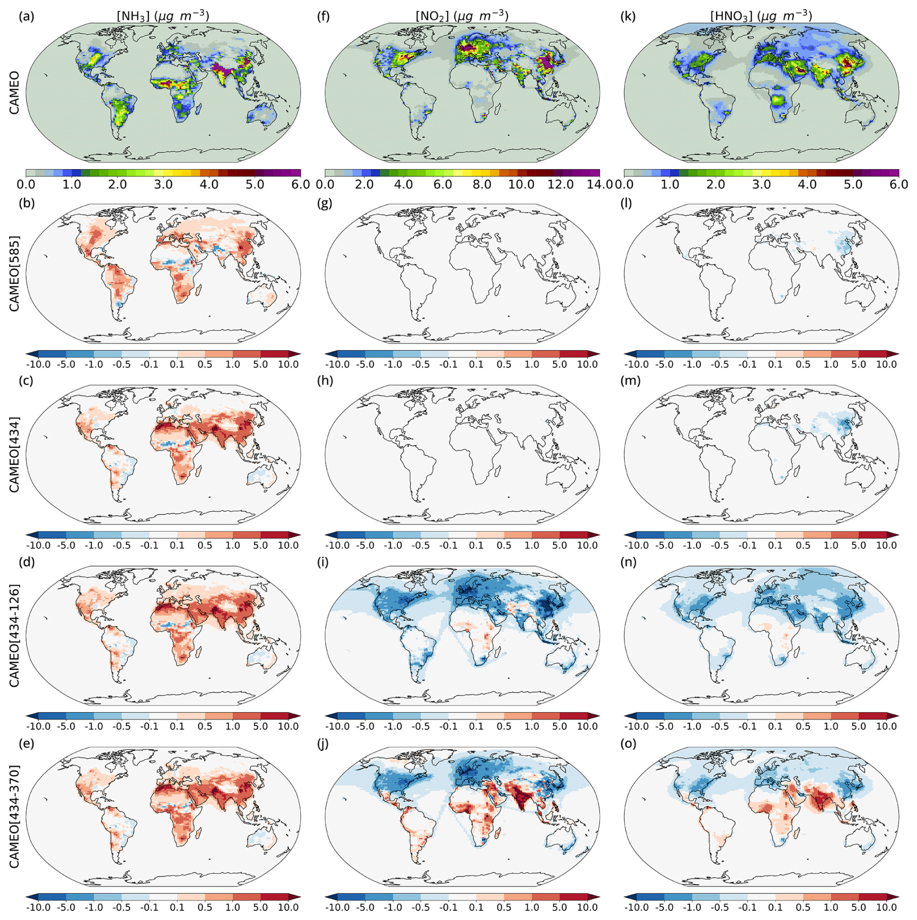
Figure 6 Mean annual surface concentrations of NH₃, NO₂, and HNO₃ simulated in the CAMEO simulation (first row; over 2004–2014) and the anomalies between the CAMEO[SSPi] and CAMEO simulations ([SSPi] is 585, 434, 434-126, and 434-370 in rows 2–5; over 2090–2100) (µg m⁻³).

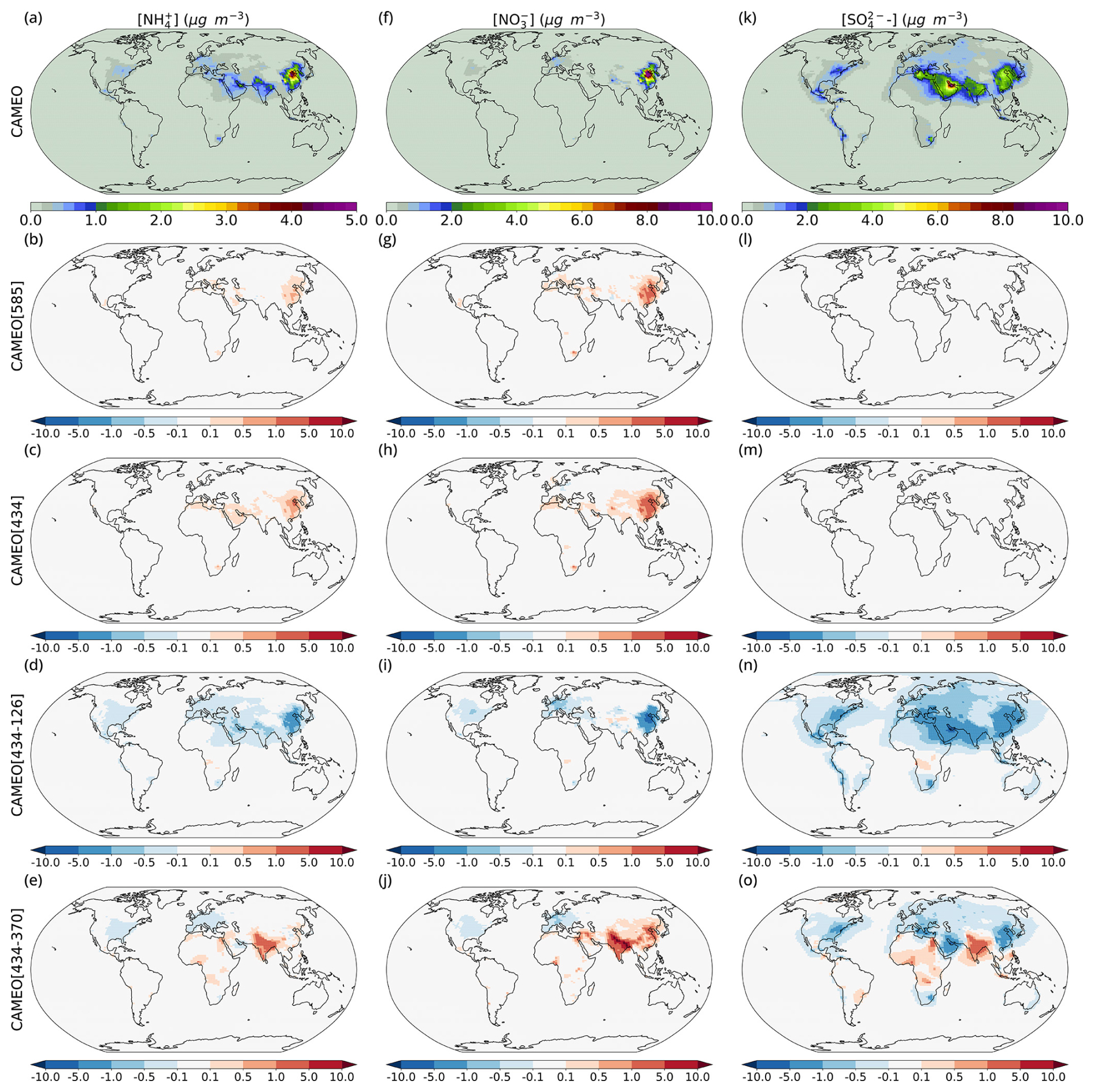
Figure 7 Mean annual surface concentrations of ${\mathrm{NH}}_{\mathrm{4}}^{+}$, ${\mathrm{NO}}_{\mathrm{3}}^{-}$, and ${\mathrm{SO}}_{\mathrm{4}}^{\mathrm{2}-}$ simulated in the CAMEO simulation (first row; over 2004–2014) and the anomalies between the CAMEO[SSPi] and CAMEO simulations ([SSPi] is 585, 434, 434-126, and 434-370 in rows 2–5; over 2090–2100) (µg m⁻³).

Regarding the other regions, NH_x deposition from LMDZ–INCA (CEDS and CAMEO) and EMEP MSC–W reaches values up to 3000 $\mathrm{mg}\mathrm{N}{\mathrm{m}}^{-\mathrm{2}}{\mathrm{yr}}^{-\mathrm{1}}$ in India and China, while CCMI fluxes do not exceed 1900 $\mathrm{mg}\mathrm{N}{\mathrm{m}}^{-\mathrm{2}}{\mathrm{yr}}^{-\mathrm{1}}$ (Fig. 5). Same patterns are observable over central Africa, Latin America, and the US, where CCMI NH_x deposition (maximum between 500 and 1000 $\mathrm{mg}\mathrm{N}{\mathrm{m}}^{-\mathrm{2}}{\mathrm{yr}}^{-\mathrm{1}}$) is lower than the LMDZ–INCA and EMEP MSC–W deposition rates (maximum between 800 and 1900 $\mathrm{mg}\mathrm{N}{\mathrm{m}}^{-\mathrm{2}}{\mathrm{yr}}^{-\mathrm{1}}$). Over these regions, the CAMEO simulation depicts much higher-deposition fluxes, which are explained by higher emissions prescribed in this run than in CEDS (see Fig. S2). However, in southeastern Asia, the CCMI deposition reaches 7000 $\mathrm{mg}\mathrm{N}{\mathrm{m}}^{-\mathrm{2}}{\mathrm{yr}}^{-\mathrm{1}}$, while in LMDZ–INCA and EMEP MSC–W the maximum value is around 1400 $\mathrm{mg}\mathrm{N}{\mathrm{m}}^{-\mathrm{2}}{\mathrm{yr}}^{-\mathrm{1}}$.

There are important disagreements in the NH_x deposition seasonal cycle between LMDZ–INCA simulations and CCMI in almost all the regions (see Fig. S15). CEDS NH_x deposition variations are well correlated with the NH₃ variations in the CEDS emission inventory used as forcing file for the flux calculation in the model. NH₃ emissions from the CEDS inventory describe two peaks, namely an important one in May and another smaller in September, which are clearly observable in the CEDS depositions. CAMEO NH_x depositions describe a pattern that differs from one region to another but with a peak in summer for most regions. The summer peak is also reflected in the emission seasonality as analyzed in Beaudor et al. (2023a). Both dry and wet NH_x depositions from LMDZ–INCA have the same seasonal cycle, except in east Africa, India, and Latin America, where, in these regions, wet deposition is largely dominant. Aside from these regions, wet and dry depositions have similar contributions to the total depositions. In their study, Ge et al. (2022) found a higher contribution of dry deposition in almost all the continental regions. In the CCMI depositions, except for Southeast Asia, variations over the year are weak, with no clear seasonal pattern.

It is worth pointing out that in the LMDZ–INCA model no pH adjustment is considered for the NH₃ Henry's law constant, while it appears to be important in controlling the wet NH₃ deposition. Bian et al. (2017) investigated the impact of the pH-dependent NH₃ wet deposition on atmospheric NH₃ and associated nitrogen species with the global modeling initiative (GMI) and found that, without pH correction, the NH₃ wet deposition decreases significantly (from 17.5 to 1.1 Tg N yr⁻¹). Because NH₃ deposition has an impact on its atmospheric lifetime and, therefore, is an important factor in the ammonium–nitrate system, it would also be interesting to evaluate the sensitivity of the effective NH₃ Henry's law constant and the consideration of the pH correction in LMDZ–INCA.

4.3.2 Nitrogen oxide deposition

NO_y deposition patterns over Africa, India, and China are consistent between the four estimates, especially for the CEDS and CAMEO simulations and EMEP MSC–W (Fig. 5). There are no major differences between CEDS and CAMEO simulated NO_y deposition fluxes since NH₃ emissions have only a small impact on nitrate deposition. However, CCMI fluxes in the US and Europe (1300 and 900 $\mathrm{mg}\mathrm{N}{\mathrm{m}}^{-\mathrm{2}}{\mathrm{yr}}^{-\mathrm{1}}$) are more important than LMDZ–INCA (600 and 500 $\mathrm{mg}\mathrm{N}{\mathrm{m}}^{-\mathrm{2}}{\mathrm{yr}}^{-\mathrm{1}}$) and EMEP MSC–W (900 and 700 $\mathrm{mg}\mathrm{N}{\mathrm{m}}^{-\mathrm{2}}{\mathrm{yr}}^{-\mathrm{1}}$) depositions. On the opposite side, in Latin America, CCMI depositions are the lowest. Global NO_y deposition budgets from CCMI and LMDZ–INCA vary between 39 and 43 Tg N yr⁻¹, while the EMEP MSC–W estimate is 47 Tg N yr⁻¹ (Fig. 4). Similarly, for NH_x, China, Africa, and Latin America are the most important contributors to the global NO_y deposition budget in EMEP MSC–W and LMDZ–INCA estimates (about 47 %). CCMI estimates higher NO_y depositions in North America than in Latin America. The three regions Africa, North America, and China account for half of the CCMI budget.

CCMI and LMDZ–INCA seasonal cycles of NO_y deposition are very well correlated (see Fig. S16). Contrary to NH_x, which are primarily driven by only a few sources of emissions (mainly agricultural NH₃), NO_y are the results of NO_x sources and reactions involving several nitrate species. However, NO_x emissions mainly come from the energy, transportation, and industrial sectors (Hoesly et al., 2018; McDuffie et al., 2020), whose seasonal cycles are better known than the agricultural one. Similarly, for NH_x, NO_y wet fluxes are contributing the most to the total depositions in most regions, except in southern Africa, Europe, and India, where dry deposition dominates during several months. The main differences between CEDS and CAMEO are observed in the wet deposition in winter in Latin America and in southern Africa but also in India in summer and the whole year in southern–eastern Asia. It indicates that NH₃ emissions rather impact wet NO_y deposition fluxes mostly when a direct loss through scavenging occurs, such as during the monsoon season in India.

5 Impact of future emissions

5.1 Impact on atmospheric composition

Considering future CAMEO emissions under SSP5-8.5 and SSP4-3.4 in LMDZ–INCA highlights the range of the possible impact of future NH₃ emissions on N species and aerosol. Both scenarios of emissions lead to a global increase in the N species and aerosol burdens, which also vary according to the NO_x and SO₂ emission trends (Table 5).

Table 5 Tropospheric burden and deposition losses (Tg N yr⁻¹) of ammonia (NH₃), ammonium particles (${\mathrm{NH}}_{\mathrm{4}}^{+}$), nitric acid (HNO₃), and fine nitrate particles (${\mathrm{NO}}_{\mathrm{3}}^{-}$) for present-day (2004–2014) and future (2090–2100) simulations. N₂O production through the NH₃ gas phase loss (Tg N yr⁻¹) is also included. Please note that total emissions include biomass burning (4.2 Tg N yr⁻¹).

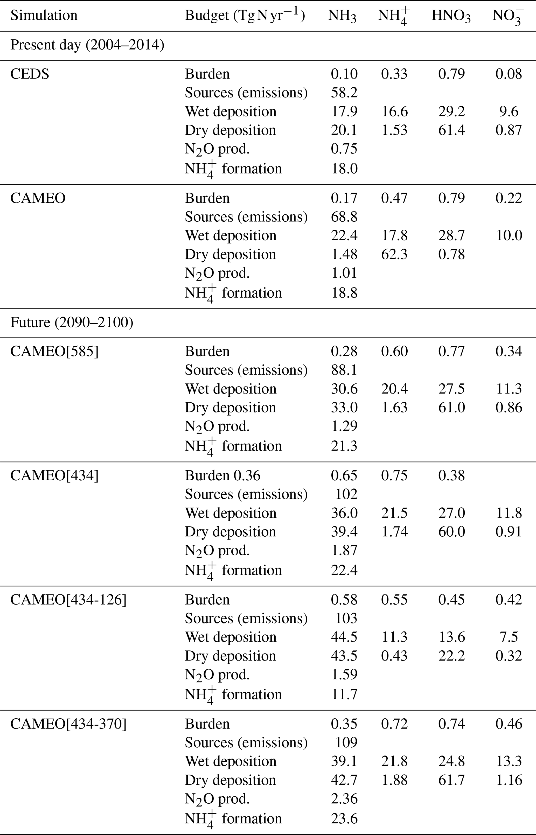
Relative to the present-day level with CAMEO, NH₃ burdens are increased by 59 % in CAMEO[585], 111 % in both CAMEO[434] and CAMEO[434-370], and by 235 % in CAMEO[434-126] which is considered the “higher” scenario regarding NO_x and SO₂ emissions. In CAMEO[434-126], the burden of ${\mathrm{NH}}_{\mathrm{4}}^{+}$ (0.55 Tg N yr⁻¹) is similar to the value of NH₃ (0.58 Tg N yr⁻¹), while in CAMEO[434] and CAMEO[434-370], the ${\mathrm{NH}}_{\mathrm{4}}^{+}$ burden ($\sim \mathrm{0.72}\mathrm{Tg}\mathrm{N}{\mathrm{yr}}^{-\mathrm{1}}$) is about twice that of NH₃. Regarding the HNO₃ burden, it is similar to the present-day value in CAMEO[434] and CAMEO[434-370] ($\sim \mathrm{0.74}\mathrm{Tg}\mathrm{N}{\mathrm{yr}}^{-\mathrm{1}}$) but much smaller in CAMEO[434-126] (Table 5). It is explained by the lower NO_x emissions used in the later simulation compared to the other simulations (9.2 against 39 Tg N yr⁻¹) (see Table 1). However, the ${\mathrm{NO}}_{\mathrm{3}}^{-}$ burden is within the same range of values for the three future simulations (0.34–0.45 Tg N yr⁻¹), which can be twice as high as in the historical CAMEO run.

The impact of future CAMEO emissions under SSP4-3.4 on the distributions of NH₃, NO₂, and HNO₃ surface concentrations are presented in Fig. 6. Compared to the historical CAMEO simulation, all of CAMEO[SSP4-3.4-i] depicts large increases in [NH₃] of about 5–10 µg m⁻³ (>100 %) over northern Africa, northern India, and eastern China (Fig. 6c–e), corresponding to the regions experiencing the most important increases in the agricultural NH₃ emissions ($>\mathrm{4}\mathrm{g}\mathrm{N}{\mathrm{m}}^{-\mathrm{2}}{\mathrm{yr}}^{-\mathrm{1}}$; see Fig. S2). As only negligible differences in the other future anthropogenic NH₃ emissions are notable, the impact of the CAMEO[SSP4-3.4] emissions on [NH₃] is similar for the three simulations. The impact on [NO₂] and [HNO₃] is much more contrasted between the simulations. In CAMEO[434], as the NO_x emissions are kept at their present-day level, no impact is observable. However, in CAMEO[434-126] and CAMEO[434-370], the NO_x emissions vary from the historical levels; in CAMEO[434-126], the emissions are much lower all over the globe, while in CAMEO[434-370], emissions are largely reduced in the most developed countries (Europe, China, and the US) and increased in the Southern Hemisphere, along with India and the Gulf states. It leads to a decrease from around 60 % to 80 % (5 to 12 µg m⁻³) in [NO₂] and (1 to 3 µg m⁻³) in [HNO₃] over China, Europe, and the US in CAMEO[434-126] (Fig. 6i and n). In CAMEO[434-370], the impact of the future emissions on [NO₂] and [HNO₃] also follows NO_x emission trends, with the most important increases located in India (15 and 8 µg m⁻³, respectively) and smaller decrease situated in Europe, China, and the US (Fig. 6j and o).

As a result of these changes in nitrate precursor surface concentrations, nitrate and sulfate particles are expected to vary significantly in the future. In order to understand future patterns in the nitrate and sulfate aerosol formations, the state of ammonia neutralization of the sulfuric and nitric acids is shown for different pressure levels in Fig. 8.

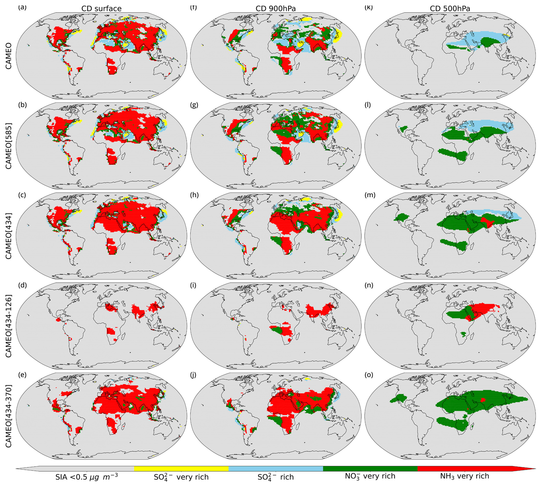
Figure 8 The state of the ammonia neutralization of sulfuric and nitric acids for areas where the secondary inorganic aerosol concentration in the fine particle fraction (PM_2.5) is $>\mathrm{0.5}\mathrm{\mu }\mathrm{g}{\mathrm{m}}^{-\mathrm{3}}$, calculated from the different simulations (averages done over 2004–2014 for CAMEO and over 2090–2100 for CAMEO[SSPi]) at the surface, and 900 and 500 hPa (first, second, and third columns). The four chemical domains are defined as very sulfate-rich ($T_{\mathrm{A}}/T_{\mathrm{S}}<\mathrm{1}$; yellow areas), sulfate-rich ($\mathrm{1}<T_{\mathrm{A}}/T_{\mathrm{S}}<\mathrm{2}$; blue areas), nitrate-rich ($\mathrm{0}<T_{\text{A-free}}/T_{\mathrm{N}}<\mathrm{1}$; green areas), and ammonia-rich ($T_{\text{A-free}}/T_{\mathrm{N}}>\mathrm{1}$; red areas).

Four chemical domains can be derived from the simulated relative abundances of NH₃, ${\mathrm{NH}}_{\mathrm{4}}^{+}$, ${\mathrm{NO}}_{\mathrm{3}}^{-}$, HNO₃, and ${\mathrm{SO}}_{\mathrm{4}}^{\mathrm{2}-}$ (Metzger et al., 2002; Xu and Penner, 2012; Hauglustaine et al., 2014; Paulot et al., 2016; Ge et al., 2022). To gain a better understanding of the behavior of ammonia and its persistence in the atmosphere under future scenarios, we have selected different pressure levels, including the surface level, 900, and 500 hPa. First, we define the total molar concentrations of sulfate (T_S, including all forms of ${\mathrm{SO}}_{\mathrm{4}}^{\mathrm{2}-}$ as H₂SO₄, NH₄HSO₄, (NH₄)₃H(SO₄)₂, and (NH₄)2), nitrate (T_N), ammonia (T_A), and the ammonia needed to fully neutralize the sulfate (T_A-free).

$$\begin{array}{}\text{(2)}& {\displaystyle }& {\displaystyle }{T}_{\mathrm{S}}=\left[{\mathrm{SO}}_{\mathrm{4}}^{\mathrm{2}-}\right],\text{(3)}& {\displaystyle }& {\displaystyle }{T}_{\mathrm{N}}=\left[{\mathrm{NO}}_{\mathrm{3}}^{-}\right]+\left[{\mathrm{HNO}}_{\mathrm{3}}\right],\text{(4)}& {\displaystyle }& {\displaystyle }{T}_{\mathrm{A}}=\left[{\mathrm{NH}}_{\mathrm{3}}\right]+\left[{\mathrm{NH}}_{\mathrm{4}}^{+}\right],\text{(5)}& {\displaystyle }& {\displaystyle }{T}_{\text{A-free}}=T_{\mathrm{A}}-\mathrm{2}\times T_{\mathrm{s}}.\end{array}$$

The four chemical domains are defined as very sulfate-rich ($T_{\mathrm{A}}/T_{\mathrm{S}}<\mathrm{1}$), sulfate-rich ($\mathrm{1}<T_{\mathrm{A}}/T_{\mathrm{S}}<\mathrm{2}$), nitrate-rich ($\mathrm{0}<T_{\text{A-free}}/T_{\mathrm{N}}<\mathrm{1}$), and ammonia-rich ($T_{\text{A-free}}/T_{\mathrm{N}}>\mathrm{1}$). When $T_{\text{A-free}}/T_{\mathrm{N}}>\mathrm{1}$, sufficient ammonia remains to react with nitrate to form NH₄NO₃. The resulting calculated domains are illustrated in Fig. 8. In order to focus on the most important anthropogenic sources, we imposed a threshold on the secondary inorganic aerosol (SIA) concentration, which is set as (${\mathrm{NH}}_{\mathrm{4}}^{+}$ + ${\mathrm{NO}}_{\mathrm{3}}^{-}$ + ${\mathrm{SO}}_{\mathrm{4}}^{\mathrm{2}-}$) $\ge \mathrm{0.5}\mathrm{\mu }\mathrm{g}{\mathrm{m}}^{-\mathrm{3}}$. This threshold has been arbitrarily chosen, similar to that seen in Ge et al. (2022). In the rich and very rich domains ${\mathrm{SO}}_{\mathrm{4}}^{\mathrm{2}-}$ (yellow and blue areas in Fig. 8), not all sulfuric acid is neutralized (${\mathrm{SO}}_{\mathrm{4}}^{\mathrm{2}-}$ not only exists as in ${\mathrm{NH}}_{\mathrm{4}}{\mathrm{SO}}_{\mathrm{4}}^{\mathrm{2}}$). This is the case, for instance, at the surface in the regions where high SO₂ sources are co-located with low NH₃ sources. In the CAMEO simulation, these areas are located in the Sahara, northern Russia, and along the coastlines of Asia, the western US, and the Arabian Sea. These regions expand across the continents as we move away from the surface (at 900 hPa). The decrease in NH₃ can be attributed to its rapid transformation into ${\mathrm{NH}}_{\mathrm{4}}^{+}$ at pressures of 900 and 500 hPa. In the green and red areas, all sulfuric acid has been neutralized, and excess NH₃ is available to react with HNO₃ to form NH₄NO₃. Most continental regions characterized by important anthropogenic activities are under these regimes at the surface. Considered nitrate-rich, these regions are rather continental and distant from the main NH₃ hotspot as in the Middle East, for example. They are generally characterized by high NO_x emissions or the large transport of NO_x and the relatively rapid deposition of NH_x. Finally, red areas correspond to regions where ammonia prevails and the availability of nitrate limits the formation of NH₄NO₃. It is the most dominant regime on the surface, covering most continents and especially places with the most intensive agricultural activities (Asia, Europe, southern and northeastern Africa, and the US).

By analyzing the change in the ammonia neutralization state of sulfuric and nitric acids between the different simulations in Fig. 8, we investigate the impact of future emissions on the other surface aerosol concentrations shown in Fig. 7.

Figure 7 highlights that only small positive changes in China in the $\left[{\mathrm{NO}}_{\mathrm{3}}^{-}\right]$ ($<\mathrm{2}\mathrm{\mu }\mathrm{g}{\mathrm{m}}^{-\mathrm{3}}$) values are observable in CAMEO[434] and CAMEO[585] compared to the CAMEO simulation. In this region, compared to the CAMEO simulation, there is a noticeable expansion of the nitrate-rich and ammonia-rich domains at 900 hPa, which is explained by relatively higher [NH₃] and a stronger limitation by the HNO₃ availability (Fig. 6). It is a result of much higher NH₃ emissions and no change in other emissions in this scenario. On the other hand, CAMEO[434-126] depicts important negative anomalies of $\left[{\mathrm{NH}}_{\mathrm{4}}^{+}\right]$, $\left[{\mathrm{NO}}_{\mathrm{3}}^{-}\right]$, and $\left[{\mathrm{SO}}_{\mathrm{4}}^{\mathrm{2}-}\right]$, especially in China ($>\mathrm{4}\mathrm{\mu }\mathrm{g}{\mathrm{m}}^{-\mathrm{3}}$; equivalent to 60 %–80 %; Fig. 7d, i, and n). In China, the ammonia-rich conditions observed in CAMEO are expanded (fewer fine particulate matter (PM) are formed) as we reach 900 hPa, highlighting the abundance of gaseous ammonia (Fig. 8). In CAMEO[434-126], even though more NH₃ is emitted, important reductions in NO_x and SO₂ emissions are notable (see Fig. S2). It means that almost no acids are available to react with ammonia, and therefore, it is not converted into ammonium, and its gaseous-form concentration is enhanced. A similar situation arose attention in China in the last few decades, where an unexpected increase in the [NH₃] has been observed after strong regulations in NO_x and SO₂ emissions, and there has been no change in the NH₃ emissions (Lachatre et al., 2019). In line with the later study, the effect of the simultaneous reductions in NO_x and SO₂ emissions in CAMEO[434-126] is even stronger on [NH₃] due to the combined increase in NH₃ emissions mainly explained by the significant increase in the use of synthetic fertilizers in China ($+\mathrm{30}\mathrm{Tg}\mathrm{N}{\mathrm{yr}}^{-\mathrm{1}}$ compared to historical application). This is also confirmed by comparing [NH₃] from CAMEO[434-126] and CAMEO[434], where NH₃ emissions are identical, but a slightly stronger impact on the concentrations is highlighted, for instance, in China and India (Fig. 6c and d). It is notable that other combined factors have been shown to significantly contribute to the increased NH₃ levels in China. For instance, in Warner et al. (2017), the authors suggest that the rise in ammonia levels in China between 2003 and 2015 can be attributed to sulfur controls, greater fertilizer application, and rising local temperatures. The present study does not explore the impact of meteorological factors, as it focuses on the isolated impact of human-related ammonia emissions. $\left[{\mathrm{SO}}_{\mathrm{4}}^{\mathrm{2}-}\right]$ in CAMEO[434-126] also decreases considerably over the Arabian Peninsula, India, and the western US (by about 2–4 µg m⁻³, equivalent to 80 %), which is a direct consequence of the SO₂ regulations in scenario SSP1-2.6 (Fig. 7). The shift in the emissions in CAMEO[434-370] compared to CAMEO for the present day highlights the positive anomalies in the N inorganic aerosol concentrations over northern India (around $+\mathrm{3}\mathrm{\mu }\mathrm{g}{\mathrm{m}}^{-\mathrm{3}}$ in $\left[{\mathrm{NH}}_{\mathrm{4}}^{+}\right]$ and $+\mathrm{5}\mathrm{\mu }\mathrm{g}{\mathrm{m}}^{-\mathrm{3}}$ in $\left[{\mathrm{NO}}_{\mathrm{3}}^{-}\right]$; Fig. 7e and j). The enhanced aerosol formation in this region is due to the important increase in NH₃ emissions, along with the highest NO_x and SO₂ emissions. The formation of the secondary inorganic aerosol is very sensitive to the NO_x and SO₂ emissions, as demonstrated by the distinct responses between CAMEO[434], CAMEO[434-126], and CAMEO[434-370], while NH₃ levels are similar in the three simulations (Fig. 7). Interesting patterns also arise in CAMEO[434-370] in regions situated in Africa which are characterized by a very rich NH₃ domain not observable in the other simulations (Fig. 8). Contrary to India, where ${\mathrm{NO}}_{\mathrm{3}}^{-}$ and ${\mathrm{SO}}_{\mathrm{4}}^{\mathrm{2}-}$ formations are favored, significant increases in $\left[{\mathrm{SO}}_{\mathrm{4}}^{\mathrm{2}-}\right]$ only are observed in Africa. It is likely that in Africa, the HNO₃ availability is still limited to react with the excess of ammonia, despite the small increases in NO_x emissions under SSP3-7.0. Over Europe and the US, a notable decrease in $\left[{\mathrm{SO}}_{\mathrm{4}}^{\mathrm{2}-}\right]$ (around $-\mathrm{1}\mathrm{\mu }\mathrm{g}{\mathrm{m}}^{-\mathrm{3}}$) is observed. It is a direct consequence of lower levels of NO_x and SO₂ emissions, along with constant levels of NH₃, leading to less ammonium-related aerosol formation as shown in Fig. 7e, j, and o. Finally, the evolution of the neutralization state by ammonia is also notable throughout the vertical profile and is particularly distinctly influenced by NO_x and SO₂ emission levels. In CAMEO[434-370], the ammonia-rich state remains predominant not only at the surface but also at 900 hPa, likely enhanced by convection that transports the excess of ground ammonia to more elevated layers. Additionally, at this altitude, we note the emergence of coastal nitrate-rich regions in west Africa, India, and East Asia. By moving further from the surface to the upper troposphere, nitrate-rich regions expand across Africa, the Middle East, and Asia, indicating non-negligible impacts on tropospheric chemistry (Fig. 8).

5.2 Impact on nitrogen surface deposition

The impact of the future emissions on the NH_x and NO_y surface deposition is depicted in Fig. 9. Independently of the NO_x and SO₂ scenarios, NH_x deposition increases significantly. Total NH_x deposition is estimated to increase from 65 to 98–105 Tg N yr⁻¹, with the lowest and highest value reached in, respectively, CAMEO[434] and CAMEO[434-370] (Table 5). Regionally, increases in NH_x deposition can reach 2000 $\mathrm{mg}\mathrm{N}{\mathrm{m}}^{-\mathrm{2}}{\mathrm{yr}}^{-\mathrm{1}}$ (Fig. 9c–e) and are mostly located in areas where NH₃ emissions are enhanced under SSP4-3.4 (northern Africa, India, and China). This large increase is mostly due to enhanced total NH₃ deposition, while ${\mathrm{NH}}_{\mathrm{4}}^{+}$ deposition either increases slightly (around $+\mathrm{4}\mathrm{Tg}\mathrm{N}{\mathrm{yr}}^{-\mathrm{1}}$) or even decreases, for example, in CAMEO[434-126] (−7 Tg N yr⁻¹). In this latter case, the ${\mathrm{NH}}_{\mathrm{4}}^{+}$ deposition decreases as a result of a shift in the chemical regime, where most of the NH₃ does not neutralize sulfuric and nitric acids and remains in its gaseous phase due to lower [NO_x] and [SO₂]. Therefore, in parallel with lower ${\mathrm{NH}}_{\mathrm{4}}^{+}$ deposition in CAMEO[434-126], more NH₃ deposition occurs. Regarding the future NO_y deposition, the results are more contrasted between the different simulations. In the CAMEO[585], CAMEO[434], and CAMEO[434-370] simulations, the total NO_y deposition keeps a constant value close to the present-day simulation ($\sim \mathrm{100}\mathrm{Tg}\mathrm{N}{\mathrm{yr}}^{-\mathrm{1}}$) because of a similar decrease in the HNO₃ deposition and increase in the ${\mathrm{NO}}_{\mathrm{3}}^{-}$ deposition (2–4 Tg N yr⁻¹). Compared to CAMEO, the total NO_y deposition is reduced by more than half in CAMEO[434-126] (−58 Tg N yr⁻¹) as a result of a decrease in the ${\mathrm{NO}}_{\mathrm{3}}^{-}$ and HNO₃ depositions.

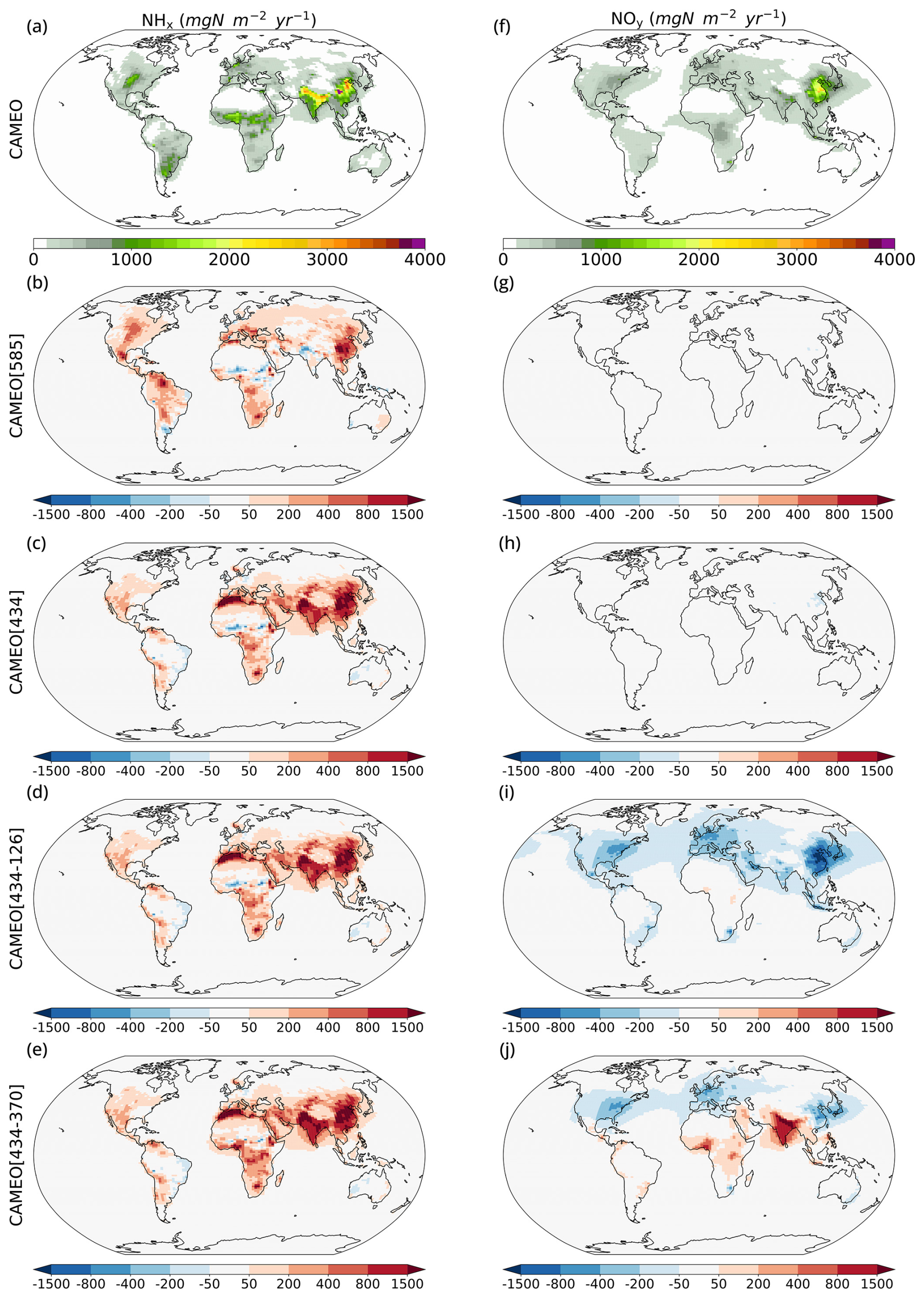
Figure 9 Mean annual surface depositions of NH_x and NO_y simulated in the CAMEO simulation (first row; over 2004–2014) and the anomalies between the CAMEO[SSPi] and CAMEO simulations ([SSPi] is for 585, 434, 434-126, and 434-370 in rows 2–5; over 2090–2100) ($\mathrm{mg}\mathrm{N}{\mathrm{m}}^{-\mathrm{2}}{\mathrm{yr}}^{-\mathrm{1}}$).

There are minimal spatial differences (<5 %) in the deposition of NO_y between CAMEO and CAMEO[434] (and CAMEO[585]), as constant NO_x emissions lead to a balancing effect, resulting in a decreased HNO₃ deposition and an increased ${\mathrm{NO}}_{\mathrm{3}}^{-}$ deposition, especially in China (see Fig. 9g and h). Under the low-NO_x scenario (CAMEO[434-126]), the NO_y deposition decreases all over the world, and the highest anomalies are located in China ($<-\mathrm{800}\mathrm{mg}\mathrm{N}{\mathrm{m}}^{-\mathrm{2}}{\mathrm{yr}}^{-\mathrm{1}}$). When future SSP3-7.0 emissions of NO_x are prescribed, the impact on NO_y deposition follows a similar pattern to the NO_x emissions. Compared to CAMEO, the deposition of NO_y in CAMEO [434-370] is significantly increased in India ($>\mathrm{800}\mathrm{mg}\mathrm{N}{\mathrm{m}}^{-\mathrm{2}}{\mathrm{yr}}^{-\mathrm{1}}$) and to a lesser extent in Africa and the Arabian Peninsula ($\sim \mathrm{300}\mathrm{mg}\mathrm{N}{\mathrm{m}}^{-\mathrm{2}}{\mathrm{yr}}^{-\mathrm{1}}$). Over the most developed countries, the NO_y deposition depicts negative anomalies of around 300 $\mathrm{mg}\mathrm{N}{\mathrm{m}}^{-\mathrm{2}}{\mathrm{yr}}^{-\mathrm{1}}$ (Fig. 9j).

5.3 Associated radiative forcing

The impact of the different future emissions on the total nitrate and sulfate AOD at 550 nm is presented in Fig. 10 and Table 6. The global increase in the nitrate AOD due to future NH₃ emissions from CAMEO ranges from 50 % to 100 % for CAMEO[434-370]. As mentioned in the previous section, considering the future SSP4-3.4 emissions from CAMEO, while keeping other emissions at their present-day levels (CAMEO[434]), positively impacts nitrate aerosol formation. This results in an increase in the total aerosol optical depth (AOD) ranging from 0.01 for most land and ocean areas to 0.05 over China. While sulfate AOD contributed the most to the total AOD with present-day-level emissions, the nitrate AOD becomes very important in CAMEO[434]. When considering strict regulations in the NO_x and SO₂ emissions as seen in CAMEO[434-126], the impact on the AOD is significant for the sulfate aerosol depth, where the decrease can reach −0.15 over China, for instance, compared to the CAMEO simulation. The positive impact on the nitrate AOD in this simulation is in the same range as the one in CAMEO[434], except in China, where the decrease in NO_x emissions leads to a decrease in the AOD of around 0.03. It is interesting to note that in CAMEO[434-126], the decrease in SO₂ emissions largely counterbalances the NO_x emission reductions as NH₃ is reacting with the sulfate in priority to form ammonium sulfate aerosols. Except in tropical Africa, where there is almost no impact of future emissions on the sulfate AOD, most of the land regions depict negative anomalies in the total AOD. Finally, the impact of future NO_x and SO₂ emissions from SSP3-7.0 combined with NH₃ emissions from SSP4-3.4 leads to a strong increase in the total AOD over Africa and India (around 0.10 and 0.15, respectively) and a slight decrease over the western US and Europe (around 0.03). The highest increases in the total AOD are explained by large positive anomalies in the nitrate and sulfate AOD (the impact on nitrate is around 3 times higher than on sulfate), while the negative patterns are mostly the result of negative anomalies in the sulfate AOD and slight changes in nitrate AOD. The different impacts on the total AOD inform us about the importance of not only considering ammonia behavior alone but also accounting for NO_x and SO₂, especially in the context of emission mitigation policies. It is important to note that global present-day nitrate AOD in CAMEO is twice as high (0.016; Table 6) as the six-model average quantified in the intercomparison from AeroCom phase III but close to the GISS one-moment aerosol (OMA) model estimate (0.015; Bian et al., 2017). However, global sulfate AOD in CAMEO (0.042) is in the recent model range (0.047) presented by Bian et al. (2017).

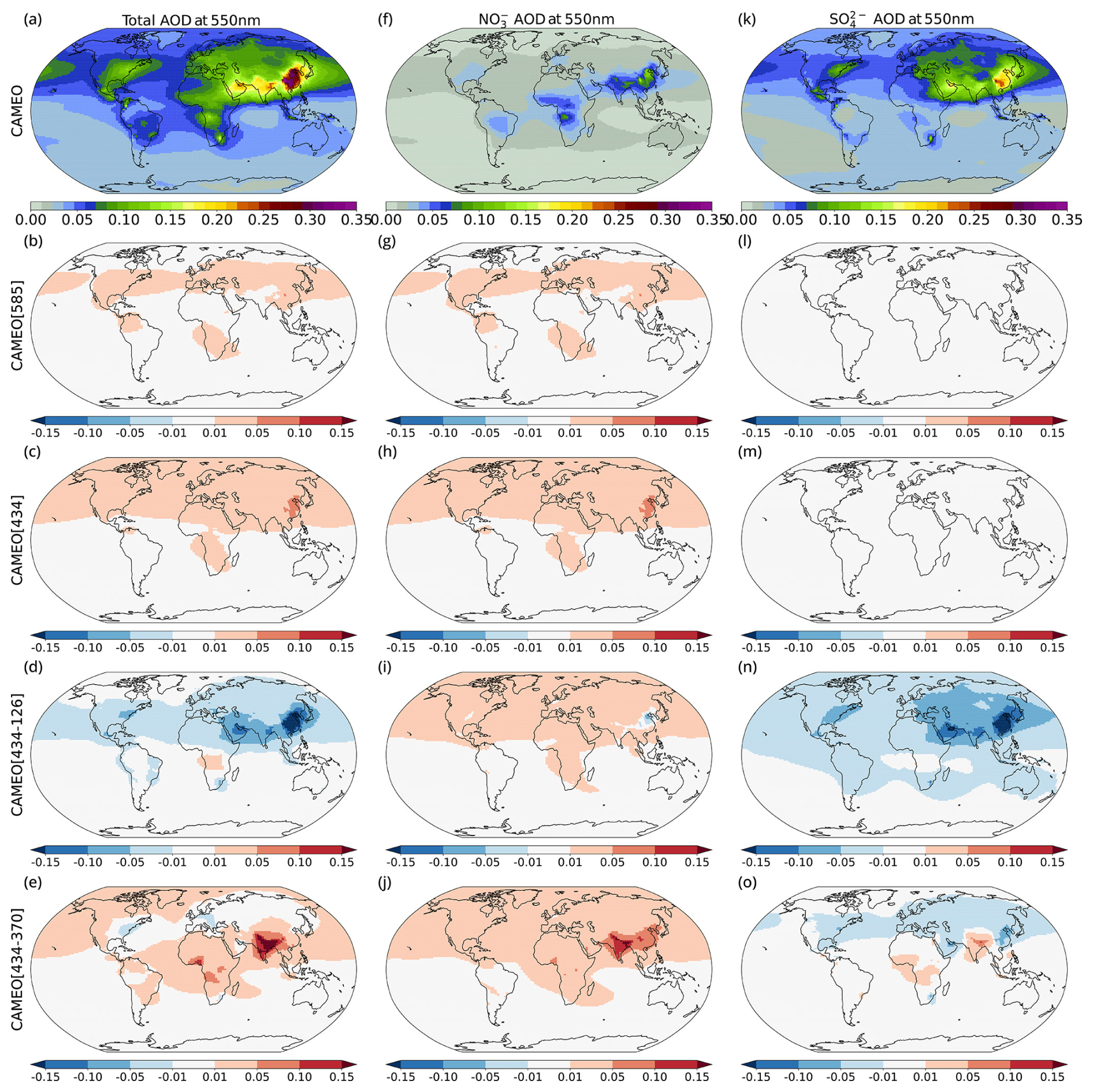
Figure 10 Mean annual total anthropogenic aerosol (i.e., nitrate + sulfate AOD; first column), nitrate aerosol (second column), and sulfate aerosol (third column) optical depths at 550 nm simulated in the CAMEO simulation (first row; over 2004–2014) and the anomalies between the CAMEO[SSPi] and CAMEO simulations ([SSPi] is 585, 434, 434-126, and 434-370 in rows 2–5; over 2090–2100).

Table 6 All-sky direct radiative forcing at the top of the atmosphere (RF TOA; mW m⁻²) and the aerosol optical depth (AOD) of the nitrate and sulfate aerosols since the present-day and future evolution under the different scenarios considered in this study. Note that for AOD, future evolution is given as ΔAOD, which is the difference between the future and present-day AODs.

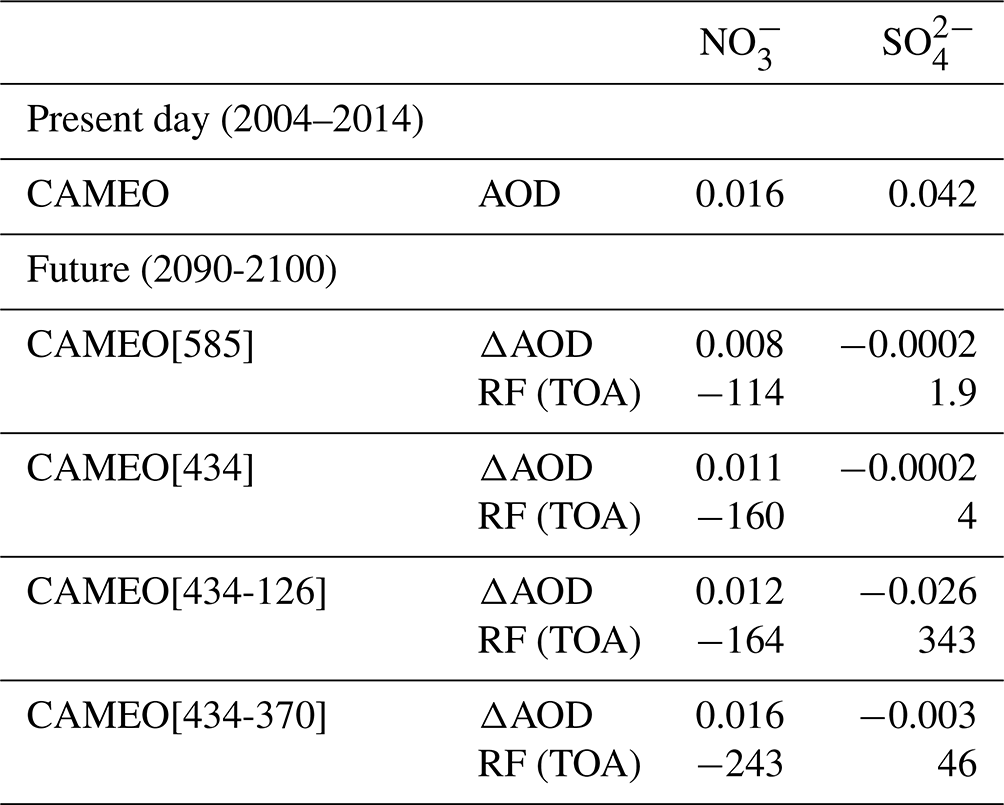
The all-sky direct radiative forcings at the top of the atmosphere (RF TOA) are presented in Table 6 and are calculated as the difference between the future considered CAMEO radiative fluxes and the historical CAMEO fluxes. Only replacing historical NH₃ emissions with those from SSP5-8.5 and SSP4-3.4 results in a net cooling of −114 and −160 mW m⁻² that is induced by nitrate aerosol radiative forcing and a slight positive warming from the sulfate forcing ($\simeq \mathrm{3}\mathrm{mW}{\mathrm{m}}^{-\mathrm{2}}$). The nitrate aerosol effects of the other experiments (CAMEO[434-126] and CAMEO[434-370]) are much more important (−164 and −243 mW m⁻²) than the highest anthropogenic radiative forcing calculated by Hauglustaine et al. (2014), which compares the scenario in RCP8.5 for 2100 with pre-industrial conditions (−115 mW m⁻²). The sulfate aerosol radiative effect is 7 times more important in CAMEO[434-126] (343 mW m⁻²) than in CAMEO[434-370], where NO_x and SO₂ emissions from SSP1-2.6 are highly slowed down in 2100.

5.4 Impact on N₂O production

The oxidation of ammonia with the hydroxyl (OH) radical into N₂O is an additional atmospheric pathway that can represent an important climate factor in the future. Multiple studies investigated the importance of the production of N₂O from NH₃, which can range from 0.60 to 1.8 Tg N₂O yr⁻¹ (Dentener and Crutzen, 1994; Kohlmann and Poppe, 1999; Hauglustaine et al., 2014; Pai et al., 2021). Our present-day production matches well with this range (1.6 Tg N₂O yr⁻¹, Table 5) and represents 15 % of the present-day total anthropogenic N₂O emissions used for CMIP6 (Gidden et al., 2018). However, considering that the natural soil emission contribution (10 Tg N₂O yr⁻¹) is as important as the total anthropogenic source, as estimated by Tian et al. (2024), our present-day production would in fact represent 8 % of the total N₂O emissions. When considering our highest future NO_x scenario (SSP3-7.0) combined with NH₃ emissions from SSP4-3.4, N₂O production accounts for 18 % (3.7 Tg N₂O yr⁻¹) of the future N₂O anthropogenic emissions (under SSP3-7.0; Gidden et al., 2018). This result is close to the 21 % quantified by Pai et al. (2021) using RCP trajectories for 2100.

6 Summary and conclusions

Because NH₃ impacts the nitrate aerosol and nitrous oxide levels in the atmosphere, changes in agricultural NH₃ emissions have important implications for climate and air quality. Regulating the agricultural sector is a challenge due to its importance in feeding the population, and thus, understanding the impact of future agricultural NH₃ emissions on the atmospheric chemistry is of high interest to design accurate mitigation emission scenarios. In this paper, the LMDZ–INCA global model is exploited to evaluate the impact of a new agricultural NH₃ emission dataset recently developed based on the ORCHIDEE LSM. This new dataset investigates the role played by NH₃ emissions in the atmosphere considering the dynamical environmental conditions and accounting for natural soil sources. The model results have been compared not only to NH₃ columns observed by the IASI instrument but also to surface concentrations measured by various observational networks. In addition, in LMDZ–INCA, tropospheric aerosols are also included through a representation of the sulfate nitrate–ammonium cycle and heterogeneous reactions between gas phase chemistry and aerosols. With this model, we investigate the impact of present-day and future (2090–2100) NH₃ emissions on atmospheric composition, N deposition fluxes, and climate forcing.

The key results of this paper are summarized as follows:

1. NH₃ emissions provided by CAMEO show good accuracy in the simulated NH₃ columns when evaluated against the IASI observations. Large reductions in the spatial model biases are noticeable compared to the reference version in which the CEDS inventory is prescribed. More specifically, the biases decreased by at least 50 % in Africa, Latin America, and the US. CAMEO emissions not only improved the spatial representation of the columns but also their seasonal cycle, especially in India, equatorial Africa, China, and South America, where the skill functions calculated for the temporal variability gained between 1 and 3 points compared to the CEDS simulation. Comparisons of the simulated surface observations with ground-based observations indicate that using CAMEO emissions improved the representation of annual NH₃ and ${\mathrm{NO}}_{\mathrm{3}}^{-}$ concentrations at the surface in 2015 in China, the US, and Canada. In Europe, the reduction in the NH₃ bias, however, does not lead to improvement in the aerosol representation compared to CEDS.

2. The impact of CAMEO NH₃ emissions on NH_x and NO_y deposition fluxes has been investigated. The global budget of NH_x is around 65 Tg N yr⁻¹, which is 20 % higher than the average calculated from other model-based estimates (CCMI, EMEP, MSC–W, and CEDS). The difference is mainly explained by enhanced deposition in Africa, which is twice as high as the deposition budget of the three alternative estimates. Due to relatively low nitrate levels and much higher NH₃ emissions in equatorial Africa, more NH₃ is removed through deposition processes, especially during the precipitation season when wet scavenging occurs more frequently. Despite differences with the EMEP and CCMI modeling results, a seasonal comparison at a specific measurement station from INDAAF in western Africa shows good agreement in the ${\mathrm{NH}}_{\mathrm{4}}^{+}$ wet deposition when CAMEO emissions are used in the LMDZ–INCA model.

3. Our analysis of the NH_x deposition seasonal cycle highlights some discrepancies in the simulated fluxes from CCMI, where seasonal variation is absent. The CCMI deposition dataset is a crucial forcing file for ESM, more specifically for land surface models. Even though the agricultural sector is the major driver for the NH₃ emission seasonality, the NH_x deposition can also play a role in more remote regions characterized by intensive precipitation seasons. The bi-directional flux of NH₃ can significantly impact NH₃ deposition, emission, re-emission, and atmospheric lifetime (Sutton et al., 2007). The interactive calculation of the different fluxes between the surface and the atmosphere has already been implemented in modeling approaches and shows significant improvements in the [NH₃], $\left[{\mathrm{NH}}_{\mathrm{4}}^{+}\right]$, $\left[{\mathrm{NO}}_{\mathrm{3}}^{-}\right]$, and ${\mathrm{NH}}_{\mathrm{4}}^{+}$ wet depositions at a regional and global scale (Pleim et al., 2019; Vira et al., 2020, 2022). This aspect motivates the implementation of a coupling based on a compensation point for NH₃ between LMDZ–INCA and ORCHIDEE, which is already under development. The ongoing coupling seems promising to address the overestimation from CAMEO emissions and the resulting NH₃ columns over the US and Europe in July.

4. Even though we are aware of some uncertainties and potential room for improvement, the model evaluation provides some confidence for using CAMEO emissions to investigate the impact of future NH₃ emissions on atmospheric chemistry and climate. We have constructed four future scenarios for 2090–2100 in which the impact of CAMEO emissions for SSP5-8.5 and SSP4-3.4 under different NO_x and SO₂ emission conditions has been studied. It is worth noting that as far as we know, no future gridded livestock and interactive soil emissions have been used to investigate future NH₃ emission perturbations on the atmospheric chemistry at the global scale.

5. Future CAMEO emissions lead to an overall increase in the global NH₃ burden ranging from 59 % to 235 %, while the ${\mathrm{NO}}_{\mathrm{3}}^{-}$ burden increases by 57 %–114 %, depending on the scenario. By analyzing the behavior of CAMEO[434] and CAMEO[585], we investigated the isolated impact of future divergent NH₃ emissions. Our results highlight small changes in the nitrate formation mainly over eastern Asia, more specifically China (+ 2 µg m⁻³), where nitric acid concentrations are high (${\mathrm{HNO}}_{\mathrm{3}}>\mathrm{6}\mathrm{\mu }\mathrm{g}{\mathrm{m}}^{-\mathrm{3}}$) and thus ammonium neutralization is possible. It leads to an increase of around 0.05 in the total nitrate and sulfate AOD in China and a global increase of 19 %. In CAMEO[434-126], in which NO_x and SO₂ emissions are highly decreasing compared to the present day, we observed important decreases in surface nitrate and sulfate aerosol concentrations, especially over China (−4 µg m⁻³). In this scenario, even though NH₃ emissions increase the global nitrate AOD (+0.016), the negative impact of sulfate aerosol AOD is more important (−0.026), which results in a total AOD reduction of 23 %. In CAMEO[434-126], the increase in the total nitrate burden and AOD indicates that despite less nitrate being formed at the surface, more nitrate is vertically uplifted in the upper troposphere. When combined with increased NO_x and SO₂ emissions, higher NH₃ emissions lead to an enhanced formation of aerosol ($+\mathrm{5}\mathrm{\mu }\mathrm{g}{\mathrm{m}}^{-\mathrm{3}}$ of ${\mathrm{NO}}_{\mathrm{3}}^{-}$) at the surface compared to present-day levels, as is the case over India in CAMEO[434-370]. Despite the decrease in NO_x and SO₂ emissions over China, the US, Europe, and Saudi Arabia, the total nitrate and ammonium burden is doubled due to the contribution from India as it is one of the largest hotspots in terms of aerosol ammonium nitrate precursors in this scenario. In addition, India and Africa are the regions experiencing the highest change in the total nitrate and sulfate AOD (+80 % to +100 %) due to a higher contribution of the nitrate AOD.

6. In addition to the impact on the air quality and climate, future NH₃ emissions have a positive impact on the total NH_x deposition fluxes over land and oceans (+35 %). As already mentioned, the coupling between LMDZ–INCA and ORCHIDEE would improve the representation of the N exchanges. In addition to the direct impact of climate change on the emissions and deposition fluxes, one could also expect a change coming from the land-use shift due to its influence on the deposition velocity for instance.

7. Radiative forcings associated with the aerosol formation in the different scenarios have been presented. The impact of future CAMEO emissions alone results in a net cooling from nitrate aerosols which ranges from −114 to −160 mW m⁻². By varying the future sulfate and nitrate emissions, the nitrate radiative effect can either overshoot (net total impact of −200 mW m⁻²) or be offset by the sulfate effect (net total impact of $+\mathrm{180}\mathrm{mW}{\mathrm{m}}^{-\mathrm{2}}$). As a comparison, Hauglustaine et al. (2014) estimated a negative radiative forcing from nitrate under RCP8.5 of around −115 mW m⁻² (as pre-industrial emissions state as the baseline). These results from CAMEO[434-126] and CAMEO[434-370] suggest a significant impact of the future evolution of the NH₃ emissions on the climate, depending on the mitigation measures that would be undertaken for NO_x and SO₂ emissions.

8. In addition to the aerosol radiative effect, N₂O production from the oxidation of NH₃ has been estimated to be non-negligible in the present day (1.6 Tg N₂O yr⁻¹) and could represent up to 18 % (3.7 Tg N₂O yr⁻¹) of the future N₂O anthropogenic emissions under our highest future NO_x scenario (SSP3-7.0). Even though agricultural production is one of the most significant sectors to impact the N cycle, the potential use of ammonia for low-carbon energy production is gaining attention. The emerging ammonia economy linked to hydrogen fuel has been estimated to produce an additional N₂O atmospheric source of 1 Tg N₂O yr⁻¹ when considering a high estimate of reactive N emissions from ammonia use in the energy sector (Bertagni et al., 2023). Knowing that there is 1 % atmospheric conversion of nitrogen in ammonia into N₂O, which was used in the latter study, and that our estimate ranges between 1.5 % and 2.25 %, depending on the scenario, we can expect a greater impact from the new global-scale ammonia economy.

7 Future directions: towards N interactions in ESM

In this study, the simulations are designed to isolate the impact of emission changes by keeping meteorological conditions fixed at present-day levels during 2090–2100. Climate change is expected to influence atmospheric chemistry through multiple interrelated factors, such as altered mean and extreme precipitation patterns that affect deposition, warming that could shift key chemical reactions, and wind variations that can affect aerosol transport. In a subsequent study, additional simulations will explore the combined impact of emissions and climate change by incorporating changing meteorological conditions for atmospheric chemistry.

Incorporating the nitrogen cycle into Earth system models is a recent advancement, as highlighted by Davies-Barnard et al. (2022). Developing interactions of nitrogen compounds is complex due to the intricate processes involved, necessitating readiness in coupling atmospheric chemistry and land components. The studies by Pleim et al. (2019) and Vira et al. (2020, 2022) provide a foundational step towards bi-directional ammonia handling, though this is not yet fully integrated into existing ESMs. Vira et al. (2022) notes that FANv2 does not currently feed back nitrogen losses to the nitrogen cycle in the Community Land Model, leaving fertilizer nitrogen availability to crops unaffected. Our present approach does include feedback from nitrogen loss affecting available soil nitrogen for vegetation, even without a bi-directional scheme yet being exploited. Additionally, in the CAMEO framework, we incorporated nitrogen biomass removal for livestock needs, ensuring nitrogen and carbon budget accuracy. Current efforts are focusing on developing nitrogen species exchanges at the atmosphere–surface interface in the IPSL ESM, aiming to assess chemical and climate impacts through interactive coupling.