Modeling actinic flux and photolysis frequencies in dense biomass burning plumes

Biomass burning (BB) affects air quality and climate by releasing large quantities of gaseous and particulate pollutants into the atmosphere. Photochemical processing during daylight transforms these emissions, influencing their overall environmental impact. Accurately quantifying the photochemical drivers, namely actinic flux and photolysis frequencies, is crucial to constraining this chemistry. However, the complex radiative transfer within BB plumes presents a significant challenge for both direct observations and numerical models.

This study introduces an expanded version of the 1D VLIDORT-QS radiative transfer (RT) model, named VLIDORT for photochemistry (VPC). VPC is designed for photochemical and remote sensing applications, particularly in BB plumes and other complex scenarios. To validate VPC and investigate photochemical conditions within BB plumes, the model was used to simulate spatial distributions of actinic fluxes and photolysis frequencies for the Shady wildfire (Idaho, US, 2019) based on plume composition data from the NOAA/NASA FIREX-AQ (Fire Influence on Regional to Global Environments and Air Quality) campaign.

Comparison between modeling results and observations by the CAFS (charged-coupled device actinic flux spectroradiometer) yields a modeling accuracy of 10 %–20 %. Systematic biases between the model and observations are within 2 %, indicating that the uncertainties are most likely due to variability in the input data caused by the inhomogeneity of the plume as well as 3D RT effects not captured in the model. Random uncertainties are largest in the ultraviolet (UV) spectral range, where they are dominated by uncertainties in the plume particle size distribution and brown carbon (BrC) absorptive properties.

The modeled actinic fluxes show a decrease from the plume top to the bottom of the plume with a strong spectral dependence caused by BrC absorption, which darkens the plume towards shorter wavelengths. In the visible (Vis) spectral range, actinic fluxes above the plume are enhanced by up to 60 %. In contrast, in the UV, actinic fluxes above the plume are not affected or even reduced by up to 10 %. Strong reductions exceeding an order of magnitude in and below the plume occur for both spectral ranges but are more pronounced in the UV.

1 Introduction

Biomass burning (BB) constitutes a major source of particulate and gaseous atmospheric pollutants with a significant impact on air quality and climate (Crutzen and Andreae, 1990; Bond et al., 2013; Klimont et al., 2017). As a consequence of climate change, natural BB events are expected to increase in frequency and intensity, thereby gaining even further significance in the coming decades (Jaffe et al., 2020; McClure and Jaffe, 2018; O'Dell et al., 2019). Particles emitted from BB primarily consist of black carbon (BC) and organic carbon (OC) (Reid et al., 2005; Levin et al., 2010), while emitted gases include carbon monoxide, nitrogen oxides, a plethora of volatile organic compounds, and greenhouse gases such as CO₂, CH₄, and N₂O (Andreae, 2019). During daytime, both BB particles and gases undergo photochemical processing in the plume, leading to the removal and transformation of emitted gases, formation of secondary pollutants, and changes in particle properties (Hand et al., 2010; Forrister et al., 2015; Sumlin et al., 2017; Peng et al., 2021; Xu et al., 2021; Liu et al., 2021; Hennigan et al., 2012; Cappa et al., 2020; Kiland et al., 2023). The main driver for these processes is photochemistry inside the plume, which is often optically thick and highly inhomogeneous. Consequently, the accurate quantification of the photochemical drivers is crucial to assessing the impact of biomass burning emissions on the environment.

Understanding and predicting the photochemistry in a given environment require knowledge of the speed at which the involved reactions proceed. For a photochemical reaction,

$$\begin{array}{}\text{(1)}& A+h\mathit{\nu }\to B+C,\end{array}$$

initiated by a photon hν, the reaction rate,

$$\begin{array}{}\text{(2)}& {\displaystyle \frac{\mathrm{d}\left[A\right]}{\mathrm{d}t}}=-J\left[A\right],\end{array}$$

is determined by the photolysis frequency J (expressed in Hz), which can be calculated according to

$$\begin{array}{}\text{(3)}& J=\int \mathit{\sigma }\left(\mathit{\lambda }\right)\mathrm{\Phi }\left(\mathit{\lambda }\right)F\left(\mathit{\lambda }\right)\mathrm{d}\mathit{\lambda }.\end{array}$$

The absorption cross-section σ(λ) of A describes the probability of photons being absorbed, while the quantum yield Φ(λ) is the probability of absorbed photons undergoing the reaction. σ(λ) and Φ(λ) are typically known from laboratory measurements. The actinic flux F(λ) describes the spherically integrated, directionally independent number of photons at wavelength λ. F(λ) is controlled by environmental factors, such as altitude, solar position, cloudiness, aerosols, and Earth surface properties. All of these conditions are temporally and spatially variable. Consequently, F(λ) is highly variable and its determination can be challenging.

Direct measurements of F(λ) can be performed with high accuracy using instruments with direction-insensitive reception optics and spectrometers that cover the required spectral and dynamic range (e.g., Junkermann et al., 1989; Kraus and Hofzumahaus, 1998; Shetter and Müller, 1999; Bais et al., 2003). However, such in situ measurements are limited in spatiotemporal coverage and are not performed on all aircraft missions studying trace gases or aerosols. Another, often complementary, approach is to simulate actinic fluxes using radiative transport (RT) models. With such models, continuous spatial distributions of actinic fluxes can be derived. RT models need to be constrained with detailed information on the atmospheric conditions, in particular on the spatial distribution and properties of clouds and aerosols. In chemical transport models the inputs for the built-in RT models are driven by the chemical transport simulation itself. For the interpretation of field experiments and observations, the compilation of adequate RT model input data is more challenging.

Over the past 50 years, both direct measurements of actinic fluxes and RT simulations have been applied to obtain a complete picture of the radiative conditions for clear-sky conditions (e.g., Turco, 1975; Meier et al., 1997; Shetter et al., 2002; Volz-Thomas et al., 1996; Hofzumahaus et al., 2002; Wagner et al., 2011) and above, below, and inside clouds (e.g., Thompson, 1984; Madronich, 1987; Junkermann, 1994; Kelley et al., 1995; Lefer et al., 2003; Tie et al., 2003; Liu et al., 2006; Neu et al., 2007; Ryu et al., 2017). In contrast, for BB plumes, corresponding studies rely on observations only, whereas the modeling of actinic fluxes and photolysis frequencies and their spatial distribution has received less attention. For instance, many current experimental BB plume chemistry studies are based on directly measured actinic fluxes (Decker et al., 2021; Liao et al., 2021) or irradiances (e.g., Lindsay et al., 2022) or on the deduction of actinic fluxes from concentration measurements of gases involved in well-known proxy reactions (Peng et al., 2021). Such measurements are, however, limited in spatiotemporal coverage as they can only provide information at a single location and time. For atmospheric chemistry studies in BB plumes, a more complete picture is desirable, as the high spatial variability of actinic fluxes and photolysis frequencies significantly impacts plume processing (e.g., Decker et al., 2021; Palm et al., 2021). Continuous distributions of actinic flux and photolysis frequencies with the required accuracy and spatial resolution can only be inferred using RT models. Trentmann et al. (2003) and Trentmann (2003) performed such RT modeling, but only for a synthetic BB plume created with a 3D chemical transport model. To our knowledge, similar studies for real plume scenarios do not currently exist. This is not surprising, as modeling is typically challenged by a lack of information to constrain the RT model, arising from the complex and variable nature of such plumes, in particular when they are young (hours old) and optically dense. The RT in BB plumes is dominated by aerosol, for which the spatial distributions and optical properties are often not well-known. A peculiarity in BB plumes is the optically active fraction of OC, typically referred to as “brown carbon” (BrC), which becomes strongly absorbing towards shorter wavelengths (Laskin et al., 2015). It dominates the RT in the ultraviolet (UV) spectral range, where photochemistry is most responsive. Its concentrations and optical properties are difficult to assess, as they depend on the burned fuel, burning phase, and smoke age (Forrister et al., 2015; Laskin et al., 2015; Sumlin et al., 2018; Zeng et al., 2022; Shetty et al., 2023).

In addition, challenges arise from the modeling side. In the presence of optically thick clouds or plumes, horizontal transport effects such as side illumination and shadowing can significantly impact the radiation field, particularly when spatial scales on the order of the cloud size or smaller have to be resolved (Stephens and Platt, 1987; Mayer, 2009; Wagner et al., 2023). Considering such effects requires 3D RT models (e.g., Mayer, 2009; Deutschmann et al., 2011), which are computationally expensive. Most models, including the model used in this study, therefore assume a horizontally homogeneous atmosphere; they solve the radiative transfer equation in one dimension and are thus referred to as “1D RT models”. This assumption strongly increases efficiency but can introduce errors due to the inability to simulate RT in the horizontal dimension. Investigations of these effects have been performed based on synthetic data (Trentmann, 2003), showing the significance of shadowing. 1D RT models, and to a certain extent 3D models, often suffer from incomplete knowledge and a simplified description of the input data, particularly in complex environments where atmospheric inhomogeneities can introduce uncertainties in the model initialization. These inhomogeneity effects and challenges with horizontal RT in real BB plume scenarios have not been well-studied. There is thus a need to better understand how well 1D RT models can describe actinic fluxes and photolysis frequencies in these plumes.

The accuracy of modeled actinic fluxes and photolysis frequencies can only be ensured by comparison with established models or with measurements. While such comparisons have been conducted extensively for well-defined atmospheric scenarios (e.g., Barnard et al., 2004; Kelley et al., 1995; Castro et al., 1997; Volz-Thomas et al., 1996; Dickerson et al., 1997; Kazantzidis et al., 2001; Vuilleumier et al., 2001; Balis et al., 2002; Shetter et al., 2003; Hofzumahaus et al., 2004), they have not been performed for the complex radiative conditions encountered in optically dense BB plumes.

In the present study we derive continuous spatial distributions of actinic flux and photolysis frequencies in a real and optically dense BB plume by means of RT simulations. The key objectives of the study are the following:

1. Introduce and validate a recently developed radiative transfer model (VPC) for photochemical and remote sensing applications in BB plumes.

2. Assess the viability and limitations of actinic flux and photolysis modeling in BB plumes using 1D RT models and state-of-the-art plume composition measurements.

3. Provide insights into spatial actinic flux and photolysis frequency distributions in BB plumes.

The VPC model (Sect. 2) is an extended version of the VLIDORT-QS model (Spurr, 2006), a variant of the widely used VLIDORT RT model. VPC can calculate actinic fluxes based on a range of input parameters. We constrain VPC using recent airborne BB plume composition measurements performed during the FIREX-AQ campaign in 2019 (Sect. 3) to simulate 2D distributions of actinic flux and photolysis frequencies over 20 plume cross-sections (Sect. 4). We compare these modeling results to FIREX-AQ actinic flux and photolysis frequency measurements to validate the VPC results (Sect. 5) and to quantify systematic and random uncertainties. We investigate spectral and environmental dependencies and perform model sensitivity studies to identify critical factors that limit the modeling accuracy. In addition, we investigate selected model results to provide deeper insight into the spatial and spectral distribution of actinic fluxes and photolysis frequencies in BB plumes (Sect. 6). Potential implications and future studies in BB plume radiative transport, chemical modeling, and remote sensing applications are discussed at the end of this paper (Sect. 6).

2 Model description

VLIDORT for photochemistry (VPC) is built around the Quasi-Spherical Vector Linearized Discrete Ordinate Radiative Transfer (VLIDORT-QS) code (Sect. 2.1). The VLIDORT family of RT codes is widely used in the trace gas remote sensing community (Spurr, 2006; Spurr and Christi, 2019). These codes have been tested for many different atmospheric conditions and are thus well-suited for the study and interpretation of field observations. While there are other well-established and efficient RT models for the calculation of photolysis frequencies, such as the Tropospheric UV and Visible (TUV) radiation model Fortran code (Madronich and Flocke, 1999) or Fast-J (Wild et al., 2000), VPC particularly facilitates the interpretation of field observations of BB plumes. To allow the study of dense BB plumes, VPC has to meet the following requirements: (1) a suitable and flexible representation of BB plume particles in the model, (2) efficient retrieval and sensitivity analyses common in remote sensing studies, (3) accurate RT results for a wide variety of geometries, including high solar zenith angles (SZAs) and limb viewing directions, (4) simulation of the light's polarization state, allowing for retrieval of aerosol information from polarimetric remote sensing data (which will be explored in future studies), and (5) the simultaneous calculation of radiances and actinic fluxes, useful for applications where actinic fluxes are deduced from radiance observations or where photochemistry and remote sensing are closely linked (e.g., for plume composition measurements from a satellite).

An overview of the model is depicted in Fig. 1. On the input side, VPC features the so-called “aerosol module”, designed to describe complex aerosol mixtures in a flexible way: the module allows usage of an arbitrary number of aerosol types, each with individual properties that are described either via bulk optical or microphysical parameters (see Sect. 2.2.2 for details). On the output side, a module has been added to convert the RT-simulated actinic flux spectra to photolysis frequencies for various chemical reactions (Sect. 2.4). VLIDORT-QS, the photolysis frequency module, and parts of the aerosol module are implemented in Fortran but have been embedded in object-oriented Python wrappers to obtain a structured and modular user interface, including useful functions for data pre- and post-processing as well as visualization. The package supports not only combined use but also stand-alone individual use of the aerosol, VLIDORT-QS, and photolysis frequency modules. The current model default configuration is optimized for tropospheric applications in the wavelength range between 295 and 650 nm. Extension to stratospheric applications requires adding additional absorbers (e.g., O₂ absorption in the deep UV).

Figure 1 Schematic of the VPC model.

2.1 VLIDORT-QS radiative transport model

The core of VPC is the VLIDORT-QS radiative transfer code, which is designed for a spherically curved atmosphere. Single scattering (or first-order radiative transfer) is treated exactly for a spherically curved medium, while multiple-scattering radiation fields along a given line of sight are calculated using a modified version of the standard VLIDORT model (Spurr, 2006) working in plane-parallel scattering mode. A detailed description of the VLIDORT-QS model, including validations against 3D Monte Carlo RT models, can be found in Spurr et al. (2022).

Since the original work on VLIDORT-QS was reported, we have added a number of additional features to the model. Most important for the present study is the ability to generate directionally integrated fluxes (actinic fluxes and irradiances) at all segment boundaries. The model also features a complete linearization scheme; i.e., in addition to the radiation field itself VLIDORT-QS will generate a complete range of analytically derived radiance or Stokes-vector Jacobians (weighting or sensitivity functions) with respect to any atmospheric parameter, including aerosol loading and optical properties in BB plumes. This capability makes VLIDORT-QS suitable for retrieval and sensitivity analyses common in remote sensing studies and adds this ability to observations of actinic fluxes. Finally, a number of performance enhancements have been made in order to speed up the calculations; in particular the code has been made thread-safe for use in parallel-computing environments such as OpenMP.

2.2 Model inputs

Table 1 provides an overview of the most relevant model input parameters, which are discussed in more detail in the following subsections.

Table 1 Overview of VPC input parameters. The index l indicates parameters defined individually for each atmospheric model layer. λ indicates a dependence on wavelength (see Sect. 2.5 for further details). Aerosol parameters are defined for each aerosol type $a=\mathit{\{}\mathrm{1},\mathrm{2},\mathrm{3},\mathrm{\dots }\mathit{\}}$. Parameters with an index $m=\mathit{\{}\mathrm{1},\mathrm{2},\mathrm{3}\mathit{\}}$ need to be specified for each mode of the trimodal PSD.

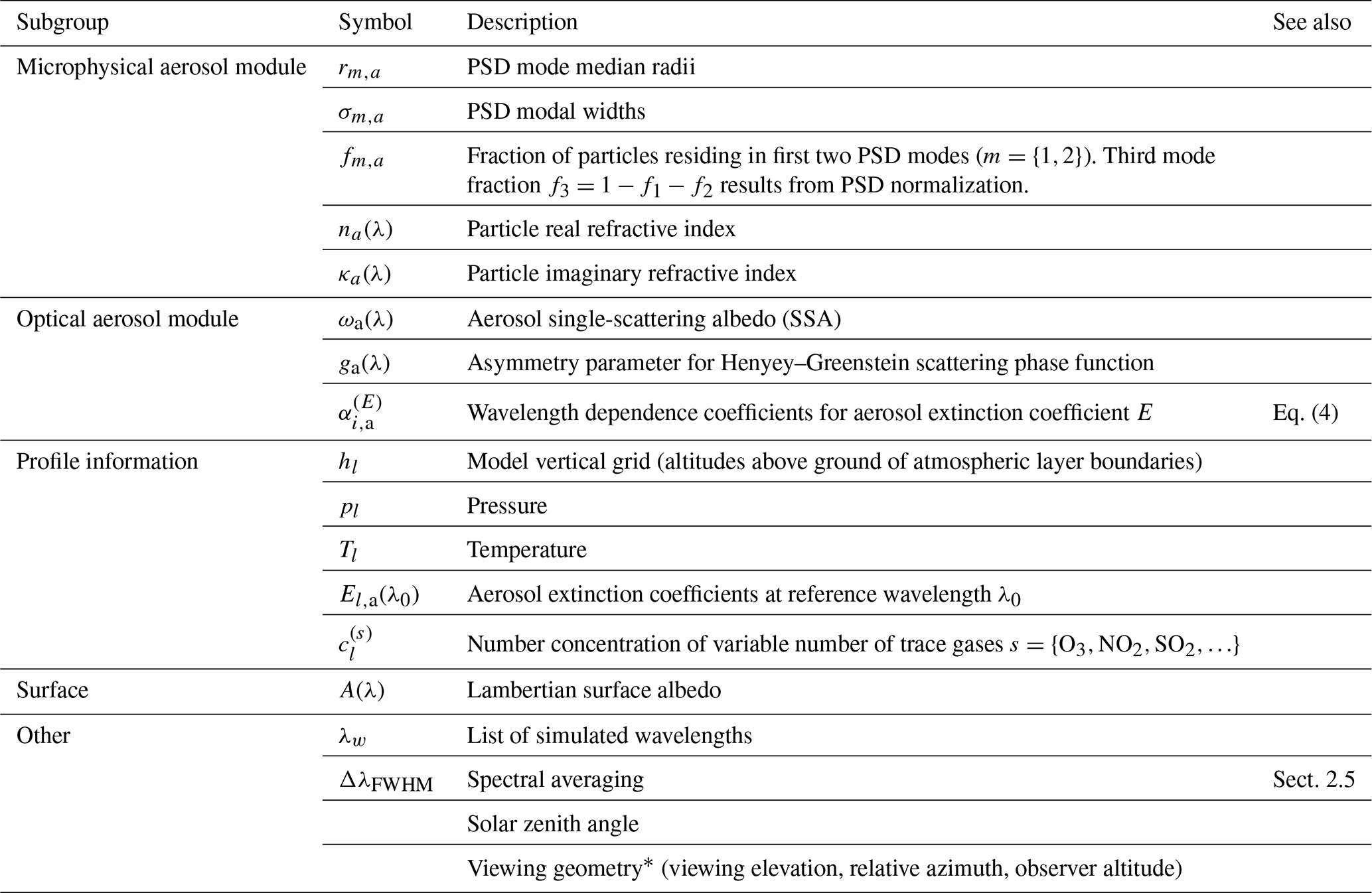
^* Of relevance for radiance calculations only.

2.2.1 Vertical grid

In VPC the atmosphere is represented by a finite number of stacked optically homogeneous layers. Common layer numbers are on the order of 100 over an altitude range from zero to about 70 km a.s.l. Layer thicknesses typically increase with altitude from about 100 m at the surface to several kilometers at the top of the atmosphere (e.g., Madronich and Flocke, 1999). By default, heights h_l for each layer boundary $l=\mathit{\{}\mathrm{0},\mathrm{1},\mathrm{\dots },l_{max}\mathit{\}}$ are defined via $h_l=c_{\mathrm{1}}(c_{\mathrm{2}}^l-\mathrm{1})$, resulting in an exponential grid with increasing layer thickness, but VPC also allows for user-defined arbitrary vertical grids.

2.2.2 Aerosol module

In the RT simulation performed with VLIDORT-QS, particles are described by a single set of effective bulk aerosol optical properties, namely the extinction coefficient, single-scattering albedo (SSA), and scattering phase matrix. The purpose of the aerosol module is to pre-calculate these quantities for mixtures of aerosol types with different properties. The module allows including an arbitrary number of aerosol types in the RT simulation. As described in detail in the following paragraphs, for each aerosol type the user chooses between two available aerosol models, provides aerosol properties as required by the respective model, and defines the aerosol vertical distribution.

The two available aerosol models are in the following referred to as the microphysical and optical aerosol model (Fig. 1). The microphysical aerosol model describes aerosol in terms of a particle size distribution (PSD) and complex particle refractive index (real part n and imaginary part κ). These are fed to an integrated Mie aerosol model (Spurr et al., 2012) to derive exact bulk optical properties, including the exact scattering phase matrices, assuming spherical particles. The PSD is trimodal, with up to three lognormal distributions. The (normalized) number of particles residing in each mode is described by the modal fractions f_m, with $f_{\mathrm{1}}+f_{\mathrm{2}}+f_{\mathrm{3}}=\mathrm{1}$. In the current VPC version, the Mie model assumes homogeneous particles, i.e., without coatings. Internally or externally mixed aerosols are realized by defining a single internally mixed aerosol type or multiple externally mixed aerosol types with individual properties, respectively. In the presented study we make use of the latter approach (Sect. 4). In the future, the microphysical model will be expanded to account for coated or non-spherical particles (see, e.g., Kattawar and Hood, 1976; Borghese et al., 1979; Mackowski and Mishchenko, 1996; Muinonen et al., 1996).

For some applications, e.g., remote sensing retrievals with limited information in the measurements, it is useful to stay in the optical domain and skip the additional layer of complexity added by a microphysical aerosol representation. This is the purpose of the optical aerosol model, wherein aerosol is described by the wavelength dependence coefficients ${\mathit{\alpha }}_{i,\mathrm{a}}^{\left(E\right)}$ (Eq. 4) and the SSA ω_a(λ). The scattering phase function is defined via the scattering asymmetry parameter (AP) g_a(λ), assuming a Henyey–Greenstein formalism (Henyey and Greenstein, 1941).

The properties of each aerosol type are constant with altitude. Altitude dependencies are realized via superposition of multiple aerosol types with different vertical profiles. To simplify the interpretation of field observations in VPC, aerosol amounts are expressed in terms of the aerosol extinction coefficient E_l,a(λ₀) (extinction per kilometer). Extinction coefficients are often provided by remote sensing observation. They are fed to the model for a specific reference wavelength λ₀ for each model layer l and each aerosol type a.

2.2.3 Trace gas absorption

For the radiative transport simulation, VPC includes literature cross-sections for O₃ (Brion et al., 1998), O₄ (Thalman and Volkamer, 2013), H₂O (Rothman et al., 2010; Lampel et al., 2015), and NO₂ (Vandaele et al., 1998). Users can provide vertical concentration profiles for each of these gases to account for their absorption. VPC also facilitates the implementation of additional gases.

2.2.4 Atmospheric boundaries

For the extraterrestrial solar irradiance at the top of the atmosphere (TOA), VPC users can choose to use either the spectrum by Chance and Kurucz (2010) or by Coddington et al. (2023). Surface properties in VLIDORT-QS can be defined via a Lambertian equivalent reflectance (LER) or by providing the full bidirectional reflectance distribution function (BRDF). In the current VPC framework only the wavelength-dependent LER is implemented. If required, BRDF functionality might be added in the future.

2.3 Wavelength-dependent parameters

Some model input parameters depend on wavelength, such as refractive indices, albedos, the extinction coefficient, and the asymmetry parameter. In this section we refer to them by x(λ). For each wavelength-dependent parameter, the model offers two approaches:

1. Providing independent values for a set of discrete wavelengths.

2. Providing a single value x₀ for a reference wavelength λ₀ and coefficients α_i for an Ångström wavelength dependence of arbitrary order i_max.

In the second case, parameter values for each wavelength are internally calculated assuming

$$\begin{array}{}\text{(4)}& \ln \left({\displaystyle \frac{x}{x_{\mathrm{0}}}}\right)=\sum _{i=\mathrm{1}}^{i_{max}}{\mathit{\alpha }}_i{\left(\ln {\displaystyle \frac{{\mathit{\lambda }}_{\mathrm{0}}}{\mathit{\lambda }}}\right)}^i.\end{array}$$

This parameterization represents an extended version of the classic Ångström wavelength dependence (Ångström, 1929). In fact, for i_max = 1, Eq. (4) can be rearranged to obtain the well-known dependence

$$\begin{array}{}\text{(5)}& {\displaystyle \frac{x}{x_{\mathrm{0}}}}={\left({\displaystyle \frac{\mathit{\lambda }}{{\mathit{\lambda }}_{\mathrm{0}}}}\right)}^{-{\mathit{\alpha }}_{\mathrm{1}}}.\end{array}$$

Increasing i_max to 2 adds a quadratic term to Eq. (4), effectively accounting for a log-linear wavelength dependence of the Ångström parameter, similar to parameterizations proposed by King and Byrne (1976), Kaufman (1993), and Schuster et al. (2006). Increasing i_max adds higher-order wavelength dependencies. The parameterization was chosen because of its general applicability. We found that Eq. (4) can successfully capture wavelength dependencies not only of extinction but also other parameters, such as SSA, AP, and aerosol refractive indexes measured during FIREX-AQ (see Sect. S1 in the Supplement). In contrast to the conventional Ångström dependence, Eq. (4) can also describe the strong non-log-linear wavelength dependence of BrC absorption in BB plumes.

As described in Sect. 2.2.2, aerosol vertical profiles are provided in terms of the extinction coefficient E(λ₀) at a reference wavelength λ₀. The wavelength dependence of E(λ) is either derived from internal Mie model calculations, when using the microphysical aerosol model, or according to Eq. (4), when using the optical aerosol model. In the case of the SSA ω, Eq. (4) was found to better describe (i.e., with lower i_max values) the single-scattering co-albedo 1−ω instead of ω itself. Thus, in the optical aerosol model Eq. (4) is applied to 1−ω.

2.4 Model outputs

The main outputs of an RT simulation with VLIDORT-QS are actinic flux spectra F_l(λ) at each layer boundary of the model's vertical grid. Separate spectra are provided for three contributions to F_l(λ):

1. Direct solar beam, attenuated by atmospheric extinction

2. Downwelling diffuse radiation, describing the quantity of scattered photons incident from the hemisphere above the observer

3. Upwelling diffuse radiation, describing the quantity of scattered photons incident from the hemisphere below the observer

This separation is useful as it allows for deeper analysis of the results, also considering that real measurements are typically performed separately for upwelling (diffuse only) and downwelling (direct + diffuse) actinic fluxes.

In addition, radiance spectra for a prescribed viewing geometry are calculated in the same simulation process (see Table 1). VLIDORT-QS and the Mie model feature an analytical linearization scheme (see, e.g., Spurr et al., 2022), which can provide Jacobians (sensitivities) of the outputs with respect to any input parameter with high computational efficiency.

For the conversion of actinic flux spectra to photolysis frequencies (performed by the “PF module”; see Fig. 1), we isolated and adapted a corresponding module from TUV (version 5.4) (Madronich and Flocke, 1999). It reads and prepares all required cross-sections and quantum yields to calculate photolysis frequencies for 113 photochemical reactions based on Eq. (3). Using this established code as a basis ensures consistency with the atmospheric chemistry community. We made a few adaptations: we added missing data on the N₂O₅ absorption cross-section for the 340 to 410 nm range, and we adapted ClNO₂ cross-section and quantum yield based on the 2015 JPL recommendations (Burkholder et al., 2019). Furthermore, we extended the module by including 14 additional reactions for halogen chemistry.

The TUV module was also used to process the measured actinic flux spectra from FIREX-AQ (see Sect. 3.3). Note that for the present study, only 48 photolysis reactions relevant to the spectral range of the measurements were considered. An overview of all of the reactions available is provided in Sect. S5.

2.5 Spectral averaging and interpolation

RT simulations can be performed for user-defined sets of wavelengths. Ideally, actinic flux spectra are calculated line by line, at a resolution resolving even narrow solar Fraunhofer and atmospheric absorption lines (on the order of a few picometers in the UV–Vis). However, using very small wavelength intervals is inefficient. On the other hand, subsampling the wavelength range decreases the accuracy of the simulation (e.g., Madronich and Weller, 1990). A number of steps have therefore been taken to make VPC flexible and more efficient. The resolution of the originally highly resolved (Δλ ≈ 0.01 nm) literature spectra used by the model (Sect. 2.2.3 and 2.2.4) can be reduced prior to simulation by Gaussian smoothing, i.e., convolution of the spectra with a Gaussian kernel of defined width, typically on the order of 1 nm FWHM (full width at half maximum). This option is useful for efficient calculation of outputs averaged over wavelength intervals of a few nanometers (nm), at the cost of relatively small errors, introduced by the commutation of RT modeling and spectral smoothing. We found < 1 % (< 3 %) errors in the photolysis frequencies for a smoothing kernel of 1 nm (2 nm) FWHM and typical atmospheric scenarios.

To improve efficiency further, a novel spectral interpolation approach was developed; this allows reproduction of high-resolution (Δλ ≈ 1 nm) actinic flux spectra from simulations at a few suitable wavelengths. Several models use approaches for efficient photolysis rate calculation by reducing the number of full radiative transport calculations to a few wavelengths (< 10) (e.g., Landgraf and Crutzen, 1998; Williams et al., 2006; Wild et al., 2000; Madronich and Flocke, 1999). They are, however, limited in accuracy (≈ 10 % in photolysis frequencies in the UV) and optimized for applications in clean atmospheres. Our approach uses more wavelengths (10 to 30, depending on SZA and atmospheric conditions) and is thus slower but more accurate (< 2 % error in photolysis frequencies), and it provides high-resolution spectra as an intermediate product. Furthermore, it also works for the particular conditions encountered in this study, including the presence of the strongly wavelength-dependent BrC absorption and high SZAs.

Our approach is inspired by the passive differential optical absorption spectroscopy (DOAS) measurement technique (Platt and Stutz, 2008). The passive DOAS approach measures radiances of scattered skylight, but the basic concepts described in the following hold for both radiances and actinic fluxes. Most of the structures observed in an actinic flux spectrum F(λ) are solar Fraunhofer lines already present in the extraterrestrial solar irradiance spectrum I₀. The actual atmospheric signal can be isolated and conveniently described by the actinic flux optical depth (AFOD):

$$\begin{array}{}\text{(6)}& \mathit{\tau }\left(\mathit{\lambda }\right)=-\ln \left({\displaystyle \frac{F\left(\mathit{\lambda }\right)}{I_{\mathrm{0}}\left(\mathit{\lambda }\right)}}\right).\end{array}$$

We make use of the fact that only trace gas absorption introduces significant narrowband features in τ(λ), whereas scattering and aerosol absorption impose a spectrally smooth signal. Therefore, just as for passive DOAS radiance OD spectra, AFOD spectra can be approximated by

$$\begin{array}{}\text{(7)}& \mathit{\tau }\left(\mathit{\lambda }\right)=\sum _{i=\mathrm{0}}^{n_p}{P}_i{\mathit{\lambda }}^i+\sum _s{S}_s\left(\mathit{\lambda }\right)\cdot {\mathit{\sigma }}_s(\mathit{\lambda },T_s).\end{array}$$

Here, the first term represents a polynomial that accounts for the spectrally smooth scattering and aerosol absorption signals. The second term accounts for optical depth contributions of each trace gas species s with absorptions strong enough to significantly influence actinic fluxes. σ^(s)(λ,T_s) represents the trace gas absorption cross-sections from the literature, which can depend on the gas temperature T_s. S^(s)(λ) is the observed slant column density (SCD), which is the gas concentration integrated along the effective light path. The term “effective” is used here to indicate that contributing photons travel along an infinite number of light paths, each with a distinct probability. These probabilities change with wavelength, as do the effective light path lengths and the SCD. Following Puķīte et al. (2010), we parameterize the SCD wavelength dependence by

$$\begin{array}{}\text{(8)}& S\left(\mathit{\lambda }\right)=\sum _{j=\mathrm{0}}^{n_{\mathit{\lambda }}}{S}_{\mathit{\lambda },j}{\mathit{\lambda }}^j+\sum _{k=\mathrm{1}}^{n_{\mathit{\sigma }}}{S}_{\mathit{\sigma },k}\mathit{\sigma }\left(\mathit{\lambda }\right),\end{array}$$

where we omitted the index s for readability. The first sum is a polynomial, with coefficients S_λ. It describes the SCD including a spectrally smooth wavelength dependence that arises from changes in RT due to scattering and aerosol absorption. S_σ accounts for changes in effective light path due to strong narrowband gas absorption, which favors short light path lengths through the absorbing gas.

In our case O₃ is the only absorbing gas of relevance. Then, Eqs. (7) and (8) describe any actinic flux spectrum based on $n_p+n_{\mathit{\lambda }}+n_{\mathit{\sigma }}+\mathrm{1}$ free parameters, including T_s. These parameters can be inferred by fitting Eq. (7) to simulated AFODs at a few suitable wavelengths. From the retrieved parameter values, the full high-resolution spectrum can be reconstructed.

The optimization of the interpolation settings applied for this study, as well as an accuracy assessment, is described in detail in Sect. S2. In short, we use simulations at 23 wavelengths to reproduce high-resolution actinic flux spectra (Δλ = 2 nm from 298 to 640 nm). Typical differences from the exact line-by-line calculated spectra were assessed for a wide range of conditions, yielding a root mean square deviation (RMSD) of 0.3 %. Maximum differences are observed in the UV and for SZAs > 80° but never exceed 7 %. Resulting errors in photolysis frequencies are even smaller, with a RMSD of 0.2 % and a maximum of 1.8 %. We therefore conclude that errors introduced by the interpolation are negligible compared to other sources of uncertainty encountered in the present study.

In the future, more investigations, similar to those in Sect. S2, can be performed to further enhance efficiency and make the interpolation generally applicable for other spectral ranges, spectral resolutions, and conditions.

3 Measurement data

The present study is based on data from the 2019 NOAA/NASA FIREX-AQ measurement campaign (Warneke et al., 2023). In the course of this 6-week airborne campaign, more than 90 BB plumes were sampled in situ as well as remotely from the NASA DC-8 research aircraft. For our purpose, the FIREX-AQ observations offer a unique opportunity, as they provide a view of plume composition and radiative conditions of unprecedented comprehensiveness and accuracy. An overview of all of the instruments aboard the aircraft and the raw data is available in the NASA FIREX-AQ data archive (Aknan and Chen, 2023). This section provides basic information on the flight selected for our analysis and instrumentation relevant for our study.

3.1 Shady fire overview

Our case study focuses on measurements from the “Shady fire” on 25 July 2019 in Idaho, which we chose for various reasons. Compared to other fires, the data coverage is high. The multiple-hour-long flight included three plume overflights as well as 20 plume transects during daylight and clear-sky conditions. Most instruments successfully collected data throughout the entire flight. The burned area over the sampling period was small (≈ 2 km²) and the burned fuel was homogeneous. The plume was large with an extent of about 10 km × 1 km × 100 km (W × H × L), ensuring good spatial sampling despite the high aircraft speed (≈ 150 m s⁻¹) and justifying the 1D model assumption of a horizontally homogeneous atmosphere. Observed solar azimuth angles (SAAs) were between 250 and 290°, and the sun is therefore almost aligned with the plume axis (270° azimuthal orientation) over the entire flight (Fig. 2), which is a favorable configuration for avoiding horizontal radiative transport effects (Sect. 6). Wind conditions were very stable. At the sampling altitude (4200 to 5200 m m.s.l.), transect-averaged wind speed and wind direction over the entire flight were 9 ± 3 m s⁻¹ and (270 ± 12)°. At the same time, a constantly low relative humidity of (32 ± 5) % prevented excessive hygroscopic growth of the aerosol particles. All in all, the Shady fire represents a particularly favorable case. Even though it might not represent typical conditions, it is an ideal starting point for our purposes, as model validation and error analysis occur in a comparably controlled environment. Future applications of the presented modeling approach to other plumes under less favorable conditions are discussed in Sect. 7.

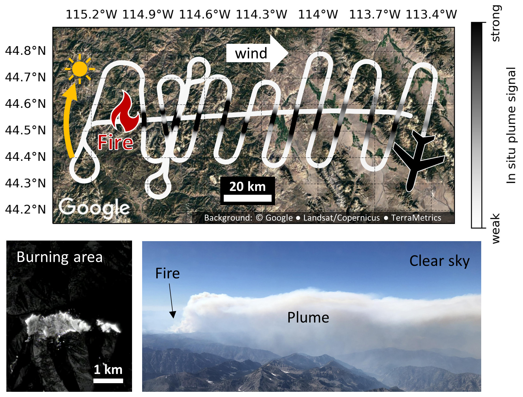
Figure 2 The upper panel shows the Shady fire geolocation and a part of the flight track (see the red box in Fig. 3), including an overflight along the plume axis and following transects. The approximate location and movement of the sun during the flight are indicated on the left. The lower left shows a nadir infrared image of the burning area (Aknan and Chen, 2023), recorded from the aircraft at the end of the second overflight.

Figures 2 and 3 provide a general overview of the conditions, fire location, and flight path. Plume overflights were performed against the wind along the plume axis and were followed by plume transects at progressively increasing distances from the fire.

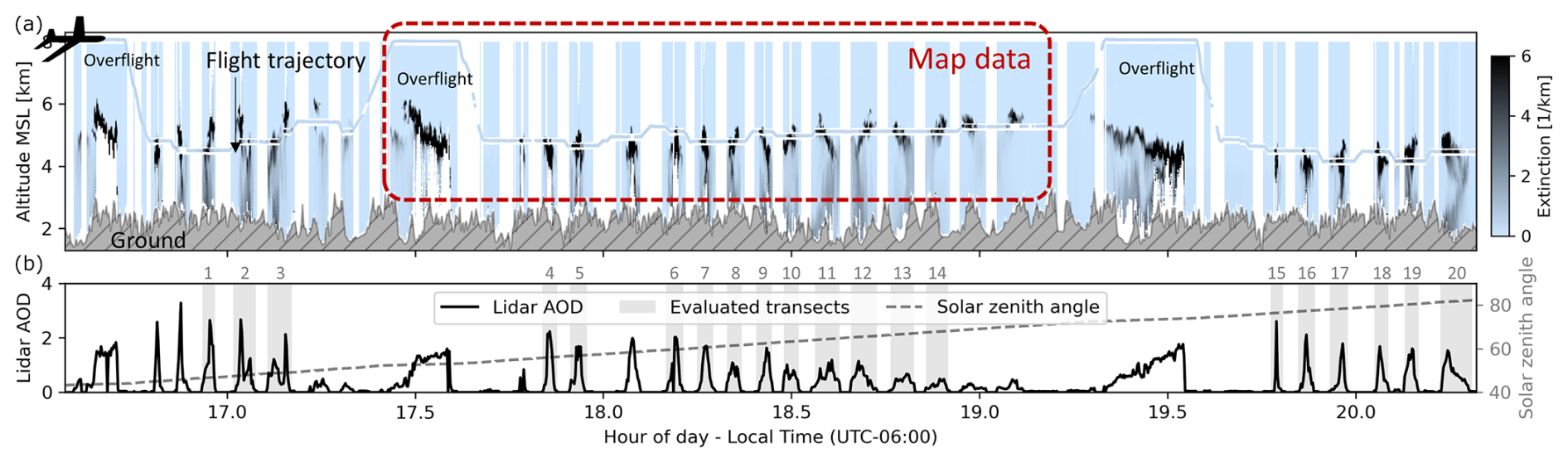
Figure 3 The Shady fire sampling flight profile. Panel (a) shows aerosol extinction profiles from the lidar. The flight track is embedded and color-coded based on in situ aerosol extinction measurements. Panel (b) shows the lidar aerosol optical depth (AOD) at 532 nm and solar elevation angle. Gray shaded areas indicate the evaluated transects. The red box indicates the data visualized on the map in Fig. 2.

Actinic flux and photolysis simulations were performed for each of the transects labeled in Fig. 3. Some transects were excluded due to gaps in crucial measurement data. Data from overflights were used only to infer the aerosol lidar ratio (see Sect. 4.2).

3.2 Measurements of plume properties

Measurements of plume geometry, composition, and aerosol properties were used to constrain the VPC model.

A combined high-spectral-resolution lidar (HSRL) and an ozone differential absorption lidar called DIAL-HSRL (Hair et al., 2008; Browell, 1989) measured aerosol backscatter coefficient at 532 nm at a temporal resolution of 10 s (translating into a horizontal spatial resolution of about 1.5 km) and vertical resolution of 30 m during FIREX-AQ. Measurements were performed simultaneously in the upward and downward directions. Profiles range from near the surface to about 8 km altitude, unless parts of the atmosphere are shielded by optically opaque plume layers. Although the backscatter coefficient is determined from a ratio of two channels with the same viewing geometry, for this system, the profiles contain a vertical gap of about 250 m (see also Fig. 3) extending above and below the aircraft due to changes in the geometrical overlap of the telescope and spatially dependent gains of the two photo-detectors that are used for the backscatter coefficient measurements (Wandinger and Ansmann, 2002; Simeonov et al., 1999). The lidar independently provides aerosol extinction profiles, but at a reduced temporal and vertical resolution (60 s and 100 m) and with an increased geometrical overlap (> 2 km around the aircraft; Hair et al., 2008).

A TSI model 3340 laser aerosol spectrometer measured aerosol size distributions at 1 s temporal resolution, reported for standard temperature and pressure and dry humidity. The measured size range covered particle radii between 50 nm and 2.5 µm. For the flight segments of relevance, the average relative humidity was (32 ± 5) %. Hygroscopic scattering enhancements for BB aerosol at such humidities are reported to be on the order of 1 % and below (Kotchenruther and Hobbs, 1998; Chang et al., 2023). PSD and other particle properties measured under dry conditions are therefore expected to be representative for ambient conditions. TSI nephelometers, a radiance research particle soot absorption photometer (PSAP), and the NOAA Aerosol Optical Properties Suite (AOP; Langridge et al., 2011; Lack et al., 2012) were used to determine the in situ aerosol absorption as well as the scattering and extinction coefficients at a temporal resolution of 1 s and various wavelengths. Measurements at 405, 532, and 664 nm wavelengths were performed under dry and humidified conditions to determine the hygroscopicity factor, which was then used to scale the measurements to ambient humidity. Measurements at 450, 550, 532, and 700 nm were performed in dry conditions only. A comparison of data for dry and ambient conditions did not indicate hygroscopic growth effects exceeding other measurement uncertainties.

BrC particle absorption between 300 and 700 nm was investigated with a technique in the following referred to as SAEB (spectral analysis of extracted BrC chromophores). For each plume transect particles were gathered on separate filters, which were later extracted with water and afterwards methanol (Liu et al., 2014, 2015; Zeng et al., 2020, 2022). While most organic material dissolves in either of the solvents, unsoluble black carbon remainders can be removed from the solution using pore filters. Spectral analysis of the remaining BrC chromophore solution in a liquid waveguide capillary cell (LWCC) then provides BrC absorption spectra, which we used to infer the wavelength dependence of the BrC imaginary refractive index (see Sect. 4.2).

Carbon monoxide (CO) in situ measurements from the Differential Absorption Carbon monOxide Measurement (DACOM) instrument (Sachse et al., 1987) were used as a plume indicator and for interpolation of gaps in aerosol extinction data (Sect. 4.2). O₃ was measured with a nitric oxide chemiluminescence monitor. The DC-8 aircraft's meteorology and navigation systems provided temperature, pressure, humidity, wind speed, wind direction, geolocation, altitude a.s.l., ground speed, and radar-measured altitude above ground at 1 s temporal resolution.

3.3 Measurements of actinic fluxes and photolysis frequencies

For the validation of our modeling results, we use actinic flux spectra measured on the aircraft with charged-coupled device actinic flux spectroradiometers (CAFSs). CAFS instruments measure in situ downwelling and upwelling radiation and combine them to provide 4π sr actinic flux density spectra from 298 to 640 nm (Shetter and Müller, 1999; Hall et al., 2018). The sampling resolution is ≈ 0.8 nm with a FWHM of 1.7 nm at 297 nm. The absolute spectral sensitivity of the instruments was determined in the laboratory with 1000 W NIST-traceable tungsten-halogen lamps with a wavelength–dependent uncertainty of 3 % to 5 %. During deployments, spectral sensitivity drift was assessed with secondary calibration lamps, while wavelength assignment was monitored with Hg line sources and comparisons to spectral features in the extraterrestrial flux. The optical collectors were characterized for angular and azimuthal response and the effective planar receptor distance. For FIREX-AQ, upgraded electronics and cooling improved the signal-to-noise ratio, allowing for 1 Hz acquisition. From the measured actinic flux, photolysis frequencies are calculated for 48 atmospheric trace gases (listed in Sect. S5) using the same module from the TUV model as VPC (Sect. 2.4).

In the following analysis, CAFS actinic fluxes are shown in conjunction with a confidence interval consisting of two uncertainty contributions: a limit of detection of 6×10¹⁰ photons s⁻¹ cm² nm⁻¹, estimated from noise analysis under low light conditions, and a span error of 5 %, arising from uncertainties in the instrument’s calibration.

4 Model setup

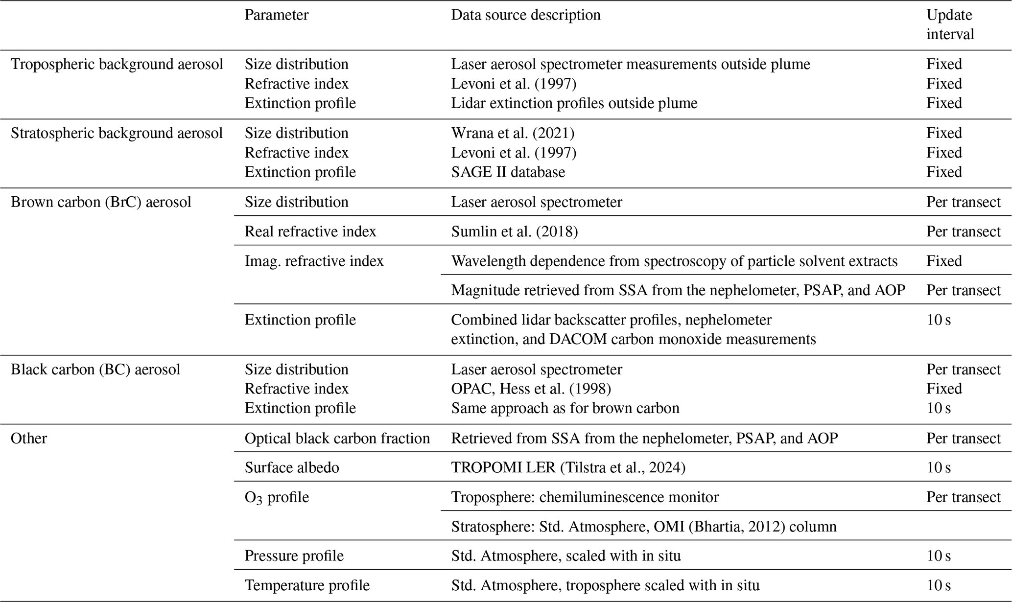
To initialize our model, the measurements introduced in Sect. 3.2 were pre-processed and combined with literature and satellite data as described in the following subsections. An overview of the input data is provided in Table 2. We use a vertical grid of 87 layers extending from the ground to 62 km above ground level (a.g.l.). The layer thickness was set to 100 m between 0 and 6 km (approximately covering the altitude range of the flight), 250 m between 6 and 9 km, 3000 m between 9 and 42 km, and 5000 m between 42 and 62 km altitude a.g.l. The spectrum by Chance and Kurucz (2010) was used for the extraterrestrial solar irradiance. All literature spectra were spectrally smoothed prior to simulation (Δλ = 2 nm) as described in Sect. 2.5, which was found to approximately match the resolution of the CAFS instrument. Full simulations were performed on an irregular wavelength grid with 23 nodes (see Sect. S2), with denser sampling towards UV wavelengths. The grid was optimized for the interpolation approach described in Sects. 2.5 and S2. The final actinic flux spectra were calculated from these simulations using the aforementioned interpolation approach with a spectral sampling interval of 0.2 nm. For the VLIDORT scattering RT solver, the number of discrete ordinate streams in the polar half-hemisphere was set to 8. In addition, the “delta-M scaling” ansatz was used to deal with sharply peaked forward-scattering characteristic of aerosols.

Spatial distributions (2D plume cross-sections) of actinic flux and photolysis frequencies are modeled for each of the 20 transects highlighted in the lower panel of Fig. 3. The horizontal resolution of the modeled distributions is determined by the speed of the aircraft and the temporal resolution at which input data are available. As indicated in Table 2, different model input parameters are updated at different temporal intervals, depending on the parameter's data availability, variability, and relevance for the RT.

1. 10 s: the temporal resolution of the model simulations is ultimately limited by the resolution of the lidar backscatter profile measurements (10 s). All model input data available at shorter time spans are therefore averaged to at least 10 s intervals prior to simulation, which corresponds to an approximate horizontal resolution of 1.5 km.

2. Per transect: for some parameters (e.g., particle filter measurements) only transect average observations exist. Other parameters (e.g., PSD) appeared to be constant over individual transects within the measurement uncertainty. Those were averaged to reduce measurement noise.

3. Fixed: for some parameters constant values are used for the entire flight, e.g., for those taken from the literature or in the case of scarce data coverage.

Levoni et al. (1997)Wrana et al. (2021)Levoni et al. (1997)Sumlin et al. (2018)Hess et al. (1998)(Tilstra et al., 2024)(Bhartia, 2012)

Table 2 Overview of the data used to constrain the model for actinic flux and photolysis frequency simulations in the Shady fire plume.

4.1 Background aerosol

Two aerosol types are used to represent tropospheric and stratospheric background aerosol, and both types are based on the microphysical model of the VPC aerosol module (Sect. 2.2.2). For stratospheric background aerosol, extinction profiles were taken from the SAGE II database (SAGE Science Team, 2012). The size distribution was adapted from Wrana et al. (2021). For the particle refractive index we assume a mixture of 75 % H₂SO₄ and 25 % water (Levoni et al., 1997), yielding a value of $\mathrm{1.43}+i\times {\mathrm{10}}^{-\mathrm{8}}$ based on Palmer and Williams (1975) and Segelstein (1981). We use the same value for all wavelengths.

For tropospheric background aerosol, the extinction profile is inferred by averaging outside-plume observations of the lidar during the flight. Similarly, outside-plume measurements from the laser aerosol spectrometer were averaged to obtain the size distribution. For the refractive index we use a constant value of $\mathrm{1.53}+i\cdot \mathrm{0.007}$, as reported for clean continental air by Levoni et al. (1997).

4.2 Plume aerosol

In the plume, we consider the two optically dominant particle compounds: black carbon (BC) and brown carbon (BrC). BC and BrC are each represented by their own aerosol type in the model. Both types use the microphysical model of the VPC aerosol module (Sect. 2.2.2), and we assume particles to be spherical and internally homogeneous. The results presented in this study indicate that the plume bulk optical properties can be sufficiently reproduced using this simplified approach, even though real morphology and mixing states of BB particles can be much more complex (see, e.g., Hand et al., 2010; Liu et al., 2021). Particle properties are assumed to be altitude-independent, as measurements performed at different altitudes with respect to the plume center did not show significant changes.

PSD parameters were inferred for each transect by averaging corresponding laser aerosol spectrometer data and fitting a bimodal lognormal distribution as accepted by the microphysical aerosol model (Sect. 2.2.2). We assume the same PSD for BrC and BC, since the laser aerosol spectrometer cannot distinguish between the aerosol types.

The refractive index for BC was taken from the OPAC database (Hess et al., 1998). We used a fixed value of $\mathrm{1.7}+i\cdot \mathrm{0.46}$ for all wavelengths. The real part of the BrC refractive index was set to a fixed value of 1.53, following Sumlin et al. (2018). The imaginary refractive index κ_BrC was inferred from SAEB measurements. The recorded SAEB spectra (Sect. 3.2) reflect the wavelength dependence of the BrC material absorption coefficient α_BrC, which can be converted to an unscaled imaginary refractive index using the relation ${\mathit{\kappa }}_{\mathrm{BrC}}\propto {\mathit{\alpha }}_{\mathrm{BrC}}\cdot \mathit{\lambda }$ (Bohren and Huffman, 1998). With the PSD and refractive index information, we set up the microphysical aerosol model for BC and BrC mixtures to simulate bulk overall SSAs. We fit these SSAs to the ones observed by the nephelometer, PSAP, and AOP measurements to retrieve the BC to BrC ratio and the magnitude of κ_BrC for each plume transect. To describe the BC to BrC ratio we introduce the “optical BC fraction”, which represents the contribution of BC to the total extinction of BC and BrC at a prescribed reference wavelength λ₀. It is used below to calculate separate vertical profiles for BrC and BC. Average retrieved values for κ_BrC and the optical BC fraction at 300 nm are on the order of 0.05 and 0.08, respectively. A typical BrC imaginary refractive index obtained this way is shown in Fig. S1. The retrieved values reproduce the plume bulk optical properties well (Sect. 5), but it should be noted that their physical meaning is limited due to the simplifications implicit in the aerosol modeling approach.

Aerosol extinction profiles were inferred from lidar, nephelometer, and DACOM data. Due to the limitations in the lidar aerosol extinction profiles (Sect. 3.2) the lidar aerosol backscatter profiles (B) had to be used to achieve suitable spatial resolution and vertical coverage. Conversion to extinction (E) was achieved by investigating aerosol lidar ratios $S=E/B$ observed during plume overflights (see Fig. 3). S was found to depend primarily on the smoke age t (see Fig. S3). This dependence was parameterized by fitting a second-order polynomial S(t), used to calculate the extinction profiles $E=S\left(t_{\text{transect}}\right)\cdot B$ for each transect. The vertical gap arising from the lidar's non-overlap region around the aircraft was filled using in situ measured extinction from the nephelometer and linear interpolation. Smaller temporal gaps in the nephelometer data were filled using carbon monoxide data from the DACOM instrument, applying a conversion factor inferred from nephelometer–DACOM correlations in the same transect (typical Pearson r correlation > 0.99). Missing data above or below the plume were either zero-padded or extrapolated assuming a Gaussian plume shape. Separation into BC and BrC contributions was made based on the current transect's optical BC fraction.

4.3 Surface reflectance

Surface reflectances are taken from the TROPOMI database for monthly Lambertian-equivalent reflectivity (LER; Tilstra et al., 2024). The database has a spatial resolution of 0.125° × 0.125° (10 km × 14 km for the Shady fire location), and its 39 spectral channels cover a wavelength range from about 330 to 2300 nm. Below 330 nm, we assume a linear decrease to zero at 250 nm. We consider these approximations to be reasonable, since the surface albedo is generally low with a minimal impact on the total actinic flux.

4.4 Trace gases

The only trace gas taken into account for our study was O₃. Based on in situ measurements performed on the aircraft, we estimated the absorption of other trace gases to be small (< 3 % in actinic flux spectra) and omitted them for simplicity. The O₃ tropospheric profile was inferred from O₃ in situ measurements on the aircraft during ascent and descent at take-off and landing. For the stratosphere we assumed the 1976 US Standard Atmosphere, scaled such that the O₃ total column matched OMI satellite observations (Bhartia, 2012).

5 Results

We ran the VPC model for the 20 transects indicated in Fig. 3. Simulation runs were performed at 10 s temporal resolution (corresponding to a horizontal spatial resolution of ≈ 1.5 km) and 100 m vertical resolution at flight altitude, roughly matching the resolution of the lidar observations (Sect. 3). For each run, the model was constrained as described in Sect. 4 based on the plume composition and vertical distribution observed at the respective time and location. In total, 350 model runs (10 to 30 runs per transect) were performed. Each run provides vertical profiles for the actinic flux and photolysis frequencies.

For the investigation of photolysis frequencies, we will focus on four important atmospheric reactions with different spectral sensitivity.

$$\begin{array}{c}{\displaystyle }{\mathrm{O}}_{\mathrm{3}}+h\mathit{\nu }\to {\mathrm{O}}_{\mathrm{2}}+\mathrm{O}{(}^{\mathrm{1}}\mathrm{D})\\ {\displaystyle }\mathrm{HONO}+h\mathit{\nu }\to \mathrm{OH}+\mathrm{NO}\\ {\displaystyle }{\mathrm{NO}}_{\mathrm{2}}+h\mathit{\nu }\to \mathrm{NO}+\mathrm{O}{(}^{\mathrm{3}}\mathrm{P})\\ {\displaystyle }{\mathrm{NO}}_{\mathrm{3}}+h\mathit{\nu }\to {\mathrm{NO}}_{\mathrm{2}}+\mathrm{O}{(}^{\mathrm{3}}\mathrm{P})\end{array}$$

Figure 4 illustrates the spectral sensitivity by showing action spectra (actinic flux spectrum × reactant absorption cross-section × quantum yield) for each reaction, assuming typical modeled actinic flux spectra with and without the plume present. The action-spectra-weighted average wavelengths for the four reactions are approximately 310, 360, 375, and 550 nm.

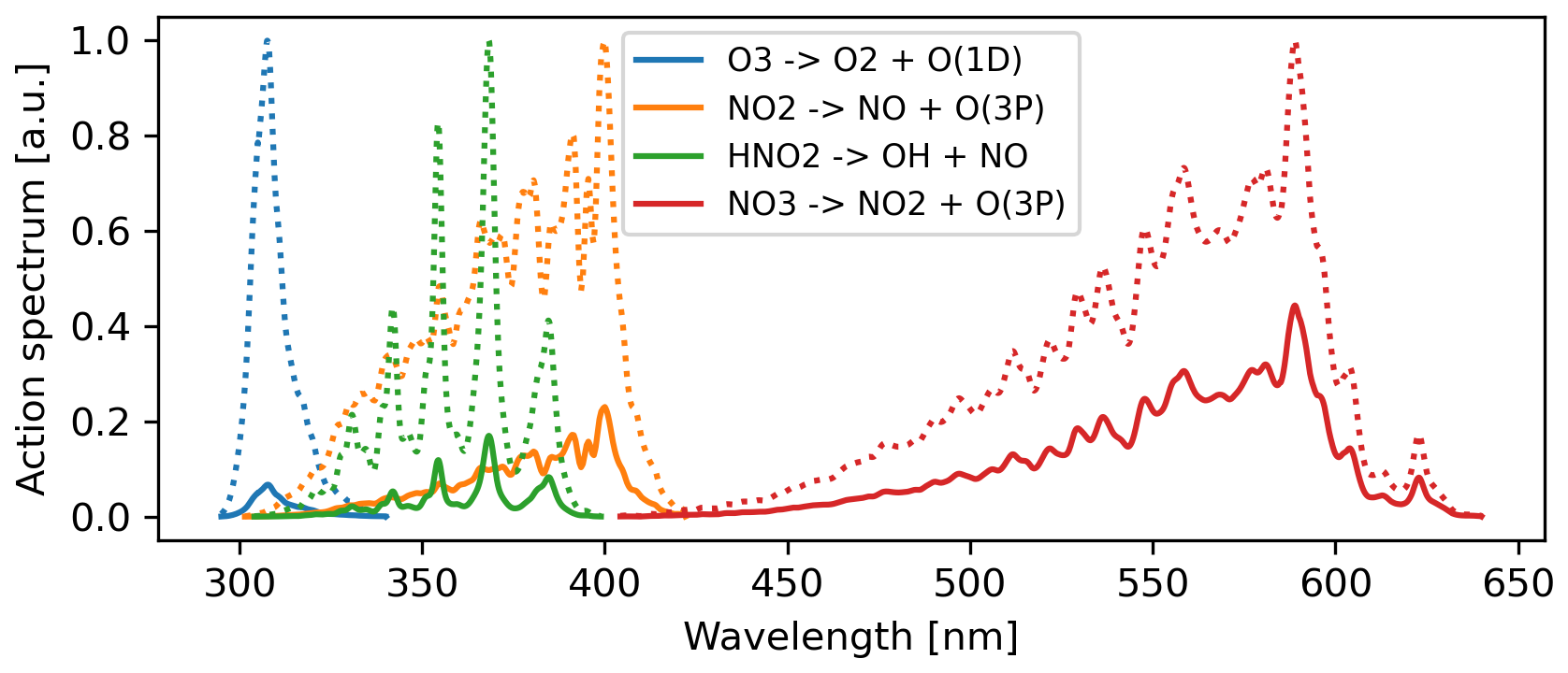
Figure 4 Spectral sensitivity of the four photochemical reactions considered in the comparison. Shown are action spectra (actinic flux × reactant absorption cross-section × quantum yield) assuming a typical tropospheric Rayleigh atmosphere actinic flux (dotted lines) or a dense plume (AOD ≈ 3 at 532 nm) actinic flux spectrum (solid lines).

5.1 General features of the BB plume environment

It is instructive to start with a discussion of general features of the BB plume environment. Figures 5 and 6 show combined overviews of modeling results and observations for four selected transects (5, 8, 14, and 20) covering different situations. Similar plots for all 20 transects can be found in Sect. S6. To provide a picture of the full wavelength range, Fig. 7 shows measured and modeled spectra for three selected model runs (as highlighted by the black rectangles in Fig. 5) with the aircraft flying within, above, and below the plume.

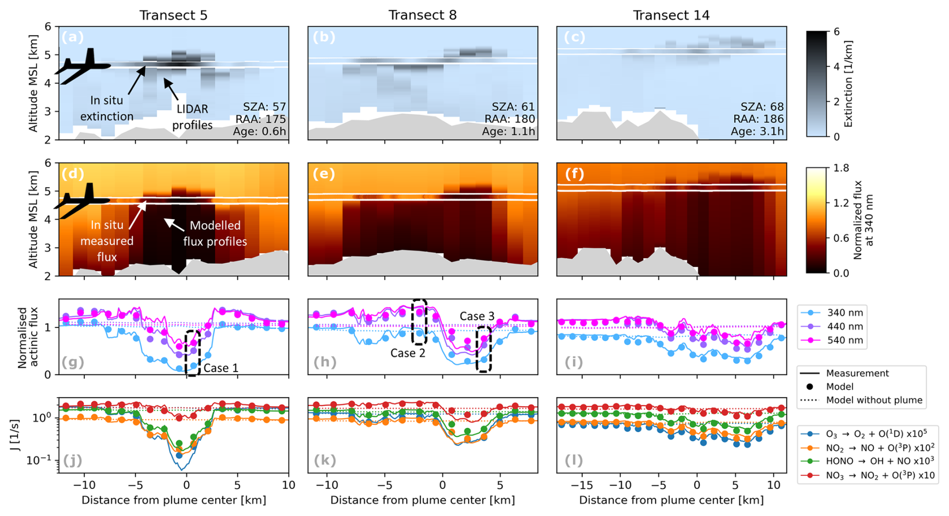
Figure 5 Overview of modeled and observed (CAFS) actinic fluxes and photolysis frequencies for three example transects. The first and second rows show plume cross-sections of measured aerosol extinction (532 nm) and modeled actinic flux, respectively. The observer is looking downwind. Solar relative azimuth angles (RAAs) are given with respect to the viewing direction: 0, 90, or 180° indicate sun in front, to the right, or to the back of the observer, respectively. Altitudes are given with respect to mean sea level (m.s.l.). The third row shows time series of in situ actinic fluxes at three wavelengths, normalized to TOA irradiance. Black rectangles indicate observations discussed in more detail throughout the paper (see also Figs. 13, 7, and 12). The fourth row shows in situ photolysis frequencies for three example reactions. For reference, dashed lines indicate Rayleigh atmosphere actinic fluxes and photolysis frequencies created by re-running the model without the plume present.

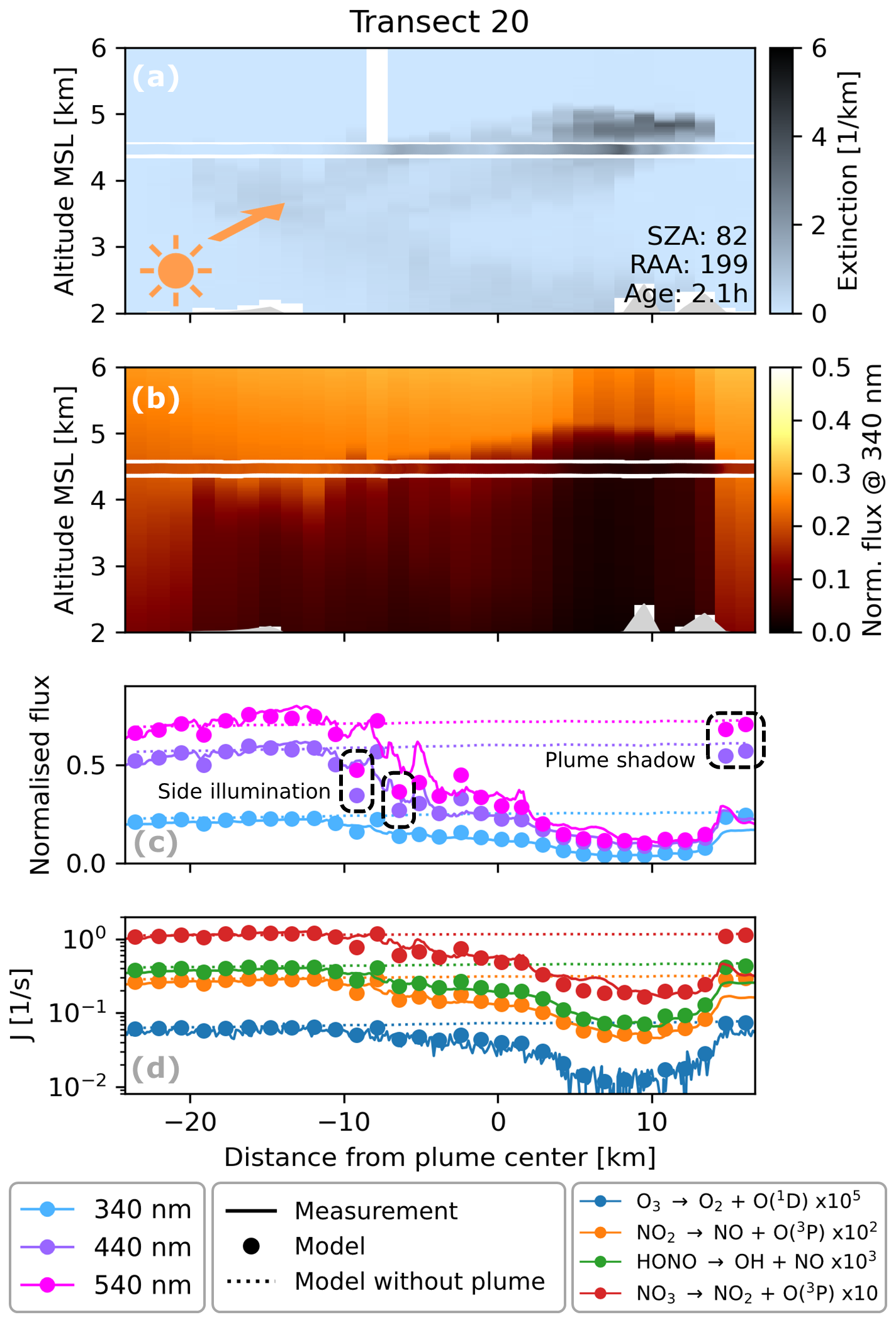
Figure 6 Example transect with a particularly high SZA (82°). The legend and description for Fig. 5 apply, but note the different scales.

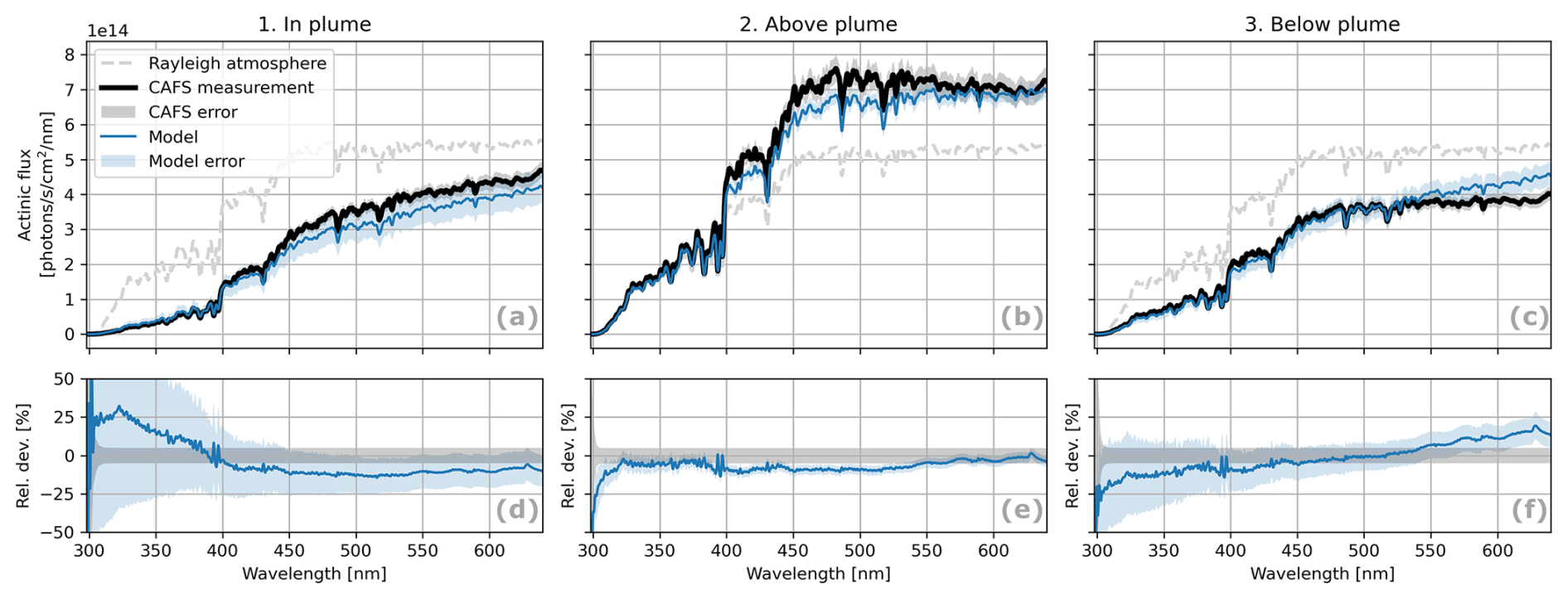
Figure 7 Modeled and measured (CAFS) actinic flux spectra for three example observations (as highlighted in Fig. 5). To put the flux magnitudes into perspective, “Rayleigh atmosphere” spectra were calculated by re-running the model without plume aerosols. The modeled spectra were interpolated between simulation nodes following the procedure described in Sect. 2.5. Model errors were estimated using the sensitivity studies described in Sect. 5.2.3 and do not consider errors from horizontal radiative transport effects. (a, b, c) Actual actinic flux spectra. (d, e, f) Relative differences between the model and measurements.

The underlying data for the selected transects were sampled at different times of the flight (compare transect labels in Fig. 3) and at different distances to the fire (20, 40, 100, and 60 km, respectively). As indicated by the 2D distributions of aerosol extinction coefficients (Figs. 5a–c and 6a), the sampled plume cross-sections have a horizontal (vertical) extent of 10 to 15 km (1 to 2 km) and are located about 2 to 3 km above the ground. Plume density and shape vary strongly between different transects. In a young and dense plume, extinction coefficients and AODs of up to 6 km⁻¹ and > 3 (both at 532 nm) are encountered, respectively (Fig. 5a). Around the vertical middle of the plume, this leads to reductions in actinic flux (Fig. 5g) and photolysis frequencies (Fig. 5j) of more than an order of magnitude compared to the clean atmosphere outside the plume. The reduction is most pronounced in the UV and UV-centered photolysis frequencies; i.e., the actinic flux at 340 nm is strongly reduced (Fig. 5g) and is near zero at wavelengths below 340 nm (Fig. 7a). The aerosol model results identify the increasing BrC absorption as the main reason (Fig. S1), rendering the plume darker and more opaque at the same time. BrC approximately triples plume aerosol extinction and reduces the SSA from 0.9 to 0.75 when comparing 532 to 300 nm. The radiative conditions above, within, and below the plume are very different and, depending on the wavelength, can lead to either enhancement or reduction in actinic flux and photolysis frequencies in comparison to the situation with a clean atmosphere. During transect 8, the relative height of the aircraft with respect to the plume varies (Fig. 5b). We see enhancements in actinic flux and photolysis frequencies (Fig. 5h and k), particularly towards Vis wavelengths, when the aircraft is above or in the upper region of the plume and a reduction in both UV and Vis when the aircraft moves deeper into or below the plume. This behavior is also apparent in the example spectra (Fig. 7) as well as the actinic flux vertical profiles (Figs. 5d–f and 6b) and will be investigated in more detail in Sect. 6.

Transect 14 represents a plume older than > 3 h. Older plumes are typically wider, more ragged, and optically thinner (Fig. 5b, c). Accordingly, the reductions in actinic flux and photolysis frequencies are less pronounced (Fig. 5i, l).

5.2 Comparison of model and measurement

In this section we compare the modeled actinic fluxes and photolysis frequencies to the ones observed by the CAFS. The comparison serves to validate the VPC model and to assess the accuracy of modeling results. While the model provides full vertical profiles of actinic flux and photolysis frequencies, the comparison is limited to a single altitude per model run, namely the altitude of the aircraft, where the respective CAFS measurement was performed. However, the dataset includes measurements at different relative altitudes with respect to the plume. We therefore expect the average agreement of the model and measurements to be representative for all modeled distributions.

5.2.1 Comparison of actinic fluxes

The qualitative agreement of the model and measurement can already be seen in the combined plots of actinic flux time series in Figs. 5g–i and 6c. The model reproduces major reductions and enhancements in the time series very well. Occasional outliers typically occur at the plume edges, particularly late in the evening (see highlighted model runs in Fig. 6c), and are discussed later (Sect. 6).

To quantify the model–measurement differences, we performed a statistical analysis. In this analysis, we compare actinic flux optical depths (AFODs), which are the logarithm of the normalized actinic flux (Eq. 6). AFODs may be less intuitive than the actinic flux itself, but their use offers several advantages: (1) AFOD root mean square deviations and linear regression results between the model and measurements provide relative instead of absolute differences. We found relative differences to be less dependent on the actinic flux magnitude and therefore to be more representative for the full dataset. (2) Especially in dense BB plumes, a linear approach would give more weight to higher actinic fluxes, which are found outside of the plume, thus leading to improper characterization of the RT in the center of the plume. (3) Because the actinic flux varies by over an order of magnitude, a logarithmic scale will more evenly represent the agreement over the large variation of the actinic flux and is less sensitive to outliers. (4) The AFOD increases with the plume signal and for high SZAs. In this way, the linear regression offset approximately represents the model–measurement differences in clean air during daytime, and the slope reflects systematic errors increasing with aerosol signal (e.g., errors in the aerosol representation or properties) and twilight conditions. This enables a more direct analysis of the RT effects inside the plume.

Figure 8 Correlation plots of measured (CAFS) and modeled (VPC) actinic flux optical density (AFOD; see Eq. 6). Data points in the plot are limited to the same wavelengths (340, 440, and 550 nm) as shown in Fig. 5. For the difference histogram and linear regression results on the right, the whole dataset was considered.

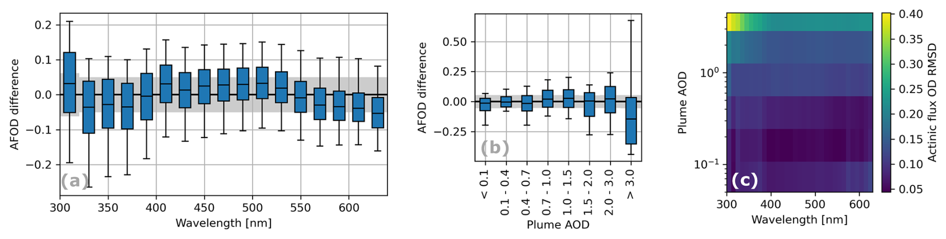
Figure 9 Agreement of modeled and measured actinic flux optical density (AFOD) as a function of wavelength and plume total AOD. AODs were calculated from lidar observations at 532 nm. Boxes span the 25th to 75th percentile. Whiskers span the 10th to 90th percentile. Gray shaded areas show average CAFS measurement uncertainty.

To quantify the overall agreement of the model and observations, we performed a correlation analysis on the entire dataset (Fig. 8), including all 20 transects, all wavelengths, and also locations outside the plume. CAFS observations – with an original temporal resolution of 1 s – were averaged over each of the modeled 10 s time intervals. We applied two filters: (1) we only considered data for which the CAFS signal-to-noise ratio is higher than 5 (removes < 2 % of the data), and (2) we subsequently ignored the highest first percentile of differences to remove the most severe outliers, which are mostly associated with inhomogeneities in the plume not captured by the model. Based on these data, we obtain a Pearson correlation coefficient of 0.98 between the model and measurements. The RMSD in AFOD is 0.17, which corresponds to a 17 % deviation in the actinic flux. The slope (0.98) and intercept (−0.004) from the linear regression analysis indicate no significant systematic differences. As described in Sects. 2.4 and 3.3, both CAFS and VPC provide upwelling and downwelling actinic flux contributions separately. Correlation analysis results for each of the contributions are provided in Sect. S4. The upwelling part exhibits larger deviations (RMSD of 24 %) than those for the downwelling part (RMSD of 17 %), which is most likely due to imperfect representation of surface properties, surface illumination (e.g., shadowing by the plume), and the assumption of constant ground elevation in the model. However, the impact of this increased deviation is limited, since in the presented data, upwelling radiation contributes on average only ≈ 20 % to the total actinic flux.

To obtain a more differentiated picture, we investigated the dependence of model–measurement differences on wavelength, plume AOD, and solar geometry by binning the data (Figs. 9 and 10). For the AOD binning, we used the AODs at 532 nm observed by the lidar. Overall, we found this AOD to be a good proxy to identify observations significantly affected by the presence of the plume, even though the impact of the plume signal also depends on the aircraft's altitude with respect to the plume. We find a clear increase in model–measurement difference towards short wavelengths (Fig. 9a and also Fig. 7) and high AODs (Fig. 9b). For wavelengths > 400 nm and low AODs, RMSDs of 0.05 to 0.1 are observed. In contrast, for wavelengths around ≈ 300 nm and high AODs (≈ 4 at 532 nm and ≈ 10 at 300 nm), RMSDs increase up to 0.4 (Fig. 9c). At high AODs, Fig. 9b indicates a general systematic underestimation. Only observations above and in the upper plume contribute to this data bin, since observations below do not meet the CAFS signal-to-noise filtering criterion mentioned before. For intermediate AODs (1 < AOD < 3 at 532 nm), including all wavelengths, the RMSD is 0.18. We consider this value to be representative for the typical in-plume model accuracy.

For the dependence on the solar geometry, we chose three segments of the flight (transects 1, 2, and 3; transects 6, 7, and 8; transects 18, 19, and 20) with different solar geometries but otherwise similar conditions (Fig. 10a). During the first and third segment, the sun illuminates the plume from the side (albeit at a small relative azimuth angle of ≈ 15°) with respect to the plume axis) at low (≈ 50°) and high SZA (≈ 80°), respectively. During the second segment, the sun is approximately aligned with the plume axis at a moderate SZA (≈ 60°). During side illumination, in particular at high SZAs, model–measurement differences increase and model results underestimate actinic fluxes (Fig. 10b). Compared to the second segment, the RMSD for the third segment almost doubles (from 0.13 to 0.24). As discussed in detail in Sect. 6, this might be caused by the 1D model assumption of a horizontally homogeneous atmosphere.

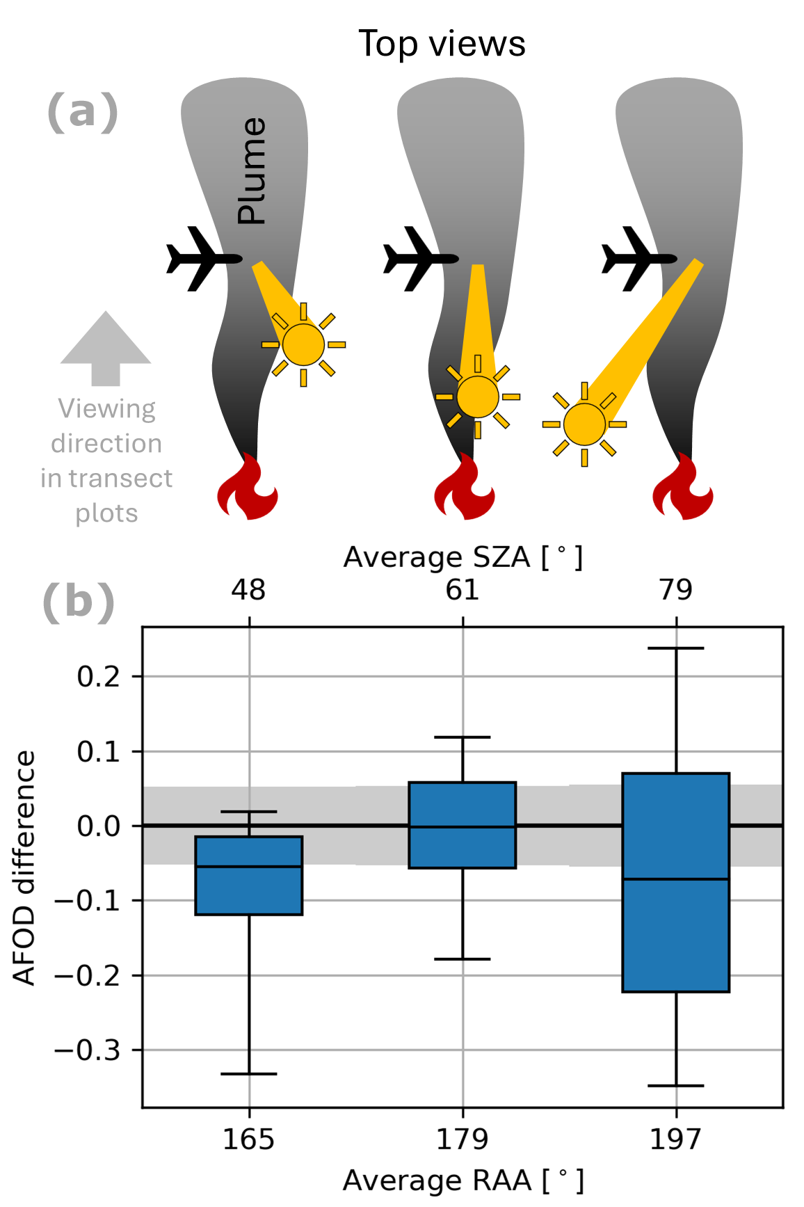
Figure 10 (b) Agreement of the model and measurement for three segments of the measurement flight with different solar geometries, as illustrated in panel (a). RAAs were calculated with respect to the plume axis, i.e., the prevalent wind direction. Boxes span the 25th to 75th percentile. Whiskers span the 10th to 90th percentile. Gray shaded areas show average CAFS measurement uncertainty.

5.2.2 Comparison of photolysis frequencies

From a chemical point of view, it is interesting to assess how the model–measurement differences in actinic fluxes propagate into the photolysis frequencies. We therefore performed correlation and regression analyses similar to those in Fig. 8 for the modeled and measured photolysis frequencies of the 48 tropospheric photochemical reactions already mentioned in Sect. 2.4. Again, the first percentile of data with the highest differences were omitted. Results for the four reactions introduced at the beginning of Sect. 5 are shown in Fig. 11. The results for the remaining reactions are listed in Sect. S2. Note that, instead of the root mean square of absolute deviations (RMSDs), we calculate the root mean square of relative deviations (RMSRDs) here, according to

$$\begin{array}{}\text{(9)}& \text{RMSRD}=\sqrt{{\displaystyle \frac{\mathrm{1}}{N}}\sum _{i=\mathrm{1}}^N{\left({\displaystyle \frac{y_i-x_i}{x_i}}\right)}^{\mathrm{2}}},\end{array}$$

with x_i and y_i being measured and observed photolysis frequencies, respectively. This facilitates the comparison between different reactions.

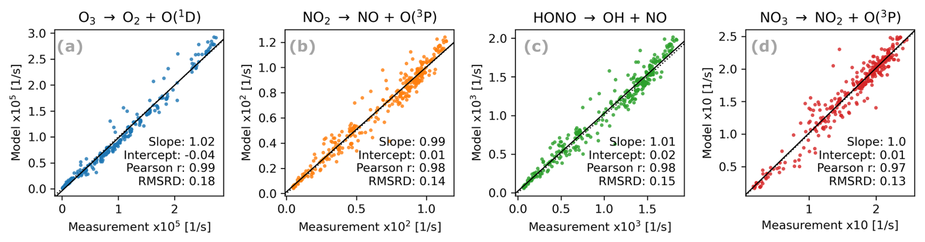
Figure 11 Agreement of modeled and measured photolysis frequencies for the four example reactions with different spectral sensitivity. Instead of root mean squares of absolute differences, we show root mean square values of relative differences here (RMSRDs) for easier comparison of different reactions.

As mentioned before, CAFS and VPC use the same photolysis frequency code, quantum yield, and absorption cross-section data. The conversion from actinic fluxes to photolysis frequencies therefore does not introduce additional differences between model and measurement; photolysis frequencies simply reflect the actinic flux differences, weighted by the action spectrum of the corresponding reaction (Fig. 4). Accordingly, systematic differences (slope and offset of the linear regressions) and RMSRDs for the photolysis frequencies are similar to those obtained for actinic fluxes and follow the patterns already seen in Fig. 9a. Larger differences are found for UV-driven reactions like O₃ photolysis (Fig. 11a). Smaller differences are observed for Vis-driven reactions, especially NO₃ photolysis (Fig. 11d), which also benefits from integration over a broad spectral range (see action spectrum in Fig. 4). For all 48 reactions, Pearson correlation coefficients are > 0.96, slopes are between 0.96 and 1.04, and intercepts range between −5 % and +2 % of the average observed photolysis frequency for the respective reaction (Sect. S2). RMSRDs are between 0.12 and 0.21, with an average of 0.15.

5.2.3 Model sensitivity to input parameters

To better understand the origin of the model–measurement differences and identify critical factors, we performed model sensitivity studies; i.e., we investigated the response of the modeling results to variations in the input parameters.

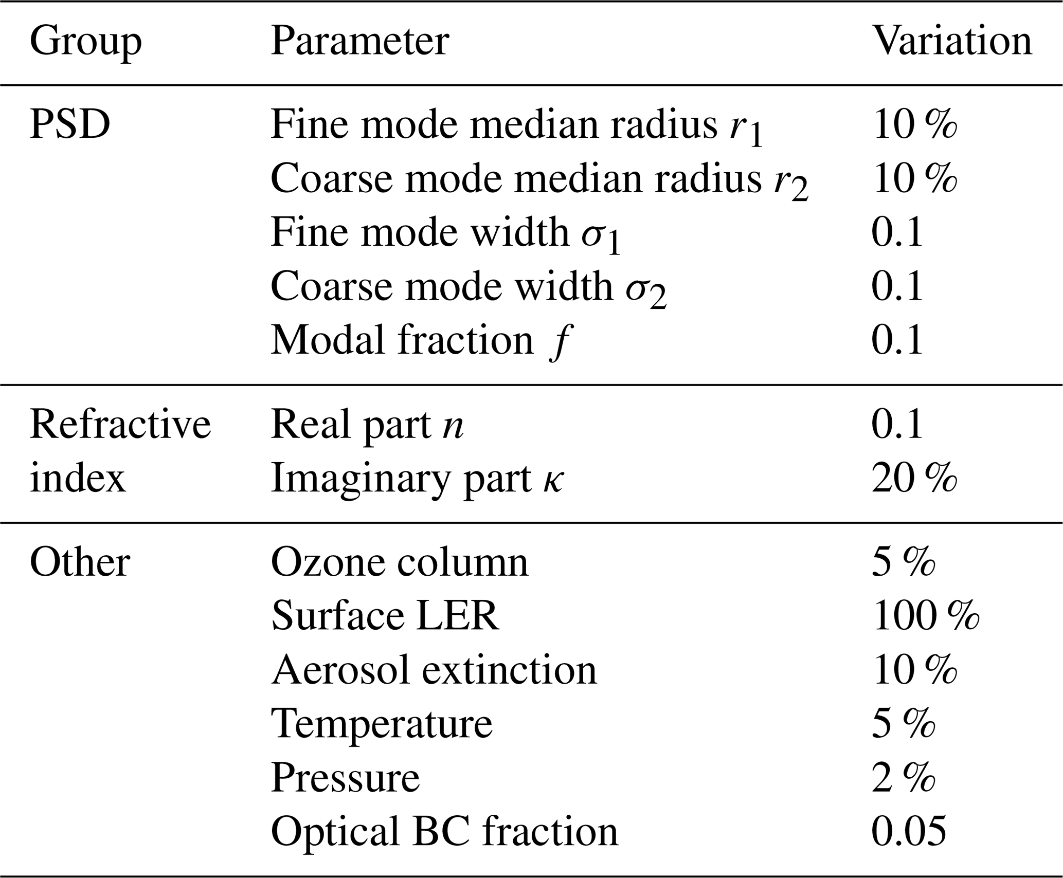
The variations applied to the model inputs are listed in Table 3. Their magnitudes correspond to the approximate uncertainties in the respective parameter. Variations of PSD parameters, pressure, and temperature were estimated based on specifications of the corresponding FIREX-AQ instruments, but also considering noise, variability, and limited coverage of the measurements. Refractive index and optical BC fraction variations are based on the variability reported in the literature (Sarpong et al., 2020; Lack et al., 2012; Andreae and Gelencser, 2006) and from uncertainties in SSA measurements, propagated through the Mie model fit described in Sect. 4.2. O₃ column and surface LER variations are based on reported uncertainties in the corresponding satellite measurements (Shavrina et al., 2007; Balis et al., 2007; Kroon et al., 2008; Frith et al., 2020; Tilstra et al., 2024). Aerosol extinction uncertainty was assumed to be dominated by uncertainties in the lidar ratio, which we calculated from the scattering in Fig. S3. The listed variations were applied to the three simulated cases highlighted in Fig. 5 and shown in Fig. 7.

Table 3 Parameter variation magnitudes.

The resulting differences in the modeling results (Fig. 12), including their spectral dependencies, exhibit very similar magnitudes and patterns as the differences between the model and measurements reported in Sect. 5.2.1. Most parameters induce a spectrally smooth difference in the actinic flux, which increases significantly towards the UV (Fig. 12a and b). Furthermore, the differences increase with the plume AOD; i.e., they are largest (with a total of up to 60 % in the UV) inside the optically dense plume of transect 5 (Fig. 12a) and become smaller (up to 40 %) for the thinner plume encountered during transect 8 (Fig. 12c). The smallest differences are found above the plume (Fig. 12b). Here, the actinic flux is dominated by the contribution from direct solar radiation (see also Fig. 13), which is not affected by plume aerosols but is prone to uncertainties in the stratospheric O₃ column below 315 nm.

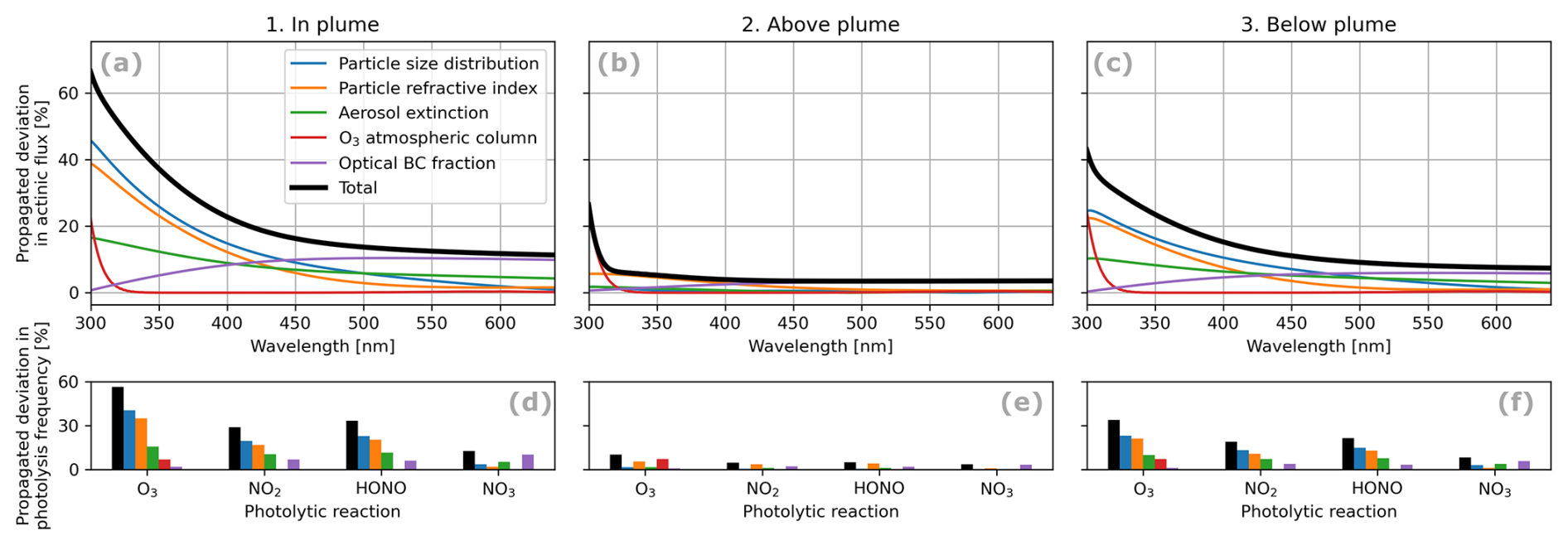
Figure 12 Response of actinic flux spectra (a, b, c) and photolysis frequencies (d, e, f) to the parameter variations defined in Table 3 for the three example spectra presented in Fig. 7. Parameters have been grouped here for readability by quadratically adding their propagated impact. The legend in panel (a) applies to the entire figure.

In and below the plume, uncertainties in the UV are dominated by particle properties such as refractive indices and the PSD. Investigating the contributions of separate parameters and aerosol types (not shown in Fig. 12) provides further insights: as expected from the generally low optical BC fraction (10 % at around 500 nm) and the strong increase in BrC absorption towards the UV, these uncertainties are dominated by the BrC properties, while BC parameter variations contribute less than 20 % to the total uncertainty below 350 nm.

In the Vis, uncertainties are generally lower than those in the UV, since plume optical thickness decreases with wavelength. The uncertainty is dominated by the optical BC fraction, which is approximately proportional to the plume extinction. The contribution from BrC becomes negligible towards longer wavelengths.

6 Discussion

The major features in the observed actinic flux and photolysis frequency time series (Figs. 5 and 6), as well as in the actinic flux spectra (Fig. 7), are well-reproduced by the model. RMSDs over the entire dataset are on the order of 10 % to 20 % in both actinic fluxes and photolysis frequencies. Systematic differences in our comparison are on the order of a few percent, as illustrated by the regression slope of 0.98 and negligible intercept between measured and modeled actinic fluxes (Fig. 8) as well as slopes between 0.99 and 1.02 in the measured and modeled photolysis rates (Fig. 11). These differences are smaller than the uncertainty in the CAFS measurements (Figs. 8, 9, 11).

Generally we find surprisingly good model–measurement agreement, considering the complexity, heterogeneity, and variability of BB plumes and the large variations in actinic flux and photolysis frequencies over more than an order of magnitude on short spatial and temporal scales. To put our results into perspective, similar airborne (Kelley et al., 1995; Volz-Thomas et al., 1996) and ground-based (Barnard et al., 2004; Castro et al., 1997; Dickerson et al., 1997; Kazantzidis et al., 2001; Vuilleumier et al., 2001; Balis et al., 2002; Shetter et al., 2003; Hofzumahaus et al., 2004) model–measurement comparisons for less polluted and nearly homogeneous clear-sky atmospheres typically achieve agreement on the order of 10 %.

Besides the relatively small CAFS measurement error, model–measurement differences arise for two major reasons: errors in the model input parameters and simplifications taken in the modeling approach.

Errors in model input parameters partly arise from instrumental measurement errors and uncertainties in the literature data that were used to constrain the model (Sect. 4). Furthermore, the limited spatiotemporal coverage and limited resolution of these data do not fully encompass real variations in the inhomogeneous plume, thereby adding considerable uncertainty to the model constraints. Nonlinear relations between plume properties and actinic fluxes might also hinder exact simulations when using averaged parameters.

Model simplifications are the representation of aerosol (as spherical particulates and externally mixed) and the application of a 1D model, which cannot account for horizontal RT effects. The latter are caused by the horizontal inhomogeneities of the scenario. Such effects comprise, for instance, side illumination and shadowing, especially at the edges of the plumes. But also on smaller scales and within the plume, horizontal RT can affect the results. For instance, the fact that the lidar aerosol extinction profile was measured in the zenith direction, while the RT calculation was performed for nonzero SZA can introduce inconsistencies in the aerosol extinction profiles.

For our sensitivity studies (Sect. 5.2.3), we estimated the uncertainties in the model input parameters, considering both instrumental errors and uncertainties due to limited coverage and resolution of the measurements. Propagating these uncertainties through the model yields model uncertainties very similar to the observed model–measurement differences, not only in magnitude but also in wavelength and AOD dependence (compare Figs. 9 and 12). We conclude that, at least as average behavior over the dataset, the model–measurement differences are dominated by uncertainties in the model input. Hence, even with comprehensive state-of-the-art measurements as performed during FIREX-AQ, the information on the plume environment is still the limiting factor for accurate modeling of actinic fluxes and photolysis frequencies in BB plumes. Most critical is the uncertainty in brown carbon aerosol properties (refractive indices and PSD), which dominates the model uncertainties in the UV (Fig. 12), where photochemistry is most sensitive. BrC properties are difficult to assess as they are highly variable and the mechanisms affecting the absorption's spectral dependence are not yet fully understood (e.g., Laskin et al., 2015; Shetty et al., 2023). A recent comparison study revealed inconsistencies between different approaches to derive BrC optical properties from FIREX-AQ data (Zeng et al., 2022), presumably in part due to insoluble BrC components that the SAEB technique (Sect. 3) cannot detect (Liu et al., 2013; Shetty et al., 2019; Chakrabarty et al., 2023). In our study, this effect is likely reduced, since we combine the SAEB observations with direct in situ optical measurements of the SSA (Sect. 4.2). However, the absence of SSA observations in the UV and the inhomogeneity of the plume hinder an accurate consideration of BrC in the modeling process. We propose that further investigation of the discrepancies between in situ extractive BrC sampling and remotely sensed actinic flux or radiance spectra may shed light on this issue and ultimately better constrain radiative transport and photochemistry in BB plumes.

Considering that most of the model–measurement differences can be explained by uncertainties in the model input, simplifications in the model are unlikely to limit the modeling accuracy under typical conditions. However, horizontal radiative transport effects might become problematic for specific cases. These effects – in particular side illumination and shadowing – are expected to be most pronounced when the SAA is not aligned with the plume axis, i.e., the sun illuminates the plume from the side (first and third sketch in Fig. 10a), and when SZAs are large. Indeed, we observe a dependence in model–measurement differences, matching these expectations (Fig. 10b). Furthermore, horizontal radiative transport effects are likely to occur at the plume edges, where horizontal inhomogeneity is large. An extreme case, where all three conditions are fulfilled, is represented by the plume edges of transect 20. The actinic flux time series indicates strong underestimations and overestimations (black boxes in Fig. 6c), which can be explained by plume side illumination and shadowing, respectively. It should be noted that the Shady fire dataset is favorable in this context, since the sun is almost aligned with the plume axis over the entire flight (Sect. 3). Plumes under less favorable geometries might lead to larger horizontal radiative transport effects. On the other hand, corrections, for example based on additional measurements of direct solar AOD, might reduce these effects in the future (Várnai and Davies, 1999).

With the confidence that we can model actinic fluxes and photolysis frequencies accurately, it is worth discussing the modeled spatial distributions of actinic fluxes and photolysis frequencies. Figure 13 shows actinic flux vertical profiles for case 1 during transect 5 (black box in Fig. 5g). We separated contributions from direct, diffuse downwelling, and diffuse upwelling flux and investigated two wavelengths close to the lower and upper end of the photochemically relevant wavelength range (320 and 600 nm in panels a and b, respectively). For the wavelengths in between these values, the profiles were found to transition steadily into each other.

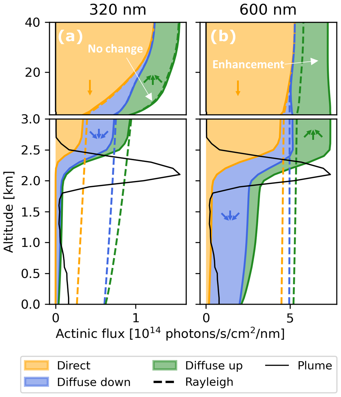
Figure 13 Detailed plot of the simulated actinic flux vertical profile for case 1 in transect 5 (black box in Fig. 5g) in the UV (a) and Vis (b). Colored areas indicate separate contributions from direct as well as diffuse upwelling and downwelling radiation. The thin black line indicates the plume extinction profile in arbitrary units. Note the different altitude scales of the upper and lower panels. To put fluxes into perspective, dashed lines show results for a Rayleigh atmosphere without a plume.

Below the plume, the contribution from direct sunlight is considerably reduced in the UV and Vis, leading to a net reduction in the actinic fluxes, despite the enhancement of the diffusive radiation fields (e.g., the Vis downwelling contribution in Fig. 13b). Above the plume, the behavior is very different for UV and Vis. In the Vis (Fig. 13b), more light is scattered upwards, as the plume albedo is larger than the typically dark Earth surface (LER ≲ 10 %). This leads to an enhancement of the Vis diffuse upwelling flux on the order of 20 % for the example in Fig. 13b and up to 60 % over other parts of the Shady fire. The enhancement decreases only slightly with altitude for the infinitely horizontally extended plume in our 1D model. This behavior is very similar to the one reported for cloud layers, which are known to have substantially (> 100 %) increased (decreased) actinic fluxes and photolysis frequencies above (below) the clouds (e.g., van Weele and Duynkerke, 1993; Lefer et al., 2003).

This behavior changes significantly in the UV. While upwelling radiation from clouds is similar in the UV and Vis spectral range, actinic fluxes above BB plumes remain similar to those in a pure Rayleigh atmosphere. This is due to increased darkening of the plume by BrC absorption. For wavelengths below 320 nm, actinic fluxes above the plume are even reduced by a few percent (light gray shading above the plume in Fig. 14b), indicating that the plume appears even darker than the combined reflectance of the surface and atmosphere in a clean atmosphere. Within and below the plume the shape of the profile is similar for UV and Vis, but reductions are much stronger in the UV.

Figure 14 2D distributions of three photolysis frequencies (b, c, d) for the transect 5 plume cross-section. To illustrate the situation, panel (a) shows the plume shape in terms of aerosol extinction (same as Fig. 5a). “Enhancement factors” represent the ratio of modeled photolysis frequencies with and without a plume.

For chemical studies, the spatial distribution of photolysis frequencies in the plume is of most interest. Figure 14 shows such distributions, as obtained from the VPC model based on data from transect 5. The distributions mostly reflect the findings on the actinic flux vertical profiles. Photolysis frequencies for UV-driven reactions such as O₃ photolysis (Fig. 14b) remain unchanged (or are slightly lower) above the plume and drop to near zero towards the center or bottom of the plume. For Vis-driven reactions like NO₃ photolysis (Fig. 14d), photolysis frequencies are enhanced by up to 40 % above the plume, while the reduction within and below the plume by up to 60 % is much weaker than that in the UV. The ultimate impact of these spatial and spectral features on the plume processing should be investigated with high-resolution chemical models in the future.

7 Conclusions

We have introduced and validated VPC, a VLIDORT-based quasi-spherical 1D RT model. VPC can calculate radiances, radiative fluxes, and photolysis frequencies for a wide range of atmospheric conditions, including high loads of complex aerosol mixtures as they occur in BB or other plumes. VPC also efficiently calculates Jacobians of the simulated quantities with respect to the input parameters, facilitating its use as a forward model in remote sensing retrievals or similar inversion problems.

We have constrained the model by a comprehensive set of aerosol measurements performed during FIREX-AQ and calculated actinic fluxes and photolysis frequencies in BB plumes with an accuracy of 10 %–20 % compared to direct measurements. Previous model–measurement comparisons in clean atmospheres have found differences of < 10 %. Considering the highly complex and inhomogeneous RT environment in dense BB plumes, the agreement between VPC and the observations is remarkably good. The average difference of actinic fluxes over the entire dataset is 17 %, with larger values (≈ 40 %) at ≈ 300 nm and for large plume AODs (≈ 10 at 300 nm). For the resulting photolysis frequencies, RMSRDs range between 13 % and 21 %, with lower (higher) errors for Vis-driven (UV-driven) reactions. A further analysis of the comparison results shows very small systematic differences on the order of ≈ ±2 % between the model and the observations. Our sensitivity studies suggest that most of the RMSD can be explained by the uncertainties in the model input data, mostly arising from the limited spatiotemporal coverage and resolution of the corresponding measurements. In the UV, the model error is dominated by the uncertainty in the properties of the strongly absorbing BrC. These uncertainties can stem from the variability of refractive indexes as well as size distribution inside the plume. In the Vis, the amount and properties of black carbon dominate the model error. Due to the decrease in both strong BrC absorption and plume optical density towards the Vis, the model error in the Vis is lower by about a factor of 3 compared to the error in the UV. Given these findings and considering that photochemistry is particularly sensitive to the UV spectral range, more research on BrC optical properties in BB plumes is needed to better constrain radiative transport and photochemistry in BB plumes.

The model–measurement comparison also provides insights into the potential limitations of the 1D approximation in the RT simulations. We observe a systematic increase in the model–measurement difference by a factor of 2 for solar geometries with high SZA and when the SAA is not aligned with the plume direction. In addition, occasional outliers at the plume edges, where horizontal gradients of environmental parameters are largest, can be identified. Both of these considerations indicate that, under certain conditions, 3D RT effects can have a significant impact.

The model results also provide insights on how photochemistry is affected within and in proximity to BB plumes. Despite the absorption of BC, BB plumes appear bright in the nadir at the visible wavelength compared to the typical Earth surface. Accordingly, the additional upward-reflected light leads to enhancements of actinic fluxes in the Vis above the BB plume of up to ≈ 60 % compared to fluxes in a Rayleigh atmosphere. This enhancement can reach the upper troposphere and the stratosphere and resembles the impact of clouds on actinic fluxes reported in previous studies. However, the increase in BrC absorption significantly darkens the BB plume towards the UV. Consequently, the observed above-plume enhancement gradually disappears towards shorter wavelengths and actinic fluxes can even be reduced compared to fluxes in a Rayleigh atmosphere for wavelengths ≲ 310 nm. Inside the plume, actinic fluxes steadily decrease from top to bottom and remain approximately constant in the atmosphere below. The decrease is more pronounced in the UV than in the Vis.

Our results show good agreement between observations and measurements in the Shady fire. However, our results also highlight the challenges in describing actinic fluxes in complex dense BB plumes. The Shady fire has been selected for its favorable conditions, such as the large plume size, clear-sky conditions, comprehensive sampling, and the alignment of the sun with the plume axis. An expansion of our analysis to other FIREX-AQ plumes would allow assessment of actinic fluxes and RT modeling challenges in a wider variety of BB plumes. From the 90 fires sampled during FIREX-AQ, about five other fires provide similarly favorable conditions. Prevailing challenges for the study of other fires are scarce sampling and the presence of clouds. Identifying the most critical unknowns from additional sensitivity studies might be of great value in the future to constrain actinic fluxes in and around BB plumes with fewer measurements and less effort.

The availability of a linearized RT model, such as VLIDORT-QS, together with our sensitivity results also opens the opportunity to use actinic flux and other remote sensing observations to study aerosol optical properties. The increasing disagreement of measured and modeled actinic fluxes towards lower wavelengths strongly implies that the BrC optical properties from the in situ SAEB observations may not fully represent the true properties of the plume aerosol. The next application for VLIDORT-QS is to retrieve BrC aerosol optical properties from the measured actinic flux spectra.

Further applications are conceivable in the context of chemical transport models (CTMs). To improve computational efficiency, CTMs typically run at relatively coarse spatial resolution (several kilometers) and resort to simplifications (e.g., 1D RT modeling) and parameterizations to account for photochemical processes. Detailed modeling based on accurate measurements of the atmospheric state, similarly as presented in this study, can help us to understand the magnitudes and origins of the uncertainties introduced into CTMs by these approximations.

Adding the capacity to calculate actinic fluxes to VLIDORT-QS allows us to improve trace gas remote sensing retrievals of BB plumes. These retrievals depend on the trace gas vertical concentrations profiles, which for many of the target gases, such as O₃, NO₂, HCHO, and HONO, depend on the vertical profiles of the respective photolysis frequencies. By combining actinic flux profiles from VLIDORT-QS with a CTM, self-consistent retrievals of trace gases should be possible.

Appendix A: Abbreviations

AFOD	Actinic flux optical depth
AOD	Aerosol optical depth
BB	Biomass burning
BC	Black carbon
BrC	Brown carbon
CAFS	Charged-coupled device actinic flux spectroradiometer
CTM	Chemical transport model
FWHM	Full width at half maximum
PSD	Particle size distribution
RAA	Solar relative azimuth angle
RMSD	Root mean square deviation
RMSRD	Root mean square of relative deviation
RT	Radiative transfer
SAA	Solar azimuth angle
SAEB	Spectral analysis of extracted BrC chromophores
SSA	Single-scattering albedo
SZA	Solar zenith angle
UV	Ultraviolet (spectral range)
Vis	Visible (spectral range)
VPC	VLIDORT for photochemistry