Diurnal, seasonal, and interannual variations in δ(¹⁸O) of atmospheric O₂ and its application to evaluate natural and anthropogenic changes in oxygen, carbon, and water cycles

Variations in the δ(¹⁸O) of atmospheric O₂, δ_atm(¹⁸O), are an indicator of biological and water processes associated with the Dole–Morita effect (DME). The DME and its variations have been observed in ice cores for paleoclimate studies; however, variations in present-day δ_atm(¹⁸O) have never been detected so far. Here, we present diurnal, seasonal, and interannual variations of δ_atm(¹⁸O) based on observations at a surface site in central Japan. The average diurnal δ_atm(¹⁸O) cycle reached a minimum during the daytime, and its amplitude was larger in summer than in winter. We found that use of δ_atm(¹⁸O) enabled separation of variations of atmospheric δ(${\mathrm{O}}_{\mathrm{2}}/{\mathrm{N}}_{\mathrm{2}}$) into contributions from biological activities and fossil fuel combustion. The average seasonal δ_atm(¹⁸O) cycle reached at a minimum in summer, and the peak-to-peak amplitude was about 2 per meg (1 per meg is 0.001 ‰). A box model that incorporated biological and water processes reproduced the general characteristics of the observed diurnal and seasonal cycles. A slight but significant secular increase in δ_atm(¹⁸O) by (0.22 ± 0.14) per meg a⁻¹ occurred during 2013–2022. Secular changes in δ_atm(¹⁸O) were also simulated by using the box model considering long-term changes in terrestrial gross primary production (GPP), photorespiration, and δ(¹⁸O) of leaf water (δ_LW(¹⁸O)). We calculated changes in δ_LW(¹⁸O) using a state-of-the-art, three-dimensional model, MIROC5-iso. The observed secular increase in δ_atm(¹⁸O) was reproduced by the box model that incorporated the isotopic effects associated with the DME from Bender et al. (1994), while the simulated δ_atm(¹⁸O) showed a secular decrease when the model incorporated the isotopic effects from Luz and Barkan (2011). Therefore, long-term observations of δ_atm(¹⁸O) and better understanding of the DME are indispensable for an application of δ_atm(¹⁸O) to constrain long-term changes in global GPP and photorespiration.

1 Introduction

The ${}^{\mathrm{18}}\mathrm{O}{/}^{\mathrm{16}}\mathrm{O}$ ratio of atmospheric O₂, δ_atm(¹⁸O), is about 24 ‰ higher than that of ocean water (per definition 0 ‰ according to Vienna Standard Mean Ocean Water – VSMOW) due to various processes in the global oxygen and water cycle (e.g., Craig, 1961; Barkan and Luz, 2005). The enrichment of δ_atm(¹⁸O) is well known as the Dole–Morita effect (DME) (Dole, 1935; Morita, 1935). The DME is determined from the balance between enrichment of δ_atm(¹⁸O) due to discrimination against ¹⁸O during terrestrial and marine respiratory O₂ consumption and the terrestrial and marine photosynthetic O₂ flux, for which the δ(¹⁸O) is close to that of ocean water. Bender et al. (1994) (hereafter referred to as “B94”) reported that the isotopic effects of dark respiration, photorespiration, and the Mehler reaction associated with terrestrial respiration are 18 ‰, 21.2 ‰, and 15.1 ‰, respectively, and the terrestrial photosynthetic O₂ flux is also affected by discrimination against ¹⁸O during evapotranspiration (4.4 ‰) (see Table 1 of B94 for a summary of the isotopic effects related to the DME). Luz and Barkan (2011) (hereafter referred to as “L&B11”) also reported the isotopic effects of dark respiration, photorespiration, and evapotranspiration to be 15.8 ‰, 22 ‰, and 6.5 ‰, respectively. The DME is a useful tool for examining Earth system models because it integrates land and ocean biological and climatic components (e.g., Bender et al., 1994; Luz et al., 1999; Angert et al., 2001, 2003; Hoffmann et al., 2004; Barkan and Luz, 2005; Severinghaus et al., 2009; Luz and Barkan, 2011). Some paleoclimate studies have focused on the temporal changes in δ_atm(¹⁸O). B94 have reported that the DME is on average lower by 0.05 ‰ than that of air during the past 130 000 years, and the standard deviation of the DME from the average was ±0.2 ‰. They suggested that the DME was nearly unchanged between glacial maxima and interglacial periods, and the variability is small and may be due to variations of the relative rates of primary production on the land and in the ocean. Severinghaus et al. (2009) reported the δ_atm(¹⁸O) in the Siple Dome ice core, Antarctica, and have found that its variations over the past 60 kyr are related to Heinrich and Dansgaard–Oeschger events. They have suggested that the DME is primarily governed by the strength of the Asian and North African monsoons and have confirmed that widespread changes in low-latitude terrestrial rainfall accompany abrupt climate changes.

Table 1 Budgets and isotopic effects of the atmospheric O₂ used in the box model. Isotopic values of the external sources and DME are described versus VSMOW. B94 and L&B11 denote Bender et al. (1994) and Luz and Barkan (2011), respectively.

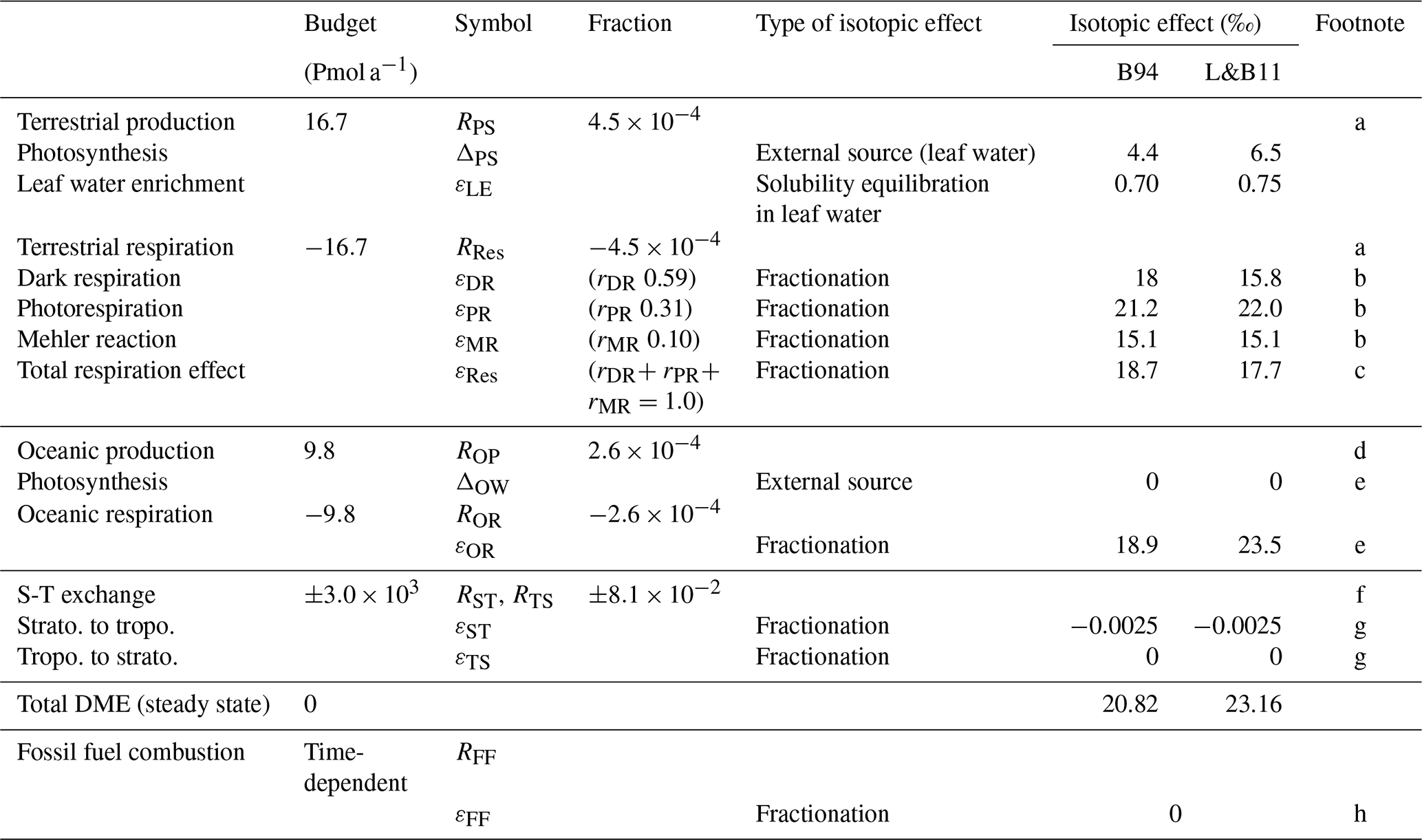
^a 16.7 Pmol a⁻¹ is the value by Hoffmann et al. (2004). R values were calculated by assuming that the total amount of atmospheric O₂ is 3.706×10⁴ Pmol. ^b The relative ratios of dark respiration, photorespiration, and Mehler reaction, as well as the isotopic effect of the Mehler reaction by B94. ^c $\mathrm{17.7}=\mathrm{0.59}\times \mathrm{15.8}+\mathrm{0.31}$ $\times \mathrm{22.0}+\mathrm{0.10}\times \mathrm{15.1}$, which becomes the same value by L&B11. ^d Calculated by using the ratio of 0.63:0.37 for the fraction of O₂ production by L&B11. ^e L&B11 showed that the total oceanic DME is 23.5 ‰ and that fractionations of oceanic photosynthesis exist. We assume that the same fractionation occurs only by respiration to realize the same extent of oceanic DME. ^f Calculated by using the net mass flux of S-T exchange in Olsen et al. (2004). ^g The stratospheric diminution effect was calculated as the ¹⁸O discrimination in stratosphere–troposphere exchange. Because the S-T exchange flux is about 100 times larger than the total terrestrial and oceanic flux, this contribution to the DME becomes about −0.3 ‰ ($-\mathrm{0.3}=R_{\mathrm{ST}}\times {\mathit{\epsilon }}_{\mathrm{ST}}$ $/$ (R_PS+R_OP)), which is the same value by L&B11. ^h We assume that atmospheric oxygen is consumed without isotope effects in fossil fuel combustion considering high temperature during industrial combustion processes.

Hoffmann et al. (2004) developed a model of the DME by combining the results of three-dimensional (3D) models of carbon and oxygen cycles with results of atmospheric general circulation models with built-in water isotope diagnostics and have obtained an average DME of 22.4 ‰ to 23.3 ‰. However, they did not simulate temporal or spatial variations of δ¹⁸O_atm in the present atmosphere, which have not yet been detected. The diurnal cycle of the atmospheric ${\mathrm{O}}_{\mathrm{2}}/{\mathrm{N}}_{\mathrm{2}}$ ratio at forest sites is caused mainly by activities in the terrestrial biosphere, and the peak-to-peak amplitudes are roughly 100 per meg (1 per meg is 0.001 ‰) (e.g., Ishidoya et al., 2013a; Battle et al., 2019; Faassen et al., 2023). Diurnal variations of δ¹⁸O_atm associated with activities in the terrestrial biosphere are therefore expected to be very small. Keeling (1995) predicted that δ_atm(¹⁸O) should be lower in summer than in winter in both hemispheres by about 2 per meg by assuming a 100 per meg seasonal increase in the atmospheric ${\mathrm{O}}_{\mathrm{2}}/{\mathrm{N}}_{\mathrm{2}}$ ratio due to the input of terrestrial and oceanic photosynthetic O₂, which has a δ(¹⁸O) that is lower than δ_atm(¹⁸O) by 20 ‰. Seibt et al. (2005), who calculated potential effects of human activity on the DME, estimated that global changes in the terrestrial biosphere may have led to a decrease in δ_atm(¹⁸O) on the order of 70 per meg over the last 150 years (−0.5 per meg a⁻¹). They have estimated that $\mathrm{2}/\mathrm{3}$ of the total decrease is due to a decrease in photorespiration globally accompanied by a 100 µmol mol⁻¹ increase in the fraction of atmospheric CO₂ during those 150 years. Diurnal, seasonal, and secular changes in δ_atm(¹⁸O) in the present atmosphere will therefore be a new indicator of activities of the land and oceanic biospheres, although sufficiently precise measurements of δ_atm(¹⁸O) to validate the suggestions by Keeling (1995) and Seibt et al. (2005) have never been reported.

In this study, we present diurnal, seasonal, and secular changes in δ_atm(¹⁸O) observed at Tsukuba (TKB), Japan (36° N, 140° E). We then compare the observed changes in δ_atm(¹⁸O) at TKB with a one-box model that incorporates the biosphere and water processes associated with the DME. To evaluate the secular changes in water processes, we used an isotope-enabled version of the Model for Interdisciplinary Research on Climate (MIROC5-iso) (Okazaki and Yoshimura, 2019) and calculated the δ(¹⁸O) of leaf water, δ_LW(¹⁸O). We suggest some applications of δ_atm(¹⁸O): (1) separation of the diurnal δ(${\mathrm{O}}_{\mathrm{2}}/{\mathrm{N}}_{\mathrm{2}}$) cycle into contributions from biological activities and fossil fuel combustion, (2) constraint of the seasonal δ_LW(¹⁸O) cycle, and (3) evaluation of recent secular changes in terrestrial gross primary production (GPP) and photorespiration.

2 Methods

2.1 Continuous atmospheric measurements of δ_atm(¹⁸O) and δ(${\mathrm{O}}_{\mathrm{2}}/{\mathrm{N}}_{\mathrm{2}}$)

Air was sampled with a diaphragm pump from an air intake located on the roof of a laboratory building of the National Institute of Advanced Industrial Science and Technology (AIST) at TKB. The gas velocity exceeded 5 m s⁻¹(4 mm i.d. and a flow rate of 4 L min⁻¹) at the tip of the air intake, which was high enough to prevent thermally diffusive inlet fractionation (Sturm et al., 2006; Blaine et al., 2006). The sample air was introduced into a 1 L, stainless-steel buffer tank after water vapor in the air had been reduced by using an electric cooling unit at 2 °C. The gas was then exhausted from the buffer tank at a flow rate of about 4 L min⁻¹. A small portion of this exhausted gas was introduced into a 3.2 mm (1/8 in.) o.d. stainless-steel tube, and any remaining water vapor was removed using a cold trap at −90 °C. Finally, the remaining sample air was vented through an outlet path at a rate of about 10 mL min⁻¹, and a minuscule amount of it was transferred to the ion source (or waste line) of a mass spectrometer (Thermo Fisher Scientific Delta V) through a thin, insulated, fused-silica capillary. The reference air was always supplied from a high-pressure cylinder at a flow rate of about 4 mL min⁻¹, and a minuscule amount of it was introduced into the ion source (or waste line) of the mass spectrometer through another fused-silica capillary. The standard air, which was supplied from a high-pressure cylinder at a flow rate of 4 mL min⁻¹, was introduced like the reference air into the ion source (or waste line) of the mass spectrometer, but through the line for sample air. We analyzed the standard air about once every 2 months. Details of the continuous measurement system we used have been reported by Ishidoya and Murayama (2014).

We repeatedly conducted alternate analyses of the sample and reference air for continuous measurements of stable isotopic ratios of O₂, N₂, and Ar (δ_atm(¹⁸O), δ_atm(¹⁵N), and δ_atm(⁴⁰Ar)) as well as the ${\mathrm{O}}_{\mathrm{2}}/{\mathrm{N}}_{\mathrm{2}}$ ratio and amount fraction of CO₂. The time required to obtain a measured value was 62 s. However, the standard deviation of the δ_atm(¹⁸O) was about 20 per meg, which was much larger than the standard deviation required to detect the expected respective seasonal (2 per meg) and secular changes (−0.5 per meg a⁻¹) in δ_atm(¹⁸O) calculated by Keeling (1995) and Seibt et al. (2005). We therefore averaged more than 1000 data points and used the averaged value as the observed δ_atm(¹⁸O). This averaging theoretically results in a standard error of the observed δ_atm(¹⁸O) of less than 0.6 per meg assuming no temporal drift during the averaging period. In this regard, we confirmed that the measured values of the δ_atm(¹⁸O) against reference air were stable enough for a period much longer than the averaging period. We therefore needed to calibrate with a primary and secondary air standard (described below) only once every 2 months. Figure 1 shows an example of the measured δ_atm(¹⁸O) of a standard air against reference air. We found the standard deviations of 200 and 400 averaged data points to be 1.4 and 0.4 per meg, respectively, which are consistent with the theoretically expected values of 1.3 and 1.0 per meg. In general, mass spectrometer behavior can change suddenly due to maintenance, such as a filament change or ion source tuning. To minimize the uncertainties associated with the changes in the conditions of the mass spectrometer, we used specific filaments for the measurements of air samples with the atmospheric level amount fraction of O₂ supplied by the Thermo Fisher Scientific. This enabled us to carry out continuous measurements in the present study for 11 months without exchanging the filament (when we used the original filament supplied for the mass spectrometer, then we needed to exchange it every 3 months). After the exchange of the filament, several weeks are needed to stabilize the condition of the ion source of the mass spectrometer by flowing the sample and reference air, especially for the elemental ratios of ${\mathrm{O}}_{\mathrm{2}}/{\mathrm{N}}_{\mathrm{2}}$, $\mathrm{Ar}/{\mathrm{N}}_{\mathrm{2}}$, and ${\mathrm{CO}}_{\mathrm{2}}/{\mathrm{N}}_{\mathrm{2}}$. Once the condition was stabilized, we did not tune the ion source throughout the period using the same filament. Furthermore, the mass spectrometer was dedicated only to measurements of δ_atm(¹⁸O) and related components, including those for flask samples (e.g., Ishidoya et al., 2021, 2022), and it was run day and night autonomously to keep the condition of the ion source.

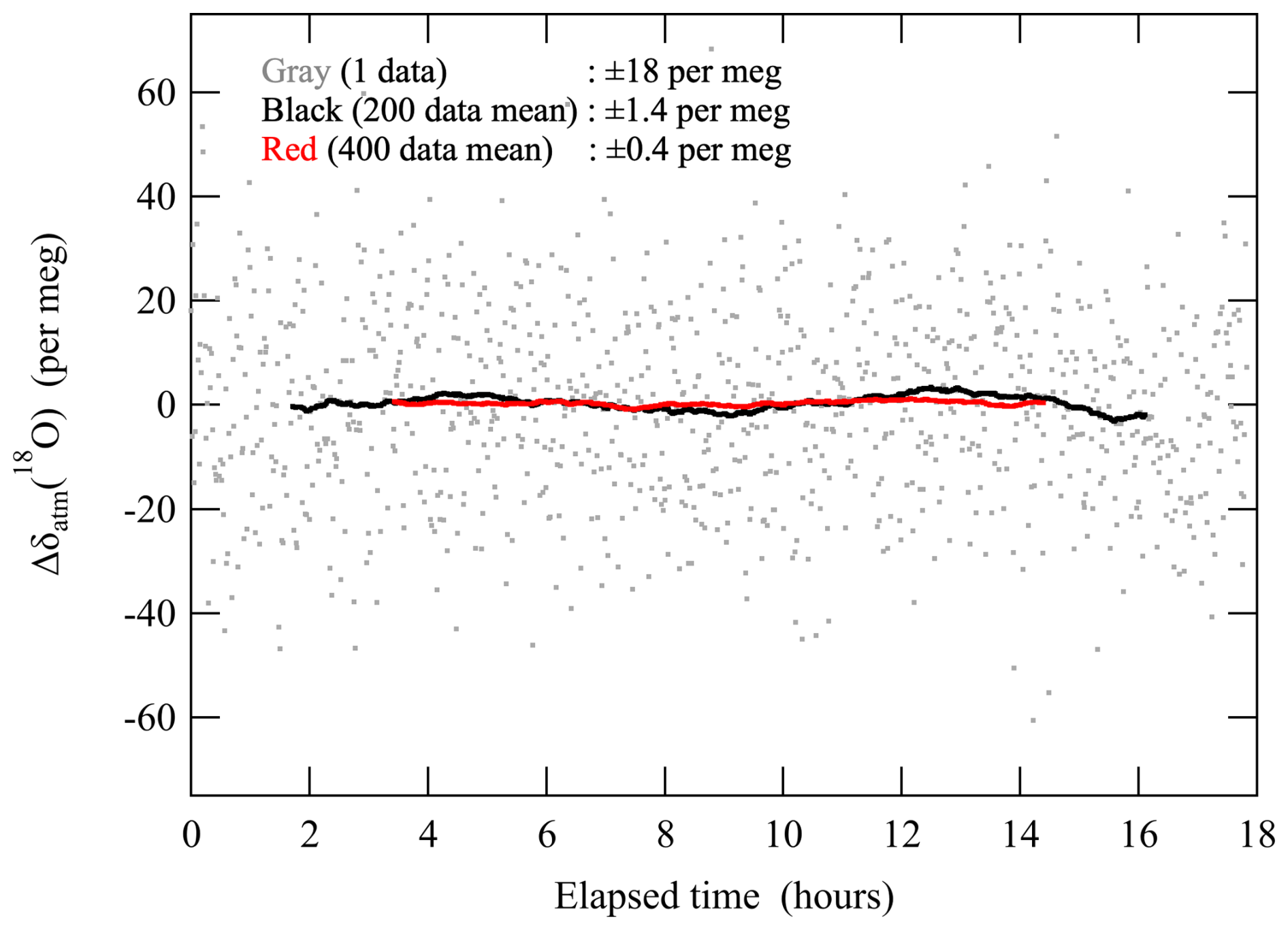
Figure 1 Typical analytical results of the difference (Δ) of the δ_atm(¹⁸O) of standard air against a reference air. Data are shown as deviations from the average value throughout the analysis. Gray dots, black lines, and red lines denote raw data and averages of 200 and 400 data points (corresponding to about 62 s, 3.5 h, and 7 h), respectively.

The δ_atm(¹⁸O) and δ(${\mathrm{O}}_{\mathrm{2}}/{\mathrm{N}}_{\mathrm{2}}$) are reported in per meg:

$$\begin{array}{}\text{(1)}& {\mathit{\delta }}_{\mathrm{atm}}\left({}^{\mathrm{18}}\mathrm{O}\right)={\displaystyle \frac{R_{\mathrm{sa}}\left({}^{\mathrm{18}}\mathrm{O}{}^{\mathrm{16}}\mathrm{O}/{}^{\mathrm{16}}\mathrm{O}{}^{\mathrm{16}}\mathrm{O}\right)-R_{\mathrm{st}}\left({}^{\mathrm{18}}\mathrm{O}{}^{\mathrm{16}}\mathrm{O}/{}^{\mathrm{16}}\mathrm{O}{}^{\mathrm{16}}\mathrm{O}\right)}{R_{\mathrm{st}}\left({}^{\mathrm{18}}\mathrm{O}{}^{\mathrm{16}}\mathrm{O}/{}^{\mathrm{16}}\mathrm{O}{}^{\mathrm{16}}\mathrm{O}\right)}},\end{array}$$

$$\begin{array}{}\text{(2)}& \mathit{\delta }\left({\mathrm{O}}_{\mathrm{2}}/{\mathrm{N}}_{\mathrm{2}}\right)={\displaystyle \frac{R_{\mathrm{sa}}\left({}^{\mathrm{16}}\mathrm{O}{}^{\mathrm{16}}\mathrm{O}/{}^{\mathrm{14}}\mathrm{N}{}^{\mathrm{14}}\mathrm{N}\right)-R_{\mathrm{st}}\left({}^{\mathrm{16}}\mathrm{O}{}^{\mathrm{16}}\mathrm{O}/{}^{\mathrm{14}}\mathrm{N}{}^{\mathrm{14}}\mathrm{N}\right)}{R_{\mathrm{st}}\left({}^{\mathrm{16}}\mathrm{O}{}^{\mathrm{16}}\mathrm{O}/{}^{\mathrm{14}}\mathrm{N}{}^{\mathrm{14}}\mathrm{N}\right)}}.\end{array}$$

Here, the subscripts “sa” and “st” indicate the sample air and the standard air, respectively. Because O₂ constitutes 0.2093 mol mol⁻¹ of air by volume (Aoki et al., 2019), a change of 4.8 per meg in δ(${\mathrm{O}}_{\mathrm{2}}/{\mathrm{N}}_{\mathrm{2}}$) is equivalent to about a change of 1 µmol mol⁻¹. In this study, the δ_atm(¹⁸O) and δ(${\mathrm{O}}_{\mathrm{2}}/{\mathrm{N}}_{\mathrm{2}}$) of each air sample were determined against our primary standard air (cylinder no. CRC00045) using a mass spectrometer. Our standards were dried in ambient air or industrially purified-air-based CO₂ in 48 L high-pressure aluminum cylinders. The standards were classified as either primary or secondary. Figure 2 shows the value of each analysis and the corresponding annual average of δ_atm(¹⁸O) of three secondary standards against the primary air standard. As shown in Fig. 2, variations of the annual average δ_atm(¹⁸O) of our three secondary standards were within ±0.8 to ±1.1 per meg (±0.9 per meg, on average) and nearly stable for 10 years with respect to the primary standard. We therefore allowed an uncertainty of ±0.9 per meg associated with the stability of the standard air for the annual average δ_atm(¹⁸O) in this study. This uncertainty corresponds to an uncertainty of ±0.13 ($\pm \sqrt{(\mathrm{0.9}{)}^{\mathrm{2}}+(\mathrm{0.9}{)}^{\mathrm{2}}}/\mathrm{10}$) per meg a⁻¹ for the 10-year-long secular trend.

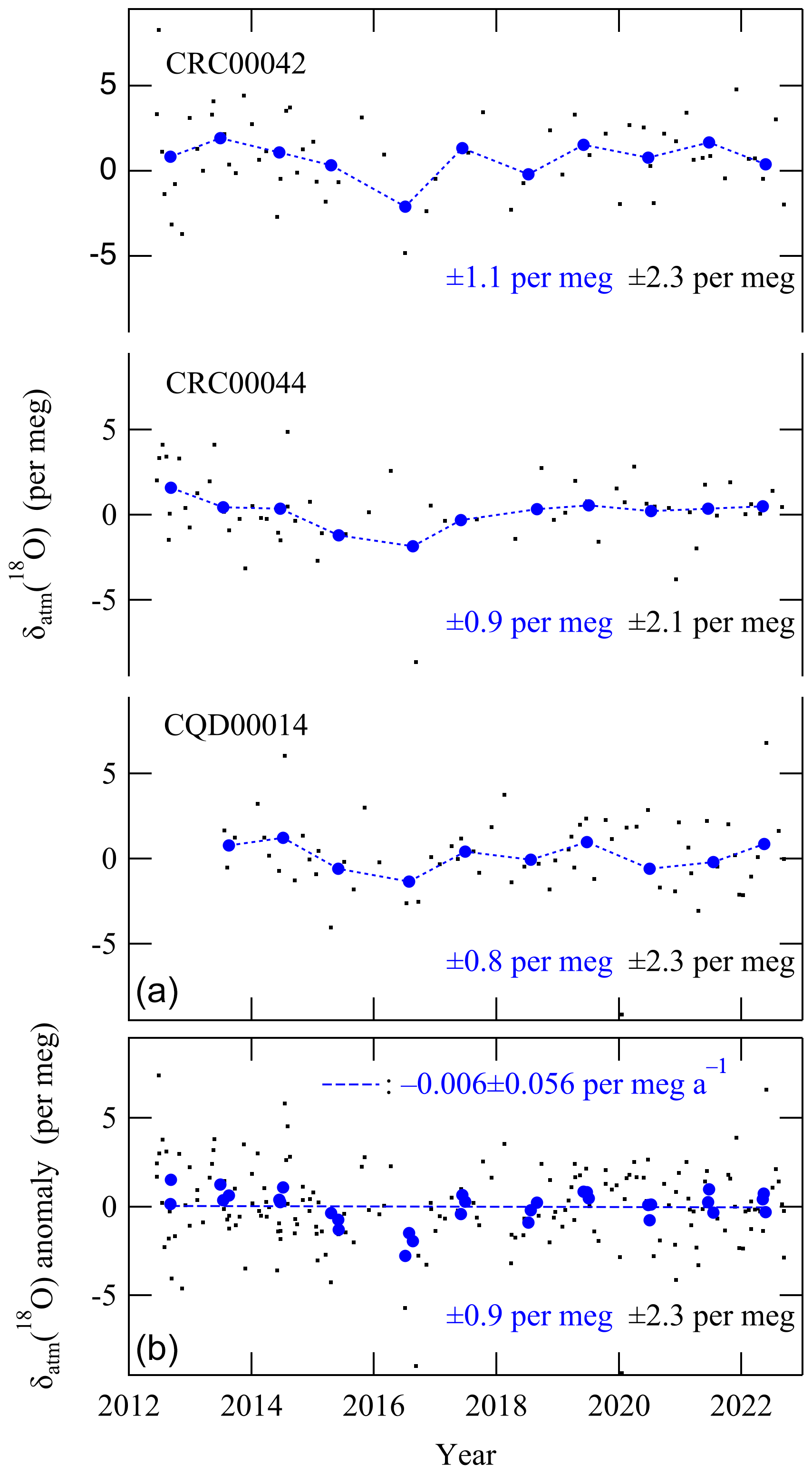
Figure 2 (a) Each value (black dots) and the corresponding annual average (blue circles) of δ_atm(¹⁸O) of three secondary standards against the primary standard air. (b) Anomalies of δ_atm(¹⁸O) of the three secondary standards. The dashed blue line denotes the regression line fit to the data.

We have examined the influence of the amount fraction of CO₂ in sample air on the δ(${\mathrm{O}}_{\mathrm{2}}/{\mathrm{N}}_{\mathrm{2}}$) measured on a mass spectrometer in past studies (Ishidoya et al., 2003; Ishidoya and Murayama, 2014). In this study, we also experimentally examined the influences of the amount fraction of CO₂ and the δ(${\mathrm{O}}_{\mathrm{2}}/{\mathrm{N}}_{\mathrm{2}}$) on δ_atm(¹⁸O). Figure 3a shows typical examples of the relationships between the measured δ_atm(¹⁸O) of the air sample and the amount fraction of CO₂. To obtain these relationships, a small amount of pure CO₂ was added to the flow line of the continuous measurement system during the analysis of standard air, or 1 L flasks were analyzed before and after a small amount of pure CO₂ was added to the flasks. The precision of the measurements of the flask air samples was about ±4 per meg. As seen in Fig. 3a, δ_atm(¹⁸O) increased linearly with increasing amount fractions of CO₂. We therefore decided to correct the δ_atm(¹⁸O) values by using amount fractions of CO₂ that were measured simultaneously. The mechanism of the positive correlation between δ_atm(¹⁸O) and CO₂ is not clarified yet since there is no isobaric interference. In this regard, we found no significant influences of CO₂ amount fraction on δ_atm(¹⁸O) for a different mass spectrometer: Finnigan MAT-252 (Ishidoya, 2003). This suggests that the influences should be examined carefully for each mass spectrometer. Figure 3b shows the relationships between the measured δ_atm(¹⁸O) values of the air samples and their δ(${\mathrm{O}}_{\mathrm{2}}/{\mathrm{N}}_{\mathrm{2}}$). To obtain these relationships, δ_atm(¹⁸O) and δ(${\mathrm{O}}_{\mathrm{2}}/{\mathrm{N}}_{\mathrm{2}}$) were measured for 1 L flasks or 48 L cylinders before and after pure N₂ was added to them. 1 L flasks were filled with the air in the cylinders for the analyses. It is apparent from Fig. 3b that we did not find a clearly increasing or decreasing trend of δ_atm(¹⁸O), at least when the δ(${\mathrm{O}}_{\mathrm{2}}/{\mathrm{N}}_{\mathrm{2}}$) was decreasing by about −8000 per meg. We therefore decided that we would not correct the δ_atm(¹⁸O) values for the changes in the simultaneously measured δ(${\mathrm{O}}_{\mathrm{2}}/{\mathrm{N}}_{\mathrm{2}}$). It is noteworthy that we obtained a different result – an increase in δ_atm(¹⁸O) with a decrease in δ(${\mathrm{O}}_{\mathrm{2}}/{\mathrm{N}}_{\mathrm{2}}$) – in our earlier flask studies in 2013. We have not yet clarified the cause(s), but we expect the results shown in Fig. 3b to be valid because we repeatedly obtained results that were consistent between flasks and cylinders.

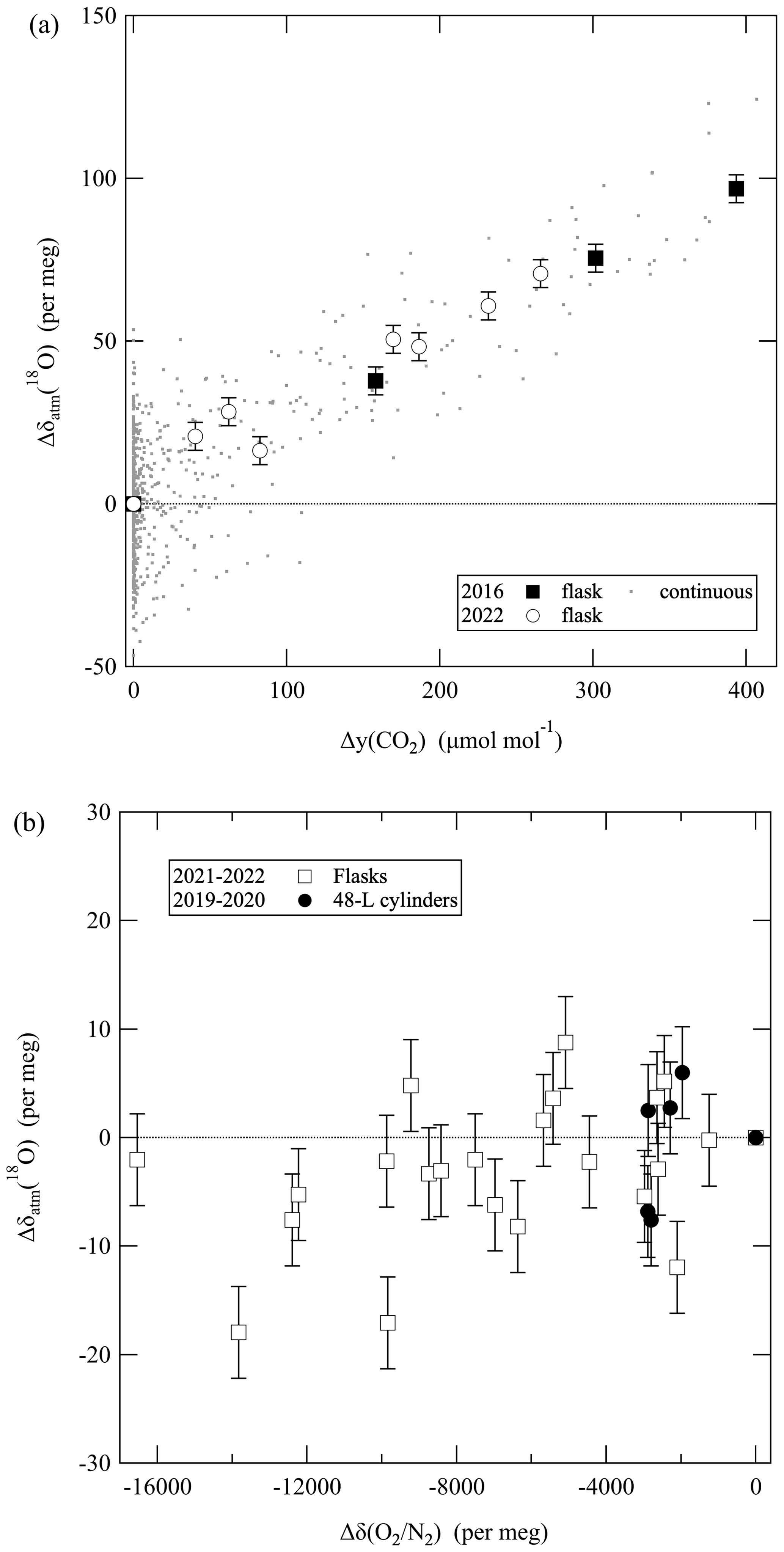
Figure 3 (a) Changes (Δ) in the measured δ_atm(¹⁸O) of air samples as a function of the amount fraction of CO₂. Δy(CO₂) represents the difference between the amount fraction of CO₂ of the air sample after and before adding pure CO₂. y stands for the dry amount fraction of gas. (b) Changes in the measured δ_atm(¹⁸O) of the air sample as a function of its δ(${\mathrm{O}}_{\mathrm{2}}/{\mathrm{N}}_{\mathrm{2}}$). Δδ(${\mathrm{O}}_{\mathrm{2}}/{\mathrm{N}}_{\mathrm{2}}$) represents the difference between the δ(${\mathrm{O}}_{\mathrm{2}}/{\mathrm{N}}_{\mathrm{2}}$) of the air sample after and before adding pure N₂. Error bars in (a) and (b) indicate uncertainties (±1σ) for the measurements of air samples in flasks.

2.2 Box model for simultaneous analysis of δ_atm(¹⁸O) and δ(${\mathrm{O}}_{\mathrm{2}}/{\mathrm{N}}_{\mathrm{2}}$)

The box model used in this study is the same as that described by B94. However, the isotopic effects for the sink–source processes are updated by a more recent study of L&B11. Therefore, we performed calculations using the isotope effects from both studies and compared them, especially for the long-term variations of δ_atm(¹⁸O). Since there are a lot of symbols used in this study, we present a list of the symbols in the main text in Table A1 in Appendix A. Equation (3) is the mass balance equation for δ_atm(¹⁸O) (see Appendix B for derivation).

$$\begin{array}{}\text{(3)}& \begin{array}{rl}{\displaystyle \frac{\mathrm{d}{\mathit{\delta }}_{\mathrm{atm}}\left({}^{\mathrm{18}}\mathrm{O}\right)}{\mathrm{d}t}}& =\left({\mathit{\epsilon }}_{\mathrm{MR}}{r}_{\mathrm{MR}}+{\mathit{\epsilon }}_{\mathrm{PR}}{r}_{\mathrm{PR}}+{\mathit{\epsilon }}_{\mathrm{DR}}{r}_{\mathrm{DR}}\right)R_{\mathrm{Res}}\\ & +\left({\mathrm{\Delta }}_{\mathrm{PS}}-{\mathit{\epsilon }}_{\mathrm{LE}}-{\mathit{\delta }}_{\mathrm{atm}}\right)R_{\mathrm{PS}}+{\mathit{\epsilon }}_{\mathrm{OR}}{R}_{\mathrm{OR}}\\ & +\left({\mathrm{\Delta }}_{\mathrm{OW}}-{\mathit{\delta }}_{\mathrm{atm}}\right)R_{\mathrm{OP}}+{\mathit{\epsilon }}_{\mathrm{TS}}{R}_{\mathrm{TS}}+{\mathit{\epsilon }}_{\mathrm{ST}}{R}_{\mathrm{ST}}\\ & +{\mathit{\epsilon }}_{\mathrm{FF}}{R}_{\mathrm{FF}},\end{array}\end{array}$$

where r_MR, r_PR, and r_DR are the relative ratios of the Mehler reaction, photorespiration, and dark respiration to the total O₂ consumption associated with terrestrial respiration, and ε_MR, ε_PR, ε_DR, ε_LE, and ε_OR denote the isotope effects of the Mehler reaction, photorespiration, dark respiration, leaf water enrichment, and marine respiration, respectively. Values of O₂ budgets and isotopic effects are summarized in Table 1. The isotopic enrichment of O₂ produced by the terrestrial photosynthesis, Δ_PS, is basically determined by the δ_LW(¹⁸O)(Gonfiantini et al., 1965; Dongmann et al., 1972; Farquhar et al., 1993), and we assumed Δ_PS to be 4.4 ‰ or 6.5 ‰ for the steady state. There is still a large uncertainty in δ_LW(¹⁸O)(Farquhar et al., 1993; Bender et al., 1994; Hoffmann et al., 2004; Keeling 1995; West et al., 2008). In this study, we used the δ_LW(¹⁸O) calculated by a 3D model (see Sect. 3.2 and 3.3). We used values of the relative ratios for the respiration (r_MR, r_PR, and r_DR) following B94. Specifically, respective values of r_MR, r_PR, and r_DR are 0.1, 0.31, and 0.59 in B94. As a result, the total isotope effects of terrestrial respiration become 18.7 ‰ and 17.7 ‰ for B94 and L&B11, respectively. This difference is caused by the large difference of their dark respiration effects (ε_DR). The biggest difference between the two studies is the effect of the ocean, and the respective oceanic DMEs are 18.9 ‰ and 23.5 ‰ for B94 and L&B11. The oceanic DME for L&B11 is almost the same magnitude as the total terrestrial DMEs, which are 22.4 (4.4–0.70 + 18.7) ‰ and 23.5 (6.5–0.75 + 17.7) ‰ for B94 and L&B11, respectively. L&B11 also showed that photosynthetic enrichment in the ocean cannot be ignored, contrary to previous studies. However, they did not clearly separate the effects of oceanic photosynthesis and respiration. Therefore, we assumed Δ_OW and ε_OR to be zero and 23.5 ‰, respectively, to set the total oceanic DME to be 23.5 ‰ as L&B11. Unlike the previous studies, the stratospheric effect was formulated as fractionations, ε_TS and ε_ST, which denote the isotope effects of air exchange between the troposphere and stratosphere. This is because we have continued precise measurements of the isotopic ratios of O₂ in the stratosphere, which could provide new insights into stratospheric processes, as described later. R_Res, R_PS, R_OR, and R_OP (the unit is a⁻¹) represent the relative ratios of the annual fluxes of O₂ from terrestrial respiration, terrestrial production, marine respiration, and marine production, respectively, to the total amount of O₂ in the atmosphere ($=\mathrm{3.706}\times {\mathrm{10}}^{\mathrm{4}}$ Pmol). For example, if we assume that the terrestrial flux is 16.7 Pmol a⁻¹, R_PS will be 16.7/(3.706 × 10⁴) = 4.5× 10⁻⁴ a⁻¹, as shown in Table 1. R_TS and R_ST denote the relative ratios of the annual fluxes of O₂ between the troposphere and stratosphere, respectively. ε_FF and R_FF denote the isotopic effects in fossil fuel combustion and the relative ratios of the annual O₂ consumption by fossil fuel combustion, respectively. We assumed that atmospheric oxygen is consumed without isotope effects in fossil fuel combustion (ε_FF=0), taking into account that industrial combustion processes usually occur at high temperature. Therefore, we consider no contribution to DME from fossil fuel combustion in this study. In this regard, it is known that large oxygen isotope fractionation occurs in combustion processes such as biomass burning due to complex combustion processes (Schumacher et al., 2011). In such cases, it will be necessary to consider isotopic fractionation in the consumption of atmospheric oxygen associated with combustion. However, at present, little is known about the impact of this on DME. The box model also calculates the amount fraction of atmospheric O₂, y(O₂) by solving the following mass balance equation:

$$\begin{array}{}\text{(4)}& \begin{array}{rl}{\displaystyle \frac{\mathrm{1}}{y\left({\mathrm{O}}_{\mathrm{2}}\right)}}& {\displaystyle \frac{\mathrm{d}y\left({\mathrm{O}}_{\mathrm{2}}\right)}{\mathrm{d}t}}=\left(r_{\mathrm{MR}}+r_{\mathrm{PR}}+r_{\mathrm{DR}}\right)R_{\mathrm{Res}}+R_{\mathrm{PS}}+R_{\mathrm{OR}}\\ & +R_{\mathrm{OP}}+R_{\mathrm{TS}}+R_{\mathrm{ST}}+R_{\mathrm{FF}}.\end{array}\end{array}$$

Here, y stands for the dry amount fraction of gas, as recommended by the IUPAC Green Book (Cohen et al., 2007). To compare with the observed results for δ(${\mathrm{O}}_{\mathrm{2}}/{\mathrm{N}}_{\mathrm{2}}$), the amount fraction of O₂ calculated by the box model was converted to δ(${\mathrm{O}}_{\mathrm{2}}/{\mathrm{N}}_{\mathrm{2}}$) assuming a normal atmosphere.

We assumed the value of terrestrial O₂ production, P_T, to be 16.7 Pmol a⁻¹, which is the value reported by Hoffmann et al. (2004). The ratio of terrestrial and marine production was assumed to be 0.63:0.37 (Luz and Barkan, 2011). It is known that mass-independent isotopic fractionation of ¹⁷O and ¹⁸O between O₃ and CO₂ occurs in the stratosphere via photochemical processes (e.g., Gamo et al., 1989; Thiemens, 1999). B94 estimated the isotopic effect on atmospheric O₂ by scaling the δ(¹⁸O) of CO₂ and calculated that it would reduce δ_atm(¹⁸O) by 0.4 ‰, considering the turnover time between the troposphere and the stratosphere. L&B11 showed that the global Δ(¹⁷O) budget supports their result and have estimated the stratospheric isotope effect on δ_atm(¹⁸O) to be 0.3 ‰. In this study, the flux between the troposphere and stratosphere was set to 3000 Pmol a⁻¹, which is calculated from the stratosphere–troposphere (S-T) mass flux (Olsen et al., 2004). This S-T O₂ flux is approximately 100 times the flux from the biosphere (Luz et al., 1999). ε_ST, which is the isotopic fractionation of O₂ that returns from the stratosphere to the troposphere, is currently considered to be so small that it is impossible to actually detect it in the stratosphere. Note that ε_ST represents the fractionation of stratosphere–troposphere exchange flux in this study, while ε_strat in L&B11 represents the stratospheric effect on DME. As a rough estimate, considering that the value of Δ(¹⁷O) is −1.5 per meg with respect to the tropospheric value (Luz et al., 1999), ε_ST is expected to be about −3 per meg based on the mass-independent effect (δ¹⁷O ≈δ¹⁸O). Here, ε_ST was set to −2.5 per meg so that the diminution of δ_atm(¹⁸O) at equilibrium was −0.3 ‰. Because there are no isotopic effects during the transport of air from the troposphere to the stratosphere, ε_TS should be zero.

Based on the above discussion, the δ(¹⁸O) in the stratosphere should be −2.5 to −3 per meg lower than in the troposphere due to photochemical processes. As a matter of fact, the δ(¹⁸O) of stratospheric O₂ has been observed with high precision by balloon experiments and is known to decrease significantly with increasing altitude because of gravitational separation (e.g., Ishidoya et al., 2013b; Sugawara et al., 2018). At an altitude of 35 km over Japan, δ(¹⁸O) is lower than the tropospheric value by approximately −100 per meg, which is anomalously lower (i.e., larger diminution) than that expected on the basis of photochemical diminution. The implication is that enrichment of approximately 5 per meg is permanently occurring in the troposphere because of gravitational separation in the stratosphere (Ishidoya et al., 2021). It is currently uncertain how gravitational separation affects the process by which isotopically light oxygen is transported to the troposphere through troposphere–stratosphere exchange. For example, changing ε_ST from −2.5 to −5.0 per meg yields the δ_atm(¹⁸O) trend of approximately −0.2 per meg a⁻¹ because the flux from the stratosphere is over 100 times greater than the surface biospheric flux. This uncertainty complicates the problem of interannual δ_atm(¹⁸O) change and suggests that gravitational separation may be involved in small fluctuations in the DME.

With these initial settings, we were able to reach a steady state after a 5000-year simulation, and we found that the equilibrium values of δ_atm(¹⁸O) were 20.82 ‰ and 23.16 ‰ for calculations following B94 and L&B11, respectively, which are almost same values reported by the two studies. Hereafter, the box model results are discussed based on the differences from these equilibrium values. The biospheric turnover time of O₂ in the steady state was 1398 years, which is longer than the 1200 years estimated by B94. This may be a little too long, since the δ_atm(¹⁸O) variations reported by Severinghaus et al. (2009) based on ice core measurements showed a characteristic asymptotic decay curve after abrupt climate change events on a timescale of about ∼ 1000 years, implying that the turnover time of O₂ in the atmosphere is about 1000 years. The biospheric turnover time is inversely proportional to the sum of the terrestrial and oceanic production of O₂ incorporated into the box model, which is 26.5 (16.7 + 9.8) Pmol a⁻¹ in this study (Table 1). This implies that total production of O₂ for the initial value in our model is underestimated. In this regard, turnover time decreases to about 1000 years when we simulate a case in which the GPP is increased, as will be discussed later. In model calculations for the interpretation of long-term changes, we used the steady-state condition described above as the initial condition, and we performed some calculations by adding long-term changes to terrestrial GPP, photorespiration, and δ_LW(¹⁸O)(see details in Sect. 3.3).

The box model was suitable for simulations if we assumed that long-term and global changes occurred over time frames of hundreds to thousands of years. The box model naturally ignores atmospheric transport processes, and it is difficult to define the box atmosphere at local and regional spatial scales. There is hence a theoretical limit to the application of the box model to short-timescale phenomena. However, we tried to use this box model as a first step to understand the diurnal and seasonal changes in δ_atm(¹⁸O) recently observed by high-precision measurements. Because δ(${\mathrm{O}}_{\mathrm{2}}/{\mathrm{N}}_{\mathrm{2}}$) was also observed at the same time during this study, the relationships between δ_atm(¹⁸O) and δ(${\mathrm{O}}_{\mathrm{2}}/{\mathrm{N}}_{\mathrm{2}}$) provided information about the usefulness of the box model simulations. For the simulations of diurnal changes, the intensities of terrestrial O₂ consumption and production were approximated by a simple function, which became a maximum at noon and zero during the night. We also carried out simulations of diurnal changes considering marine O₂ consumption and production approximated by the similar simple function to examine sensitivities of the ${\mathit{\delta }}_{\mathrm{atm}}{(}^{\mathrm{18}}\mathrm{O})/\mathit{\delta }$(${\mathrm{O}}_{\mathrm{2}}/{\mathrm{N}}_{\mathrm{2}}$) ratio to the terrestrial and marine signals. Seasonal variations were also simulated by a simple sinusoidal function. We then tuned the magnitude of R_Res (=R_PS) so that the amplitude of the modeled δ(${\mathrm{O}}_{\mathrm{2}}/{\mathrm{N}}_{\mathrm{2}}$) variation was close to the observed results. The box model did not incorporate the contributions of S-T O₂ flux and fossil fuel combustion for the simulations of the diurnal and seasonal changes.

2.3 Numerical simulations of δ_LW(¹⁸O) using the 3D model MIROC5-iso

We simulated δ_LW(¹⁸O) using a stable-water-isotope-enabled general circulation model named MIROC5-iso (Okazaki and Yoshimura, 2017, 2019). MIROC5-iso is the fifth generation of the Model for Interdisciplinary Research on Climate (MIROC5; Watanabe et al., 2010). The stable water isotopes were implemented to the atmospheric and land surface components following Jouzel et al. (1987) and Yoshimura et al. (2006). MIROC5-iso calculates the isotopic ratio of atmospheric water vapor, precipitation, and reservoirs at ground level, including soil water and leaf water, with the equilibrium and kinetic fractionation at all phase transitions. The δ_LW(¹⁸O) is calculated by considering water conveyance driven by transpiration and diffusive isotopic movement (i.e., “back diffusion”) as follows:

$$\begin{array}{}\text{(5)}& {\displaystyle \frac{\mathrm{d}{V}_{\mathrm{L}}}{\mathrm{d}{z}_{\mathrm{L}}}}{\displaystyle \frac{\partial R_{\mathrm{LW}}}{\partial t}}={\displaystyle \frac{\mathrm{1}}{\mathit{\rho }}}\left({\displaystyle \frac{T{A}_{\mathrm{L}}}{I_{\mathrm{LA}}}}{\displaystyle \frac{\partial R_{\mathrm{LW}}}{\partial z_{\mathrm{L}}}}-D\mathit{\tau }{\displaystyle \frac{{\partial }^{\mathrm{2}}{R}_{\mathrm{LW}}}{\partial z_{\mathrm{L}}^{\mathrm{2}}}}\right).\end{array}$$

Here, R_LW is the isotopic ratio of the leaf water given by $R_{\mathrm{LW}}=R_{\mathrm{sample}}\left({\mathrm{H}}_{\mathrm{2}}^{\mathrm{18}}\mathrm{O}/{\mathrm{H}}_{\mathrm{2}}^{\mathrm{16}}\mathrm{O}\right)/R_{\mathrm{standard}}$ $\left({\mathrm{H}}_{\mathrm{2}}^{\mathrm{18}}\mathrm{O}/{\mathrm{H}}_{\mathrm{2}}^{\mathrm{16}}\mathrm{O}\right)$, where the subscripts “sample” and “standard” indicate the sample and the standard water, respectively, and the standard water is VSMOW. z_L is the axis directed from the leaf base to tip, and V_L and A_L are the volume of leaf water and area of the leaf surface, respectively. ρ is the density of water, T is the transpiration flux, I_LA is the leaf area index, D is the liquid diffusivity of an isotope, and τ is the crookedness of the leaf. The transpired water drawn up from the root zone layers is calculated by weighting the isotope ratio of soil water by root density. The transpiration fluxes of the water isotopes were calculated by the bulk method with the bulk exchange coefficient of Sellers et al. (1996), and the equilibrium and kinetic fractionations from liquid to gas at the stoma were considered.

In this study, MIROC5-iso was forced by observed sea surface temperature, sea ice concentration, observed greenhouse gases (carbon dioxide, methane, and chlorofluorocarbons), ozone, and changes in land use. The isotopic compositions of sea surface water and sea ice were kept constant and assumed to be 0 ‰ and 3 ‰ , respectively, as in Joussaume and Jouzel (1993). The model resolution was set to T42 (approximately 280 km at the Equator) with 40 vertical levels. After running MIROC5-iso for 100 years with the condition of 1871 CE for spin-up, we ran the model from 1871–2022 CE.

3 Results and discussion

3.1 Diurnal variations of δ_atm(¹⁸O) and δ(${\mathrm{O}}_{\mathrm{2}}/{\mathrm{N}}_{\mathrm{2}}$)

Figure 4a shows the average diurnal cycles of δ_atm(¹⁸O), δ(${\mathrm{O}}_{\mathrm{2}}/{\mathrm{N}}_{\mathrm{2}}$), the amount fraction of CO₂, and δ($\mathrm{Ar}/{\mathrm{N}}_{\mathrm{2}}$) for each season observed at TKB during 2013–2022. δ($\mathrm{Ar}/{\mathrm{N}}_{\mathrm{2}}$) was defined in the same way as δ(${\mathrm{O}}_{\mathrm{2}}/{\mathrm{N}}_{\mathrm{2}}$) but for the ${}^{\mathrm{40}}\mathrm{Ar}{/}^{\mathrm{14}}{\mathrm{N}}^{\mathrm{14}}\mathrm{N}$ ratio. The error bands shown in Fig. 4a indicate year-to-year variations of the average diurnal cycles (± 1σ). In this study, we needed to remove any natural or artificial fractionation of ¹⁸O¹⁶O and ¹⁶O¹⁶O, other than the processes associated with the DME from the observed δ_atm(¹⁸O). For this purpose, we used the observed diurnal δ($\mathrm{Ar}/{\mathrm{N}}_{\mathrm{2}}$) cycle, which is potentially driven by the nighttime vertical temperature gradient (Adachi et al., 2006) and artificial inlet fractionation induced by radiative heating of an air intake (e.g., Blaine et al., 2006). The δ($\mathrm{Ar}/{\mathrm{N}}_{\mathrm{2}}$) underwent a slight diurnal cycle with a maximum in the early morning (Fig. 4a), and the difference between the maximum and minimum was about 4–6 per meg. It is difficult to specify the cause of the diurnal cycle, but it may result from natural variations due to a nighttime vertical temperature gradient at the inland TKB site because Adachi et al. (2006) reported much larger enrichment of δ($\mathrm{Ar}/{\mathrm{N}}_{\mathrm{2}}$) by 100 per meg at the center of a wide desert during the night. We therefore decided to correct the observed values for thermally diffusive fractionation following the method used by Ishidoya et al. (2014, 2022) and to use the corrected values for our discussion of diurnal variations. Specifically, we subtracted $\left(\mathrm{1.55}/\mathrm{16.2}\right)\times \mathit{\delta }(\mathrm{Ar}/{\mathrm{N}}_{\mathrm{2}})$ from the observed δ_atm(¹⁸O). The coefficient 1.55$/$16.2 is the ${\mathit{\delta }}_{\mathrm{atm}}{(}^{\mathrm{18}}\mathrm{O})/\mathit{\delta }$($\mathrm{Ar}/{\mathrm{N}}_{\mathrm{2}}$) ratio determined by laboratory experiments (Ishidoya et al., 2013b). In a similar manner, we also corrected the δ(${\mathrm{O}}_{\mathrm{2}}/{\mathrm{N}}_{\mathrm{2}}$) for thermally diffusive fractionation by subtracting $\left(\mathrm{4.57}/\mathrm{16.2}\right)\times \mathit{\delta }(\mathrm{Ar}/{\mathrm{N}}_{\mathrm{2}})$ from the measured δ(${\mathrm{O}}_{\mathrm{2}}/{\mathrm{N}}_{\mathrm{2}}$). The coefficient 4.57/16.2 is the $\mathit{\delta }\left({\mathrm{O}}_{\mathrm{2}}/{\mathrm{N}}_{\mathrm{2}}\right)/\mathit{\delta }$($\mathrm{Ar}/{\mathrm{N}}_{\mathrm{2}}$) ratio from the same laboratory experiments. The maximum corrections were 0.3 and 1.0 per meg for δ_atm(¹⁸O) and δ(${\mathrm{O}}_{\mathrm{2}}/{\mathrm{N}}_{\mathrm{2}}$), respectively. The correction for the amount fraction of CO₂ was negligibly small.

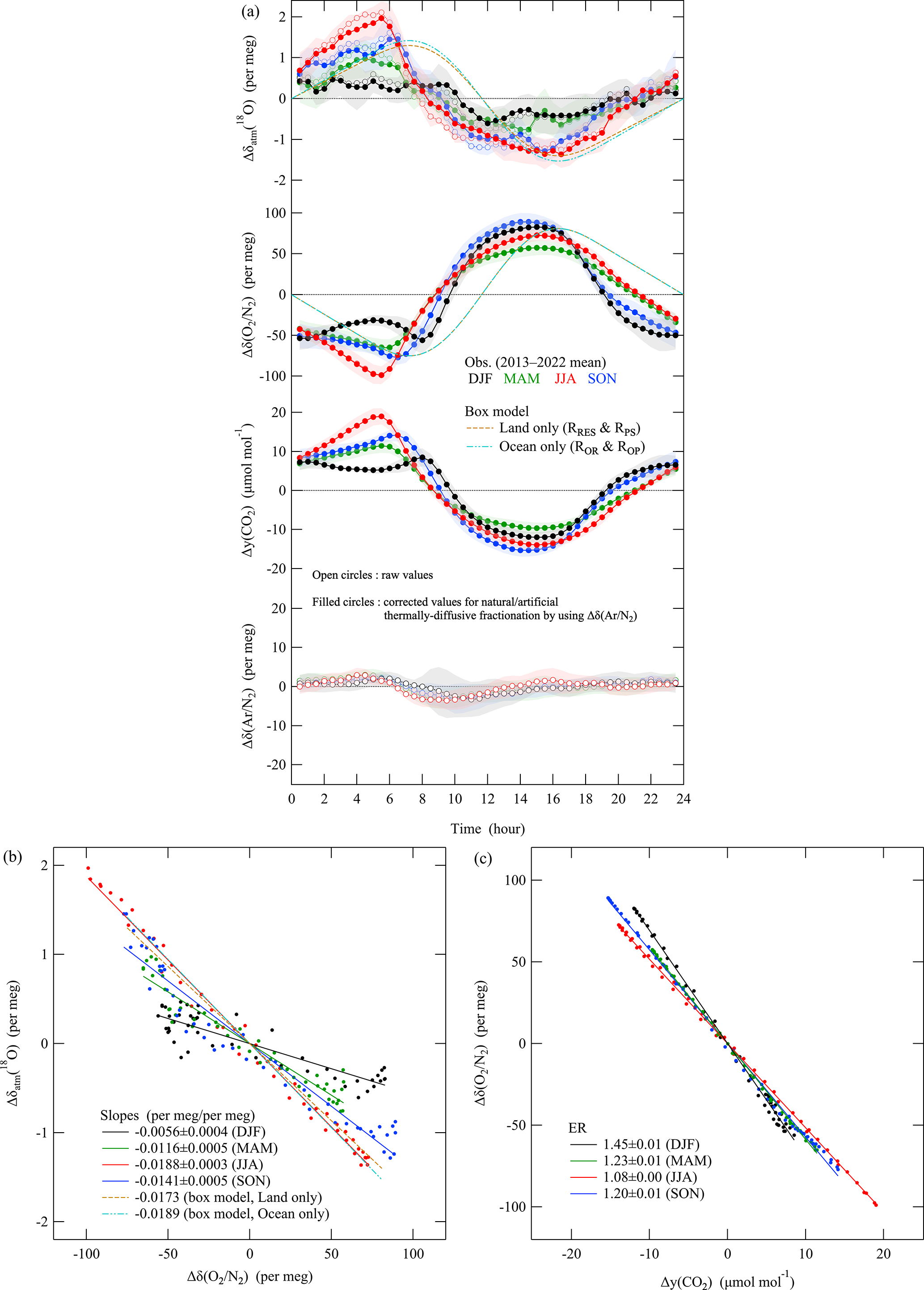
Figure 4 (a) Plots of the average diurnal cycles of Δδ_atm(¹⁸O), Δδ(${\mathrm{O}}_{\mathrm{2}}/{\mathrm{N}}_{\mathrm{2}}$), Δy(CO₂), and Δδ(Ar/N₂) (open circles) observed at the TKB site during 2013–2022 for each season: December to February (black), March to May (green), June to August (red), and September to November (blue). Error bands indicate year-to-year variations during the observation periods (±1σ). Those of Δδ_atm(¹⁸O), Δδ(${\mathrm{O}}_{\mathrm{2}}/{\mathrm{N}}_{\mathrm{2}}$), and Δy(CO₂), corrected for thermally diffusive fractionation, are also plotted (filled circles) (see text). The range of the vertical axis for Δδ($\mathrm{Ar}/{\mathrm{N}}_{\mathrm{2}}$) was adjusted arbitrarily to facilitate visual assessment of the variations of the observed Δδ_atm(¹⁸O) due to thermally diffusive fractionation. Average diurnal cycles of Δδ_atm(¹⁸O) and Δδ(${\mathrm{O}}_{\mathrm{2}}/{\mathrm{N}}_{\mathrm{2}}$) that were simulated with a box model are also shown. The simulated values that considered only terrestrial and marine respiration and production are shown by the dashed ocher line and the dashed light blue two-dotted line, respectively (see text). Δ denotes deviations from the diurnal mean values. (b) Relationships between Δδ_atm(¹⁸O) and Δδ(${\mathrm{O}}_{\mathrm{2}}/{\mathrm{N}}_{\mathrm{2}}$) for the data corrected for thermally diffusive fractionation in (a). Regression lines fitted to the observed and simulated data are also shown. (c) Same as in (b) but for the relationship between Δδ(${\mathrm{O}}_{\mathrm{2}}/{\mathrm{N}}_{\mathrm{2}}$) and Δy(CO₂).

δ_atm(¹⁸O) exhibited a clear diurnal cycle with a daytime minimum, especially in summer (Fig. 4a). δ_atm(¹⁸O) varied out of phase with δ(${\mathrm{O}}_{\mathrm{2}}/{\mathrm{N}}_{\mathrm{2}}$), and the ratio of the amplitude of the diurnal δ_atm(¹⁸O) cycles to those of δ(${\mathrm{O}}_{\mathrm{2}}/{\mathrm{N}}_{\mathrm{2}}$) was substantially larger in summer than in winter. Figure 4a also shows the diurnal cycles of δ_atm(¹⁸O) and δ(${\mathrm{O}}_{\mathrm{2}}/{\mathrm{N}}_{\mathrm{2}}$) simulated by the box model described in Sect. 2.2 that incorporated the isotopic effects from B94. The simulations were carried out under two conditions: one was the case when we ignored marine respiration and the production of O₂ (R_OR and R_OP), and the other was the case when we ignored terrestrial respiration and the production of O₂ (R_Res and R_PS). In both cases, the R_Res and R_PS (or R_OR and R_OP) in the model were adjusted to reproduce the observed seasonal δ (${\mathrm{O}}_{\mathrm{2}}/{\mathrm{N}}_{\mathrm{2}}$) cycle subject to the constraint that the daily average R_Res=R_PS (or R_OR=R_OP). The initial value of the δ_atm(¹⁸O) relative to ocean water was then adjusted arbitrarily to establish a steady state for the simulated δ_atm(¹⁸O). The δ(¹⁸O) values relative to ocean water in the steady state were 22.0 ‰ and 18.9 ‰ for the case when we considered only terrestrial or only marine respiration and production, respectively. We found that the general characteristics of the diurnal cycles of δ_atm(¹⁸O) and δ(${\mathrm{O}}_{\mathrm{2}}/{\mathrm{N}}_{\mathrm{2}}$) were reproduced by the simulated δ_atm(¹⁸O) for both cases when we considered only terrestrial or only marine processes (Fig. 4a).

To determine the cause(s) of the observed diurnal δ_atm(¹⁸O) cycles, we examined the relationships between the observed δ_atm(¹⁸O) and δ(${\mathrm{O}}_{\mathrm{2}}/{\mathrm{N}}_{\mathrm{2}}$) (Fig. 4b) and those for δ(${\mathrm{O}}_{\mathrm{2}}/{\mathrm{N}}_{\mathrm{2}}$) and the amount fraction of CO₂ (Fig. 4c). The ${\mathit{\delta }}_{\mathrm{atm}}{(}^{\mathrm{18}}\mathrm{O})/\mathit{\delta }$(${\mathrm{O}}_{\mathrm{2}}/{\mathrm{N}}_{\mathrm{2}}$) ratios were −0.019 and −0.006 per meg (per meg)⁻¹ in summer and winter, respectively. In Fig. 4b, we also plot the relationship between the simulated δ_atm(¹⁸O) and δ(${\mathrm{O}}_{\mathrm{2}}/{\mathrm{N}}_{\mathrm{2}}$). We found the simulated ratios to be –0.017 and −0.019 per meg (per meg)⁻¹ when we considered only terrestrial or only marine respiration and production, respectively. These ratios were much closer to the ratio observed in summer than in winter. The O₂ and CO₂ exchange ratios (ERs, −Δy(O₂)Δy(CO₂)⁻¹) calculated from the δ(${\mathrm{O}}_{\mathrm{2}}/{\mathrm{N}}_{\mathrm{2}}$) and the amount fraction of CO₂ shown in Fig. 4c were 1.08 and 1.45 in summer and winter, respectively. An oxidative ratio (OR, −Δy(O₂)Δy(CO₂)⁻¹) of 1.05–1.1 is expected for terrestrial biosphere activities, and ratios of 1.17, 1.44, and 1.95 are expected for combustion of solid fuel, liquid fuel, and natural gas, respectively (Keeling, 1988; Severinghaus, 1995). The ER refers to the exchange between the atmosphere and organisms or ecosystems, whereas the OR reflects the stoichiometry of specific materials, in accord with Faassen et al. (2023) and Ishidoya et al. (2024). The ORs therefore suggested that the diurnal δ(${\mathrm{O}}_{\mathrm{2}}/{\mathrm{N}}_{\mathrm{2}}$) cycle observed in summer could be attributed mainly to terrestrial biosphere activities, whereas that in winter was due to fossil fuel combustion. The observed wintertime ER of 1.45 was also consistent with the average OR of 1.52 ± 0.1 for fossil fuel consumption (hereafter referred to as OR_FF) for the Kanto area, which includes TKB, of about 1.7×10⁴ km², calculated using the data on fossil fuel consumption reported by the Agency of Natural Resources and Energy (https://www.enecho.meti.go.jp/statistics/energy_consumption/ec002/results.html#headline2, last access: 28 March 2024, in Japanese) (Ishidoya et al., 2020). The implication is therefore that the isotopic discrimination of O₂ during activities of the terrestrial biosphere was the main cause of the observed summertime diurnal δ_atm(¹⁸O) and δ(${\mathrm{O}}_{\mathrm{2}}/{\mathrm{N}}_{\mathrm{2}}$) cycles, and the isotopic discrimination of O₂ during fossil fuel combustion was very small or negligible.

The simulated diurnal cycle of δ_atm(¹⁸O) and the ${\mathit{\delta }}_{\mathrm{atm}}{(}^{\mathrm{18}}\mathrm{O})/\mathit{\delta }$(${\mathrm{O}}_{\mathrm{2}}/{\mathrm{N}}_{\mathrm{2}}$) ratio for the case when only terrestrial processes were considered were very similar to those for the case when only marine processes were considered. This similarity was due to the small difference between the isotopic discriminations of the terrestrial and marine processes (22.4–18.9=3.5 ‰). If we use the isotopic discriminations from L&B11, then the corresponding difference is much smaller (23.5–23.5=0 ‰). We could therefore estimate the variations of the observed δ(${\mathrm{O}}_{\mathrm{2}}/{\mathrm{N}}_{\mathrm{2}}$) driven by the total activities of the terrestrial and marine biosphere (hereafter referred to as δ_BIO(${\mathrm{O}}_{\mathrm{2}}/{\mathrm{N}}_{\mathrm{2}}$)) by dividing the observed variations in δ_atm(¹⁸O) by the ratio of the simulated δ_atm(¹⁸O) / δ(${\mathrm{O}}_{\mathrm{2}}/{\mathrm{N}}_{\mathrm{2}}$) of about −0.017 to −0.019 per meg (per meg)⁻¹. We could then estimate the variations of δ(${\mathrm{O}}_{\mathrm{2}}/{\mathrm{N}}_{\mathrm{2}}$) driven by fossil fuel combustion (hereafter referred to as δ_FF(${\mathrm{O}}_{\mathrm{2}}/{\mathrm{N}}_{\mathrm{2}}$)) by subtracting the δ_BIO(${\mathrm{O}}_{\mathrm{2}}/{\mathrm{N}}_{\mathrm{2}}$) from the observed δ(${\mathrm{O}}_{\mathrm{2}}/{\mathrm{N}}_{\mathrm{2}}$). This method, hereafter referred to as the δ_atm(¹⁸O) method, enabled us to remove the impact on δ(${\mathrm{O}}_{\mathrm{2}}/{\mathrm{N}}_{\mathrm{2}}$) of not only the activities of the terrestrial biosphere but also the contributions due to the air–sea O₂ flux, which is driven mainly by activities in the marine biosphere (e.g., Nevison et al., 2012; Eddebbar et al., 2017), from the estimated δ_FF(${\mathrm{O}}_{\mathrm{2}}/{\mathrm{N}}_{\mathrm{2}}$). For an application of the δ_atm(¹⁸O) method, we assume there is no isotopic discriminations during fossil fuel combustion considering the seasonal differences in the ${\mathit{\delta }}_{\mathrm{atm}}{(}^{\mathrm{18}}\mathrm{O})/\mathit{\delta }$(${\mathrm{O}}_{\mathrm{2}}/{\mathrm{N}}_{\mathrm{2}}$) ratios in Fig. 4b. It would be generally reasonable since the combustion occurs at high temperature, which minimizes isotopic discriminations. However, Schumacher et al. (2011) reported isotopic discriminations on the order of up to 26 ‰ for the stable oxygen isotopic ratio of atmospheric CO₂(${\mathit{\delta }}_{{\mathrm{CO}}_{\mathrm{2}}}{(}^{\mathrm{18}}\mathrm{O})$) derived from combustion of different kinds of materials. They suggested that natural combustion processes in the long term might enrich δ_atm(¹⁸O) and contribute to the DME. Therefore, isotopic discriminations of δ_atm(¹⁸O) due to combustion processes should be examined carefully in the future based on precise observations of δ_atm(¹⁸O).

Figure 5 shows the δ_BIO(${\mathrm{O}}_{\mathrm{2}}/{\mathrm{N}}_{\mathrm{2}}$) and δ_FF(${\mathrm{O}}_{\mathrm{2}}/{\mathrm{N}}_{\mathrm{2}}$) estimated by the δ_atm(¹⁸O) method for each season. The largest amplitudes of the diurnal δ_BIO(${\mathrm{O}}_{\mathrm{2}}/{\mathrm{N}}_{\mathrm{2}}$) and δ_FF(${\mathrm{O}}_{\mathrm{2}}/{\mathrm{N}}_{\mathrm{2}}$) cycles were in summer and winter, respectively. For comparison, we separated the contributions of terrestrial biosphere activities and fossil fuel combustion to the observed δ(${\mathrm{O}}_{\mathrm{2}}/{\mathrm{N}}_{\mathrm{2}}$) based on the observed ER and amount fraction of CO₂ (hereafter referred to as the “ER method”). For this purpose, (1) we assumed that the diurnal cycle of the amount fraction of CO₂ was driven by terrestrial biosphere activities and fossil fuel combustion, (2) we ignored the contribution of the air–sea O₂ flux to δ(${\mathrm{O}}_{\mathrm{2}}/{\mathrm{N}}_{\mathrm{2}}$), and (3) we assumed the OR for activities in the terrestrial biosphere (OR_B) to be 1.1 (Severinghaus, 1995), which has been widely used in past studies (e.g., Manning and Keeling, 2006; Tohjima et al., 2019), and the OR_FF to be 1.4, 1.5, 1.6, or 1.7 considering mixed combustion of solid fuel, liquid fuel, and natural gas. It is noted that some recent studies have used the OR_B of 1.05 rather than 1.1 (e.g., Morgan et al., 2021).

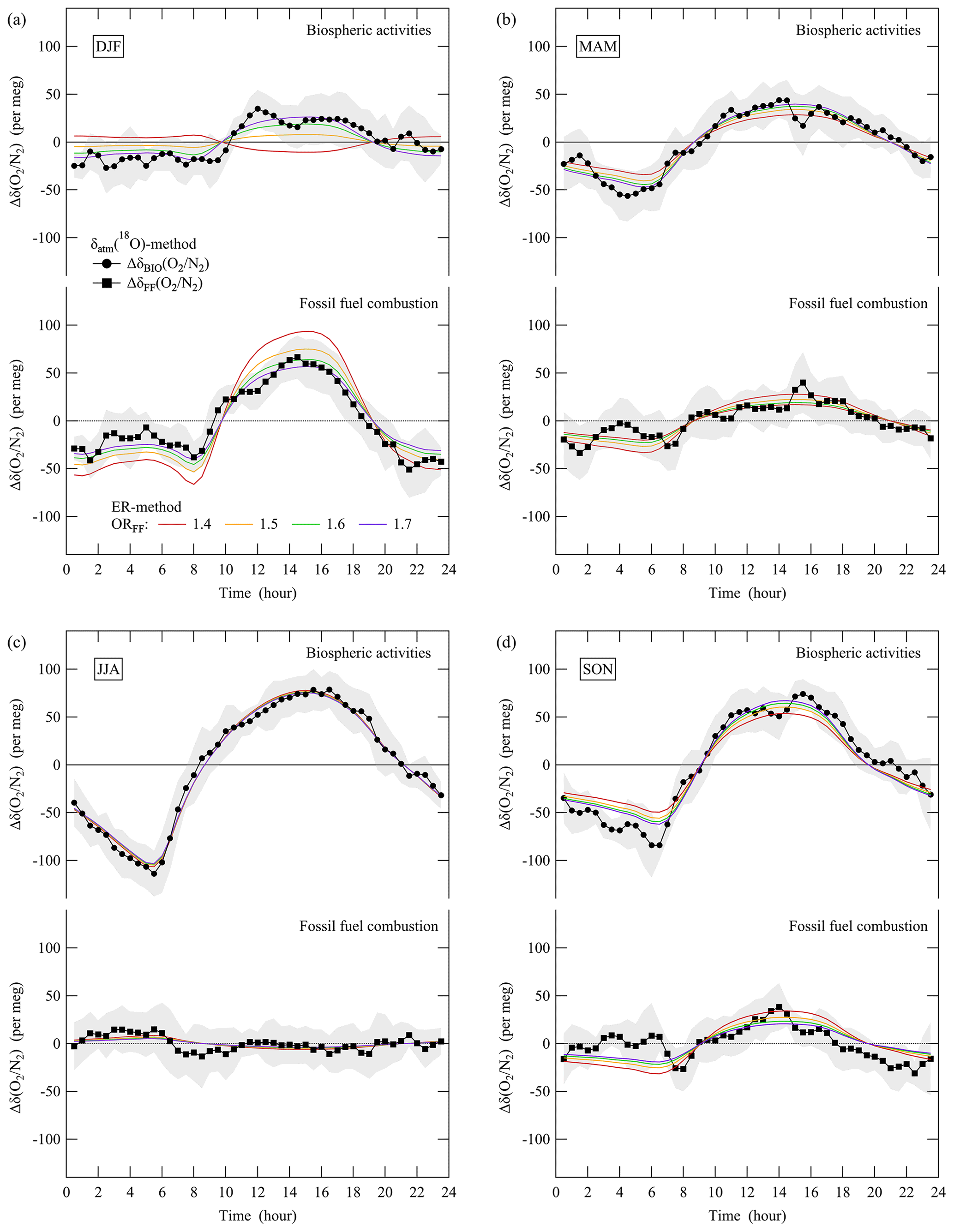
Figure 5 (a) Plots of the average diurnal cycles of Δδ_BIO(${\mathrm{O}}_{\mathrm{2}}/{\mathrm{N}}_{\mathrm{2}}$) and Δδ_FF(${\mathrm{O}}_{\mathrm{2}}/{\mathrm{N}}_{\mathrm{2}}$) for each season estimated by the δ_atm(¹⁸O) method. Δδ(${\mathrm{O}}_{\mathrm{2}}/{\mathrm{N}}_{\mathrm{2}}$) values driven by activities in the terrestrial biosphere and fossil fuel combustion estimated by the ER method are also shown. See the text for details of the δ_atm(¹⁸O) and ER methods. Δ denotes deviations from the diurnal mean values. Error bands for Δδ_BIO(${\mathrm{O}}_{\mathrm{2}}/{\mathrm{N}}_{\mathrm{2}}$) are derived from Δδ_atm(¹⁸O) in Fig. 4a. Error bands for Δδ_FF(${\mathrm{O}}_{\mathrm{2}}/{\mathrm{N}}_{\mathrm{2}}$) are assumed to be the same as those for Δδ_BIO(${\mathrm{O}}_{\mathrm{2}}/{\mathrm{N}}_{\mathrm{2}}$).

The equations for the ER method can be written as

$$\begin{array}{}\text{(6)}& {\displaystyle }\mathrm{\Delta }y\left({\mathrm{CO}}_{\mathrm{2}},\mathrm{B}\right)+\mathrm{\Delta }y\left({\mathrm{CO}}_{\mathrm{2}},\mathrm{FF}\right)=\mathrm{\Delta }y\left({\mathrm{CO}}_{\mathrm{2}}\right),\text{(7)}& {\displaystyle \frac{\mathrm{\Delta }y\left({\mathrm{CO}}_{\mathrm{2}},\mathrm{B}\right)\times {\mathit{\alpha }}_{\mathrm{B}}+\mathrm{\Delta }y\left({\mathrm{CO}}_{\mathrm{2}},\mathrm{FF}\right)\times {\mathit{\alpha }}_{\mathrm{F}}}{\mathrm{\Delta }y\left({\mathrm{CO}}_{\mathrm{2}},\mathrm{B}\right)+\mathrm{\Delta }y\left({\mathrm{CO}}_{\mathrm{2}},\mathrm{FF}\right)}}={\mathit{\alpha }}_{\mathrm{obs}}.\end{array}$$

Here, Δy(CO₂, B) and Δy(CO₂, FF) are changes in the amount fraction of CO₂ driven by terrestrial biosphere activities and fossil fuel combustion, respectively. Δy(CO₂) is the observed average diurnal cycle of the amount fraction of CO₂ for each season shown in Fig. 4a. α_B, α_F, and α_obs are the OR_B, OR_FF, and observed ER for each season shown in Fig. 4c. Once Δy(CO₂, B) and Δy(CO₂, FF) are calculated by solving Eqs. (5) and (6), they can be converted to Δδ(${\mathrm{O}}_{\mathrm{2}}/{\mathrm{N}}_{\mathrm{2}}$) by using OR_B and OR_FF, respectively.

Figure 5 shows the δ(${\mathrm{O}}_{\mathrm{2}}/{\mathrm{N}}_{\mathrm{2}}$) driven by terrestrial biosphere activities and fossil fuel combustion estimated by the ER method. The results agreed well with the δ_BIO(${\mathrm{O}}_{\mathrm{2}}/{\mathrm{N}}_{\mathrm{2}}$) and δ_FF(${\mathrm{O}}_{\mathrm{2}}/{\mathrm{N}}_{\mathrm{2}}$) for all seasons, especially when we chose the OR_FF to be 1.6 or 1.7, which are higher and lower than those expected from liquid fuel and natural gas fuel combustion, respectively. The implication is therefore that the diurnal δ_FF(${\mathrm{O}}_{\mathrm{2}}/{\mathrm{N}}_{\mathrm{2}}$) cycles at TKB were driven by car traffic (liquid fuels) and household gas consumption. It is noteworthy that propane (CH₃CH₂CH₃), for which the OR_FF is 1.67 assuming complete combustion, should also be considered a household gas consumed in the TKB area.

To determine whether variations of δ_atm(¹⁸O) on hourly to daily time frames were observable, we plotted typical examples in Fig. 6 of rolling averages calculated over 300 cycles (5 h) and 1100 cycles (19 h) of mass spectrometric measurements of δ_atm(¹⁸O) and δ(${\mathrm{O}}_{\mathrm{2}}/{\mathrm{N}}_{\mathrm{2}}$). The summertime graphs (Fig. 6a) clearly show that the δ_atm(¹⁸O) varied in antiphase with δ(${\mathrm{O}}_{\mathrm{2}}/{\mathrm{N}}_{\mathrm{2}}$) on timescales of both 5 and 19 h. The ratios of ${\mathit{\delta }}_{\mathrm{atm}}{(}^{\mathrm{18}}\mathrm{O})/\mathit{\delta }$(${\mathrm{O}}_{\mathrm{2}}/{\mathrm{N}}_{\mathrm{2}}$) were −0.017 per meg (per meg)⁻¹ for data averaged over both 5 and 19 h. This result agreed with that obtained from the summertime average diurnal cycle (vide supra). In contrast, there was no clear correlation between variations of δ_atm(¹⁸O) and δ(${\mathrm{O}}_{\mathrm{2}}/{\mathrm{N}}_{\mathrm{2}}$) in winter (Fig. 6b). We could distinguish some short-term δ_atm(¹⁸O) variations (Fig. 6b), but the causes were unclear. The variations may be partly due to activities in the biosphere because the δ_atm(¹⁸O) in winter showed small but substantial diurnal cycles of δ_atm(¹⁸O) and δ_BIO(${\mathrm{O}}_{\mathrm{2}}/{\mathrm{N}}_{\mathrm{2}}$) (Figs. 4a and 5a). These characteristics suggest that we could apply the δ_atm(¹⁸O) method to resolve temporal variations of δ_BIO(${\mathrm{O}}_{\mathrm{2}}/{\mathrm{N}}_{\mathrm{2}}$) and δ_FF(${\mathrm{O}}_{\mathrm{2}}/{\mathrm{N}}_{\mathrm{2}}$) separately on time frames of several hours to day to day. Similar separation has been carried out for CO₂ based on the simultaneous analysis of the Δ(¹⁴C) and amount fraction of CO₂(e.g., Graven et al., 2018; Basu et al., 2016, 2020) or based on the simultaneous analysis of δ(${\mathrm{O}}_{\mathrm{2}}/{\mathrm{N}}_{\mathrm{2}}$) and the amount fraction of CO₂ by assuming an average OR_FF based on a statistical assessment (e.g., Minejima et al., 2012; Sugawara et al., 2021; Pickers et al., 2022). The δ_atm(¹⁸O) method may have some advantages compared with methods used in previous studies because we could apply it without assuming any OR_FF with a temporal resolution of 5 h or perhaps even shorter.

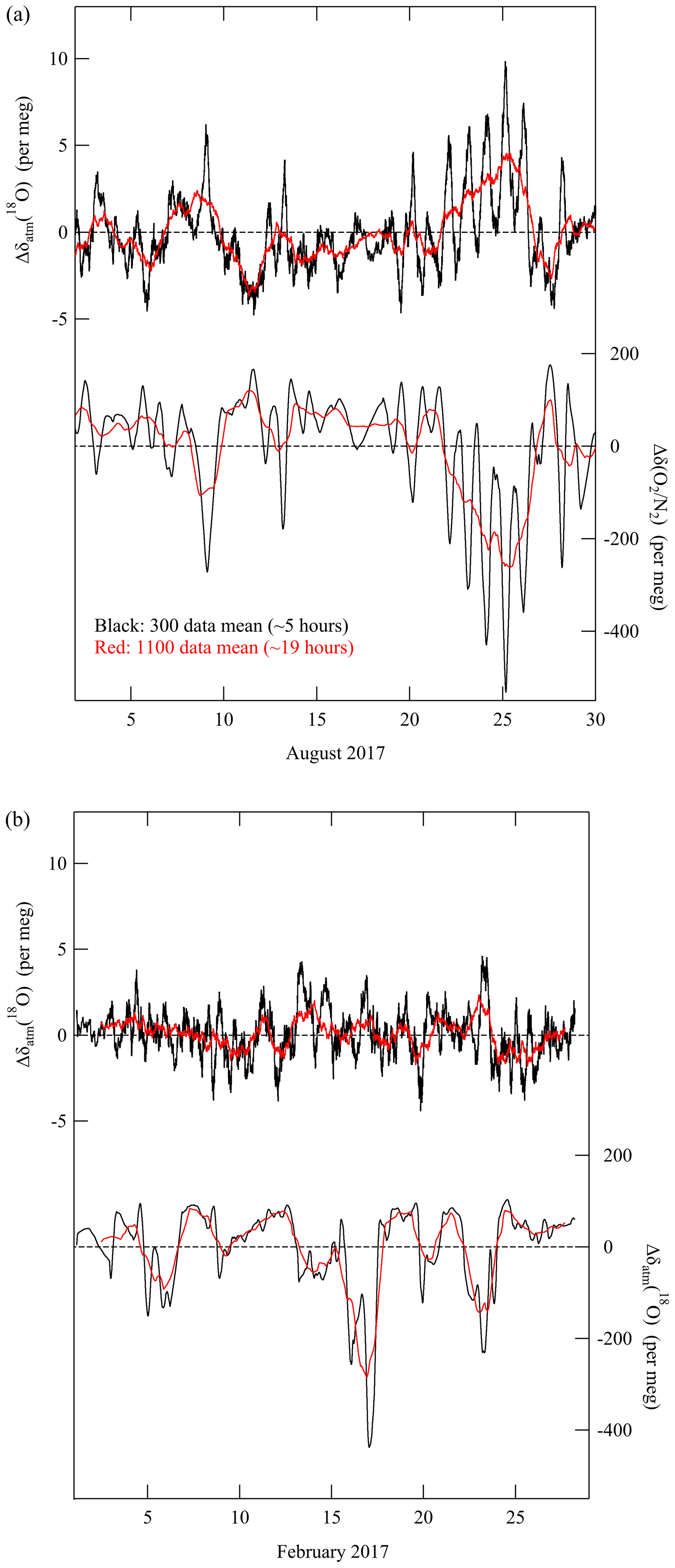
Figure 6 (a) Rolling average values of Δδ_atm(¹⁸O) and Δδ(${\mathrm{O}}_{\mathrm{2}}/{\mathrm{N}}_{\mathrm{2}}$) for 300 data points (black) and 1100 data points (red) at TKB in August 2017. Δ denotes deviations from the monthly mean value. (b) Same as in (a), but for February 2017.

3.2 Seasonal cycles of δ_atm(¹⁸O) and δ(${\mathrm{O}}_{\mathrm{2}}/{\mathrm{N}}_{\mathrm{2}}$)

Figure 7a shows the monthly mean values of δ_atm(¹⁸O) and δ(${\mathrm{O}}_{\mathrm{2}}/{\mathrm{N}}_{\mathrm{2}}$) at TKB during 2013–2022. To reduce local effects of fossil fuel combustion around TKB, we extracted the successive maxima of δ(${\mathrm{O}}_{\mathrm{2}}/{\mathrm{N}}_{\mathrm{2}}$) for 4320 cycles (3 d) of mass spectrometric measurements to calculate the monthly mean values of δ(${\mathrm{O}}_{\mathrm{2}}/{\mathrm{N}}_{\mathrm{2}}$) plotted in Fig. 7a. In contrast, all data were used to calculate the monthly mean values of δ_atm(¹⁸O) to reduce their standard errors because fossil fuel combustion did not change δ_atm(¹⁸O) significantly, as discussed in Sect. 3.1. We removed anomalous δ_atm(¹⁸O) data from the plot during 4 months when the mass spectrometer was producing unreliable results. Therefore, Fig. 7a shows 116 and 120 data points for δ_atm(¹⁸O) and δ(${\mathrm{O}}_{\mathrm{2}}/{\mathrm{N}}_{\mathrm{2}}$), respectively. Some seasonal and interannual variations are apparent in Fig. 7a, not only for δ(${\mathrm{O}}_{\mathrm{2}}/{\mathrm{N}}_{\mathrm{2}}$), which has been reported in many past studies (Keeling and Manning, 2014), but also for δ_atm(¹⁸O). We examined the observed average seasonal cycle and secular trend of δ_atm(¹⁸O), and in the following paragraphs we discuss the implications thereof for the oxygen, carbon, and water cycles.

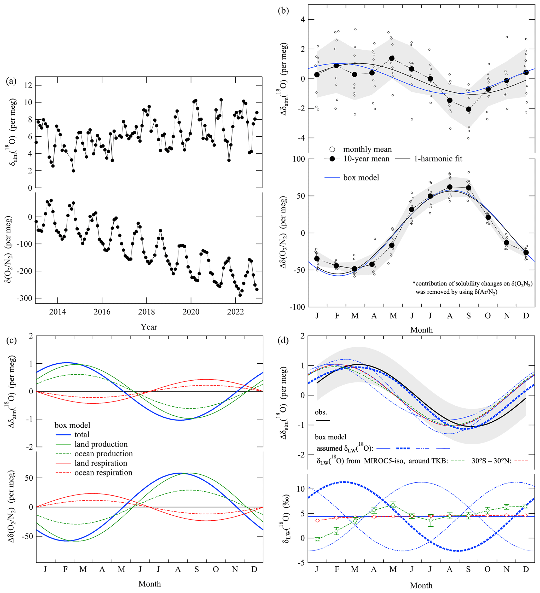
Figure 7 (a) Monthly mean values of δ_atm(¹⁸O) and δ(${\mathrm{O}}_{\mathrm{2}}/{\mathrm{N}}_{\mathrm{2}}$) observed at TKB for the period 2013–2022. Local effects of fossil fuel combustion around TKB were excluded from δ(${\mathrm{O}}_{\mathrm{2}}/{\mathrm{N}}_{\mathrm{2}}$). See the text for details. (b) Detrended monthly mean values (open black circles) and their 10-year average (filled black circles) of Δδ_atm(¹⁸O) at TKB for the period 2013–2022. Those of Δδ(${\mathrm{O}}_{\mathrm{2}}/{\mathrm{N}}_{\mathrm{2}}$), extracted by removing the contributions of solubility change by using the average seasonal δ($\mathrm{Ar}/{\mathrm{N}}_{\mathrm{2}}$) cycle at TKB (see text), are also shown. Average seasonal cycles of Δδ_atm(¹⁸O) and Δδ(${\mathrm{O}}_{\mathrm{2}}/{\mathrm{N}}_{\mathrm{2}}$) obtained by applying one-harmonic best-fit curves to the data (solid black lines) and those simulated by the box model (solid blue lines) are also shown. We assumed a constant δ_LW(¹⁸O) of 4.4 ‰ for the simulation. Δ denotes deviations from the annual mean values. (c) Same average seasonal cycles of Δδ_atm(¹⁸O) and Δδ(${\mathrm{O}}_{\mathrm{2}}/{\mathrm{N}}_{\mathrm{2}}$) simulated by the box model in (b) (solid blue lines), the contributions of terrestrial and ocean production (solid and dashed green lines, respectively), and terrestrial and ocean respiration (solid and dashed red lines, respectively). (d) The same best-fit curve for δ_atm(¹⁸O) as in (b). Error bands indicate average deviations from the 10-year average of Δδ_atm(¹⁸O) (±1σ). Same average seasonal cycle of Δδ_atm(¹⁸O) simulated by the box model as in (b) and corresponding δ_LW(¹⁸O) values (solid blue lines). Additional simulations of average seasonal Δδ_atm(¹⁸O) cycles and the incorporated seasonally varying δ_LW(¹⁸O) values for sensitivity tests (thick dashed blue line, dashed blue two-dot line, and dotted line), as well as those incorporating the average monthly δ_LW(¹⁸O) around TKB (36° N, 140° E) (green open circles) and at lower latitude (30° S–30° N) (red open circles) during 2013–2022 calculated by MIROC5-iso, are also shown (dashed green and red lines, respectively).

Figure 7b shows the average seasonal cycles of δ_atm(¹⁸O) and δ(${\mathrm{O}}_{\mathrm{2}}/{\mathrm{N}}_{\mathrm{2}}$) at TKB during 2013–2022. The δ(${\mathrm{O}}_{\mathrm{2}}/{\mathrm{N}}_{\mathrm{2}}$) values in this figure are the values after contributions from the solubility changes in the ocean were removed. For this purpose, we used the seasonal δ($\mathrm{Ar}/{\mathrm{N}}_{\mathrm{2}}$) cycle, which is driven mainly by the air–sea heat flux at the surface (e.g., Keeling et al., 2004; Ishidoya et al., 2021; Morgan et al., 2021). Specifically, the average seasonal cycle of δ($\mathrm{Ar}/{\mathrm{N}}_{\mathrm{2}}$) at TKB (Ishidoya et al., 2021), multiplied by a coefficient of 0.9 derived from differences in the solubilities of O₂ and Ar (Weiss, 1970), was subtracted from the average seasonal cycle of δ(${\mathrm{O}}_{\mathrm{2}}/{\mathrm{N}}_{\mathrm{2}}$). We applied this correction so that we could discuss the variations of δ(${\mathrm{O}}_{\mathrm{2}}/{\mathrm{N}}_{\mathrm{2}}$) associated with only the DME. The peak-to-peak amplitude of the corrected seasonal δ(${\mathrm{O}}_{\mathrm{2}}/{\mathrm{N}}_{\mathrm{2}}$) cycle was smaller than that of the uncorrected seasonal δ(${\mathrm{O}}_{\mathrm{2}}/{\mathrm{N}}_{\mathrm{2}}$) cycle by about 7 per meg. It is apparent in Fig. 7b that the δ_atm(¹⁸O) varied seasonally, roughly in antiphase with the seasonal cycle of δ(${\mathrm{O}}_{\mathrm{2}}/{\mathrm{N}}_{\mathrm{2}}$). The minimum of the seasonal δ_atm(¹⁸O) cycle appeared in late summer to early autumn, and the peak-to-peak amplitude was 2.1±0.6 per meg. The maximum of the seasonal δ(${\mathrm{O}}_{\mathrm{2}}/{\mathrm{N}}_{\mathrm{2}}$) cycle occurred in summer, and its peak-to-peak amplitude was 112±10 per meg. The uncertainties for the amplitudes of δ_atm(¹⁸O)(δ(${\mathrm{O}}_{\mathrm{2}}/{\mathrm{N}}_{\mathrm{2}}$)) were evaluated as a standard deviation of the 10-year average monthly mean values from the best-fit curve shown in Fig. 7b. Keeling (1995) expected δ_atm(¹⁸O) to be lower in summer than in winter by 2 per meg based on the assumption that the 100 per meg seasonal increase in δ(${\mathrm{O}}_{\mathrm{2}}/{\mathrm{N}}_{\mathrm{2}}$) was driven by the input of photosynthetic O₂, the δ(¹⁸O) of which is about 20 ‰ lower than δ_atm(¹⁸O). This can be calculated as

$$\begin{array}{}\text{(8)}& \mathit{\delta }{}_{\mathrm{atm}\mathrm{\_}\mathrm{summer}}\left({}^{\mathrm{18}}\mathrm{O}\right)={\displaystyle \frac{\begin{array}{c}\left(y{\left({\mathrm{O}}_{\mathrm{2}}\right)}_{\mathrm{winter}}\times \mathit{\delta }{}_{\mathrm{atm}\mathrm{\_}\mathrm{winter}}\left({}^{\mathrm{18}}\mathrm{O}\right)\right.\\ \left.+\mathrm{\Delta }y\left({\mathrm{O}}_{\mathrm{2}}\right)\times \mathit{\delta }{}_{\mathrm{LW}}\left({}^{\mathrm{18}}\mathrm{O}\right)\right)\end{array}}{y{\left({\mathrm{O}}_{\mathrm{2}}\right)}_{\mathrm{winter}}+\mathrm{\Delta }y\left({\mathrm{O}}_{\mathrm{2}}\right)}}.\end{array}$$

Here, δ_{atm_summer}(¹⁸O) and δ_{atm_winter}(¹⁸O) are δ_atm(¹⁸O) in summer and winter, respectively, y(O₂)_winter is the atmospheric O₂ amount fraction in winter, and Δy(O₂) is an input of photosynthetic O₂ to the atmosphere. If we assume δ_{atm_winter}(¹⁸O) and δ_LW(¹⁸O) are 0 ‰ and −20 ‰, respectively, y(O₂)_winter is 209 400 µmol mol⁻¹, and Δy(O₂) is 21 µmol mol⁻¹, which corresponds to a 100 per meg seasonal increase in δ(${\mathrm{O}}_{\mathrm{2}}/{\mathrm{N}}_{\mathrm{2}}$), then we obtain δ_{atm_summer}(¹⁸O) of −2 per meg as in Keeling (1995). Although his estimation was relatively simple, it reproduced the general characteristics of the seasonal δ_atm(¹⁸O) and δ(${\mathrm{O}}_{\mathrm{2}}/{\mathrm{N}}_{\mathrm{2}}$) cycles observed in the present study well. In Fig. 7b, we also plot the seasonal cycles of δ_atm(¹⁸O) and δ(${\mathrm{O}}_{\mathrm{2}}/{\mathrm{N}}_{\mathrm{2}}$) simulated by our box model that incorporated the isotopic effects from B94. The R_Res, R_PS, R_OR, and R_OP values in the model were adjusted to reproduce the observed seasonal δ(${\mathrm{O}}_{\mathrm{2}}/{\mathrm{N}}_{\mathrm{2}}$) cycle by imposing the constraints that the annual average $R_{\mathrm{Res}}=-R_{\mathrm{PS}}$ and $R_{\mathrm{OR}}=-R_{\mathrm{OP}}$. We then adjusted the initial value of the δ_atm(¹⁸O) in the model arbitrarily to establish a steady state for the simulated δ_atm(¹⁸O). We set the $R_{\mathrm{Res}}/R_{\mathrm{OR}}$(or $R_{\mathrm{PS}}/R_{\mathrm{OP}}$) ratio to be 2 for the simulation in Fig. 7b. As discussed in Sect. 3.1, changes in that ratio do not substantially change the simulated results of δ_atm(¹⁸O). Figure 7c shows the same simulated seasonal cycles of δ_atm(¹⁸O) and δ(${\mathrm{O}}_{\mathrm{2}}/{\mathrm{N}}_{\mathrm{2}}$) in Fig. 7b and the respective contributions of terrestrial production, terrestrial respiration, ocean production, and ocean respiration. As seen from Fig. 7c, the seasonal δ_atm(¹⁸O) cycle is driven mainly by production rather than respiration, which is consistent with the estimation by Keeling (1995). In this context, seasonal cycles of ${\mathit{\delta }}_{{\mathrm{CO}}_{\mathrm{2}}}{(}^{\mathrm{18}}\mathrm{O})$ have been reported by some past studies (e.g., Peylin et al., 1999; Cuntz et al., 2003; Murayama et al., 2010). Peylin et al. (1999) and Cuntz et al. (2003) used 3D atmospheric transport models to reproduce the observations, and they found that the main contributors are respiration and production for the respective seasonal cycles of ${\mathit{\delta }}_{{\mathrm{CO}}_{\mathrm{2}}}{(}^{\mathrm{18}}\mathrm{O})$ and CO₂ amount fraction. These characteristics are different from the seasonal cycles of δ_atm(¹⁸O) and δ(${\mathrm{O}}_{\mathrm{2}}/{\mathrm{N}}_{\mathrm{2}}$) observed in this study, both of which are driven mainly by production (Fig. 7c).

We found that the box model could reproduce the observed seasonal δ_atm(¹⁸O) cycles, although both the seasonal minimum and maximum of the simulated seasonal δ_atm(¹⁸O) cycle appeared slightly earlier (by about 1 month) than in the observed cycle represented by a one-harmonic, best-fit curve (Fig. 7b). A 1- to 2-month time shift between the observed and simulated seasonal cycles is also found in ${\mathit{\delta }}_{{\mathrm{CO}}_{\mathrm{2}}}{(}^{\mathrm{18}}\mathrm{O})$ at various surface stations (Peylin et al., 1999; Cuntz et al., 2003), although the box model used in this study is much more primitive compared to the 3D models in past studies. To investigate the possible cause(s) of the phase difference, we carried out additional simulations that incorporated three different seasonally varying δ_LW(¹⁸O) values into the box model.

Figure 7d shows the simulated results along with the one-harmonic, best-fit curve to the observed data. It is apparent from this figure that the appearance of the seasonal minimum and maximum of δ_atm(¹⁸O) depended on the seasonal variations of δ_LW(¹⁸O). It is also apparent that the observed seasonal cycle of δ_atm(¹⁸O) was well reproduced by the simulation that incorporated the δ_LW(¹⁸O) represented by the thick dashed blue line. The scenario for the thick dashed blue line was determined based on some past studies that reported seasonal variations of δ_LW(¹⁸O) (e.g., Welp et al., 2008; Plavcová et al., 2018; Cernusak et al., 2022; Liu et al., 2023), and two other scenarios represented by a two-dot line and dotted lines were carried out as sensitivity tests to the phase difference in the seasonal δ_LW(¹⁸O) cycle. Welp et al. (2008) observed the time series of ecosystem water pools at a soybean canopy in Minnesota, USA, from 30 May to 27 September 2006 and found the most extreme enrichment of bulk δ_LW(¹⁸O) to be 20 ‰ above xylem water during the early part of the growing season (Fig. 1a in Welp et al., 2008). Plavcová et al. (2018) and Liu et al. (2023) also reported less enrichment of δ_LW(¹⁸O) toward the end of the vegetation season by about 10 ‰–20 ‰, and Cernusak et al. (2022) reported a strong negative correlation between the δ_LW(¹⁸O) and the relative humidity of air based on a recent global meta-analysis. These characteristics are roughly consistent with the δ_LW(¹⁸O) represented by the thick dashed blue line in Fig. 7d, which shows decreases in δ_LW(¹⁸O) toward the end of the vegetation season similar in magnitude to decreases reported in past studies. In this regard, Murayama et al. (2010) observed ${\mathit{\delta }}_{{\mathrm{CO}}_{\mathrm{2}}}{(}^{\mathrm{18}}\mathrm{O})$ at a forest site in Japan and reported that monthly mean ${\mathit{\delta }}_{{\mathrm{CO}}_{\mathrm{2}}}{(}^{\mathrm{18}}\mathrm{O})$ correlated positively with δ(¹⁸O) of precipitation (δ_precip(¹⁸O)). Since variations in δ_LW(¹⁸O) are closely related to those in δ_precip(¹⁸O), it is suggested that δ_LW(¹⁸O) is an important driver in modifying seasonal cycles for both δ_atm(¹⁸O) and ${\mathit{\delta }}_{{\mathrm{CO}}_{\mathrm{2}}}{(}^{\mathrm{18}}\mathrm{O})$.

We also carried out additional box model simulations that incorporated the average monthly δ_LW(¹⁸O) around TKB (36° N, 140° E) and at lower latitude (30° S–30° N) calculated by MIROC5-iso for the period 2013–2022. The results are plotted in Fig. 7d, and both the monthly δ_LW(¹⁸O) and simulated seasonal δ_atm(¹⁸O) cycles fall within the range of those represented by the blue two-dot lines and dotted lines in the figure discussed above. Another factor in changing the simulated seasonal δ_atm(¹⁸O) cycle is the choice of the isotopic effects from B94 or L&B11 (Table 1). If we use the isotopic effects from L&B11 and ignore R_Res and R_PS(i.e., we consider marine respiration and production only), then the seasonal amplitude of the simulated δ_atm(¹⁸O) increases by 20 % compared with that simulated by using the isotopic effects from B94. This is due to the difference in the isotopic effects of ocean respiration, which are 18.9 ‰ and 23.5 ‰ for B94 and L&B11, respectively. Such a difference will become apparent in the Southern Hemisphere, where the seasonal δ(${\mathrm{O}}_{\mathrm{2}}/{\mathrm{N}}_{\mathrm{2}}$) cycle is driven mainly by the air–sea O₂ flux (e.g., Keeling and Manning, 2014). Therefore, spatiotemporal variations in the seasonal δ_atm(¹⁸O) cycle will be useful to constrain not only spatiotemporal variations of δ_LW(¹⁸O) but also the isotopic effects of ocean respiration.

3.3 Secular trend in δ_atm(¹⁸O)

Figure 8 shows temporal changes in the annual average δ_atm(¹⁸O) observed at TKB. The error band denotes the ±0.9 per meg of the long-term stability of δ_atm(¹⁸O) in our standard air (Fig. 2). It is apparent in Fig. 8a that the δ_atm(¹⁸O) underwent a slight secular increase of (0.22±0.14) per meg a⁻¹ throughout the observation period. This rate was calculated from the difference between the 2013 and 2022 annual average δ_atm(¹⁸O), and the uncertainty around the long-term stability was taken into account. The observed secular increasing trend was quite different from the secular decrease in the DME expected by Seibt et al. (2005), which was on the order of 70 per meg over the last 150 years (−0.5 per meg a⁻¹). They calculated the secular change by assuming anthropogenic changes in the terrestrial oxygen cycle from pre- to post-industrial times: (1) a replacement of 3 % of terrestrial respiratory O₂ release by biomass burning, (2) a 5 % decrease in global terrestrial GPP, (3) a decrease in global photorespiration due to the increase in the amount fraction of atmospheric CO₂ by 100 µmol mol⁻¹, (4) a 10 % decrease in stomatal conductance resulting from CO₂ increases and a partial offset of photorespiratory decreases, and (5) a 5 % decrease in the O₂-flux-weighted ¹⁸O enrichment of foliage water due to higher contributions of ¹⁸O-depleted northern midlatitude biomes. The fact that the observation period of 10 years in the present study was much shorter than the 150 years discussed in Seibt et al. (2005) makes it difficult to discuss the significance of the difference between the secular trends in the two studies. It would nevertheless be of interest to see if the observed secular trend could be reproduced using our box model. In that case we could explore the applicability of the precise observations of the δ_atm(¹⁸O).

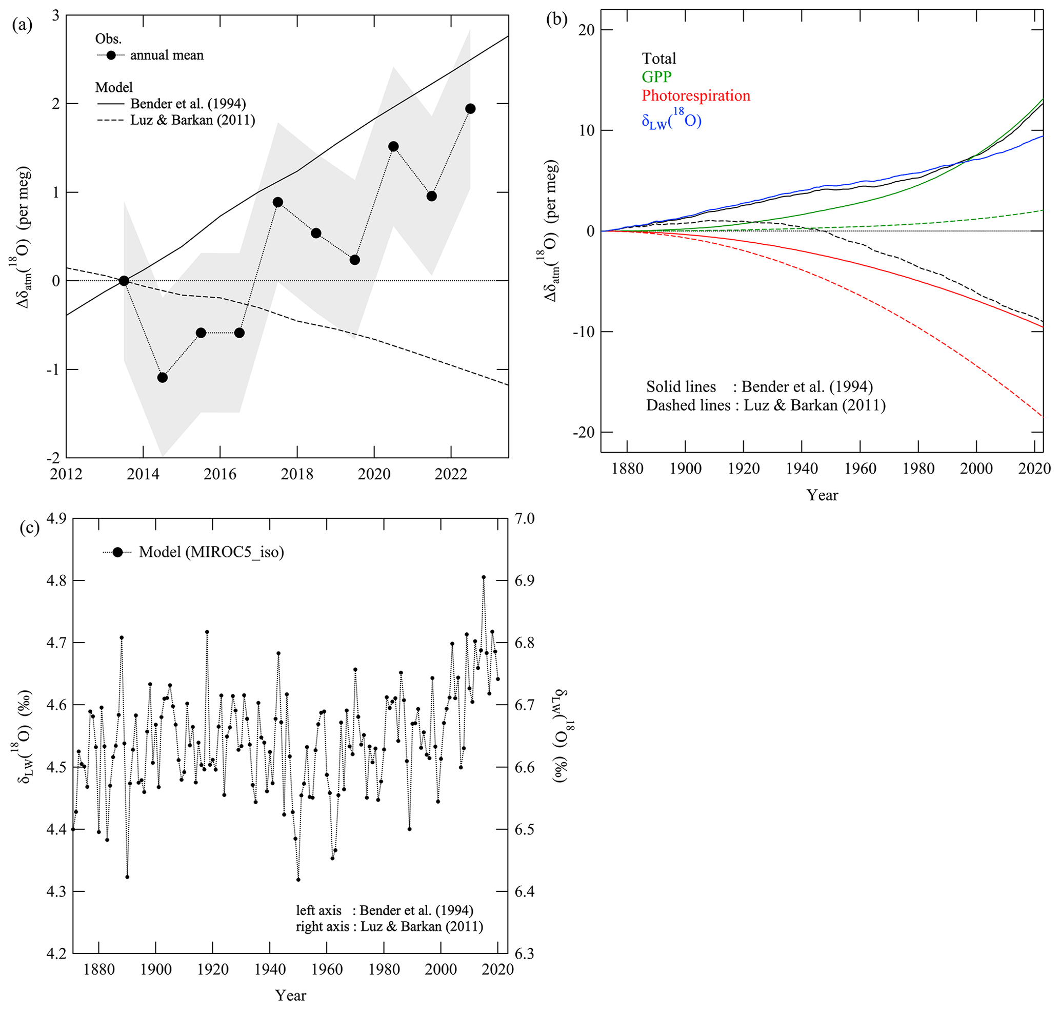
Figure 8 (a) Annual average values of Δδ_atm(¹⁸O) observed at TKB (filled circles). Δδ_atm(¹⁸O) simulated by the box model for the period 2012–2022, assuming the isotopic effects reported by Bender et al. (1994) (solid line) and Luz and Barkan (2011) (dashed line). Δ denotes deviations from the observed value in 2013. See the text for details. (b) Same Δδ_atm(¹⁸O) simulated by the box model but for data during 1871–2022 and the respective contributions of the changes in GPP (green line), photorespiration (red line), and δ_LW(¹⁸O) (blue line) to the simulated δ_atm(¹⁸O). Solid and dashed lines denote the simulated data assuming the isotopic effects reported by Bender et al. (1994) and Luz and Barkan (2011), respectively. The solid and dashed blue lines almost overlap. Δ denotes deviations from the simulated value in 1871. (c) Annual average values of the global average δ_LW(¹⁸O) calculated by MIROC5-iso. The values in 1871 were arbitrarily adjusted to 4.4 (left axis) or 6.5 ‰ (right axis), respectively, for the DME at steady state by Bender et al. (1994) or Luz and Barkan (2011).

To explore that possibility, we carried out calculations in which we assumed that there were long-term changes in (1) GPP, (2) photorespiration, and (3) δ_LW(¹⁸O). Note that we considered long-term changes in only terrestrial fluxes for the GPP and photorespiration. Changes in marine photosynthetic and respiratory O₂ fluxes should be included in more detailed future studies.

We first assumed that the global terrestrial GPP increases in proportion to the global average CO₂ amount fraction. As the global average CO₂ amount fraction, we used data from the Scripps CO₂ Program (https://scrippsco2.ucsd.edu/data/atmospheric_co2/icecore_ merged_products.html, last access: 21 August 2024) based on ice core data and direct observations before and after 1959, respectively (Keeling et al., 2001; Rubino et al., 2019). We assume the initial terrestrial production of O₂ in 1871 to be 16.7 Pmol a⁻¹(Table 1), which corresponds to 107 Pg a⁻¹(C equivalents) of global terrestrial GPP considering the r_DR of 0.59 and the OR_B of 1.1. Then, the GPP increased secularly with increasing CO₂ amount fraction, and it was 141 Pg a⁻¹(C equivalents) in 2006. Although this is somewhat larger than the average GPP of 125 Pg a⁻¹(C equivalents) for the period 1992–2020 reported by Bi et al. (2022), it falls within a range of the global GPP estimates from various models summarized in Fig. 10 of Zheng et al. (2020). A similar increase in global GPP during the 20th century has also been reported by Campbell et al. (2017) based on long-term atmospheric carbonyl sulfide (COS) records derived from ice core, firn, and ambient air samples.

Second, we assumed an increase of 120 µmol mol⁻¹ in the amount fraction of atmospheric CO₂ during the 150 years from pre-industrial times to the present. This increase caused a decrease in global average photorespiration based on Farquhar et al. (1980):

$$\begin{array}{}\text{(9)}& \begin{array}{rl}\mathit{\varphi }& =\left(V_{\mathrm{O}\mathrm{\_}\max }/V_{\mathrm{C}\mathrm{\_}\max }\right)\times \left(y\left({\mathrm{O}}_{\mathrm{2}}\right)/y\left({\mathrm{CO}}_{\mathrm{2}}\right)\right)\\ & \times \left(K_{\mathrm{C}}/K_{\mathrm{O}}\right)\times {\mathrm{10}}^{-\mathrm{3}},\end{array}\end{array}$$

where ϕ is the ratio of photorespiration to carboxylation (or total carbon fixation, the amount of which corresponds to the sum of GPP, photorespiration, and the Mehler reaction), and ($V_{\mathrm{O}\mathrm{\_}\max }/V_{\mathrm{C}\mathrm{\_}\max }$) is the ratio of the maximum oxygenation velocity to the maximum carboxylation velocity of RuP₂ carboxylase–oxygenase (we used 0.21 for this ratio from Eq. 16 in Farquhar et al., 1980). y(O₂) and y(CO₂) are amount factions of O₂ and CO₂, respectively, in equilibrium with their dissolved amount fractions in the chloroplast stroma. We used atmospheric y(O₂) and atmospheric y(CO₂) multiplied by 0.7 following B94. ($K_{\mathrm{C}}/K_{\mathrm{O}}$) is the ratio of the Michaelis–Menten constants for carboxylation and oxygenation, respectively (we adopted 460 $/$ 330 for this ratio from Table 1 in Farquhar et al., 1980). 10⁻³ is a coefficient to compare the calculated ϕ values with those in Farquhar et al. (1980) directly since they used units of millibars (mbar) and microbars (µbar) for y(O₂) and y(CO₂), respectively. We calculated ϕ to be 0.31 and 0.22 for CO₂ amount fractions of 280 and 400 µmol mol⁻¹, respectively.

We then calculated changes in δ_LW(¹⁸O) with MIROC5-iso for the period 1871–2022. We considered the water cycle to be in steady state before 1871, and we assumed the global average δ_LW(¹⁸O) in 1871 to be 4.4 ‰ or 6.5 ‰ based on previous studies for the DME in steady state by B94 or L&B11, respectively. In this connection, Hoffmann et al. (2004) reported an intermediate δ_LW(¹⁸O) of 5 ‰–6 ‰. It should be noted that the original δ_LW(¹⁸O) calculated by MIROC5-iso for 1871 was about −0.7 ‰, so we arbitrarily shifted all δ_LW(¹⁸O) values calculated by MIROC5-iso by 5.1 ‰ or 7.2 ‰. Clarifying the cause(s) of the low δ_LW(¹⁸O) calculated by MIROC5-iso will be a future task. Figure 8c shows the global average δ_LW(¹⁸O); δ_LW(¹⁸O) underwent a significant secular increase throughout the period. The increase was especially clear after the 1980s, which is the time when there was an increase in the δ_precip(¹⁸O) simulated by MIROC5-iso (not shown). Rozanski et al. (1992) reported that δ_precip(¹⁸O) increases with increasing surface air temperature by 0.6 ‰ K⁻¹, and the global average surface air temperature has increased by about 1 K from 1980 to the present. The increase in surface air temperature has therefore caused at least part of the simulated secular increase in δ_LW(¹⁸O) since 1980. Previous studies have also reported that a lower (larger) relative humidity near the plant stomata enhances (diminishes) δ_LW(¹⁸O) (Eq. 2 of Hoffmann et al., 2004). Also, Byrne and O'Gorman (2018) reported that the relative humidity over land from 40° S to 40° N has decreased secularly since 1980. It is therefore possible that the decrease in relative humidity also contributed to the simulated secular increase in δ_LW(¹⁸O) since 1980. It should be noted that Welp et al. (2011) suggested that ${\mathit{\delta }}_{{\mathrm{CO}}_{\mathrm{2}}}{(}^{\mathrm{18}}\mathrm{O})$ increases with increasing δ_precip(¹⁸O) and δ_LW(¹⁸O) through the redistribution of moisture and rainfall in the tropics during an El Niño, which leads to substantial interannual variations in ${\mathit{\delta }}_{{\mathrm{CO}}_{\mathrm{2}}}{(}^{\mathrm{18}}\mathrm{O})$ during 1977–2009 obtained from the Scripps Institution of Oceanography global flask network. Therefore, it will be important in future studies to examine not only the secular trend discussed in this study but also interannual variations in δ_LW(¹⁸O) and δ_atm(¹⁸O).

Figure 8a and b show δ_atm(¹⁸O) simulated by the box model that incorporated the abovementioned long-term changes in GPP, photorespiration, and δ_LW(¹⁸O). The observed and simulated secular trends in δ_atm(¹⁸O) agreed well with each other under the conditions assuming the isotopic effects from B94. On the other hand, the simulated δ_atm(¹⁸O) assuming the isotopic effects from L&B11 decreased secularly, contrary to the observed secular increase. Figure 8b shows the respective contributions of the changes in GPP, photorespiration, and δ_LW(¹⁸O) to the simulated δ_atm(¹⁸O). The simulated δ_atm(¹⁸O) showed secular increases with increasing GPP during 1871–2023, and the increase is much larger in the simulation assuming the isotopic effects from B94 than that from L&B11. The simulated δ_atm(¹⁸O) showed secular increases with increasing δ_LW(¹⁸O) for both the cases assuming isotopic effects from B94 and L&B11. This pattern differed from the results simulated by Seibt et al. (2005), who reported a secular decrease in δ_atm(¹⁸O) based on assumed secular decreases in GPP and δ_LW(¹⁸O) during the last 150 years. It is noted that the contributions of the changes in δ_LW(¹⁸O) to the simulated δ_atm(¹⁸O) increased with time monotonously, while a clear increase in δ_LW(¹⁸O) was found after the 1980s (Fig. 8b–c). This is due to the choice of the initial δ_LW(¹⁸O) in 1871; we set it to be 4.4 ‰ or 6.5 ‰ (the values for steady state by B94 or L&B11). As seen from Fig. 8c, the average δ_LW(¹⁸O) during 1872–1980 was higher than the initial values, which made the monotonous increase in δ_atm(¹⁸O) driven by the δ_LW(¹⁸O) changes. In contrast, both the present study and that of Seibt et al. (2005) found a secular decrease in the simulated δ_atm(¹⁸O) with a decreasing ratio of photorespiration to carboxylation (ϕ).

The contributions of ϕ and δ_LW(¹⁸O) almost canceled each other in the simulation assuming the isotopic effects from B94. As a result, the simulated δ_atm(¹⁸O) based on B94 increased secularly due mainly to the contribution of the secular increase in GPP. On the other hand, the contribution of GPP to the simulated δ_atm(¹⁸O) assuming the isotopic effects from L&B11 is much smaller. Moreover, the secular decrease in the simulated δ_atm(¹⁸O) due to the contribution of ϕ is larger for the simulation assuming the isotopic effects from L&B11 than that from B94. As a result, the simulated δ_atm(¹⁸O) based on L&B11 decreased secularly due mainly to the contribution of the secular decrease in ϕ. The substantial differences between the contributions of GPP for the simulations based on B94 and L&B11 are attributed to the differences in the terrestrial and oceanic DME in their studies. Specifically, the respective terrestrial and oceanic DMEs in steady state are 22.4 ‰ and 18.9 ‰ in B94, while they are 23.5 ‰ and 23.5 ‰ in L&B11 (Table 1). Therefore, the secular increase in terrestrial production incorporated into our simulations led to the secular increase in δ_atm(¹⁸O) for the isotopic effects based on B94. The substantial difference in the contributions of ϕ, found between the simulations based on B94 and L&B11, is attributed to the increase in r_DR accompanied by a decrease in ϕ and the larger isotopic effect for dark respiration in B94 (18 ‰) than that in L&B11 (15.8 ‰). Therefore, we confirmed that secular trends in the simulated δ_atm(¹⁸O) are highly sensitive to the isotopic effects associated with the DME. This means that further studies are needed to determine the isotopic effects precisely in order to evaluate long-term changes in GPP and photorespiration based on δ_atm(¹⁸O). In this regard, some past studies evaluated the mechanisms responsible for the increase in global GPP. For example, Madani et al. (2020) reported an increase in GPP in northern latitudes caused by a reduction of cold-temperature constraints on plant growth. This scenario suggests that there has been an increase in negative carbon–climate feedback in high latitudes, whereas there has been a suggestion of an emerging positive climate feedback in the tropics, mainly due to an increase in the atmospheric vapor pressure deficit. They also pointed out that models have been struggling to determine how much additional CO₂ is being taken up by plants as a result of increased amount fractions of atmospheric CO₂. Therefore, an analysis based on a secular change in δ_atm(¹⁸O), which enables estimation of changes in the ratios of carboxylation to global GPP and photorespiration to global GPP, will facilitate better understanding of global CO₂ fertilization processes.

We used the global average secular change in δ_LW(¹⁸O) simulated by MIROC5-iso in this analysis, and we found that it made a substantial contribution to the simulated δ_atm(¹⁸O). The implication is that the secular change in the water cycle must be accurate before the observed and simulated secular trends of δ_atm(¹⁸O) can be equated. In other words, δ_atm(¹⁸O) is a unique tracer for a comprehensive evaluation of global changes in the oxygen, carbon, and water cycles. For example, if the secular increase in the global average amount fraction of atmospheric CO₂ stops without changes in the secular increasing trends of GPP, then the global average δ_atm(¹⁸O) will increase faster than the rate shown in Fig. 8a by assuming the isotopic effects from B94. A substantial secular decrease in the global average δ_atm(¹⁸O) may also be expected under pessimistic scenarios, such as substantial deforestation (secular decrease in GPP) and an increase in the average global amount fraction of atmospheric CO₂. In both cases, the results are regulated by climate changes such as changes in surface air temperature and aridification that lead to secular changes in δ_LW(¹⁸O).

We recognize that secular changes in stratospheric gravitational separation may cause slight secular changes in the surface δ_atm(¹⁸O). Ishidoya et al. (2021) estimated this effect for atmospheric δ($\mathrm{Ar}/{\mathrm{N}}_{\mathrm{2}}$) at the surface to be 0.15 and −0.13 per meg a⁻¹ when accompanied by a weakening or enhancement of the Brewer–Dobson circulation, respectively. These values correspond to 0.03 and −0.02 per meg a⁻¹, respectively, for δ_atm(¹⁸O) if mass-dependent gravitational separation is assumed. The secular trend of δ_atm(¹⁸O) due to changes in stratospheric gravitational separation is negligible at present because the changes are much smaller than the uncertainty of the secular trend of the observed δ_atm(¹⁸O) at TKB ((0.22 ± 0.14) per meg a⁻¹). If the observation period increases, the uncertainty of the secular trend will be smaller. Consideration of stratospheric gravitational separation changes may therefore be needed in the future.

4 Conclusions

We have carried out high-precision measurements of δ_atm(¹⁸O) at the TKB site since 2013. Clear variations of δ_atm(¹⁸O) with a daytime minimum were found for the average diurnal cycles throughout the observation period. The much larger amplitudes of the diurnal δ_atm(¹⁸O) cycles in summer than in winter suggest a substantial contribution of the activities in the terrestrial biosphere to the diurnal cycle. The amplitudes and phases of the diurnal δ_atm(¹⁸O) and δ(${\mathrm{O}}_{\mathrm{2}}/{\mathrm{N}}_{\mathrm{2}}$) cycles simulated by a box model, which incorporated the terrestrial oxygen cycle, were roughly consistent with the observed diurnal cycles in summer. Seasonal changes in the ERs, calculated from the average diurnal cycles of the δ(${\mathrm{O}}_{\mathrm{2}}/{\mathrm{N}}_{\mathrm{2}}$) and amount fractions of CO₂, also indicated a larger contribution of the activities in the terrestrial biosphere in summer than in winter. We found that the 5 h and 19 h averaged δ_atm(¹⁸O) also varied in antiphase with δ(${\mathrm{O}}_{\mathrm{2}}/{\mathrm{N}}_{\mathrm{2}}$) in summer. We found that the diurnal cycles of δ_BIO(${\mathrm{O}}_{\mathrm{2}}/{\mathrm{N}}_{\mathrm{2}}$) and δ_FF(${\mathrm{O}}_{\mathrm{2}}/{\mathrm{N}}_{\mathrm{2}}$), estimated by the δ_atm(¹⁸O) method, agreed well with the diurnal δ(${\mathrm{O}}_{\mathrm{2}}/{\mathrm{N}}_{\mathrm{2}}$) cycles driven by activities in the terrestrial biosphere and fossil fuel combustion estimated by the ER method.

The δ_atm(¹⁸O) varied seasonally in antiphase with δ(${\mathrm{O}}_{\mathrm{2}}/{\mathrm{N}}_{\mathrm{2}}$) and was at a minimum in the summer. We found the peak-to-peak amplitude of the average seasonal δ_atm(¹⁸O) cycle to be about 2 per meg. These characteristics were generally reproduced by the box model, and the seasonal δ_atm(¹⁸O) cycle was driven mainly by an input of photosynthetic O₂, the δ(¹⁸O) of which was about 20 ‰ lower than δ_atm(¹⁸O). The box model also suggested that the seasonal cycle of δ_atm(¹⁸O) was substantially affected by seasonally varying δ_LW(¹⁸O), which indicated the usefulness of δ_atm(¹⁸O) observations to constrain spatiotemporal variations of δ_LW(¹⁸O). There was a secular increase in δ_atm(¹⁸O) by (0.22 ± 0.14) per meg a⁻¹ throughout the observation period. To interpret the secular trend, we used the box model that incorporated two kinds of isotopic effects associated with the DME from B94 and L&B11 to carry out simulations in which we considered the long-term changes in GPP, photorespiration, and δ_LW(¹⁸O). For the calculation of δ_LW(¹⁸O), we also used the 3D model MIROC5-iso. We found that all three components made substantial contributions to the simulated δ_atm(¹⁸O). When we assumed the isotopic effects from B94, the observed secular increase in δ_atm(¹⁸O) was reproduced by the simulation mainly due to the secular increase in GPP. On the other hand, the simulated δ_atm(¹⁸O) based on L&B11 decreased secularly due mainly to the contribution of the secular decrease in ϕ. The substantial differences between the secular δ_atm(¹⁸O) changes in the simulations based on B94 and L&B11 are attributed not only to the differences in the terrestrial and oceanic DME but also to the larger isotopic effect for dark respiration in B94. Therefore, further studies are needed to determine the isotopic effects for the DME precisely.

In conclusion, we confirmed that precise observations of the spatiotemporal variations of δ_atm(¹⁸O) will enable better understanding of the global cycles of O₂, CO₂, and water. However, no relevant observational results have previously been reported. Additional steps should therefore include observations of the δ_atm(¹⁸O) at some surface stations in both hemispheres using continuous measurement systems that are similar to the system used in the present study and a newly developed, precise measurement system for flask samples. Two- and three-dimensional models to calculate δ_atm(¹⁸O) should be developed to interpret the latitudinal differences of the observed δ_atm(¹⁸O) variations. There is also need for improvement of the three-dimensional model simulation of δ_LW(¹⁸O) because the original δ_LW(¹⁸O) calculated with MIROC5-iso was systematically lower than those reported by past studies. Such progress will better enable detection of the signal of climate changes associated with the DME.

Appendix A: A list of symbols

There are a lot of symbols used in the present study, especially for the model simulations. For readers' convenience, names, definitions, and units of the symbols are summarized in Table A1.

Symbol	Definition	Unit
δatm(18O)	${}^{\mathrm{18}}\mathrm{O}{/}^{\mathrm{16}}\mathrm{O}$ ratio of atmospheric O2	–
δLW(18O)	${}^{\mathrm{18}}\mathrm{O}{/}^{\mathrm{16}}\mathrm{O}$ ratio of leaf water	–
${\mathit{\delta }}_{{\mathrm{CO}}_{\mathrm{2}}}{(}^{\mathrm{18}}\mathrm{O})$	${}^{\mathrm{18}}\mathrm{O}{/}^{\mathrm{16}}\mathrm{O}$ ratio of atmospheric CO2	–
δprecip(18O)	${}^{\mathrm{18}}\mathrm{O}{/}^{\mathrm{16}}\mathrm{O}$ ratio of precipitation	–
δatm_summer(18O)	δatm(18O) in summer	–
δatm_winter(18O)	δatm(18O) in winter	–
δ(${\mathrm{O}}_{\mathrm{2}}/{\mathrm{N}}_{\mathrm{2}}$)	atmospheric ${\mathrm{O}}_{\mathrm{2}}/{\mathrm{N}}_{\mathrm{2}}$ ratio
δBIO(${\mathrm{O}}_{\mathrm{2}}/{\mathrm{N}}_{\mathrm{2}}$)	variations of the δ(${\mathrm{O}}_{\mathrm{2}}/{\mathrm{N}}_{\mathrm{2}}$) driven by the total activities of the terrestrial and marine biosphere	–
δFF(${\mathrm{O}}_{\mathrm{2}}/{\mathrm{N}}_{\mathrm{2}}$)	variations of δ(${\mathrm{O}}_{\mathrm{2}}/{\mathrm{N}}_{\mathrm{2}}$) driven by fossil fuel combustion	–
δ($\mathrm{Ar}/{\mathrm{N}}_{\mathrm{2}}$)	atmospheric $\mathrm{Ar}/{\mathrm{N}}_{\mathrm{2}}$ ratio	–
y(O2)	O2 amount fraction	µmol mol−1
y(O2)winter	atmospheric O2 amount fraction in winter	µmol mol−1
y(CO2)	CO2 amount fraction	µmol mol−1
Δy(CO2, B)	changes in the amount fraction of CO2 driven by terrestrial biosphere activities	µmol mol−1
Δy(CO2, FF)	changes in the amount fraction of CO2 driven by fossil fuel combustion	µmol mol−1
GPP	gross primary production	Pg a−1(C equivalents)
PT	terrestrial O2 production	Pmol a−1
rMR	relative ratio for Mehler reaction	–
rPR	relative ratio for photorespiration	–
rDR	relative ratio for dark respiration	–
ΔPS	isotopic effect of terrestrial photosynthesis	–
ΔOW	isotopic effect of oceanic photosynthesis	–
εMR	isotopic effect of Mehler reaction	–
εPR	isotopic effect of photorespiration	–
εDR	isotopic effect of dark respiration	–
εLE	isotopic effect of leaf water enrichment	–
εRes	isotopic effect of total respiration	–
εOR	isotopic effect of marine respiration	–
εTS	isotopic effect of air exchange from troposphere to stratosphere	–
εST	isotopic effect of air exchange from stratosphere to troposphere	–
εFF	isotopic effect in fossil fuel combustion	–
RRes	relative ratios of the annual fluxes of O2 from terrestrial respiration	a−1
RPS	relative ratios of the annual fluxes of O2 from terrestrial production	a−1
ROR	relative ratios of the annual fluxes of O2 from marine respiration	a−1
ROP	relative ratios of the annual fluxes of O2 from marine production	a−1
RTS	relative ratios of the annual fluxes of O2 from troposphere to stratosphere	a−1
RST	relative ratios of the annual fluxes of O2 from stratosphere to troposphere	a−1
RFF	relative ratios of the annual O2 consumption by fossil fuel combustion	a−1
RLW	isotopic ratio of the leaf water (note that it is not δ)	–
zL	axis directed from the leaf base to tip	m
ρ	density of water	kg m−3
VL	volume of leaf water	m3
AL	area of leaf surface	m2
T	transpiration flux	kg m−2 s−1
ILA	leaf area index	–
D	liquid diffusivity of an isotope	m2 s−1
τ	crookedness of a leaf	kg m−1
ER	O2 and CO2 exchange ratio between the atmosphere and organisms or ecosystems	–
OR	oxidative ratio expected from the stoichiometry of specific materials	–
ORFF or αF	OR for fossil fuel combustion	–
ORB or αB	OR for activities in the terrestrial biosphere	–
αobs	observed ER	–
ϕ	ratio of photorespiration to carboxylation	–
VO_max	maximum oxygenation velocity	µmol m−2 s−1
VC_max	maximum carboxylation velocity	µmol m−2 s−1
KC	Michaelis–Menten constants for carboxylation	µmol mol−1
KO	Michaelis–Menten constants for oxygenation	µmol mol−1

Appendix B: Mass balance equation for DME

In the following formulas, capital letters represent values related to ¹⁶O¹⁶O and lowercase letters represent values related to ¹⁸O¹⁶O. Here we define the total amounts of atmospheric ¹⁶O¹⁶O and ¹⁸O¹⁶O as M and m, respectively. The DME is a result caused by mixed processes of the sinks and sources. The sinks oxidize by using atmospheric O₂, which usually causes isotopic fractionation. On the other hand, the source adds O₂ to the atmosphere with an isotopic ratio that is usually independent of atmospheric O₂. Here we define the fluxes of sources as F_Si and f_Si and the fluxes of sink processes as F_Lj and f_Lj (i and j represent the types of sources and sinks, respectively). The source isotopic ratio, Δ_i, is expressed by the following equation:

$$\begin{array}{}\text{(B1)}& {\mathrm{\Delta }}_i={\displaystyle \frac{f_{\mathrm{S}i}/F_{\mathrm{S}i}}{r_{\mathrm{std}}}}-\mathrm{1}.\end{array}$$

Here, r_std is the ${}^{\mathrm{18}}{\mathrm{O}}^{\mathrm{16}}\mathrm{O}{/}^{\mathrm{16}}{\mathrm{O}}^{\mathrm{16}}\mathrm{O}$ ratio of the standard material. Sink fluxes can be expressed simply by using reaction rates K_j and k_j as a first-order approximation:

$$\begin{array}{}\text{(B2)}& F_{\mathrm{L}j}=-K_{j}y\left({}^{\mathrm{16}}\mathrm{O}{}^{\mathrm{16}}\mathrm{O}\right),f_{\mathrm{L}j}=-k_{j}y\left({}^{\mathrm{18}}\mathrm{O}{}^{\mathrm{16}}\mathrm{O}\right).\end{array}$$

Here, y(¹⁶O¹⁶O) and y(¹⁸O¹⁶O) represent amount fractions of atmospheric ¹⁶O¹⁶O and ¹⁸O¹⁶O, respectively. For the one-box model, the ratio of amount fractions is equal to that of the total amounts as follows:

$$\begin{array}{}\text{(B3)}& {\displaystyle \frac{m}{M}}={\displaystyle \frac{y\left({}^{\mathrm{18}}\mathrm{O}{}^{\mathrm{16}}\mathrm{O}\right)}{y\left({}^{\mathrm{16}}\mathrm{O}{}^{\mathrm{16}}\mathrm{O}\right)}}.\end{array}$$

The isotopic ratio of atmospheric O₂ is defined as follows:

$$\begin{array}{}\text{(B4)}& \mathit{\delta }={\displaystyle \frac{\mathrm{1}}{r_{\mathrm{std}}}}{\displaystyle \frac{y\left({}^{\mathrm{18}}\mathrm{O}{}^{\mathrm{16}}\mathrm{O}\right)}{y\left({}^{\mathrm{16}}\mathrm{O}{}^{\mathrm{16}}\mathrm{O}\right)}}-\mathrm{1}.\end{array}$$

The enrichment factor, ε_j, is defined as follows:

$$\begin{array}{}\text{(B5)}& {\mathit{\epsilon }}_{\mathrm{j}}=\mathrm{1}-{\displaystyle \frac{k_j}{K_j}}.\end{array}$$

The time derivative formula of the isotopic ratio of the atmospheric O₂, δ, is

$$\begin{array}{}\text{(B6)}& {\displaystyle \frac{\mathrm{d}\mathit{\delta }}{\mathrm{d}t}}={\displaystyle \frac{\mathrm{1}}{r_{\mathrm{std}}M}}\left({\displaystyle \frac{\mathrm{d}m}{\mathrm{d}t}}-{\displaystyle \frac{m}{M}}{\displaystyle \frac{\mathrm{d}M}{\mathrm{d}t}}\right).\end{array}$$

Here, the mass balance equations for ¹⁶O¹⁶O and ¹⁸O¹⁶O are

$$\begin{array}{}\text{(B7)}& {\displaystyle \frac{\mathrm{d}M}{\mathrm{d}t}}=\sum _i{F}_{\mathrm{S}i}+\sum _j{F}_{\mathrm{L}j}\mathrm{and}{\displaystyle \frac{\mathrm{d}m}{\mathrm{d}t}}=\sum _i{f}_{\mathrm{S}i}+\sum _j{f}_{\mathrm{L}j},\end{array}$$

respectively. Substituting these into Eq. (B6) and rearranging using the source isotopic ratios, Δ_i, and the enrichment factor ε_j, we get

$$\begin{array}{}\text{(B8)}& {\displaystyle \frac{\mathrm{d}\mathit{\delta }}{\mathrm{d}t}}=\sum _i{\displaystyle \frac{F_{\mathrm{Si}}}{M}}\left({\mathrm{\Delta }}_i-\mathit{\delta }\right)-\sum _j\left\{{\displaystyle \frac{F_{\mathrm{Lj}}}{M}}\left(\mathit{\delta }+\mathrm{1}\right){\mathit{\epsilon }}_j\right\}.\end{array}$$

It can be approximated as follows:

$$\begin{array}{}\text{(B9)}& \left(\mathit{\delta }+\mathrm{1}\right){\mathit{\epsilon }}_j\cong {\mathit{\epsilon }}_j,\end{array}$$

and if we define the ratios of $F_{\mathrm{S}i}/M$ and $F_{\mathrm{L}j}/M$ as R_Si and R_Lj, respectively, then we get

$$\begin{array}{}\text{(B10)}& {\displaystyle \frac{\mathrm{d}\mathit{\delta }}{\mathrm{d}t}}=\sum _i{R}_{\mathrm{S}i}\left({\mathrm{\Delta }}_i-\mathit{\delta }\right)-\sum _j{R}_{\mathrm{L}j}{\mathit{\epsilon }}_j.\end{array}$$

Equation (3) is obtained by applying Eq. (B10) to the various sources and sinks. Note that the sink ratio, R_Lj, is a negative value. Since ε_j>0, $-R_{\mathrm{L}j}\times {\mathit{\epsilon }}_j$ becomes a positive value, which results in enrichment for the atmosphere. As an exception, ε_ST is given as the isotope effect during transport from the stratosphere to the troposphere, and ε_ST<0. Conversely, the same stratospheric effect would be achieved if ε_TS was given as a positive value and ε_ST was set to zero.

The δ value in a steady state (δ_ss) can be obtained from the above formula as follows:

$$\begin{array}{}\text{(B11)}& {\mathit{\delta }}_{\mathrm{ss}}={\displaystyle \frac{\sum _i{R}_{\mathrm{S}i}{\mathrm{\Delta }}_{\mathrm{i}}-\sum _j{R}_{\mathrm{L}j}{\mathit{\epsilon }}_j}{\sum _i{R}_{\mathrm{S}i}}}.\end{array}$$

For example, if we simply consider only photosynthesis and respiration in terrestrial and oceanic biosphere and assume that $R_{\mathrm{PS}}=-R_{\mathrm{Res}}$ and $R_{\mathrm{OP}}=-R_{\mathrm{OR}}$, respectively (here we use the same variables in Table 1), Eq. (B10) becomes the following equation:

$$\begin{array}{}\text{(B12)}& {\displaystyle \frac{\mathrm{d}\mathit{\delta }}{\mathrm{d}t}}=R_{\mathrm{PS}}\left({\mathrm{\Delta }}_{\mathrm{PS}}+{\mathit{\epsilon }}_{\mathrm{Res}}-\mathit{\delta }\right)+R_{\mathrm{OP}}\left({\mathrm{\Delta }}_{\mathrm{OW}}+{\mathit{\epsilon }}_{\mathrm{OR}}-\mathit{\delta }\right).\end{array}$$

In a steady state, Eq. (B12) becomes as follows:

$$\begin{array}{}\text{(B13)}& {\mathit{\delta }}_{\mathrm{ss}}={\displaystyle \frac{R_{\mathrm{PS}}\left({\mathrm{\Delta }}_{\mathrm{PS}}+{\mathit{\epsilon }}_{\mathrm{Res}}\right)+R_{\mathrm{OP}}\left({\mathrm{\Delta }}_{\mathrm{OW}}+{\mathit{\epsilon }}_{\mathrm{OR}}\right)}{R_{\mathrm{PS}}+R_{\mathrm{OP}}}}.\end{array}$$

If we substitute the relative ratios of the terrestrial and oceanic fluxes, ${\mathit{\lambda }}_{\mathrm{ter}}=R_{\mathrm{PS}}/(R_{\mathrm{PS}}+R_{\mathrm{OP}})$ and ${\mathit{\lambda }}_{\mathrm{oc}}=R_{\mathrm{OP}}/(R_{\mathrm{PS}}+R_{\mathrm{OP}})$, respectively, into Eq. (B13), we get

$$\begin{array}{}\text{(B14)}& {\mathit{\delta }}_{\mathrm{ss}}={\mathit{\lambda }}_{\mathrm{ter}}\left({\mathrm{\Delta }}_{\mathrm{PS}}+{\mathit{\epsilon }}_{\mathrm{Res}}\right)+{\mathit{\lambda }}_{\mathrm{oc}}\left({\mathrm{\Delta }}_{\mathrm{OW}}+{\mathit{\epsilon }}_{\mathrm{OR}}\right).\end{array}$$

This formula is often used for simple estimation of DME to separate the terrestrial and oceanic effects.