Observations of stratospheric streamers and frozen-in anticyclones in aerosol extinction

When the polar vortex meanders and shifts towards the equator, air masses from the tropics and subtropics can be transported towards the pole in so-called tropical-subtropical streamers. These large-scale structures are areas of low potential vorticity and high pressure, containing dry air with high ozone mixing ratios. The presence of these streamers can also be seen in changes in stratospheric optical properties. Satellite instruments such as OMPS-LP measuring the limb scattering of these aerosols are capable of observing an increase in the aerosol extinction coefficient in the mid-stratosphere at the edge of the vortex. The high spatial sampling of the limb instrument ensures that the trajectory of the streamer can be accurately monitored. Following a displacement and deformation of the vortex, aerosol transport to high latitudes occurred in the Northern Hemisphere in spring 2017. The additional stratospheric aerosol mass of around 1000 t at an altitude of 24–38 km remained at middle and high latitudes for just under a month in that year. This aerosol mass increase resulted in an estimated 70 % rise in the total mass within this altitude range at high latitudes. Frozen-in anticyclones, in which low latitude air is trapped in the circulation at high latitudes after the end of the polar vortex, can also be observed in the aerosol extinction coefficient. The observation of a particularly long-lived anticyclone in 2005, which is visible in the extinction coefficient, is presented. This is the first study documenting streamer events and frozen-in anticyclones in stratospheric aerosols.

1 Introduction

The stratospheric part of the polar vortex (hereinafter referred to as the polar vortex) is a large area of cold rotating air. The westerly winds that shape it extend from just above the tropopause into the mesosphere (Waugh et al., 2017). It forms in the autumn months in the polar regions after the onset of the polar night. A strong temperature difference arises between the equator and the pole, which creates a pressure gradient with a region of lower pressure at the pole (Schoeberl and Hartmann, 1991). The air flowing towards the pole is deflected eastwards by the Coriolis force and a circumpolar vortex is formed (Schoeberl and Newman, 2015). The maximum of these intensified westerly winds is a good approximation of the edge of the vortex (Waugh and Polvani, 2010). Within the vortex, wind speeds are minimal. While the Antarctic vortex flows very evenly around the pole, the Arctic polar vortex is more strongly characterized by waves and disturbances (van Loon et al., 1973; Waugh et al., 2017).

So-called sudden stratospheric warmings (SSWs) are frequently occurring disturbances. Their observation was first published in Scherhag (1952). During SSWs, planetary waves propagate vertically from the troposphere and transport westward angular momentum upwards (Baldwin and Dunkerton, 2001). These waves often break in the so-called surf zone in the mid-latitudes of the stratosphere and can lead to a weakening or collapse of the vortex (Matsuno, 1971; Baldwin et al., 2021). The cold air near the pole descends and the polar temperature in the lower and mid-stratosphere rises abruptly due to the warmer air coming from above and the associated adiabatic heating. This results in a change in the usually westerly wind. There is no unambiguous standard definition for SSWs (Butler et al., 2015; Butler and Gerber, 2018). According to a frequently used one by Charlton and Polvani (2007), major SSWs are defined by the reversal of the mean zonal wind at 60° N and 10 hPa. Minor SSWs are usually defined by a weakening of the wind (McInturff, 1978; Labitzke, 1981). In the Northern Hemisphere major mid-winter SSWs occur about six times per decade (Charlton and Polvani, 2007), minor SSWs about once per year (Gogoi et al., 2023). A final warming marks the end of the polar vortex season.

In order to understand the transport processes in the stratosphere, Plumb (2002) suggests a division into three meridional regions: the tropics, the surf zone and the polar vortex. To this end, Plumb (2002) examined the relationships between long-lived tracers and reference tracers in these regions. The subtropics largely serve as a transport barrier to isolate the tropics from the surf zone (Plumb, 1996; Mote et al., 1996). As described in McIntyre and Palmer (1984), the surf zone is the region in the mid-latitudes into which air masses can be transported vertically by breaking planetary waves, resulting in extensive mixing of trace gases. Similarly but stronger than the subtropical barrier (Krüger et al., 2005), the edge of the polar vortex serves as a transport barrier between the surf zone and the centre of the polar vortex. The edge of the polar vortex can be characterized by the maximum gradient of potential vorticity (Nash et al., 1996) or the maximum of the circumpolar westerly winds (Waugh and Polvani, 2010).

The term “stratospheric streamer” is sometimes used to describe small-scale vertical transport processes from the stratosphere to the troposphere (e.g. Appenzeller and Davies, 1992; Wernli and Sprenger, 2007). In this study, the term stratospheric streamer is employed to denote large-scale tongue-like structures that transport tropical-subtropical or polar air masses towards mid-latitudes in the mid-stratosphere, as described in Offermann et al. (1999) and Krüger et al. (2005). An early study of such transport processes was published by Leovy et al. (1985). Using satellite measurements from the Limb Infrared Monitor of the Stratosphere (LIMS), tongues of ozone-rich air were observed after the polar vortex at 10 hPa in the Northern Hemisphere was deflected from the pole in early 1979. These tongues, characterized by their spiral trajectory towards the pole, also exhibited low potential vorticity.

The occurrence of streamers has been shown to be primarily associated with the disturbance of the polar vortex, leading to the edge of the polar vortex reaching low latitudes and tongues of tropical air being drawn towards mid-latitudes (Offermann et al., 1999). It has been demonstrated that this process can occur especially during the winter months in both hemispheres, although it is less pronounced in the Southern Hemisphere. This is due to the typically smaller amplitude of planetary waves (Randel et al., 1993). Streamers have a width ranging from 500 to 2000 km, a length exceeding 10 000–20 000 km, and persist for a duration of 1–3 weeks (Krüger et al., 2005). Observations and model simulations have identified two primary pathways over the Atlantic and over Asia, respectively (Offermann et al., 1999; Krüger et al., 2005). Such meridional transport has been observed for various trace gases, including nitric acid (HNO₃) (e.g. Kouker et al., 1999; Offermann et al., 1999; Eyring et al., 2003), nitrous oxide (N₂O) (e.g. Randel et al., 1993; Offermann et al., 1999; Khosrawi et al., 2005), ozone (O₃) (e.g. Leovy et al., 1985; Hocke et al., 2017; Wüst et al., 2025) and water vapour (H₂O) (e.g. Randel et al., 1993; Hocke et al., 2017).

Another phenomenon associated with the polar vortex, whereby air from lower latitudes is compressed and can be held at high latitudes for several months, is a frozen-in anticyclone (FrIAC). The first documentation of this phenomenon was by Manney et al. (2006), who observed the FrIAC using MLS data of N₂O, H₂O, and ozone following the final warming of the Arctic polar vortex in March 2005. The vertical extent of this FrIAC was found to be approximately 25–45 km, and characteristic tropical signals of high N₂O and low H₂O were still identifiable in August 2005. FrIACs were also described for other years, such as in 2003 (Lahoz et al., 2007), 2007 (Thiéblemont et al., 2011) and 2011 (Allen et al., 2013).

The observability of streamers and FrIACs has not yet been demonstrated for aerosols. Satellite instruments can be used to retrieve the aerosol extinction coefficient, with the two most common measurement methods being limb scattering and solar occultation. In context of solar occultation the aerosol extinction coefficient is a measure of the attenuation of solar radiation due to its scattering or absorption by particles, such as stratospheric sulfate particles. In the context of limb scattering, aerosol extinction is retrieved exploiting the amplification of the measured signal due to scattering by aerosols. It has the advantage of considerably higher temporal and spatial coverage (e.g. Loughman et al., 2004; von Savigny et al., 2015) and is therefore well suited for global observations of aerosol extinction.

The present work is based on data products of the Institute of Environmental Physics of the University of Bremen for aerosol extinction derived from limb scattering for the instruments SCIAMACHY V3.0 (von Savigny et al., 2015; Rieger et al., 2018; Sofieva et al., 2024) and OMPS-LP V2.1 (Rozanov et al., 2024), hereafter OMPS-UBr. Aerosol extinction data from 2002 to 2023 is available for these two data products. In order to also estimate the size information of the observed aerosols, measurements and derived particle size distribution (PSD) parameters from the Stratospheric Aerosol and Gas Experiment (SAGE) III solar occultation instrument on the ISS are used.

The extinction coefficient above the stratospheric aerosol layer (roughly at 15–25 km altitude) decreases with altitude and the presence of liquid aerosol particles is constrained by the positive temperature gradient in the stratosphere and the increasing saturation vapour pressure of H₂SO₄. This impedes the development of new H₂SO₄ particles above an altitude of around 36 km (Hamill et al., 1977). An increasing extinction coefficient with altitude can therefore be explained either by stratified dynamic effects, in which a transported air mass is observed that is richer in aerosols than the air below, or by material coming from above, such as meteoric dust or space debris. Beside that, a decrease in the extinction coefficient with increasing latitude towards the pole is to be expected. This is due to the fact that sulfate aerosols form in the tropical tropopause region and most active volcanoes are also located in the tropics and subtropics. Meridional mixing is limited by the dynamic transport barriers in the subtropics and at the edge of the polar vortex.

The transport of tropical aerosol towards mid-latitudes was observed in satellite measurements following the eruption of Mt. Pinatubo (McCormick and Veiga, 1992; Trepte et al., 1993). The poleward transport of tropical aerosols at an altitude of 15–30 km was also described in Harvey et al. (1999). Here, SAM II measurements of the aerosol extinction coefficient revealed a reduced surface aerosol density (SAD) in the polar vortex during the winter months from 1978 to 1991, while the SAD in the Aleutian High was increased. The relationship between the extinction coefficient and the polar vortex was also demonstrated by Thomason et al. (2007) using the potential vorticity (PV) as a tracer for the vortex. Above an altitude of 20 km, a negative correlation between the extinction coefficient and PV was observed, indicating that as PV increases, the extinction coefficient decreases. Therefore, the aerosol extinction within the vortex is minimal.

The aim of this study is to describe streamers and FrIACs in the aerosol extinction coefficient as case studies of two events in 2017 and 2005. Section 2 describes the data sets used of the SCIAMACHY, OMPS-UBr and SAGE III/ISS satellite measurements and the ECMWF ERA5 reanalysis data. Section 3 describes the evolution of the aerosol extinction coefficient in the Northern Hemisphere in spring 2017 and 2005 and compares it with meteorological reanalysis data. The validity and interpretation of the results are discussed in Sects. 4 and 5.

2 Instruments and methodology

2.1 Limb scattering instruments

The study of aerosol extinction associated with the polar vortex requires high spatial and temporal resolution. Therefore, the focus of this work is the investigation of stratospheric aerosol data sets obtained from remote sensing instruments with a high spatial sampling, such as limb scattering instruments or atmospheric lidars. However, spaceborne lidars are not well-suited to the investigation of background conditions in the mid-stratosphere in this study due to relatively low signal-to-noise ratios. Instruments in limb viewing geometry measure the intensity of limb-scattered solar radiation, by repeating line-of-sight measurements at different tangent height altitudes from approximately 0–100 km, or simultaneously over all heights. Limb scattering instruments are confronted with the challenge of receiving both reflected and scattered light from the Earth and atmosphere along its line of sight. This complicates the methodology, with each measurement depending not only on the aerosol extinction but also on the conditions of the atmosphere and the aerosol microphysical properties such as aerosol size and composition. In addition, as is usually the case in remote sensing, aerosol extinction becomes increasingly difficult to measure with height due to a decreasing signal-to-noise ratio, and the error in the extinction coefficient increases.

The SCanning Imaging Absorption spectroMeter for Atmospheric ChartographY (SCIAMACHY) instrument was launched on 1 March 2002 on board the European Environmental Satellite (Envisat) into a sun-synchronous orbit at an altitude of approximately 800 km. It was operational from August 2002 to April 2012, during which time it measured, amongst other things, the scattered solar radiation in limb and nadir geometry. A grating spectrometer recorded the radiation in eight wavelength channels in the spectral range 214–2386 nm with a spectral resolution of 0.2–1.5 nm (Bovensmann et al., 1999). The retrieval of aerosol extinction from SCIAMACHY measurements was described in von Savigny et al. (2015) and further developed in Rieger et al. (2018). Level 2 version 3.0 aerosol extinction data from the University of Bremen were used for this work as described in Sofieva et al. (2024).

The Ozone Mapping and Profiler Suite Limb Profiler (OMPS-LP) was first launched on 28 October 2011 on board the Suomi National Polar-orbiting Partnership (S-NPP) satellite as one of three OMPS instruments into a sun-synchronous orbit at an altitude of approximately 800 km. The instrument has been in operation since February 2012 and remains active to the present day. Additionally, OMPS-LP was launched on board the NOAA-21 satellite in December 2022. The OMPS-LP instrument is a prism spectrometer covering a spectral range of 280–1000 nm with an increasingly coarser spectral resolution towards infrared wavelengths (Jaross et al., 2014). OMPS-LP has three slits separated horizontally by 4.25°. The measured tangent points are 250 km apart. The solar radiation scattered by the atmospheric limb is simultaneously recorded from the ground up to an altitude of 80–100 km.

One advantage of the OMPS-LP data product from the University of Bremen is that the aerosol extinction coefficient is usually derived to a greater altitude than the derived aerosol product of NASA. The retrieval of vertical profiles of aerosol extinction from limb radiance measurements is described in Rozanov et al. (2024). In addition, atmospheric pressure profiles from the OMPS-LP data product of the Goddard Earth Sciences Data and Information Services Centre are used (Taha, 2020) to interpolate the aerosol extinction coefficient to specific pressure levels. These are forward processing data from the NASA GSFC Global Modelling Assimilation Office (GMAO) at the nearest grid cell to each LP event, which are interpolated at the corresponding measurement time.

SCIAMACHY and OMPS-LP have approximately 14 orbits per day and it takes 3–4 d to achieve full global coverage. SCIAMACHY covers latitudes up to 60° N throughout the year. Latitudes north of 75° N are covered from the end of February until October. The coverage extends to a maximum of 84.4° N. OMPS-LP covers latitudes above 60° N from the end of January until November and latitudes north of 75° N from mid-March until October. The coverage extends to a maximum of 81.4° N. For both data sets, only retrieved profiles with a vertical resolution better than 7 km were used to ensure high data quality at all altitudes.

2.2 Particle size distribution parameters

Estimating the transported sulfate aerosol mass requires assumptions about the size distribution of the aerosols responsible for the increase in extinction. Previous studies have sought to derive information regarding the size of particles using limb scattering measurements (Rieger et al., 2014; Pohl et al., 2024). However, the retrievals are dependent on many assumptions about scattering processes in the atmosphere and aerosol properties. Therefore, the stratospheric aerosol data set from SAGE III/ISS was used, which has been used previously to determine information about the PSD (Wrana et al., 2021; Knepp et al., 2024). In addition to the reduced spatial and temporal coverage, SAGE III/ISS observes high latitudes later in the year than the Limb instruments.

SAGE III on ISS is a solar occultation instrument (Cisewski et al., 2014) that was launched on 19 February 2017 and started collecting data in June 2017. This instrument is an update of the SAGE III instrument on Meteor-3M (Thomason et al., 2010) and is very similar in functionality. Version 6.0 of the SAGE III/ISS data set (NASA/LARC/SD/ASDC, 2025) is used for this work, which contains PSD parameters derived according to the procedure described in Knepp et al. (2024). Their solution algorithm for the PSD only works if the extinction coefficient is positive in all channels used in the algorithm.

A common challenge faced by remote sensing instruments is the signal-to-noise ratio, which decreases with altitude. The inversion method employed for SAGE III/ISS permits negative values of the extinction coefficient, resulting in an increase in the proportion of negative coefficients with altitude. For SAGE III/ISS, at short wavelengths such as λ = 449 nm, this results in a greater proportion of negative extinction coefficients at altitudes above approximately 32 km, relative to positive extinction coefficients, thereby causing the mean extinction coefficient to become negative. This phenomenon has the potential to introduce biases or make a retrieval in the mid-stratosphere infeasible. Therefore, the robustness of the derived PSD also decreases with altitude.

2.3 ERA5 reanalysis

The ECMWF ERA5 meteorological reanalysis data is used for this study to investigate the atmospheric dynamics in specific periods (Hersbach et al., 2020). ERA5 integrates model data and observations to create a uniform global data set. The data set “ERA5 hourly data on pressure levels from 1940 to present”, which is available on a 0.25°×0.25° grid is used (Copernicus Climate Change Service, 2018).

ERA5 data products are widely used and generally provide a good representation of transport processes in the atmosphere. Several studies have validated stratospheric transport in ERA5. Age of air analyses were used to investigate the representation of the Brewer–Dobson circulation in ERA5 and to compare it with observational data (Ploeger et al., 2021). Here, in the lower and middle stratosphere in the Northern Hemisphere, there are indications that ERA5 is at the upper edge of the observational uncertainty in terms of mean age of air and that the Brewer–Dobson Circulation therefore appears to be low biased, also in comparison to the previous version ERA-Interim (Diallo et al., 2021). ERA5 was also used to verify the upward transport of greenhouse gases and pollution during the Asian monsoons via age of air and trajectory analyses (Vogel et al., 2024). Comparison with in situ data showed that the transport into the lower stratosphere was well represented.

In this study, the parameters geopotential, potential vorticity, temperature, specific humidity, ozone and northward and eastward wind are considered at a pressure level of 10 hPa, i.e. at an altitude of approximately 30 km, during the polar vortex season.

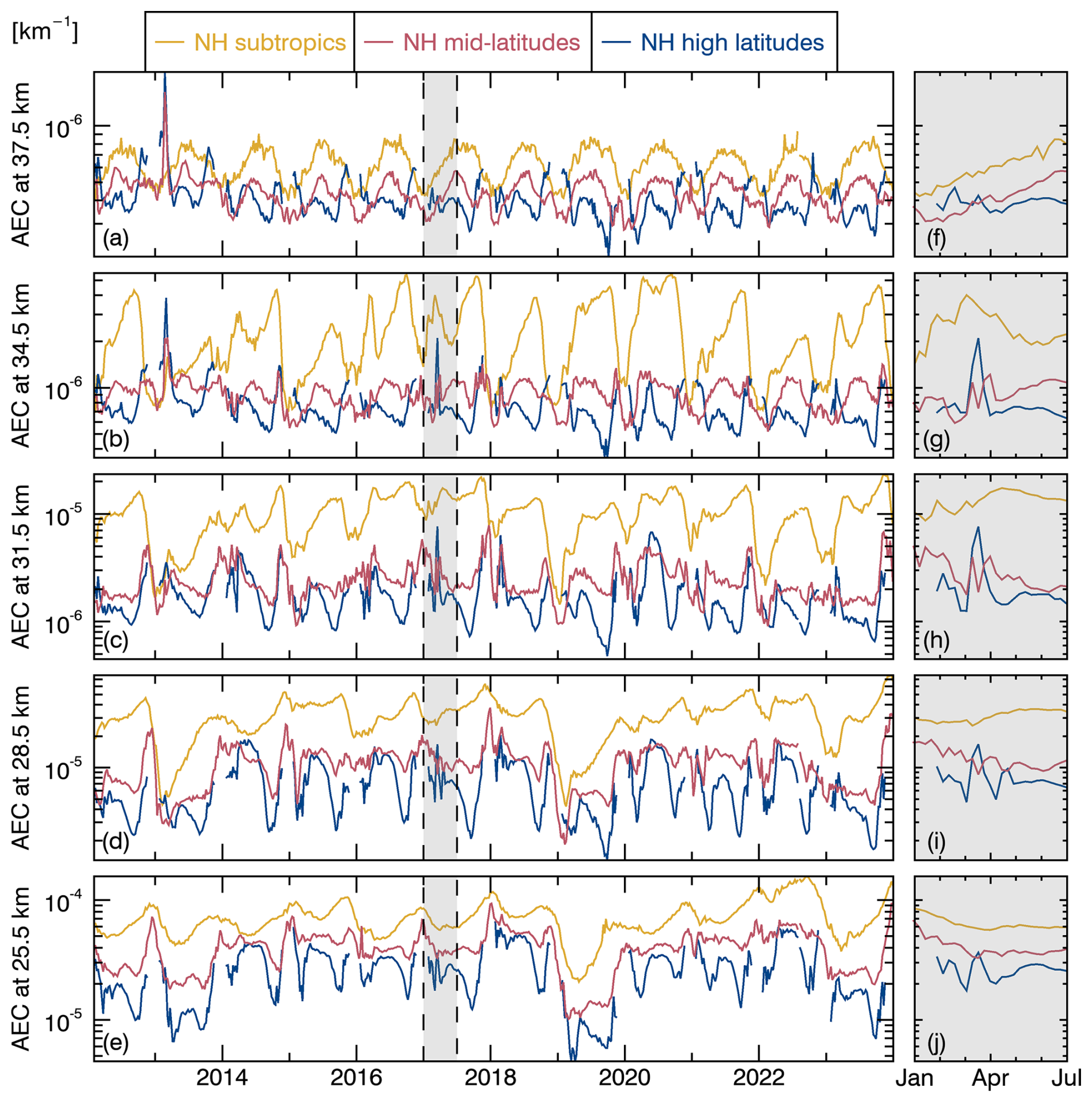
Figure 1 Weekly averaged aerosol extinction coefficient (AEC) at 869 nm from OMPS-UBr for five altitudes in the Northern Hemisphere (NH). The subtropics are defined from 20–40° N, the mid-latitudes from 40–60° N and the high latitudes from 60–80° N. The first half of 2017 is shaded within the dashed lines in (a–e) and zoomed in on the right-hand side in (f–j).

3 Results

3.1 Zonal mean aerosol extinction coefficient

Figure 1 shows the zonally averaged aerosol extinction coefficient (AEC) at 869 nm from OMPS-UBr in three distinct latitude ranges in the Northern Hemisphere at altitudes of 25.5, 28.5, 31.5, 34.5, and 37.5 km. During the OMPS period from 2012 to the present, there were several volcanic eruptions that had an impact on the stratosphere (e.g. Carn, 2025; Kovilakam et al., 2025). In the tropics, these were particularly the eruptions of Kelut (2014), Ambae (2018), Ulawun (2019), Soufriere St. Vincent (2021) and Hunga (2022). Moreover, two eruptions in mid-latitudes had an impact on the stratosphere. These were the eruptions of Calbuco in the Southern Hemisphere in 2015 and of Raikoke in the Northern Hemisphere in 2019. For the altitudes and latitude regions shown in Fig. 1, only a direct impact from the Hunga eruption is to be expected, whose plume was observed at an altitude of approximately 26 km (Duchamp et al., 2023). The impact of this eruption can be identified in Fig. 1e. After the eruption, the aerosol extinction coefficient reaches its maximum at an altitude of 25.5 km in the northern subtropics during the second half of 2022. The other eruptions referenced are not expected to exert a direct significant influence in the Northern Hemisphere at the altitudes shown.

In general, Fig. 1 shows a decrease in the aerosol extinction coefficient towards the pole. The meridional gradient and also the minimum extinction coefficient at high latitudes are most pronounced in late summer and early autumn. In addition, the aerosol extinction coefficient in the middle and high latitudes shows a stronger variance in the polar vortex season compared to the summer months. The occurrence of a local streamer event can be indicated by a jump in the weekly zonally averaged extinction coefficient at an altitude of 31.5 km, as observed in Fig. 1c.

In the northern high latitudes, indicated by the blue line in Fig. 1, a sudden increase can be observed in the mid-stratosphere in the weekly zonally averaged extinction coefficient in the shaded area in the first half of 2017. The signal is strongest at an altitude of 31.5 km. At this altitude, the aerosol extinction coefficient exhibited a sixfold increase in spring 2017, marking the highest value recorded at this altitude within the northern high latitudes during the OMPS measurement period. At altitudes of 28.5 and 34.5 km, the zonally averaged extinction coefficient increased by more than threefold. At an altitude of 28.5 km, the background level of the aerosol extinction coefficient is higher in other years than during early 2017 due to natural variations. At an altitude of 34.5 km, the peak in the extinction coefficient in 2017 is only exceeded by the signature of the Chelyabinsk meteor (Gorkavyi et al., 2013; Rieger et al., 2014), which exploded in the mid-stratosphere four years earlier in the spring of 2013. This is also the only period during the OMPS mission in which aerosol extinction is greater at middle and high latitudes than in the subtropics. An increase in the aerosol extinction coefficient in spring 2017 can also be observed, albeit to a lesser extent, at altitudes of 25.5 and 37.5 km.

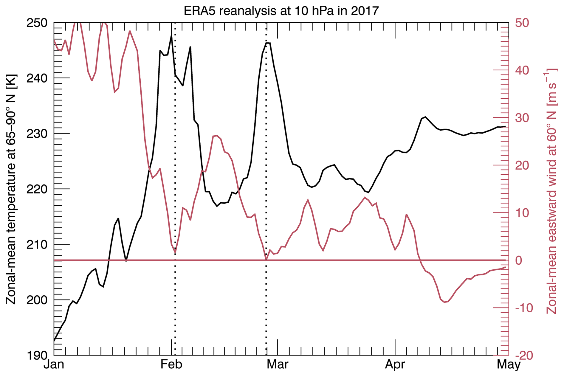
Figure 2 SSW criteria for spring 2017. The zonal mean eastward wind at 60° N is represented in red and the mean temperature from 65–90° N at 10 hPa is shown in black. Two minor SSWs in February are marked by dotted lines.

In the northern mid-latitudes, indicated by the red line in Fig. 1, two distinct peaks can be identified in March and April 2017 at altitudes of 28.5, 31.5, and 34.5 km, which are slightly less pronounced than in the high latitudes. At an altitude of 31.5 km, a more than twofold increase in the aerosol extinction coefficient is observed in these two peaks. The two peaks can be observed before and after the strongest increase in the high latitudes.

3.2 Aerosol extinction in the polar vortex season in early 2017

In Fig. 2, the zonal mean eastward wind at 60° N and and the temperature from 65–90° N at 10 hPa for early 2017 are shown. The representation is based on Baldwin et al. (2021). Two events, which are classified as minor warmings, are recorded at the beginning and end of February, which is consistent with the observations in Eswaraiah et al. (2019), Gogoi et al. (2023), and Li et al. (2023). A sudden increase in temperature can be observed at high latitudes. In addition, there is a weakening of the wind, but no reversal of the wind direction at 60° N and 10 hPa.

Figure 3 shows the development of the weekly averaged extinction coefficient interpolated to 10 hPa, i.e. approximately 30 km altitude for the initial 16 weeks of 2017. The figure shows the aerosol extinction coefficient at 869 nm in bins of 5° latitude and 15° longitude in the Northern Hemisphere.

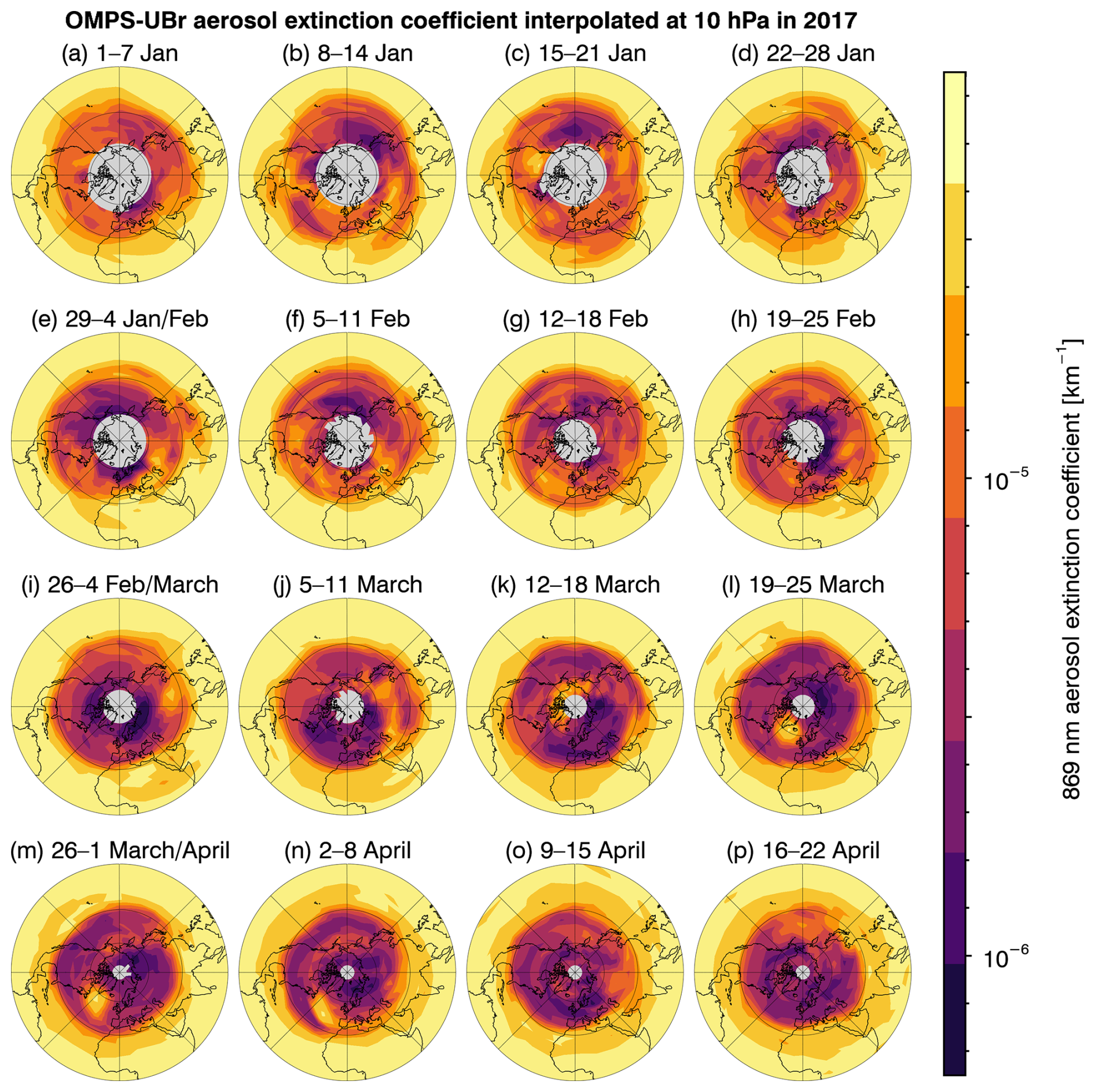
Figure 3 Polar stereographic maps of the weekly averaged aerosol extinction coefficient at 869 nm from OMPS-UBr interpolated to 10 hPa in early 2017 in bins of 5° latitude and 15° longitude for the entire Northern Hemisphere, with 0° E as the central longitude line from bottom to centre.

At the beginning of 2017, the aerosol extinction coefficient in the mid-latitudes is subject to considerable variation. Figure 3b and e show tongue-like patterns of increased aerosol extinction coefficient, extending from the subtropics to the mid-latitudes from west to central Asia. The increase in aerosol extinction that occurred subsequent to the second of these tongues in early February coincides with the first minor warming in 2017 (see Fig. 2), which caused a weakening and deflection of the vortex. At this time, the centre of the polar vortex was located at approximately 70° N. The increase in the aerosol extinction coefficient cannot be traced further in the following weeks.

On 25 February, a late minor SSW occurred (see Fig. 2). At a pressure level of 10 hPa, this had the effect of a temperature increase at the North Pole of more than 30 K. This phenomenon resulted in a weakening and separation of the polar vortex. A shift of the vortex edge into the subtropics can be observed from around 1 March. The vortex was subsequently elongated and displaced off the pole.

For a better understanding of the dynamic of the polar vortex, Fig. 4 presents in the lower five rows ERA5 reanalysis data for a four-week period in March and April 2017 following the second minor warming. The parameters under consideration are the wind, the potential vorticity with contour levels of geopotential height, the specific humidity, the ozone mass mixing ratio and the temperature, all at 10 hPa. The vortex centre itself is associated with low wind speed, geopotential height and ozone mixing ratio, and high potential vorticity and specific humidity. After the two minor SSWs, the polar vortex is no longer associated with low temperatures.

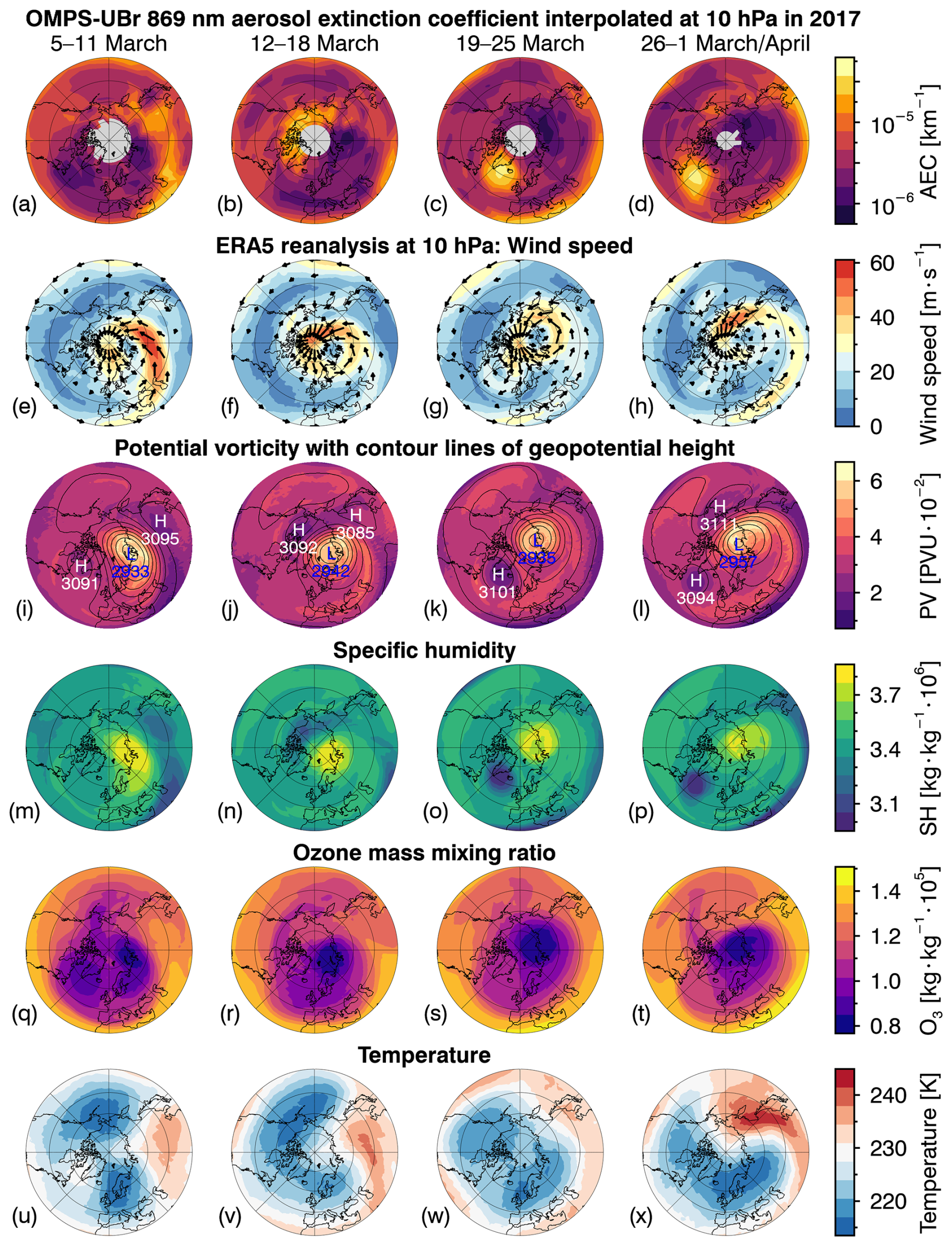
Figure 4 Polar stereographic maps from 30–90° N for weekly averaged parameters (rows) at 10 hPa for a period of 4 weeks in March and April 2017 (columns), indicated above the first row. First row contains the aerosol extinction coefficient at 869 nm from OMPS-UBr as in Fig. 3. Rows 2–6 show maps of ERA5 reanalysis data, including wind speed (e–h), potential vorticity in potential vorticity units and geopotential height in decametres (dam) (i–l), specific humidity (m–p), ozone mass mixing ratio (q–t) and temperature (u–x). Wind arrows are plotted at wind speeds of 10 m s⁻¹ or higher. The contour lines of the geopotential height are delineated at intervals of 0.2 km. The highest and lowest geopotential heights are denoted with “H” and “L”, respectively, along with the corresponding height in dam.

Looking at the first column of Fig. 4 for the week of 5–11 March, an increase in wind speed towards the pole of the now very uneven vortex can be observed. Following the displacement of the polar vortex towards the subtropics, the transportation of aerosols from the subtropics towards the pole can be deduced from the increased extinction coefficient at the edge of the vortex over Asia, see Fig. 4a and e. Subtropical air is transported along the edge of the polar vortex, and an area of high geopotential height or relative high pressure is formed, see Fig. 4i. An anticyclone forms around the area of high geopotential height. Areas of an increased aerosol extinction coefficient correlate with a low potential vorticity and the air parcel is dry and initially ozone-rich.

As of 16 March, the aerosols are observed to depart from the edge of the polar vortex. Concurrently, an anticyclone is established over Greenland (70° N, 45° W), see Fig. 4g and k. The aerosols are kept at the same longitude in the anticyclone for about three weeks, while slowly moving towards lower latitudes. Subsequently, from approximately 6 April onwards, the anticyclone can still be observed over the North Atlantic (45° N, 45° W). It is notable that the air parcel remains dry for the entire time that the signal is observable in the aerosol extinction coefficient. In the ozone mass mixing at this pressure level, the air parcel is no longer richer in ozone than the ambient air after a period of one week, at which point rapid mixing occurs. There is no evident correlation between increased aerosol extinction and temperature.

After 19 March, the formation of another streamer can be observed in a substantial area of low PV, low specific humidity and high ozone mass mixing ratio at 30° N over Asia. After 26 March, Fig. 4h, l, and p show the transport of this subtropical air to mid-latitudes. As can be seen in Fig. 4l, a further area of high geopotential height has formed over the Bering Sea.

Figure 5 shows a comparison of the vertical profiles of the aerosol extinction coefficient at middle to high latitudes, both inside and outside the anticyclone, and in the tropics over central and northern Africa at the beginning of March before the start of the streamer event. To make this comparison, profiles from the same geographical region (55–70° N and 20–45° W) were averaged for different weeks before and during the streamer event, as in Fig. 3j and l. To compare these with the vertical profile of the aerosol extinction coefficient from the region in which the streamer likely originated, measurements before the start of the streamer event (see Fig. 3i) from the tropics to subtropics (0–30° N, 0–45° E) were averaged.

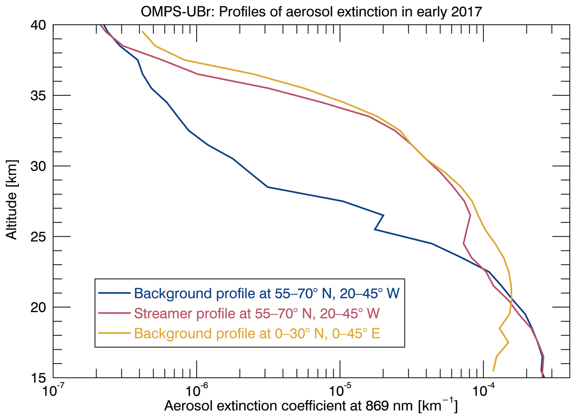
Figure 5 Weekly averaged profiles of the aerosol extinction coefficient in middle to high latitude (55–70° N, 20–45° W) for background conditions before the streamer event (5–11 March) and inside the anticyclone during the streamer event (19–25 March), and in the tropics to subtropics (0–30° N, 0–45° E) before the start of the streamer event (26 February–4 March).

At an altitude of 26–38 km the vertical profiles in the tropics and three weeks later in the anticyclone differ only slightly. This suggests that there was little mixing of aerosols with the ambient air along the transport path. The high-pressure area, which transports tropical air towards higher latitudes, creates a barrier for mixing between the anticyclone and the surrounding air. The agreement between the profiles inside the anticyclone and from the subtropics is greatest at 30.5 km, the altitude at which the strongest signal from the streamer, i.e. the biggest percentage increase in the aerosol extinction coefficient, is visible. Up to an altitude of around 26 km, there is a clear distinction in the profiles of subtropical and high-latitude regions. Conversely, a high degree of similarity is observed between the profiles both within and outside the anticyclone up to this altitude. At an altitude of 32.5 km, the aerosol extinction coefficient increases by a factor of 27 from the background level to the streamer. In addition to 2017, anticyclones in the mid-latitudes are also evident in the aerosol extinction coefficient in other years, e.g. 2015 and 2022, albeit to a lesser extent (not shown).

As of 13 March, a weak polar vortex streamer becomes discernible in the reanalysis data, see the second column of Fig. 4. This is evident below 45° N over Southern Europe in an increased potential vorticity, see Fig. 4j, an increased specific humidity, see Fig. 4n, and also a reduced aerosol extinction coefficient, see Fig. 4b.

3.3 Estimation of the transported aerosol mass in 2017

For the estimation of the transported aerosol mass, it is important to note that measurements with SAGE III on ISS began in June 2017, precluding the possibility of direct overlap with the observed signatures in 2017 and earlier. Consequently, the PSD parameters for comparable atmospheric conditions in subsequent years must be used. To this end, a streamer event from 2018 was selected. It began in February 2018, a few weeks earlier in the season than in 2017, and was observable with SAGE III/ISS in early March. Below 31 km altitude, the streamer had a comparable zonal influence on the aerosol extinction coefficient as in 2017 and was also briefly located in the high latitudes, see Fig. 1. Since there was no volcanic eruption between the two events in 2017 and 2018 that could have affected the stratosphere, the background aerosol level remained consistent. The present study focuses on the streamer event in early 2017 due to its greater vertical extent, its stronger influence on high latitudes, and the fact that there was negligible mixing taking place due to the anticyclone.

Figure 6 shows vertical profiles of the two streamers in 2017 and 2018 in the mid-latitudes (45–55° N) for different longitude regions as measured with OMPS-LP and SAGE III/ISS. Both streamer profiles originate from a time approximately 3–4 weeks after the start of the streamer event. Up to an altitude of 34 km, there is very good agreement between the retrieved aerosol extinction coefficient with OMPS-UBr and SAGE III/ISS in 2018. This indicates that the streamer event in 2018 can be observed with both instruments. The vertical profile from 2017 shows a higher average aerosol extinction over the entire altitude range of the streamer. This can be partially explained by the fact that the streamer in 2017 is more compressed within an anticyclone, thereby concentrating the aerosols in a smaller area.

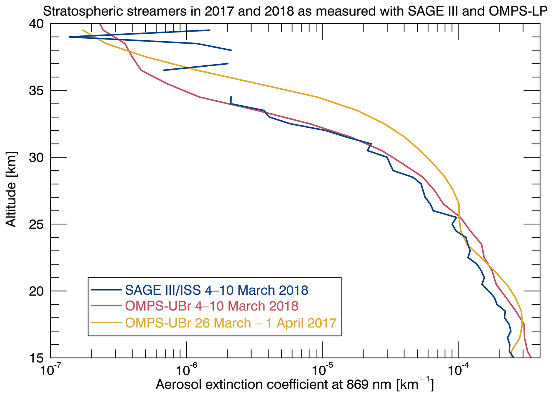
Figure 6 Mean vertical profiles of aerosol extinction at 869 nm for two streamers in mid-latitudes from 26 March to 1 April 2017 (45–55° N, 25–50° W) and from 4–10 March 2018 (45–55° N, 10° W to 15° E) as retrieved from OMPS-LP and SAGE III/ISS measurements.

Nevertheless, this period in March 2018 and this region appears to be the best possible match with the streamer event in 2017 in the measurement period of SAGE III. For this selection, the mean median radius and geometric standard deviation of a monomodal log-normal distribution are obtained for every altitude step. The Mie code of the University of Oxford is used to calculate the extinction cross section for these PSD parameters.

The time period spanning 14 d from 19 March to 1 April is selected for the estimation of the transported sulfate aerosol mass in spring 2017. This is due to the aerosol layer exhibiting minimal zonal or meridional movement during this interval, thereby facilitating its observation over the North Atlantic. The mean extinction coefficient at 869 nm is calculated for each height level from 24.5–38.5 km for grid boxes of size 3°×3°. Furthermore, the mean extinction coefficient from 0–270° E, i.e. in the range in which no increase in the aerosol extinction coefficient due to transported material can be observed, is calculated for each latitude step. Grid boxes are designated as an anomaly if the extinction coefficient is higher than its latitudinal mean plus three times the standard deviation and if an increase is also observed in the surrounding grid boxes.

For each such anomaly, the absolute number of particles N(z) at height z is calculated. The height z is defined as the centre height of an altitude layer spanning 1 km. The volume V of the respective grid box and the number density N₀(z) are used to calculate the absolute number of particles N(z). The number density is derived from the additional aerosol extinction attributable to the streamer and the PSD parameters. The mass of a log-normally distributed aerosol population can then be calculated using the 3rd moment of the log-normal distribution (Seinfeld and Pandis, 2016).

$$\begin{array}{}\text{(1)}& {\displaystyle }{\displaystyle }m\left(z\right)={\displaystyle \frac{\mathrm{4}}{\mathrm{3}}}\mathit{\pi }\cdot N\left(z\right)\cdot r_{\text{med}}^{\mathrm{3}}\cdot \mathit{\rho }(z,T)\cdot \exp \left({\displaystyle \frac{\mathrm{9}}{\mathrm{2}}}\ln ({\mathit{\sigma }}_g{)}^{\mathrm{2}}\right)\end{array}$$

In this equation, m(z) denotes the total mass of the aerosol population at height z and ρ(T) represents the density of the aerosol particles as a function of temperature T at height z. For the mass density ρ, the measured mass densities of sulfuric acid for different mass fractions and temperatures of Myhre et al. (1998) are interpolated for an H₂SO₄ mass fraction of 75 % and for the respective GMAO temperature at this altitude.

The aerosol mass that has been transported in 2017, as calculated with averaged PSD parameters for measurements of the streamer event in 2018, is estimated to be approximately 0.99 kt in the altitude range of 24.5–38.5 km, where the aerosol extinction signal of this air parcel is observable.

Since the aerosol extinction coefficient changes only slightly along the transport path of the streamer, see Fig. 5, it is assumed that changes in mass along the path are also negligible. For the high latitudes defined as 60–90° N, the average PSD parameters from SAGE III/ISS for the same altitude range result in a total mass of 1.34 kt for background conditions. This means that the streamer event in the week of 12–18 March causes a zonal increase in the total aerosol mass in the altitude range of 24.5–38.5 km by about 74 %. At an altitude of 30.5 km, the aerosol mass in the high latitudes zonally increases by about 260 % during the same period. On a local scale, the mass can increase by more than one order of magnitude.

3.4 Aerosol extinction in the polar vortex season in early 2005

Manney et al. (2006) observed a strong and long-lasting FrIAC in 2005. This subsection will examine whether this can also be observed in the aerosol extinction coefficient. A notable peak in the aerosol extinction coefficient in the mid-stratosphere during the SCIAMACHY measurement period was observed in spring 2005. Figure 7 shows the aerosol extinction coefficient at 750 nm in the Northern Hemisphere interpolated at an altitude of 30.5 km from spring to late-summer 2005. The northern winter of 2004/05 was relatively cold with prolonged periods of temperatures below 200 K in the lower stratosphere and characterized by a strong and stable polar vortex (e.g. Sonkaew et al., 2013). On 13 March, there was an exceptionally early final warming, approximately one month before the historical median (Butler and Domeisen, 2021). As can be seen in Fig. 7a–d, there are some variations in March 2005 in the mid-latitudes. From the end of March/beginning of April an increase in the aerosol extinction coefficient at the pole is noticeable.

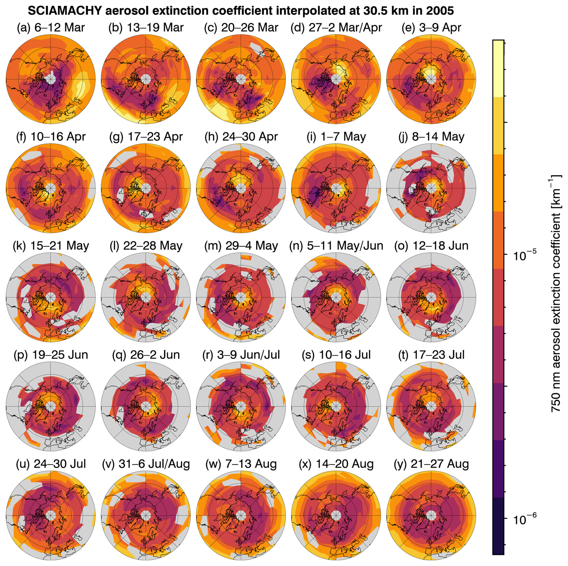
Figure 7 Polar stereographic maps of the weekly averaged aerosol extinction coefficient at 750 nm from SCIAMACHY interpolated at 30.5 km in from March to August 2005 in bins of 5° latitude and 15° longitude from 30–90° N.

Figure 8 presents in the lower five rows reanalysis data for the four weeks from March to early April. Before the final warming on 13 March, a slightly increased aerosol extinction coefficient can already be observed in the mid-latitudes across a substantial geographical area extending from North America to the Pacific region, see Fig. 8a. This suggests that subtropical air has already accumulated in a high-pressure area extending over a considerable region, see Fig. 8i. In the weeks following the final warming, the region of low geopotential height of the collapsed polar vortex shifts towards mid-latitudes, see Fig. 8j. Concurrently, the low-pressure area is compressed and shifts towards the pole until the end of March. By then, a strengthening anticyclone develops with low PV (Fig. 8l), dry ozone-rich air (Fig. 8p and t) and high aerosol extinction (Fig. 8d) over the Arctic Ocean near Siberia. The anticyclone shifts towards the pole and remains there trapped in the circulation for a period of several months until August of the same year, see Fig. 7. Similar structures to those seen in 2005 can be found in other years in the aerosol data sets examined, e.g. in 2006, 2007, and 2014 (not shown).

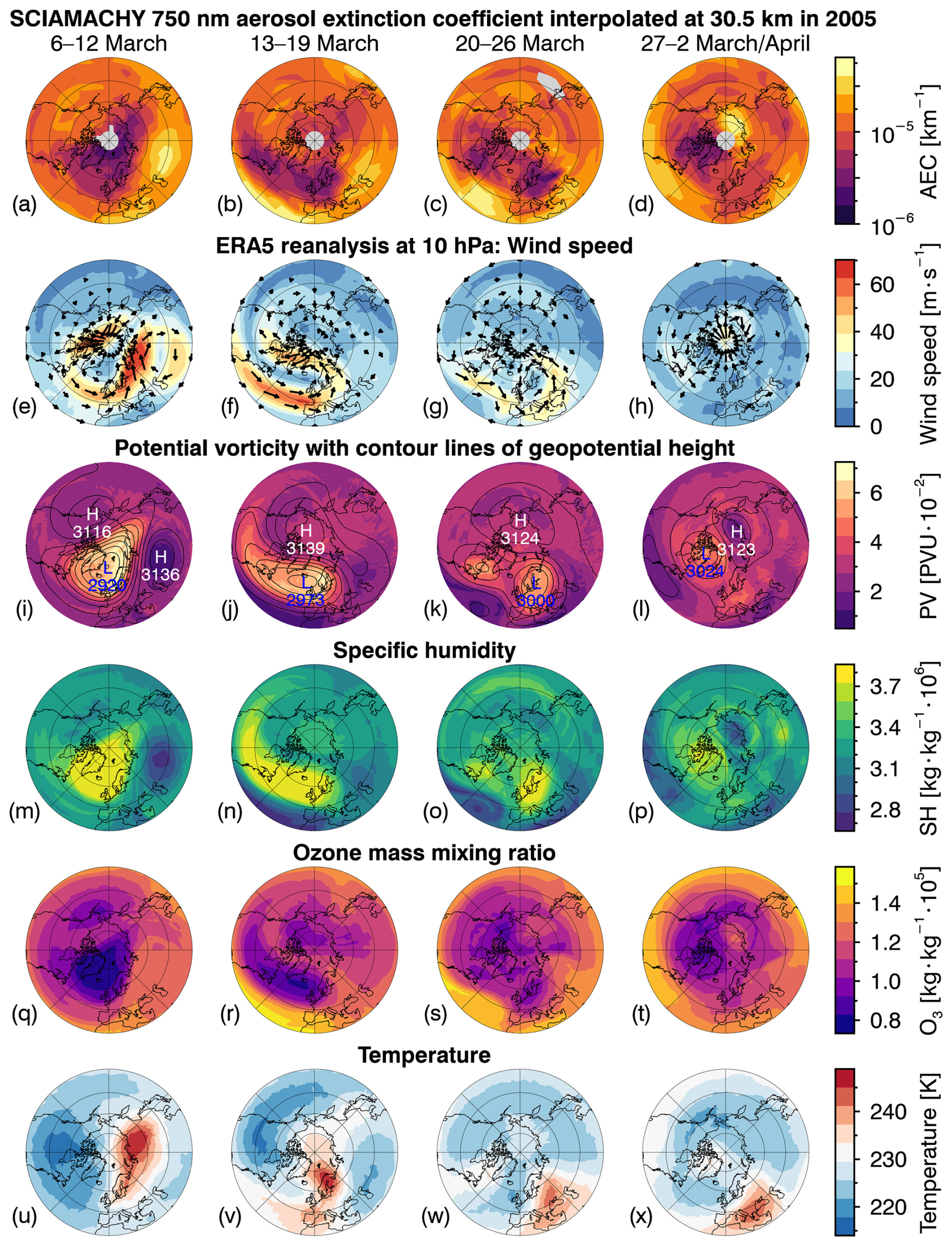
Figure 8 Polar stereographic maps from 30–90° N for weekly averaged parameters (rows) for a period of 4 weeks in March and April 2005 (columns), indicated above the first row. First row contains the aerosol extinction coefficient at 750 nm from SCIAMACHY as in Fig. 7 at an altitude of 30.5 km. Rows 2–6 show maps of ERA5 reanalysis data at 10 hPa, including wind speed (e–h), potential vorticity in potential vorticity units and geopotential height in dam (i–l), specific humidity (m–p), ozone mass mixing ratio (q–t) and temperature (u–x). Wind arrows are plotted at wind speeds of 10 m s⁻¹ or higher. The contour lines of the geopotential height are delineated at intervals of 0.2 km. The highest and lowest geopotential heights are denoted with “H” and “L”, respectively, along with the corresponding height in dam.

4 Sources of error

It is conceivable that the observed signal is an artefact of the retrieval product or a specific measurement technique. However, the transport in 2017 can be observed in a very similar way in the other OMPS-LP retrieval products from NASA and the University of Saskatchewan. The FrIAC in 2005 can also be observed using aerosol extinction data collected by SCIAMACHY. This suggests that the observed phenomena are not artefacts of a single retrieval or instrument. However, both phenomena are detected using a similar measurement technique. For comparison with the aerosol extinction coefficient from a solar occultation instrument, a streamer event from 2018 was selected, which could be observed by both SAGE III/ISS and OMPS-LP, see Fig. 6.

Up to an altitude of 34 km, there is very good agreement between the two profiles of the different satellite instruments. The observation of increased aerosol extinction profiles up into the mid-stratosphere at mid-latitudes using two instruments with different measurement techniques and retrieval methods, indicates that this is a genuine aerosol extinction signal.

The likelihood of an error in retrieval due the effects of water vapour and ozone during the streamer event is negligible, as the two trace gases exhibit only very low absorption at the wavelength channels used. Increased ozone levels at an altitude of 30 km and above can only be observed during the first week of the streamer's presence. Additionally, the streamer is drier than the surrounding air.

The estimated amount of just below 1 kt depends heavily on the number density of the aerosols, which in turn depends on the assumptions made about the size distribution, i.e. the median radius and geometric standard deviation. For this estimation, the ”weighted median PSD parameters” from the SAGE III/ISS dataset (Knepp et al., 2024) were employed for every altitude step when a streamer in 2018 was measured in mid-latitudes with SAGE III/ISS.

This is a very rough estimate. Therefore, the assumptions about the PSD parameters were varied. To vary the PSD parameters, a single averaged PSD combination from the altitude range of 25–30 km was applied to the entire altitude range. This is owing to the fact that PSD retrieval is more reliable at lower altitudes than at high altitudes. In addition, PSD parameters from 0–30° N from the entire SAGE III/ISS measurement period up to the Hunga eruption were averaged for each altitude step. However, both methods result only in a negligible deviation of about 5 % in aerosol mass.

Nevertheless, the estimate remains uncertain. No solar occultation measurements are available for spring 2017. The true PSD of aerosols above 30 km altitude is largely unknown and is subject to high bias and error when retrieved from SAGE measurements. In addition, there is general uncertainty about the true shape of the size distribution, which is assumed to be monomodal for the retrieval. However, if the true shape is different, e.g. bimodal, this can lead to significant deviations in the retrieval of PSD parameters (von Savigny and Hoffmann, 2020).

5 Discussion

Both described events in 2005 and 2017 can be explained by the combination of streamers, transporting tropical air into the middle or high latitudes and anticyclones holding material in these regions. The exact extent and shape of the polar vortex and how far it reaches into the mid-latitudes appears to be decisive for the transport of aerosols towards the pole. In the majority of years in the observation period 2003–2023, a transport of tropical air into the mid-latitudes and a variation in the aerosol extinction especially in mid-latitudes can be observed. The intensity depends largely on the background level in tropical aerosol extinction. The duration and stability of a streamer depend on the dynamics in mid-latitudes in connection with the polar vortex and whether the streamer is associated with an anticyclone, which, as in 2017, prevents mixing with the surrounding air.

During early 2017, two minor warmings occurred in February 2017. The impact of the former on the mesosphere was described in Eswaraiah et al. (2020). A streamer event can also be observed in the stratospheric aerosol extinction coefficient following this first warming at the beginning of February, during which tropical air is transported to mid-latitudes. However, this signal is only observable for approximately one week, and the high latitudes are not adequately covered by OMPS-LP at the beginning of February. Consequently, the estimation of transport was only possible via surrounding latitudes on the outward or return transport from the pole. The reanalysis data indicates that no anticyclone is formed, thereby ensuring that the transported air parcel of the streamer does not remain concentrated at middle and high latitudes. Moreover, the signal in the specific humidity is no longer clearly observable after one week.

A notable characteristic of the polar vortex season 2017 is the comparatively late occurrence of a warming, i.e. the second minor warming, which was not also the final warming in the vortex season (Gogoi et al., 2023). This phenomenon enables the observation of the signal of an increased extinction coefficient above 75° N. The sequence of weakening, deflection and brief but repeated strengthening of the elongated vortex with high wind speeds in the direction of the pole and low speeds away from the pole ensures that aerosols can accumulate at the pole. The vortex weakens once more, causing the material to remain in the mid-latitudes for several weeks. The formation of a high-pressure system, accompanied by the establishment of an anticyclone, results in the accumulation of material south of Greenland over the Atlantic.

Following the second warming, no correlation of low temperatures with the vortex or high temperatures with the streamer is discernible in the temperature profile. This exemplifies the significant weakening of the polar vortex, which did not regain its closed circular structure and strength following the two minor SSWs. In addition, the temperature gradient between the tropics and high latitudes is only marginal, which is why the transported air mass is no longer associated with increased temperatures.

Tropical-subtropical streamers can occur at any time of the year, although streamer frequency is significantly higher during the polar vortex season (Offermann et al., 1999; Eyring et al., 2003). However, the coverage of the high latitudes by the limb instruments used decreases towards the end of the year, making it more difficult to track the course of a streamer.

It is important to note that, in contrast to the more prevalent occurrence of streamer events in the Northern Hemisphere, these events are less frequent in the Southern Hemisphere due to the presence of a more stable vortex (van Loon et al., 1973). The more-frequent observation of this phenomenon in the Northern Hemisphere may also be explained, by the elevated background level of the aerosol extinction coefficient in the mid-stratosphere in the southern mid-to-high latitudes. This results in a lower gradient of the aerosol extinction coefficient between the South pole and the tropics compared to the gradient between the North pole and the tropics. Consequently, the presence of streamer events in the Southern Hemisphere is less pronounced in the aerosol extinction coefficient. However, this observed difference in the gradient may also result from increased retrieval uncertainties in the Southern Hemisphere (Chen et al., 2020). The scattering angles of aerosols are strongly dependent on latitude for OMPS-LP measurements and change during the orbit. The observed signal in the Southern Hemisphere originates, among other things, from aerosol scattering in the sideways and backward directions, while in the Northern Hemisphere, forward scattering predominates.

The observed signal in 2017 shows good agreement with the characteristics expected from runs for stratospheric streamers with the Freie Universität Berlin Climate Middle Atmosphere Model (FUB-CMAM) in Krüger et al. (2005). These also showed a higher probability of streamers occurring when the polar vortex shifted equatorward. The dimensions of the streamer in 2017, with a length of over 10 000 km in the development phase, a width of about 1500 km and a vertical extent of about 14 km, correspond very well with the modelled extent of streamers. The duration of the event, spanning five weeks, is at the upper end of the expected time frame. This can be attributed to the anticyclone in 2017, which kept the tropical air in mid-latitudes for an extended period of time. The observation made in 2017 of a transport to 70–75° N also occurs in the model used in Krüger et al. (2005) in some years. In contrast to the model, no evidence of irreversible mixing at high latitudes is observed in 2017. The streamer in 2017 is located over East Asia, where the model predicts the maximum number of streamer events.

It is possible to observe different tracers of streamers and anticyclones for varying lengths of time. Ozone mixing, for instance, is a highly potent process that occurs in March 2017 a few days after the start of the streamer event. This mixing occurs more rapidly at higher altitudes (10 hPa, ∼31 km) than at lower altitudes (20–30 hPa, ∼23–26 km). At these lower altitudes, the air mass is still rich in O₃ even at the end of March. This observation is consistent with Thiéblemont et al. (2011), who also demonstrated in their description of a FrIAC in 2007 that the ozone mixing ratio decreases much faster at 10 hPa than at 20 hPa. The ozone signal is more strongly linked to gas chemistry and photochemistry than to mixing processes. The process of relaxation to lower ozone levels is even faster in spring, due to higher levels of solar radiation (Manney et al., 2006). Conversely, elevated aerosol levels and diminished levels of specific humidity persist within the anticyclone for a period of approximately one month. The correlation of anticyclone and dry air in the specific humidity is observable up to higher altitudes (5–20 hPa, ∼26–35 km).

The FrIAC in 2005 has already been described in detail based on observations (Manney et al., 2006) and modelling (Allen et al., 2011). As in Manney et al. (2006) for the trace gases N₂O and H₂O, the signature of the FrIAC can be observed in the extinction coefficient until August. Similar to 2005, FrIACs of varying intensity can also be seen in the Northern Hemisphere in 2006, 2007, and 2014 (not shown), subsequent to the breakdown of the polar vortex. These circumpolar areas can be identified by a slight increase in the extinction coefficient at high latitudes.

6 Conclusions

We have described a stratospheric tropical-subtropical streamer and a frozen-in anticyclone that can be observed in an increased aerosol extinction coefficient in two case studies in 2017 and 2005. Streamers are horizontal transport processes by which atmospheric trace substances can be transported over long distances. Anticyclones can hold low latitude air in middle or high latitudes for periods ranging from weeks to several months. The signatures of these events were compared with ERA5 meteorological reanalysis data. While ozone mixes rapidly in both the streamer and the FrIAC, these two phenomena are evident in the aerosol extinction coefficient for as long as they are present in specific humidity.

Streamers are generally associated with disturbances in the polar vortex and a deflection of the vortex towards the subtropics. The streamer event of 2017 could be observed after a comparatively late second minor SSW in the polar vortex season. This allowed tropical air to cross the subtropical transport barrier. FrIACs can occur both during the polar vortex season, such as in 2017 when the transported tropical air mass was held over the North Atlantic for several weeks, or after the polar vortex breakdown, as was the case in 2005. In 2005, a FrIAC was observed in an increased aerosol extinction coefficient in the high latitudes from March to August.

The amount of sulfuric acid aerosols transported in the streamer towards middle and high latitudes in early 2017 was estimated to be approximately 1 kt, using aerosol properties derived from SAGE III/ISS PSD data for a comparable streamer event in 2018. A variation in the selected size parameters results in only a slight change in aerosol mass of about 5 %. The 2017 event was the most significant poleward aerosol transport by streamers observed in the last twenty years. It almost doubled the aerosol mass in high latitudes for the altitude range of 24.5–38.5 km of the streamer. On a local scale, the aerosol extinction coefficient increased by a factor of 27.

The transport of tropical aerosol-rich air to mid-latitudes is not an uncommon phenomenon and occurs to a small extent multiple times every year. However, the observation of a tropical-subtropical streamer reaching high latitudes is a rare occurrence. In 2017, this is even evident in the zonal mean aerosol extinction at high latitudes. The correlation between streamer events and aerosol extinction coefficients was demonstrated for the first time in this study. This correlation as well as the connection between streamers and anticyclones in 2017 provide new insights into the poleward transport and persistence of tropical air in the middle stratosphere at the end of the polar vortex season.