Quantifying European SF₆ emissions from 2005 to 2021 using a large inversion ensemble

Sulfur hexafluoride (SF₆) is a highly potent and long-lived greenhouse gas whose atmospheric concentrations are increasing due to human emissions. In this study, we determine European SF₆ emissions from 2005 to 2021 using a large ensemble of atmospheric inversions. To assess uncertainty, we systematically vary key inversion parameters across 986 sensitivity tests and apply a Monte Carlo approach to randomly combine these parameters in 1003 additional inversions. Our analysis focuses on high-emitting countries with robust observational coverage – UK, Germany, France, and Italy – while also examining aggregated EU-27 emissions.

SF₆ emissions declined across all studied regions except Italy, largely attributed to EU F-gas regulations (2006, 2014), however, national reports underestimated emissions: (i) UK emissions dropped from 68 (47–77) t yr⁻¹ in 2008 to 19 (15–26) t yr⁻¹ in 2018, aligning with the reports from 2018 onward; (ii) French emissions fell from 78 (51–117) t yr⁻¹ (2005) to 35 (19–54) t yr⁻¹ (2021), exceeding reports by 88 %; (iii) Italian emissions fluctuated (25–48 t yr⁻¹), surpassing reports by 107 %; (iv) German emissions declined from 182 (155–251) t yr⁻¹ (2005) to 97 (88–104) t yr⁻¹ (2021), aligning reasonably well with reports; (v) EU-27 emissions decreased from 403 (335–501) t yr⁻¹ (2005) to 225 (191–260) t yr⁻¹ (2021), exceeding reports by 20 %. A substantial drop from 2017 to 2018 mirrored the trend in southern Germany, suggesting regional actions were taken as the 2014 EU regulation took effect.

Our sensitivity tests highlight the crucial role of dense monitoring networks in improving inversion reliability. The UK system expansions (2012, 2014) significantly enhanced result robustness, demonstrating the importance of comprehensive observational networks in refining emission estimates.

1 Introduction

Sulfur hexafluoride (SF₆) is a fluorinated gas (F-gas), which has the highest global warming potential (GWP) of all known greenhouse gases (GHG), with current estimates of 18 400, 24 700, and 29 800 for 20, 100, and 500-year time horizons, respectively (WMO, 2022). Even more concerning, estimates of its atmospheric lifetime range between 850 and 1280 years (WMO, 2022), implying that SF₆ from past, present, and future anthropogenic emissions will accumulate in the atmosphere and will warm the climate for thousands of years.

Since the late 1990s, global SF₆ mole fractions have almost tripled, from 4.2 ppt in 1998 to 11.4 ppt in 2023 (Lan et al., 2024b), while global atmospheric growth rates have more than doubled, from 0.20 t yr⁻¹ in 1998 to 0.41 t yr⁻¹ in 2023 (Lan et al., 2024b). Radiative forcing increased from 2.4 in 1998 to 6.2 mW m⁻² in 2022. If the current global emission trend continues, SF₆ radiative forcing could increase up to 70 mW m⁻² by the end of the century (Hu et al., 2023).

Due to its high stability, SF₆ is used mainly as an insulator for electric equipment in the power industry (e.g. IEEE, 2012; Koch et al., 2018; Cui et al., 2024), with emissions occurring during equipment leakage, failures, maintenance, and decommissioning. It is also used in the metal industry as a blanketing gas (e.g. Maiss and Brenninkmeijer, 1998), as a cover gas in magnesium production and processing (Bartos et al., 2007; Ottinger et al., 2015), for semiconductor manufacturing for equipment cleaning and plasma etching (e.g. Cheng et al., 2013), and in the past it was even used to fill sports shoes (Pedersen, 2000) and car tires (Schwaab, 2000). In the 1990s, especially in Western Europe, SF₆ was used to fill double-glazed windows (e.g. Schwarz, 2005), which still represents a substantial European emission source (United Nations Framework Convention on Climate Change, 2023).

SF₆ was regulated under the Kyoto Protocol, where it is listed as one of the six categories of major GHGs (United Nations Framework Convention on Climate Change, 1997). To meet the Kyoto Protocol's targets, the EU passed regulation No. 842/2006 (EU, 2006), setting rules for the containment, recovery, use, and reporting of fluorinated gases. It banned the use of SF₆ in vehicle tires (starting in 2007) and in large-scale magnesium die-casting (starting in 2008), as well as in soundproof windows and footwear. The EU's 2014 regulation (No.517/2014, EU, 2014) further restricted SF₆ use, requiring leak detection systems for electrical switchgear by 2017 and banning it from recycling magnesium alloys by 2018. The new 2024 F-gas regulation mandates the phase-out of F-gases in medium-voltage switchgear by 2030, high-voltage switchgear by 2032, and prohibits SF₆ use for switchgear maintenance by 2035, unless reclaimed or recycled (EU, 2024).

A key aspect of the Kyoto Protocol was the implementation of a robust system for monitoring GHG emissions, requiring Annex-I countries (industrialized countries) to submit annual reports to the United Nations Framework Convention on Climate Change (UNFCCC), including SF₆. These reports are almost exclusively calculated by so-called bottom-up methods, where statistical data on economic production and consumption are combined with source-specific emission factors to estimate national emissions. The Emissions Database for Global Atmospheric Research (EDGAR) and the Greenhouse Gas and Air Pollution Interactions and Synergies (GAINS) model also provide bottom-up inventories of SF₆ emissions. However, due to inherent uncertainties associated with bottom-up methods, there is a strong demand for independent verification (e.g. Weiss et al., 2021), which can be achieved through top-down approaches, such as inverse modeling (e.g. Leip et al., 2017). In an inversion approach, atmospheric observations are used together with an atmospheric transport model to optimize the emissions.

Several inversion studies have investigated SF₆ emissions, however, limited research has specifically focused on the European continent. The global inversion study by Rigby et al. (2010) estimated total European SF₆ emissions from 2004 to 2008, distinguishing between emissions from reporting and non-reporting countries. Ganesan et al. (2014) estimated SF₆ emissions for 2012 in well-monitored countries, including Germany, France, and the UK. Their estimates indicated higher emissions than those officially reported to the UNFCCC. Brunner et al. (2017) used four independent inverse models to estimate European SF₆ emissions in 2011. Their results were 47 % higher than the UNFCCC reports, with Germany identified as the largest emitter. Simmonds et al. (2020) used three different inversion systems to estimate total SF₆ emissions from western Europe between 2013 and 2018, with one of the systems extending its analysis to cover 2007–2018. Their calculated emissions ranged from comparable to significantly higher than the reported values. Their work also suggested substantial SF₆ emissions in southwest Germany. In the UK's annual report to the UNFCCC, Manning et al. (2022) presented inversion results for SF₆ emissions in both the UK and northwest Europe, revealing a downward trend in both regions. The global inversion study by Vojta et al. (2024) provided an annual SF₆ time series for the aggregated EU-27 emissions, between 2005 and 2021. They found a decline in SF₆ emissions, with a significant drop in 2018, which they attributed to the impact of the EU's 2014 F-gas regulation.

While recent studies have employed regional high-resolution inversions to constrain SF₆ emissions in China (An et al., 2024) and the U.S. (Hu et al., 2023), there is no recent high-resolution regional study examining the trend of SF₆ emissions in Europe. This research endeavors to bridge a significant gap in our understanding of European SF₆ emissions. We adopt the methodology established by Vojta et al. (2024), adapting it for a high resolution (0.25×0.25°) inversion covering all of Europe. Utilizing the same datasets, we quantify SF₆ emissions across the continent for the period 2005 to 2021. While Vojta et al. (2024) primarily investigated the influence of different a priori inventories, this study delves deeper by conducting a comprehensive sensitivity and uncertainty analysis. We systematically examine the impact of a wide range of parameters on our inversion results, enabling a more robust quantification of overall uncertainties and a thorough investigation of the sensitivity to individual inversion components.

2 Methods

2.1 Measurement data

In this study, we utilize the same global observational dataset as employed by Vojta et al. (2024), where a detailed description is available. Therefore, we only provide a brief overview here. The dataset is based on globally distributed atmospheric observations of SF₆ dry-air mole fractions collected between 2005 and 2021. It includes continuous on-line measurements, instantaneous flask sample data from surface stations, and observations from mobile platforms. The measurements were contributed by various independent organizations such as the National Oceanic and Atmospheric Administration (NOAA) and the Advanced Global Atmospheric Gases Experiment (AGAGE) international network. Continuous surface measurements were averaged over 3 h intervals and all observations were standardized to the SIO-2005 calibration scale (for more details see Vojta et al., 2024). It is noteworthy that the number of available European on-line monitoring stations increased over the study period. While at the beginning only 5 such stations were available (Bialystok: BIK, Jungfraujoch: JFJ, Mace Head: MHD, Zeppelin: ZEP, Zugspitze-Schneefernerhaus: ZSF), the monitoring network in Western Europe significantly expanded with the addition of UK observations from Ridge Hill (RGL) and Tacolneston Tall Tower (TAC) in 2012 and further from Bilsdale (BSD) and Heathfield (HFD) in 2014. Figure S1 in the Supplement provides an overview of all the ground-based measurements globally, while Fig. 1 shows the stations in Europe.

To determine the influence of data selection criteria on our results, we created eight different subsets. (1) We used the entire global dataset (presented in Vojta et al., 2024), and (2) we created a European subset by excluding on-line stations outside Europe (BRW, CGO, COI, GSN, HAT, IZO, MLO, NWR, RPB, SMO, SPO, SUM, THD; see Fig. S1) while retaining the European sites¹ (BIK, BRM, BSD, CMN, HFD, JFJ, MHD, RGL, TAC, ZEP, and ZSF; see Fig. 1). Note that the stations SUM in Greenland and IZO in Tenerife are geographically closest to the European inversion domain. For these global and European datasets, we further refined the selection by: (a) retaining only night observations (00:00–06:00) at mountain stations and afternoon observations (12:00–18:00) at all other sites for continuous monitoring stations; (b) creating a data subset that excludes mountain stations, and (c) generating a subset that omits low-frequency measurements and data from moving platforms, retaining only high-frequency surface observations. Table S1 in the Supplement provides the number of observations used from each dataset for each year, whereas Table S2 shows the availability of online measurements within and outside Europe.

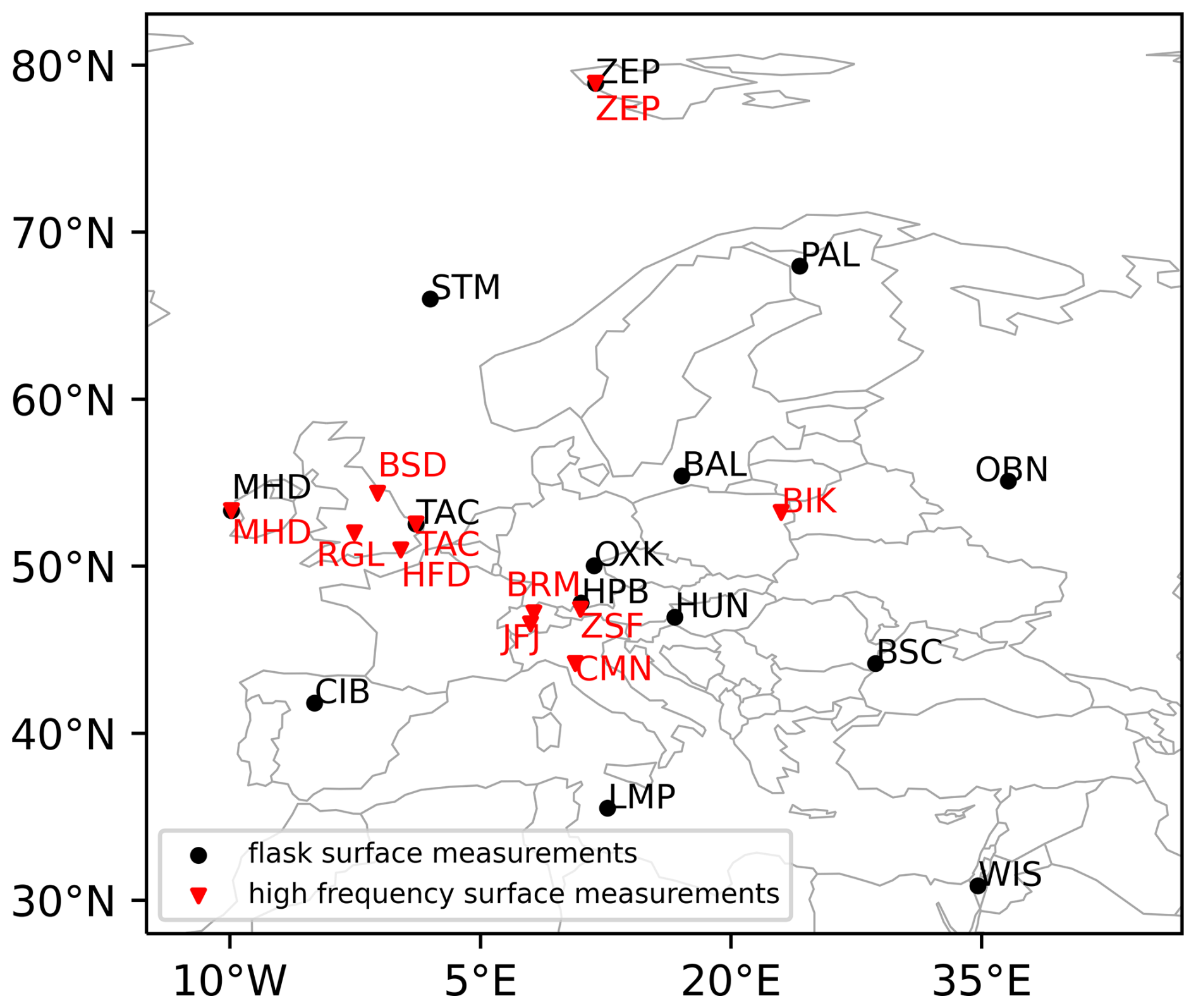
Figure 1 Locations of the observation stations in and around Europe. Stations with continuous surface measurements (BIK, BRM, BSD, CMN, HFD, JFJ, MHD, RGL, TAC, ZEP, ZSF) are represented with red triangles, while surface flask measurements (BAL, BSC, CIB, HPB, HUN, LMP, MHD, OBN, OXK, PAL, STM, TAC, WIS, ZEP) are shown with black dots.

2.2 Emission sensitivities

We use the Lagrangian particle dispersion model (LPDM) FLEXPART 10.4 (Pisso et al., 2019a) in backward mode to simulate the atmospheric transport of SF₆, tracing its movement from the measurement locations back to the emission sources. We neglect loss processes, given that SF₆ is almost inert up to the middle stratosphere. For every observation, we release 50 000 virtual particles continuously over a 3 h interval from the measurement site, tracking their trajectories backward in time for 50 d. The average time spent by these particles in a given emission grid cell determines the sensitivity of the observation to emissions from that specific grid cell. These simulated emission sensitivities form the basis for the atmospheric inversion. We run FLEXPART on a European domain (15° W–40° E, 30–72° N) with an output resolution of 0.25° × 0.25° and on a global domain with an output resolution of 1.0°×1.0°, both with 18 vertical layers of 0.1, 0.5, 1, 2, 3, 4, 5, 7, 9, 11, 13, 15, 17, 20, 25, 30, 40, and 50 km above ground level (a.g.l.) interface heights. The emission sensitivities were calculated solely for the lowest layer, ranging from 0 to 100 m a.g.l., where almost all emissions occur. We utilize hourly ECMWF ERA5² wind fields (Hersbach et al., 2018) to drive the FLEXPART simulations. Specifically, we use 0.25°×0.25° resolution wind fields for the European domain and 0.5°×0.5° wind fields for the global domain, both with 137 vertical levels. Figure 2 shows the simulated annual averaged emission sensitivities for the years (a) 2005 and (b) 2018. In 2018, Europe – particularly northwestern Europe – shows significantly higher emission sensitivities compared to 2005. This increase is largely due to the expansion of the observation network in the UK. As a result, northwestern Europe, including major emitters such as Germany, France, and the UK, became well-monitored, suggesting that substantial improvements in emission estimates through the inversion can be expected over time.

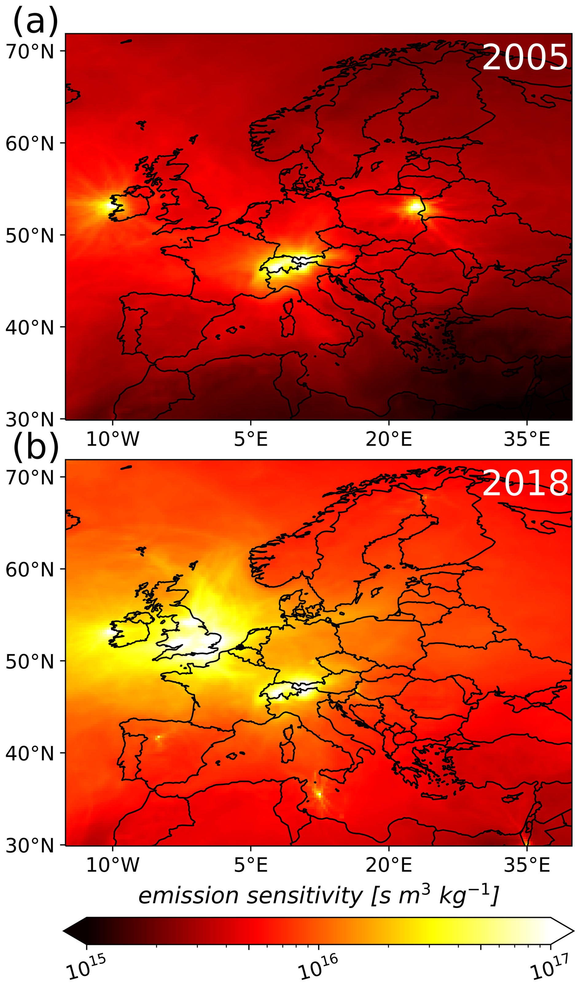
Figure 2 Simulated emission sensitivities for the years 2005 and 2018 in Europe. The displayed values represent the annual sum of FLEXPART calculations. As a result, sites with frequent online observations carry more weight than those relying on flask measurements or observations from mobile platforms.

Baseline

Using the emission sensitivities simulated by FLEXPART, we can link the mole fractions at the receptor to emissions occurring within 50 d of the backward tracking. However, emissions preceding the 50 d period can not directly be captured with these backward simulations. Nevertheless, they still have to be considered when comparing the modeled mole fraction values with the observations. Therefore, all these emission contributions are aggregated in a so-called baseline which must be added to the modeled emission contributions. We apply a Global-Distribution-Based (GDB) method (Vojta et al., 2022) to calculate the baseline, directly from a 3D global mole fraction field. For this, the endpoints of the FLEXPART back-trajectories, are used to determine an observation's sensitivity to the mole fractions at the end of the 50 d simulation period. These sensitivities are simply obtained by dividing the number of trajectories ending in a specific grid cell by the total number of trajectories calculated, as loss processes are omitted. We then multiply the sensitivities with globally 3D gridded SF₆ mole fractions at the time of particle termination and integrate the product over the entire globe. As for the 3D SF₆ field, we employed the data set created by Vojta et al. (2024). Finally, the contributions from emissions occurring during the 50 d FLEXPART simulation period but outside of the European domain are added to the baseline. For a more detailed description of the GDB method and the simulation of the mole fraction fields please see Vojta et al. (2022) and Vojta et al. (2024).

2.3 A priori emissions

We create seven different European SF₆ a priori emission fields with 0.25×0.25° resolution for our inversion domain and for the period 2005 to 2021 that are based on three different bottom-up sources: GAINS, the annual national emission reports to the UNFCCC, and the bottom-up estimates from EDGAR.

• GAINS: We created two a priori emission fields based on the GAINS inventory (Purohit and Höglund-Isaksson, 2017), which is detailed in Vojta et al. (2024). The inventory is available at 0.5° resolution globally and at 0.1° resolution for a European subset covering the EU-27, Iceland, Norway, Switzerland, and the UK. For the first field (GS), we re-gridded the global 0.5° inventory to 0.25° over the European domain by interpolation. For the second field (GS-HR), we used the higher-resolution European dataset, aggregated it to 0.25°, and combined it with the global dataset. While both fields thus share the same resolution (0.25° over Europe), the information content differs: GS is interpolated from coarser data, whereas GS-HR retains detail from the original high-resolution European inventory.

• Reports to the UNFCCC: We utilize the total national SF₆ emissions reported annually to the UNFCCC (United Nations Framework Convention on Climate Change, 2023) and distribute these emissions within each country's borders on a 0.25°×0.25° grid, based on two different proxy datasets: (1) gridded population density (CIESIN, 2018) (UP), or (2) nightlight remote sensing data (Elvidge et al., 2021) (UN). ³

• EDGAR: We use the newly updated, 0.1°×0.1°-gridded annual SF₆ emission inventory EDGARv8.0 (EDGAR, 2023; Crippa et al., 2023) and regrid it to 0.25°×0.25° resolution (E8). In addition, we also utilize the national annual total emissions provided by the previous version EDGARv7.0 (EDGAR, 2022; Crippa et al., 2021), and distribute those totals according to (1) gridded population density (CIESIN, 2018) (E7P) or (2) night light remote sensing (Elvidge et al., 2021) (E7N).

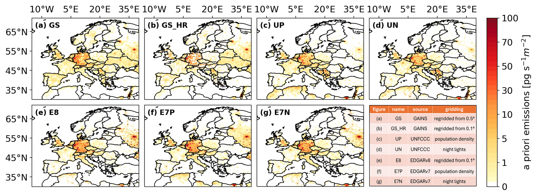
Figure 3 Seven a priori emission fields, shown as an average over the study period 2005–2021: (a) GS (GAINS), (b) GS_HR (GAINS high resolution), (c) UP (UNFCCC reports – population density distribution), (d) UN (UNFCCC reports – night light remote sensing distribution), (e) E8 (EDGARv8), (f) E7P (EDGARv7 – population density distribution), and (g) E7N (EDGARv7 – night light remote sensing distribution). The table in the bottom right corner provides an overview of the ensemble.

To account for contributions from emissions occurring during the 50 d FLEXPART simulation period but outside the European domain, we utilize the global a priori emission fields generated by Vojta et al. (2024). These fields were calculated using the same methodology as our European a priori fields but at a coarser resolution of 1.0×1.0°. Note that this approach results in a single global coarse GAINS inventory.

Figure 3 shows the seven generated European a priori emission fields averaged across the study period from 2005 to 2021. Overall, these emission fields display a relatively similar spatial pattern, especially when compared to the significantly larger differences observed in the global patterns of the bottom-up SF₆ inventories (see Vojta et al., 2024). All European inventories show high SF₆ emissions in central Europe, with Germany being the largest emitter. Notably, a priori emissions are particularly high in western Germany, especially in the area around Cologne. The EDGAR and UNFCCC inventories also highlight substantial emissions in Berlin, which are less prominent in the GAINS inventories. In France, the UNFCCC and EDGAR inventories concentrate emissions in the Paris region, whereas GAINS indicates more dispersed emissions. For the UK, all inventories show the highest emissions in London, with elevated values also occurring in other large cities such as Liverpool, Manchester, and Birmingham. In Italy, the EDGAR inventories estimate higher a priori emissions compared to those from GAINS and UNFCCC. Substantial emissions occur also in the Moscow region, particularly for the EDGAR- and GAINS-based inventories. A detailed discussion on the differences among the a priori inventories and their influence on inversion results are provided in Appendix B.

2.4 Inversion method

We use the Bayesian inversion framework FLEXINVERT+ to find an optimized estimate for European SF₆ emissions based on a priori emissions (Sect. 2.3), atmospheric observations (Sect. 2.1), and atmospheric transport (Sect. 2.2). The framework minimizes the cost function J:

$$\begin{array}{}\text{(1)}& \mathbf{J}\left(\mathit{x}\right)={\displaystyle \frac{\mathrm{1}}{\mathrm{2}}}(\mathit{x}-{\mathit{x}}_{\mathrm{p}}{)}^T{\mathbf{B}}^{-\mathrm{1}}(\mathit{x}-{\mathit{x}}_{\mathrm{p}})+{\displaystyle \frac{\mathrm{1}}{\mathrm{2}}}(\mathbf{Hx}-\mathit{y}{)}^T{\mathbf{R}}^{-\mathrm{1}}(\mathbf{Hx}-\mathit{y}),\end{array}$$

where x and x_p represent the state vector and its a priori values, respectively; y represents the mole fraction enhancements with respect to the baseline, H represents the atmospheric transport operator, B is the a priori error covariance matrix, and R is the observation error covariance matrix. From a Bayesian point of view, J represents the negative logarithm of the a posteriori probability distribution, derived using Bayes' theorem (e.g., Tarantola, 2005). The minimum of the cost function, therefore, defines the maximum of the a posteriori probability distribution, and provides the most probable emission estimate (a posteriori emissions). The analytic solution to minimize J, reads:

$$\begin{array}{}\text{(2)}& \widehat{\mathit{x}}={\mathit{x}}_{\mathrm{p}}+\mathbf{G}(\mathit{y}-{\mathbf{Hx}}_{\mathrm{p}})\end{array}$$

with the defined gain matrix G:

$$\begin{array}{}\text{(3)}& \mathbf{G}={\mathbf{BH}}^T({\mathbf{HBH}}^T+\mathbf{R}{)}^{-\mathrm{1}}\end{array}$$

The a posteriori emission error covariance matrix, $\widehat{\mathbf{B}}$, can also be derived analytically using:

$$\begin{array}{}\text{(4)}& \widehat{\mathbf{B}}=\mathbf{B}-\mathbf{GHB}\end{array}$$

For SF₆, positive fluxes are expected over land, but the inversion may still yield negative a posteriori values in some grid cells. To correct this, we apply the truncated Gaussian method of Thacker (2007), which enforces non-negativity as an inequality constraint. The adjusted fluxes ${\widehat{\mathit{x}}}^{\prime }$ are calculated as

$$\begin{array}{}\text{(5)}& {\widehat{\mathit{x}}}^{\prime }=\widehat{\mathit{x}}+\widehat{\mathbf{B}}{\mathbf{P}}^T{\left(\mathbf{P}\widehat{\mathbf{B}}{\mathbf{P}}^T\right)}^{-\mathrm{1}}\left(\mathit{c}-\mathbf{P}\widehat{\mathbf{x}}\right),\end{array}$$

where $\widehat{\mathit{x}}$ is the original a posteriori estimate, $\widehat{\mathbf{B}}$ the a posteriori error covariance matrix, P the operator identifying violations, and c the constraint vector.

A detailed description of the inversion framework FLEXINVERT+ is provided by Thompson and Stohl (2014), and its application to SF₆ in Vojta et al. (2024). Although we also use observations from outside the European domain and perform FLEXPART simulations globally (with a European nest), the inversions are regional; that is, emissions are optimized only within Europe. Following the inversion process, national emission totals are calculated by aggregating the a posteriori emissions within the respective grid cells of the corresponding country, employing a national identifier grid (CIESIN, 2018).

2.5 Inversion sensitivity studies

A key challenge in inverse modeling is accurately determining the uncertainties of the optimized emissions. Traditionally, the uncertainties in inversion-derived emissions are based on Gaussian error statistics within a Bayesian framework, often relying on a single inversion setup. However, many aspects of the inversion process are based on assumptions and expert judgments. One example is the error covariance matrix used for the a priori emissions. Both the magnitude of this uncertainty as well as its spatiotemporal correlation are usually not available from the bottom-up inventories, and the assumption of a Gaussian distribution is not always well justified. Several studies (e.g., Bergamaschi et al., 2015; Brunner et al., 2017; Chevallier et al., 2019; Locatelli et al., 2013) have demonstrated that the range of emissions derived from different inversion configurations can be significantly larger than the uncertainties calculated by individual inversions. Therefore, in this study, we examine the sensitivity of the inversion results to various inversion settings. Initially, we define 58 distinct inversion settings by systematically varying key parameters, starting from a reference inversion. For the reference inversion, parameter choices were informed by a set of preliminary runs, in which we evaluated chi-squared statistics, and by values reported in previous studies. The settings of the sensitivity tests are applied to each of the 17 years in the study period (2005–2021), resulting in a total of 986 inversions (58×17). Our sensitivity tests include:

• a priori emissions: We use 7 different a priori emission fields based on the inventories of GAINS, the UNFCCC reports and EDGAR (see Sect. 2.3).

• a priori emission uncertainties: In each grid cell, the a priori emission uncertainty is calculated as a fraction of its respective emission value. We test 4 different settings with fractions of 30 %, 50 %, 70 %, and 100 %. Furthermore, different minimum absolute values for the emission uncertainty are tested, controlling the freedom of the algorithm to adjust emissions in grid cells with small a priori values. The seven minimum values tested are $\mathrm{5}\times {\mathrm{10}}^{-\mathrm{14}}$, $\mathrm{1}\times {\mathrm{10}}^{-\mathrm{13}}$, $\mathrm{5}\times {\mathrm{10}}^{-\mathrm{13}}$, $\mathrm{1}\times {\mathrm{10}}^{-\mathrm{12}}$, $\mathrm{5}\times {\mathrm{10}}^{-\mathrm{12}}$, $\mathrm{1}\times {\mathrm{10}}^{-\mathrm{11}}$, and $\mathrm{5}\times {\mathrm{10}}^{-\mathrm{11}}\mathrm{kg}{\mathrm{m}}^{-\mathrm{2}}{\mathrm{h}}^{-\mathrm{1}}$.

• spatial a priori emission uncertainty correlations: FLEXINVERT+ uses an exponential decay function to account for spatial emission uncertainty correlations. We test different spatial scale lengths of 50, 100, 250, 500, 1000 km, as well as a setup with no spatial correlation.

• observation datasets: We test all of the eight observation subsets described in Sect. 2.1.

• observation uncertainties: FLEXINVERT+ assumes a diagonal observation error covariance matrix⁴ and we test different configurations of this uncertainty. The observation uncertainty includes the transport model error projected into the observation space, which is assumed to be the dominant part. Initially, we test constant values of 0.02, 0.04, 0.06, 0.08, and 0.1 ppt. However, it is likely that the model error varies both spatially and temporally. To account for the spatial dependencies, uncertainty estimates are often based on model residuals (the difference between observed and simulated mole fractions) at the measurement stations (e.g. Stohl et al., 2009; Henne et al., 2016). Therefore, we also test two different approaches: (i) using the RMSE between prior modeled and observed values, averaged per station, to determine the observation error, and (ii) estimating the model error from the standard deviation of the a posteriori error distribution through a series of initial inversion runs. In idealized experiments, it has been demonstrated that incorporating temporally varying, flow-dependent uncertainty can enhance the accuracy of emission estimates (Steiner et al., 2024). This transport model ensemble approach, however, requires a lot of resources and lies beyond the scope of our study.

• baseline optimization: FLEXINVERT+ includes an option for baseline optimization, where spatially aggregated contributions are optimized on a coarse grid. Firstly, we test different resolutions for the coarse grid, where the global field is divided into 8, 4, and 2 latitude bands, with northern edges at [−60°, −30°, −15°, 0°, 15°, 30°, 60°, 90°], [−30°, 0°, 30°, 90°], [0°, 90°], respectively. We also run inversions where we optimize one scaling factor for the whole global field. Additionally, we tried different temporal baseline optimization intervals of 15, 30, 45 and 60 d. Furthermore, we test various baseline uncertainty values set to 0.0001, 0.0003, 0.0005, 0.0007, 0.0009, 0.001, 0.01, 0.1, and 1 ppt, and run an inversion without any baseline optimization.

• emission grid: We use emission grids with varying cell sizes, determined by aggregating cells with low emission contributions based on emission sensitivities and a priori emissions (for further details, see Thompson and Stohl, 2014). We test grid configurations with 588, 744, 1992, 2781, 4248, 5370, and 7229 cells, each configuration kept constant over time. Additionally, we implement three dynamic setups where the grid configuration changes each year, with the number of cells ranging from (i) 2781 to 5916, (ii) 3645 to 6599, and (iii) 4151 to 7229.

The set-up of the reference inversion and an overview of all tested inversion configurations are listed in Table 1.

Table 1 Reference inversion set-up and overview of all inversion configurations used in the sensitivity tests.

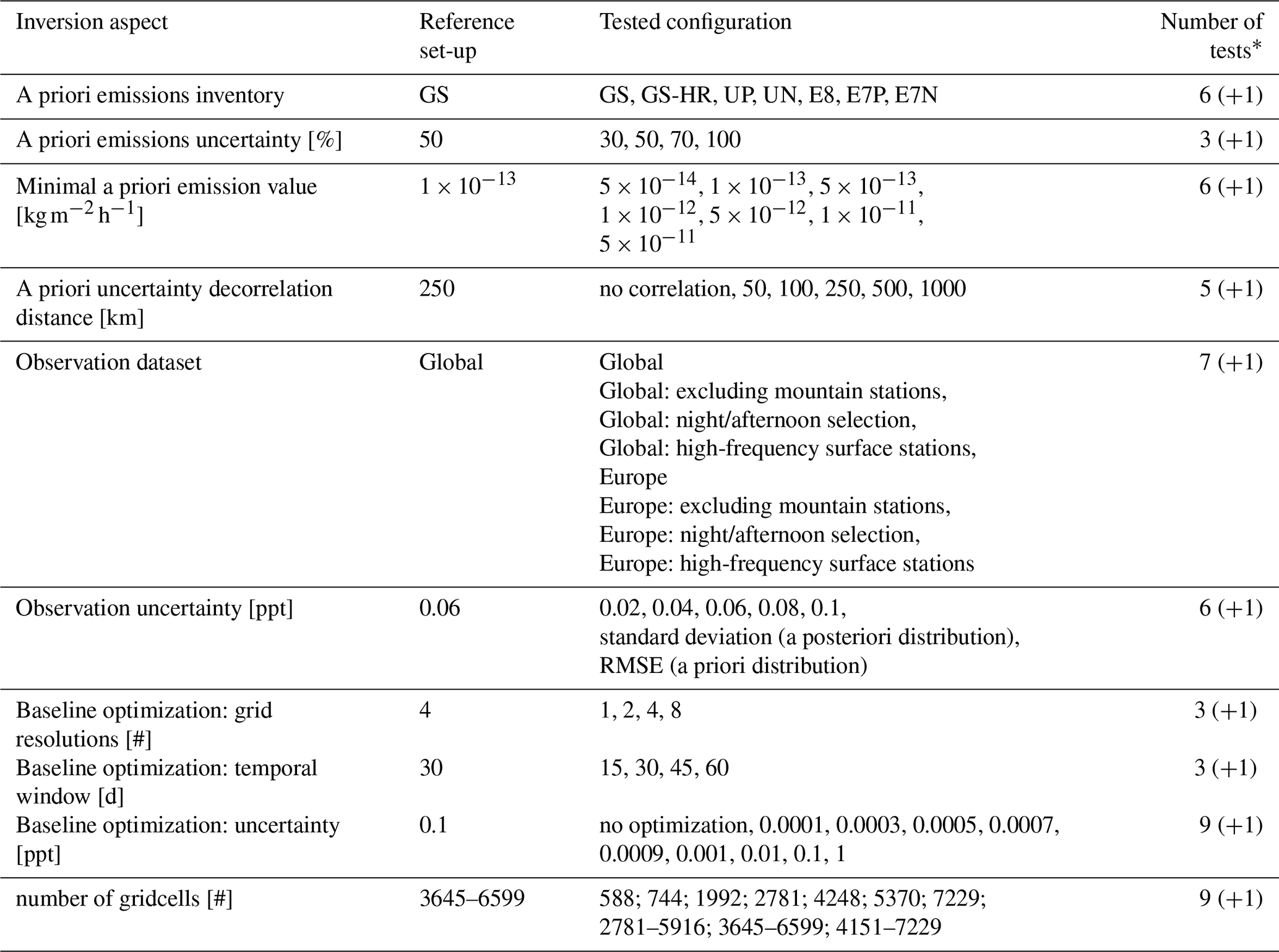
^* (+1) represents the reference inversion setup, which adds one test to the total number for each parameter. However, as the reference inversion is only conducted once, it is only counted once in the overall number of tests.

2.6 Inversion uncertainties

While the sensitivity studies provide insight into how different parameter settings influence the inversion results, the overall uncertainties of the inversion are determined by all these parameters simultaneously. Therefore, in order to accurately quantify the inversion uncertainties, one must apply random variations of these parameters. However, testing all possible combinations is infeasible due to the vast number of permutations. To address this, we employ a Monte Carlo method (e.g. Metropolis et al., 1953) to randomly select and combine inversion parameters, generating an additional 59-member ensemble (1003 inversions). Since the uncertainty distribution of the input parameters is not known, parameters are sampled either continuously from a normal distribution or discretely from a set of predetermined values. The Monte Carlo sampling of the parameter space is performed independently for each parameter. The final selection of parameter ranges for ensemble construction is based on the results of our sensitivity tests. A detailed overview of the ensemble configuration is provided in Table S3, and the choices are discussed in Appendix J. To assess the representativeness of our ensemble and the robustness of our findings, we constructed three additional independent Monte Carlo ensembles using the same parameter ranges: (i) another 59-member ensemble with different parameters compared to the initial ensemble (E59, see Table S4), (ii) an ensemble with half the original size (30 members, E30, see Table S5), and (iii) an ensemble with double the original size (118 members, E118, see Table S6). The results of these ensembles were then evaluated against those of the original ensemble.

3 Results and discussion

3.1 Inversion increments, error reduction, and a posteriori emission distribution

Figure 4 presents (a) the inversion increments (a posteriori minus a priori), (b) the relative error reduction, calculated for each grid cell based on the a priori and a posteriori emission uncertainties as $\mathrm{1}-\frac{\text{a posteriori uncertainty}}{\text{a priori uncertainty}}$, (c) the a posteriori emission distribution, and (d) the a posteriori emissions uncertainty (as calculated using Eq. 4). The results are shown for the reference inversion settings, averaged over the years 2005–2021. Strongly negative increments (Fig. 4a) are found in northern Germany, particularly around Cologne, where a priori emissions are very high (see also Fig. 3). The inversion further reveals large positive increments in southwestern Germany. Other positive increments are evident in France, Italy, the UK, and Russia, whereas negative increments are observed in Switzerland, parts of Scotland, and Israel.

Consistent with the distribution of emission sensitivities (Fig. 2), the largest error reductions (Fig. 4b) are concentrated in central Europe, particularly in well-monitored countries such as the UK, Germany, and Switzerland. Additional areas with notable error reduction include northwestern France and northernmost Italy, Moscow and Israel. Notice that the elevated error reductions in Moscow and Israel are likely a consequence of the relatively high a priori uncertainties in these regions, which give the algorithm more flexibility to adjust emissions. However, since these areas are poorly covered by the observation network, the a posteriori emissions may still be considered unreliable despite the notable error reduction.

Figure 4c reveals particularly high emissions in southwestern Germany, aligning with the findings of Simmonds et al. (2018), who also reported an emission maximum in this region. We also obtain elevated emissions in southern UK, northern and southeastern France, and northern Italy. A posteriori emissions are also high in Moscow and Israel, which, however, show large a posteriori uncertainties, despite the notable uncertainty reductions there (Fig. 4d). As discussed in the Appendix B, the Russian a posteriori emissions are highly sensitive to the choice of a priori emissions, leading to unstable results. In the following sections, we therefore focus on the high-emitting European countries with better observational coverage: the UK, Germany, France, and Italy.

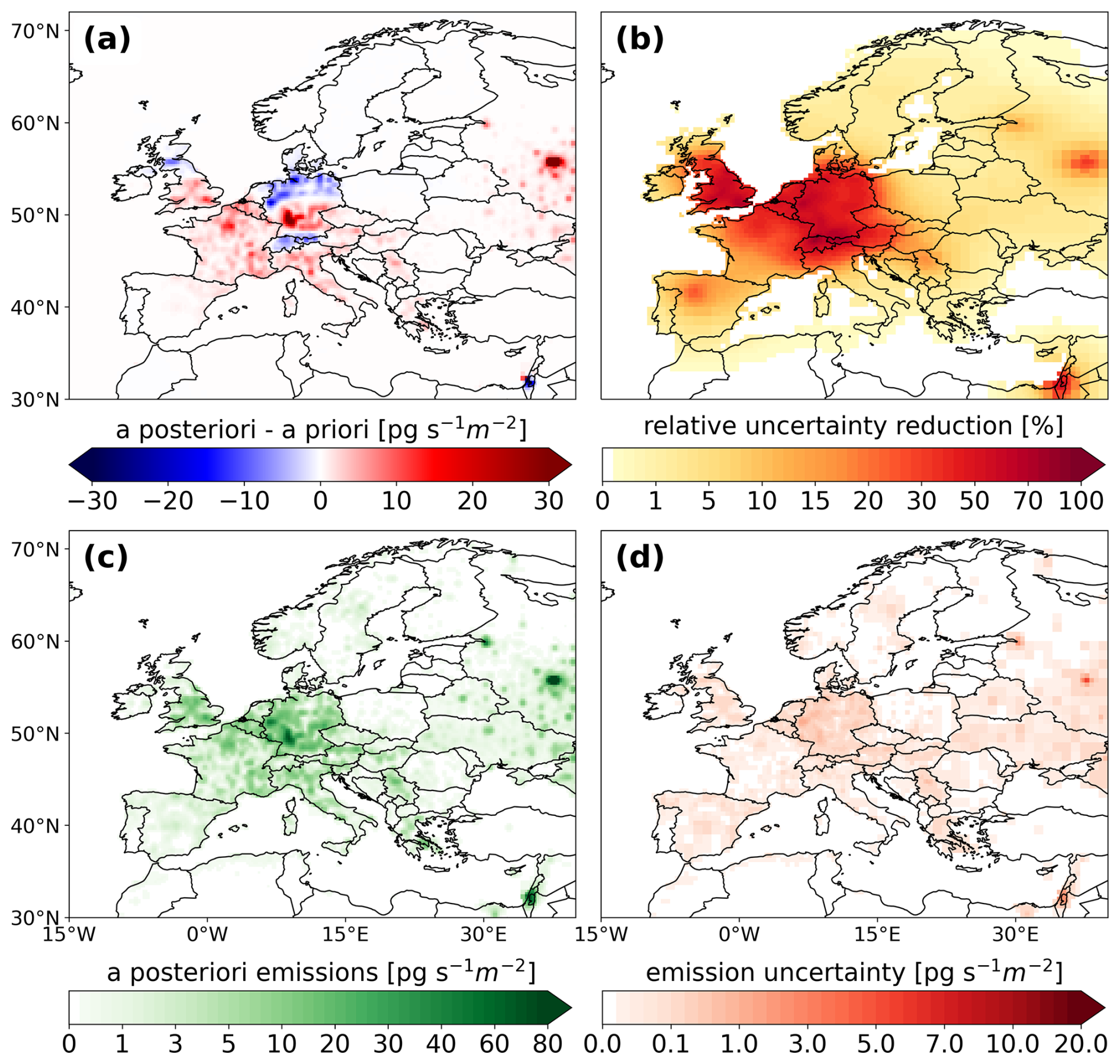
Figure 4 (a) Emission increments from the inversion (a posteriori–a priori), (b) relative error reduction, (c) a posteriori emission distribution, and (d) a posteriori uncertainty obtained for our reference inversion and averaged over all years of the study period 2005–2021.

Table S7 and Fig. S3 demonstrate the statistical improvements at all continuous surface stations, with the sites TAC, HFD, RGL, and BSD showing the largest improvements, thereby highlighting the importance of the UK network expansion.

3.2 Results of the sensitivity tests

The results of all performed sensitivity tests are detailed in the Appendix, organized according to various aspects of the inversion process to assess the sensitivity of the results to each specific setting. Generally, the sensitivities to the different tested settings vary between different years and regions, however, there is one common feature: The better a region is monitored by the observation network, the smaller is the sensitivity to the inversion setting. This is especially apparent in the well-monitored countries like Germany and the UK, where the inversion results are extremely stable across all tested cases (Fig. I1).

In our spectrum of sensitivity tests, inversion results were most sensitive to changes in the spatial correlation length of the a priori emission uncertainty (Fig. D1) and to changes in the baseline uncertainty (Fig. G4). The results were also sensitive to the magnitude of the a priori emission uncertainties (Figs. C1, C3) and observation errors (Fig. F1), with greater sensitivity in poorly monitored areas and minimal sensitivity in well-monitored regions. Additionally, the inversion results were moderately sensitive to the choice of the observation dataset (Fig. E1). Furthermore, our tests suggest that optimizing the baseline across two or more latitudinal bands can lead to substantial differences compared to optimizing the global field with a single scalar (Fig. G1). In contrast, changing the temporal interval for baseline optimization, ranging between 15 and 60 d, had almost no impact on the results (Fig. G3). Also, changing the number of optimized emission grid cells had minimal impact on the results when considering national or European emission totals (Fig. H2). This finding is particularly noteworthy, as computational time is heavily influenced by the number of inversion grid cells.

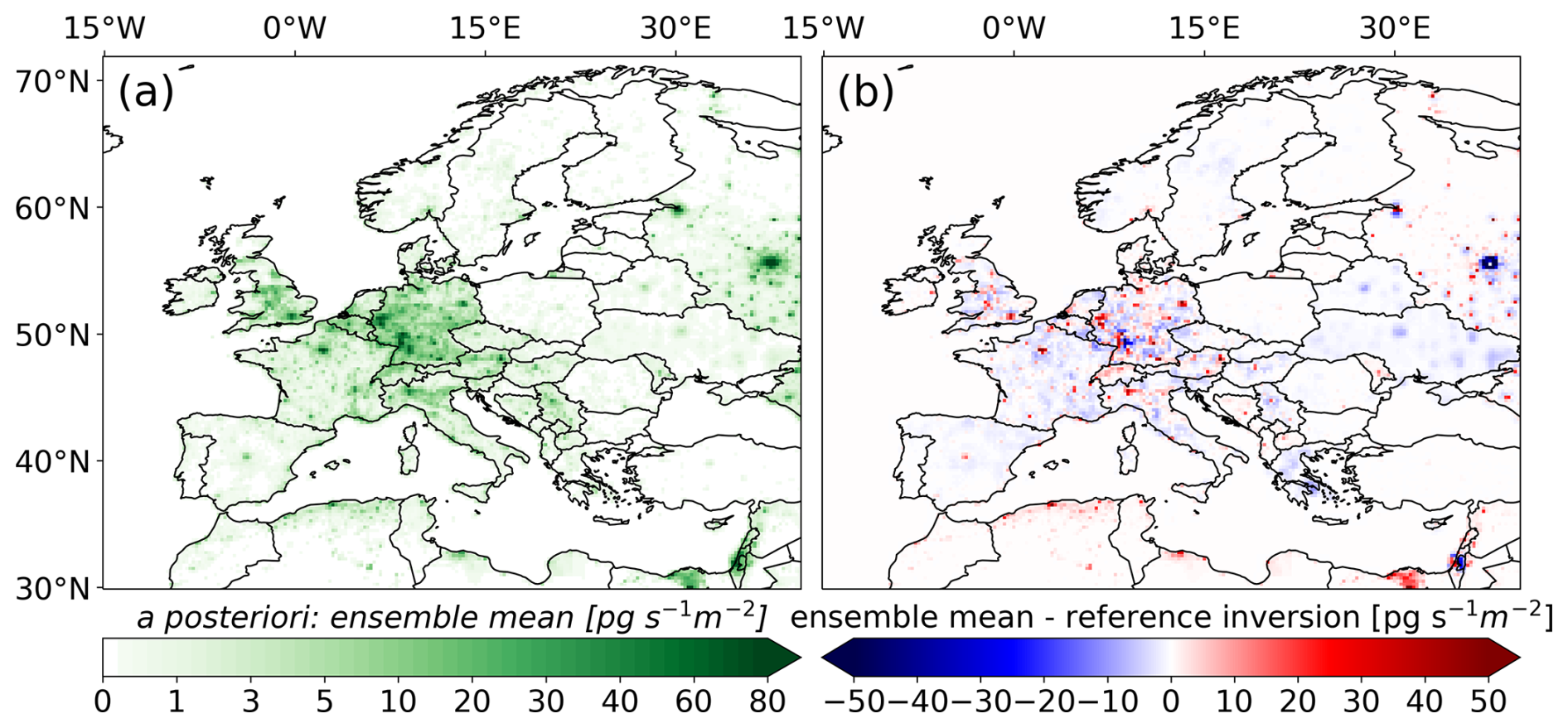
Figure 5 A posteriori emissions: (a) ensemble mean, calculated as the average of all a posteriori emissions from the Monte Carlo ensemble over the study period (2005–2021), and (b) difference between the ensemble mean a posteriori emissions and the a posteriori emissions obtained from the reference inversion.

3.3 A posteriori emission ensemble

Building on the sensitivity tests, we employed a Monte Carlo ensemble presented in Table S3 and calculated the a posteriori emissions for all different settings. The ensemble mean (Fig. 5a) closely resembles the a posteriori emissions of the reference inversion (Fig. 5b), with the largest differences observed in Moscow and Israel, and generally more pronounced discrepancies in larger cities. Note that the ensemble spread (Fig. S2) results in significantly larger uncertainties than the analytically derived uncertainties from the reference inversion (Fig. 4d), which likely fail to capture the full extent of the actual uncertainty.

3.4 Regional emission time series

For the regional emission time series, the inversion results of all members of the Monte Carlo ensemble are shown in Fig. S4 and final results are presented in Table S8, which are defined as ensemble averages across the full set of inversions, with a 2.5th–97.5th percentile uncertainty range for each year. Doubling or halving the ensemble size yielded consistent posterior results, suggesting that the ensemble is sufficiently large to represent the prescribed uncertainty distributions (see Fig. S5).

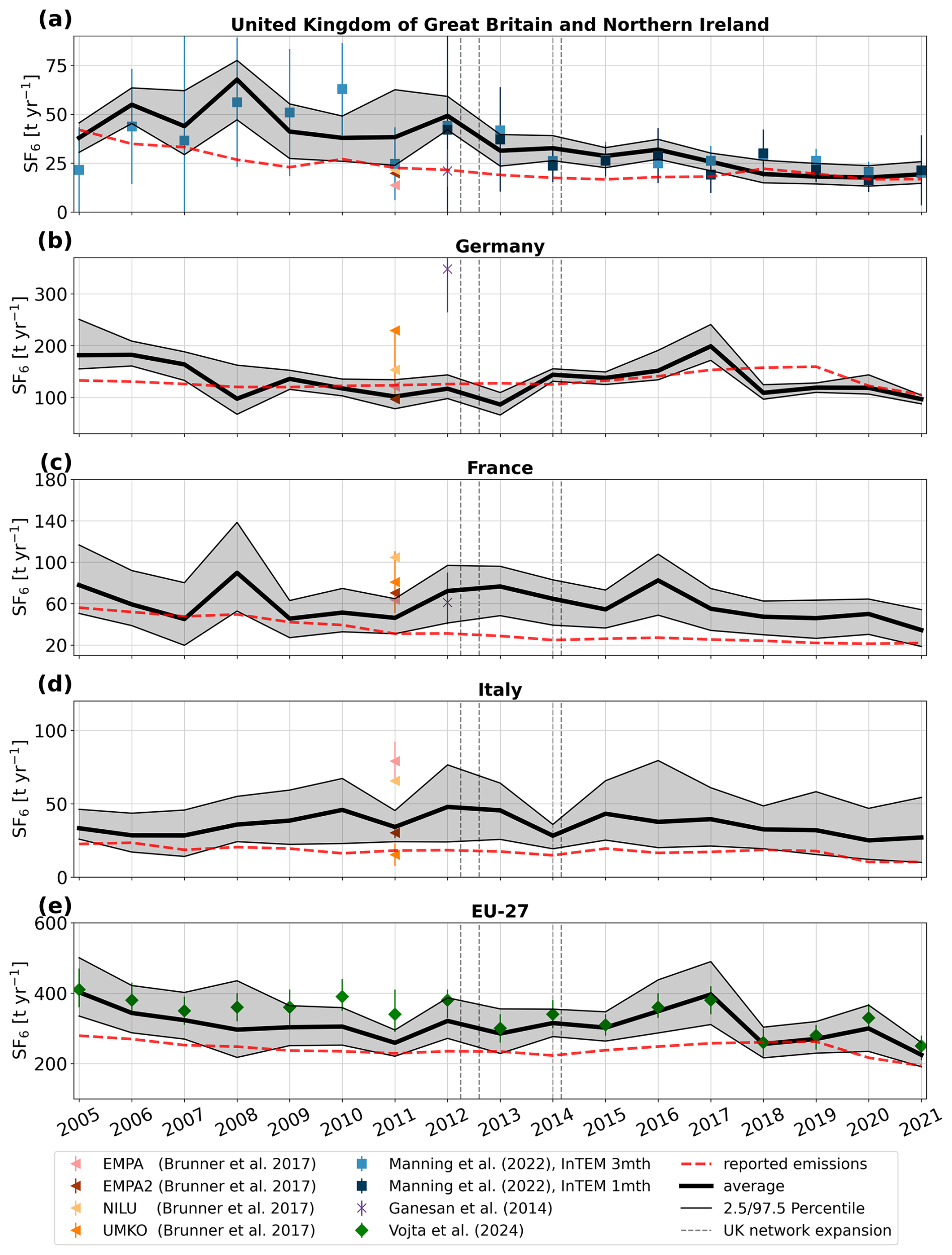
Figure 6 Annual emission time series for (a) the United Kingdom, (b) Germany, (c) France, (d) Italy, and (e) the EU-27. The solid black lines represent the average a posteriori emissions across all performed inversions, and shaded areas indicate the 2.5th–97.5th percentile range for each year. The red dashed line indicates the UNFCCC reported emissions, while results from previous studies are shown with colored markers. The vertical gray lines indicate the times when additional observational data from the expansion of the UK network became available.

Figure 6 shows the a posteriori SF₆ emission time series for (a) the United Kingdom, (b) Germany, (c) France, (d) Italy, and (e) the EU-27. In the UK, SF₆ emissions declined from 38 (31–46) t yr⁻¹ in 2005 to 19 (15–26) t yr⁻¹ by 2021 (Fig. 6a: black solid line), with a substantial drop from 68 (47–77) t yr⁻¹ in 2008 to 19 (15–26) t yr⁻¹ in 2018, corresponding to an average annual decrease of −3.2 t yr⁻¹. The substantial decrease in emissions observed after 2008 is likely a result of the 2006 EU F-gas regulations, with most bans coming into effect in 2008. Although inversion results exceed the reported values (dashed red line) by an average of 69 % between 2005 and 2017, they align closely from 2018 onward. While our results are slightly higher than the estimates of Ganesan et al. (2014) in 2012, and Brunner et al. (2017) in 2011, they are in excellent agreement with the results of Manning et al. (2022) for the whole study period, particularly from 2012 onward, when uncertainties also become significantly smaller. We find equally good agreements when comparing with the a posteriori emissions for northwestern Europe from Manning et al. (2022) (Fig. S6). These good agreements are a particularly noteworthy result, as the inversion system used by Manning et al. (2022) differs significantly from ours. Their approach employs the InTEM inversion technique (Manning et al., 2011, 2021), with a priori emissions uniformly distributed across the country, large a priori emission uncertainties, and inversion intervals of 1 and 3 months (Fig. 6, InTEM 1mth, InTEM 3mth).

In Germany, our results show a decline in emissions from 182 (155–251) t yr⁻¹ in 2005 to 86 (66–109) t yr⁻¹ in 2013. Afterwards, emissions increased significantly, peaking at 199 (172–241) in 2017. This was followed by a sharp drop to 109 (97–125) t yr⁻¹ in 2018, after which emissions stabilized. Over the entire study period, emissions decreased from 182 (155–251) t yr⁻¹ in 2005 to 97 (88–104) t yr⁻¹ in 2021. Overall, the German a posteriori emissions align well with the values reported to the UNFCCC, however, the inversion results reveal distinct emission trends during specific time periods that are not reflected in the reported data. Our results for Germany agree well with three of the four inversions performed in Brunner et al. (2017), but give much lower emissions than those estimated by Ganesan et al. (2014). However, their high estimates were likely a result of the use of excessive German a priori emissions (∼ 650 t yr⁻¹), which were based on the EDGAR v4.2 inventory. Although their German a posteriori emissions were substantially lower than their a priori values, the inversion likely could not fully correct the huge bias present in this version of the EDGAR inventory. As mentioned in Sect. 3.1, the inversion reveals notable regional differences between southern and northern Germany, with significant negative increments in the North and substantial positive increments in the South, especially in the Southwest (Fig. 7a). To further investigate these regional variations, we examine the annual emission trends separately for the North (Fig. 7b) and the South (Fig. 7c), with the division between the two regions at 51° N. In the north, SF₆ emissions decreased substantially, from 112 (79–152) t yr⁻¹ in 2005 to 27 (22–33) t yr⁻¹ by 2021. Note that this decrease in emissions is comparable to the reduction observed in the UK. In contrast, the southern emission trend follows a similar pattern to that of Germany as a whole, including a peak of 166 (125–205) t yr⁻¹ in 2017, followed by a sharp decline to 93 (97–110) t yr⁻¹ in 2018.

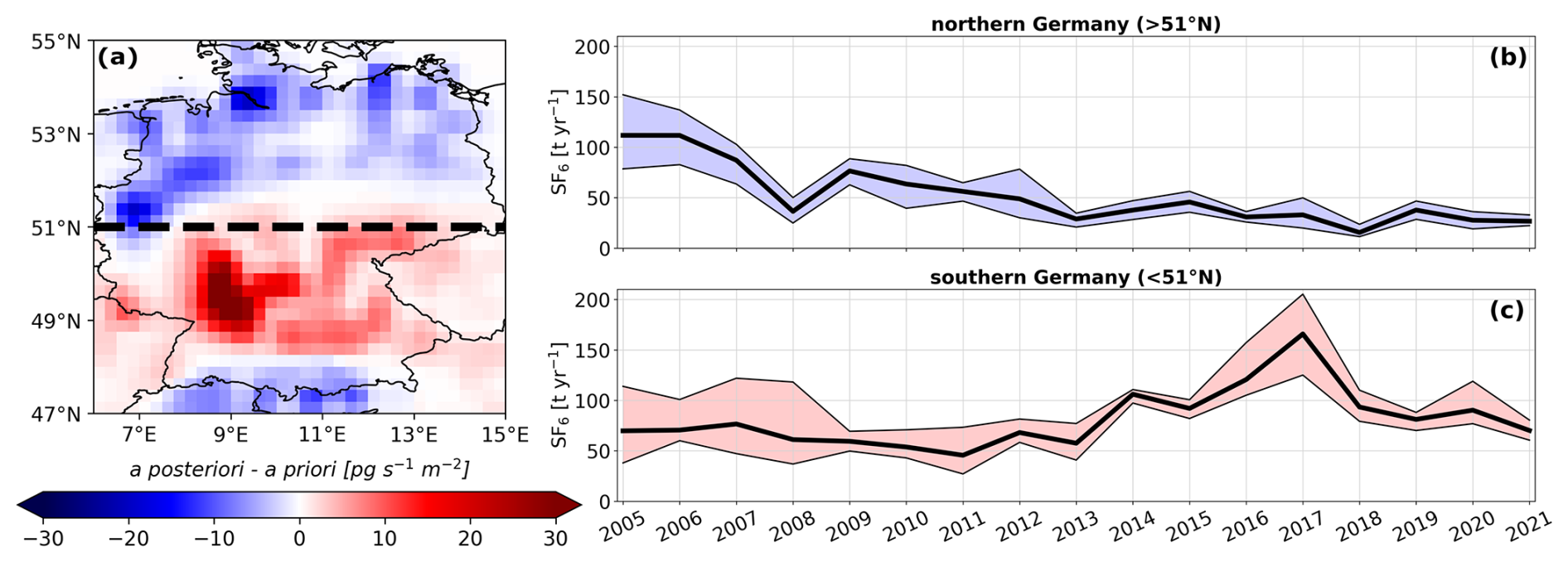
Figure 7 Inversion increments from the reference inversion averaged over the period 2005–2021, with the dashed line indicating our separation of northern and southern Germany (a). Annual emission time series for (b) northern Germany (>51° N) and (c) southern Germany (<51° N). The solid black lines represent the average a posteriori emissions across all performed inversions, and shaded areas indicate the 2.5th–97.5th percentile range for each year.

In France, a posteriori emissions declined from 78 (51–117) t yr⁻¹ in 2005 to 35 (19–54) t yr⁻¹ in 2021, with an average annual decrease of −1.2 t yr⁻¹. Our results exceed the reported values throughout the whole study period by 88 % on average, while they are in good agreement with Ganesan et al. (2014), and the lower estimates of Brunner et al. (2017).

For Italy, our inversion results exhibit large uncertainties in certain years, likely due to limited observational constraint in the central and southern regions. Over the study period, annual a posteriori emissions do not show a clear trend, varying between 25 and 48 t yr⁻¹; however, they exceed the values reported to the UNFCCC by 107 % on average. Our results are within the range of estimates calculated in Brunner et al. (2017), which show a comparable level of uncertainty.

For the aggregated emissions of the EU-27 countries, our results show a decrease in a posteriori emissions from 403 (335–501) t yr⁻¹ in 2005 to 225 (191–260) t yr⁻¹ in 2021, with a substantial emission drop from 396 (311–490) t yr⁻¹ in 2017 to 256 (216–303) t yr⁻¹ in 2018. While until 2017 our results are on average 28 % higher than the reported values, they align well with the reports from 2018 onward. Our results are very similar to the recent estimates of the global SF₆ inversion study of Vojta et al. (2024) after 2012. This is not surprising, as we use the same dataset, atmospheric transport model, and inversion framework. Before 2012, our values are slightly higher from those in Vojta et al. (2024), which we attribute to the improved resolution of our study, the baseline optimization in 8 latitudinal bands, and the definition of our a posteriori emissions as averages over a large inversion ensemble. Our uncertainty intervals, defined as the 2.5th–97.5th percentile uncertainty range across the performed inversions, are much wider than those reported in Vojta et al. (2024). Their uncertainty intervals, in contrast, were based on the minimum and maximum uncertainty limits across inversion results using only six different a priori emission inventories.

Note that the temporal pattern of EU-27 a posteriori emissions closely resembles the German pattern after 2012, as Germany is the largest European SF₆ emitter. The high emissions in Southern Germany (Fig. 7c), in particular, seem to have a large influence on the total EU-27 emission variations. We interpret the decline in SF₆ emissions as a consequence of the EU F-gas regulations introduced in 2006 (EU, 2006) and 2014 (EU, 2014). As suggested by Vojta et al. (2024), the sharp drop in EU-27 emissions from 2017 to 2018 might indicate an immediate effect of the 2014 regulation, which mandated that new electrical switchgear be put into service starting in 2017 and banned the use of SF₆ in recycling magnesium die-casting alloys from 2018. It seems that strong actions were taken particularly in south Germany when the 2014 regulation came into effect.

The vertical dashed gray lines in Fig. 6 indicate the times when additional observational data from the expansion of the UK network became available (RGL: March 2012, TAC July 2012, HFD: January 2014, BSD: February 2014). Consistent with our sensitivity studies, we observe that the additional observations noticeably reduce emission uncertainties in the UK. Similarly, this effect is observed in Germany, particularly in the north (see Fig. 7). However, the large southern emissions in 2016 and 2017 led to elevated uncertainties, primarily due to the use of different observational datasets (see Appendix E), making them an exception to this trend. Our tests cover a broad range of key inversion settings; however, additional factors such as alternative atmospheric transport models, wind field data, or inversion frameworks could lead to further deviations from our results. Nevertheless, the excellent agreement of the emissions in the UK and northwestern Europe (Figs. 6a and S6) with those reported by Manning et al. (2022), particularly after the network expansion, might suggest that, with a dense monitoring network, inversion results remain stable even when these factors change.

4 Conclusions

In this study, we estimated European SF₆ emissions from 2005 to 2021, focusing on the largest emitters – the United Kingdom, Germany, France, Italy – and the aggregated EU-27 emissions. We conducted an extensive ensemble of 987 inversions to test the sensitivity of the results to various settings within the inversion framework. Building on this, we performed an additional 1003 inversions, using Monte Carlo methods to randomly select and combine inversion parameters, allowing us to quantify the uncertainties in the inversion results. The key findings of our study are as follows:

• We observe a decline in SF₆ emissions across most of the studied countries, as well as in the aggregated EU-27 emissions, over the period from 2005 to 2021. We interpret these declining emissions as a direct consequence of the EU F-gas regulations in 2006 and 2014. While our results are consistent with previous inversion studies, they indicate clearly that European countries generally underreport their SF₆ emissions to the UNFCCC.

• In the UK, SF₆ emissions decreased from 38 (31–46) t yr⁻¹ in 2005 to 19 (15–26) t yr⁻¹ by 2021, with a considerable decrease from 68 (47–77) t yr⁻¹ in 2008 to 19 (15–26) t yr⁻¹ in 2018, corresponding to an average annual decrease of −3.2 t yr⁻¹. While the inversion results are, on average, 69 % higher than the values reported to UNFCCC prior to 2018, they align closely for the most recent investigated years, 2018–2021.

• Germany is the largest SF₆ emitter in Europe. Over the study period, emissions decreased from 182 (155–251) t yr⁻¹ in 2005 to 97 (88–104) t yr⁻¹ in 2021, aligning relatively well with UNFCCC-reported values. Our results suggest that emission inventories overestimate emissions in northern Germany and underestimate emissions in southern Germany (division at 51° N). Emissions in northern Germany declined from 112 (79–152) t yr⁻¹ in 2005 to 27 (22–33) t yr⁻¹ in 2021, while emissions in southern Germany showed a distinct peak of 166 (125–205) t yr⁻¹ in 2017, followed by a sharp decline to 93 (97–110) t yr⁻¹ in 2018.

• In France, a posteriori emissions decreased from 78 (51–117) t yr⁻¹ in 2005 to 35 (19–54) t yr⁻¹ in 2021, on average exceeding the reported values by 88 %.

• In Italy, annual a posteriori emissions show no clear trend, varying between 25 and 48 t yr⁻¹ throughout the study period, On average, emissions exceeded the reported UNFCCC values by 107 %.

• For the aggregated emissions of the EU-27 countries, our results show a decrease in a posteriori emissions from 403 (335–501) t yr⁻¹ in 2005 to 225 (191–260) t yr⁻¹ in 2021, with a substantial emission drop from 396 (311–490) t yr⁻¹ in 2017 to 256 (216–303) t yr⁻¹ in 2018. On average, our results are 28 % higher than the reported values before 2018, however, after the drop in 2018, they align better with the reported values from 2018 to 2021. As noted by Vojta et al. (2024), this drop is likely a direct result of the 2014 regulation, which mandated that new electrical switchgear containing SF₆ be put into service starting in 2017 and prohibited the use of SF₆ in recycling magnesium die-casting alloys from 2018. Additionally, we notice that the drop closely mirrors the decline in emissions in southern Germany over the same period, suggesting that strong actions were likely taken there when these regulations came into force.

• Our large ensemble of sensitivity tests shows that as the observational coverage in a region increases, the inversion results become less sensitive to the various a priori settings that are subject to uncertainty. This becomes especially apparent in countries like Germany and the UK, where the inversion results stabilize substantially following the expansion of the British observation network. The good agreement of emissions in the UK and northwest Europe after 2014 with Manning et al. (2022) further suggests that factors not tested in this study – such as alternative atmospheric transport models, meteorological data driving the models, or different inversion frameworks – become less significant when a dense monitoring system is in place. It also demonstrates the considerable potential of inverse modeling to provide reliable emission estimates and underscores the importance of extending the existing network (e.g. Weiss et al., 2021; Leip et al., 2017).

In addition, our sensitivity tests, described in detail in the Appendix, reveal the following:

• Inversion results demonstrate high sensitivity to the choice of spatial correlation length for the a priori emission uncertainty, ranging from 0 to 1000 km. While the optimal correlation length depends on the specific problem, a range around 250 km appears to be a good compromise between providing sufficient constraint on emissions and maintaining the inversion’s ability to resolve regional emission patterns. In contrast, correlation lengths of 500 km, 1000 km, or the absence of correlation led to substantial differences. When emission uncertainties are assumed to be entirely uncorrelated, the inverse problem becomes relatively ill-determined. However, excessively large correlation lengths prevent the inversion's ability to capture regional emission patterns.

• Inversion results were also significantly influenced by the choice of baseline uncertainty, particularly within the range of 0 to 0.0003 ppt. Although increasing the uncertainty further led to additional changes, the effect gradually diminished, stabilizing between 0.01 and 0.1 ppt. We recommend ensuring the baseline uncertainty is not underestimated, as this can significantly impact the results.

• Optimizing the baseline using two or more latitudinal bands most likely yields better results than optimizing the entire field with a single scalar. Therefore, we recommend optimizing the baseline in at least two latitudinal bands, particularly for species such as SF₆, which exhibit a strong latitudinal gradient and large interhemispheric differences. In contrast, the choice of temporal interval for baseline optimization (ranging from 15 to 60 d) had minimal impact on the results.

• The number of optimized emission grid cells, ranging from 588 to 7229, had minimal impact on the obtained national total emissions. Given that the computational time for an inversion is strongly influenced by the number of grid cells optimized, we recommend conducting prior sensitivity tests related to the grid configuration. This approach could help conserve significant computational resources using a coarser grid where appropriate.

• Results were sensitive to variations in both a priori emission uncertainties and observation errors, with greater sensitivity in poorly monitored areas and minimal impact in well-monitored regions. We recommend conducting sensitivity tests on these uncertainties to improve the accuracy of uncertainty estimates in inversion results.

• Inversion results showed moderate sensitivity to the choice of the observation dataset and a priori emission fields. Again, we suggest using multiple a priori emission datasets and observational datasets to improve the reliability of uncertainty estimates in the inversion results.

Our study indicates that regulations, such as those implemented by the EU for F-gases, can have a significant positive impact on regional GHG emissions. It will be interesting to observe how the EU's new 2024 F-gas regulation will further reduce European SF₆ emissions in the future. Considering the substantial regional emission reductions observed, Europe could serve as a role-model for effectively reducing SF₆ emissions. Similar regulations would be crucial in other regions for mitigating global SF₆ emissions (Vojta et al., 2024; An et al., 2024). Furthermore, expanding observation networks – similar to the dense British network – should be a top priority, as this would greatly reduce uncertainties in top-down emission estimates derived from inverse modeling. These improved estimates could then be incorporated into national reports, as already done by Switzerland, the UK, and Australia (e.g. Rypdal et al., 2005; Leip et al., 2017), substantially enhancing our understanding of GHG emissions.

Appendix A: Evaluation of inversion setup sensitivities

This Appendix presents the results from various inversion setups, organized by specific aspects of the inversion process to examine the sensitivity of results to each setting. We display emission time series for four major emitting countries: the UK, Germany, France, and Italy, as well as for the aggregated EU-27 emissions. Where relevant, we include a priori or a posteriori emission maps, as well as inversion increments (a posteriori–a priori), either averaged over the entire study period or focused on specific years or countries. Additionally, we provide error reduction information for one particular case to provide further insight. The reference inversion is indicated by a black frame around the respective inversion maps or by a thick line in the case of emission time series.

Appendix B: Sensitivity to the a priori emissions

We employ seven different a priori emission fields derived from the GAINS inventories, UNFCCC reports, and EDGAR data (see Sect. 2.3 and Fig. 3). Figure B1 shows the inversion increments averaged throughout the entire study period when using different a priori inventories. While in some regions the increments vary in magnitude, they show a very similar pattern across all cases. We see negative increments in northern Germany, especially in the area around Cologne, where a priori emissions tend to be very high. The UNFCCC- and EDGAR-based inversions also show strong negative increments in Berlin, where the a priori estimates are high. All tests show large positive increments in southwest Germany, positive increases in France, Italy, and the UK, and negative increments in Switzerland. Notice that the EDGAR-based inventories E7P and E8 show negative increments in the area of Moscow, in contrast to the other inventories. For a more detailed analysis, Fig. B2 presents the a priori (a–g) and a posteriori (h–n) emissions in the Moscow region, averaged over the study period 2005–2021. While the a priori emissions exhibit significant differences, the a posteriori emissions show better agreement. However, substantial uncertainties persist due to the use of different a priori inventories, even after the correction from the inversion.

Figure B3 presents the a posteriori emission time series for the UK, Germany, France, Italy, and the EU-27 based on different a priori emission inventories. In the UK (Fig. B3a), differences in the a posteriori emissions due to different a priori inventories are relatively large in the early years of the study period, but decrease significantly toward the end, particularly after 2011, when the British observation network was expanded. Similarly, the differences in the French a posteriori SF₆ emissions (Fig. B3c) decrease over the study period; however, this is less evident than for the UK. In Germany (Fig. B3b), the sensitivity to different inventories remains relatively low throughout the study period. This is particularly noteworthy toward the end of the period, when a priori inventories show considerable differences, indicating substantial improvements from the optimization. In Italy (Fig. B3d), a priori emissions from the different inventories are quite similar until 2017, leading to relatively closely aligned a posteriori emissions. However, toward the end of the time series, the a priori estimates start to diverge, resulting in larger differences in the corresponding a posteriori emissions, especially in 2021. This divergence is likely related to the fact that Monte Cimone provided observations only until 2017, after which constraints on Italian emissions were substantially reduced. A closer examination of the year 2021 reveals significantly higher a priori emissions and positive increments close to Milan for the EDGAR- and UNFCCC-based inventories (Fig. B4c–g, j–n), compared to the lower values from the GAINS-based inventory (Fig. B4a, b and h, i). The larger increments observed for higher a priori values can most likely be attributed to the definition of the a priori emission uncertainty, giving the algorithm more freedom in grid cells with high a priori values. Consequently, emissions that are high but still underestimated are easier to correct than those that are even lower. This might indicate that our uncertainties for individual grid cells might be generally too small and that our posterior uncertainties, as estimated using the analytical method, might be significantly underestimated at the national level. The aggregated a posteriori emissions of the EU-27 countries (Fig. B3e) show a relatively low dependence on the a priori inventory, with differences across cases decreasing up to 2018. After 2018 differences slightly grow again, which can be attributed to the strongly diverging a priori inventories.

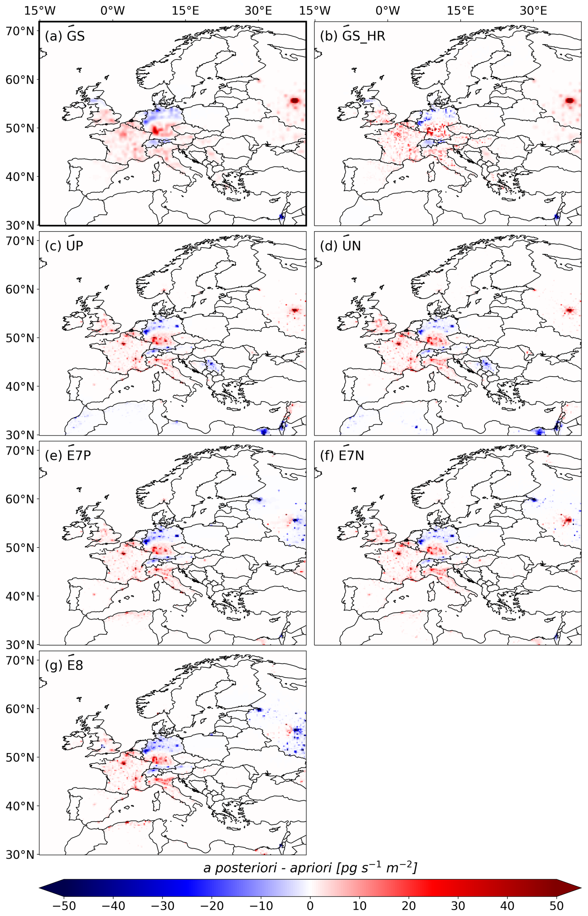
Figure B1 Inversion increments (a posteriori–a priori) averaged over the entire study period (2005–2021), shown for different a priori emission inventories: (a) GS, (b) GS_HR, (c) UP, (d) UN, (e) E7P, (f) E7N, (g) E8.

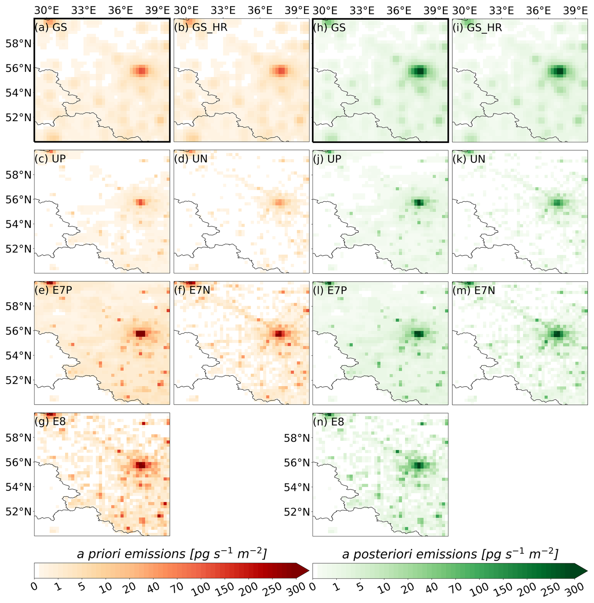
Figure B2 Moscow region: a priori emissions (left) and a posteriori emissions averaged over the entire study period (2005–2021) using different inventories: (a, h) GS, (b, i) GS_HR, (c, j) UP, (d, k) UN, (e, l) E7P, (f, m) E7N, (g, n) E8.

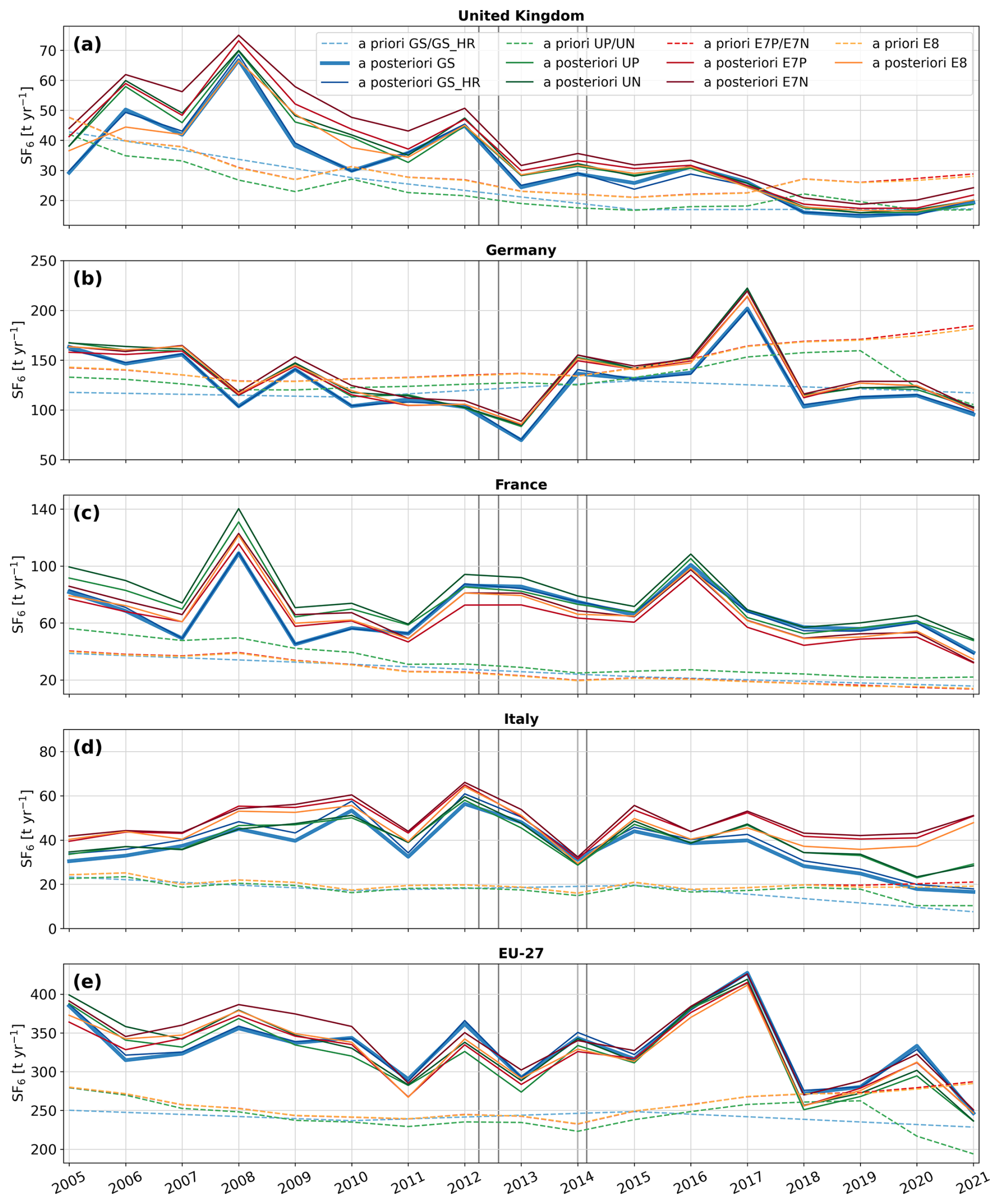
Figure B3 Annual emission time series for (a) the United Kingdom, (b) Germany, (c) France, (d) Italy, and (e) the EU-27, using different a priori emissions inventories. The colored solid lines (light blue: GS, dark blue: GS_HR, light green: UP, dark green: UN, light red: E7P, dark red: E7N, orange: E8 ) represent the a posteriori emissions derived using different a priori emission inventories, which are shown by the dashed lines in corresponding colors.The vertical gray lines indicate the times when additional observational data from the expansion of the UK network became available.

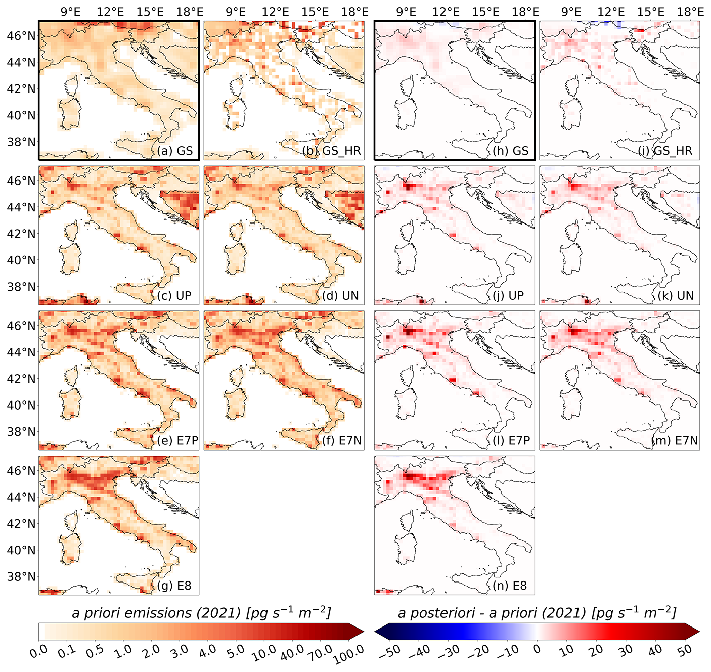
Figure B4 A priori emissions (left-hand side) and emission increments (right-hand side) in Italy for the year 2021, shown for different a priori emission inventories: (a, h) GS, (b, i) GS_HR, (c, j) UP, (d, k) UN, (e, l) E7P, (f, m) E7N, (g, n) E8.

Appendix C: Sensitivity to the a priori emission uncertainty

In FLEXINVERT+, the a priori emission uncertainty in each grid cell is calculated as a fraction of the corresponding emission value. We evaluate four different settings with fractions of 30 %, 50 %, 70 %, and 100 %, with the inversion results presented in Fig. C1. As the a priori emission uncertainty increases from 30 % to 100 %, the constraint on the a priori emissions weakens, allowing the a posteriori emissions to deviate further from their a priori values. Notable, the step from 30 % to 50 % results in the largest differences, while the step from 70 % to 100 % causes only minor differences. Using prior uncertainties of 30 %, 50 %, and 70 % resulted in reduced chi-square values close to 1 (1.12, 0.87, and 0.70, respectively, averaged over all study years). By contrast, the value of 0.55 obtained for 100 % uncertainty might indicate an overestimation of the a priori errors. In general, we observe little sensitivity to the a priori emissions in Germany (Fig. C1b) and the UK (Fig. C1a). For France, Italy, and the aggregated EU-27 emissions, the sensitivity to the a priori uncertainty generally decreases over time, with differences becoming relatively small after 2014.

Furthermore, we test various minimum emission uncertainty values to allow the algorithm to adjust emissions in grid cells with very small a priori values. The seven minimum values tested are $\mathrm{5}\times {\mathrm{10}}^{-\mathrm{14}}$, $\mathrm{1}\times {\mathrm{10}}^{-\mathrm{13}}$, $\mathrm{5}\times {\mathrm{10}}^{-\mathrm{13}}$, $\mathrm{1}\times {\mathrm{10}}^{-\mathrm{12}}$, $\mathrm{5}\times {\mathrm{10}}^{-\mathrm{12}}$, $\mathrm{1}\times {\mathrm{10}}^{-\mathrm{11}}$, and $\mathrm{5}\times {\mathrm{10}}^{-\mathrm{11}}\mathrm{kg}{\mathrm{m}}^{-\mathrm{2}}{\mathrm{h}}^{-\mathrm{1}}$, with the corresponding uncertainty distribution illustrated in Fig. C2. Figure C3 shows the respective inversion results for (a) the United Kingdom, (b) Germany, (c) France, (d) Italy, and (e) the EU-27. For the smaller minimum emission uncertainties between $\mathrm{5}\times {\mathrm{10}}^{-\mathrm{14}}$ and $\mathrm{1}\times {\mathrm{10}}^{-\mathrm{12}}\mathrm{kg}{\mathrm{m}}^{-\mathrm{2}}{\mathrm{h}}^{-\mathrm{1}}$ (red, blue, green, and purple), the inversion results remain very similar. However, as the minimum emission uncertainty further increases, the a posteriori emissions deviate more significantly from the a priori values. Similar to the previous tests, the inversion results are very stable for the UK and Germany, while the sensitivity in France decreases notably from 2012 to 2021. In contrast, Italy’s a posteriori emissions exhibit relatively large differences in some years (including after 2014), likely due to limited observational coverage in southern Italy. These differences are particularly evident for the highest tested value of $\mathrm{5}\times {\mathrm{10}}^{-\mathrm{11}}\mathrm{kg}{\mathrm{m}}^{-\mathrm{2}}{\mathrm{h}}^{-\mathrm{1}}$ (light orange). In case of the aggregated EU-27 a posteriori emissions, the highest tested value of $\mathrm{5}\times {\mathrm{10}}^{-\mathrm{11}}\mathrm{kg}{\mathrm{m}}^{-\mathrm{2}}{\mathrm{h}}^{-\mathrm{1}}$ also leads to considerably higher interannual variability compared to the other tested values. To further investigate how the minimum a priori uncertainty affects the inversion, we also show the 2012 European inversion increments for the same seven values in Fig. C4, since we observe the biggest differences in this year. Consistent with Fig. C3, increments are similar for minimum values between $\mathrm{5}\times {\mathrm{10}}^{-\mathrm{14}}$ and $\mathrm{1}\times {\mathrm{10}}^{-\mathrm{12}}\mathrm{kg}{\mathrm{m}}^{-\mathrm{2}}{\mathrm{h}}^{-\mathrm{1}}$. However, as the minimum a priori uncertainty further increases, the emission increment patterns begin to change. The increments become less localized and spread over larger areas, especially apparent in France. This shift occurs because the a priori uncertainty becomes similar across most grid cells (see Fig. C2), compelling the algorithm to distribute increments more evenly. For poorly observed areas, such as regions around the Black Sea, the large a priori uncertainties result in excessively strong positive increments. This behavior contrasts with well-covered areas such as Germany or the UK, where almost no differences are observed until the minimum value reaches $\mathrm{5}\times {\mathrm{10}}^{-\mathrm{11}}\mathrm{kg}{\mathrm{m}}^{-\mathrm{2}}{\mathrm{h}}^{-\mathrm{1}}$ (g), at which point the results become noisy in the whole domain, indicating that the inversion becomes poorly constrained. At this point the inversion problem becomes rather ill-posed, producing widespread artifacts.

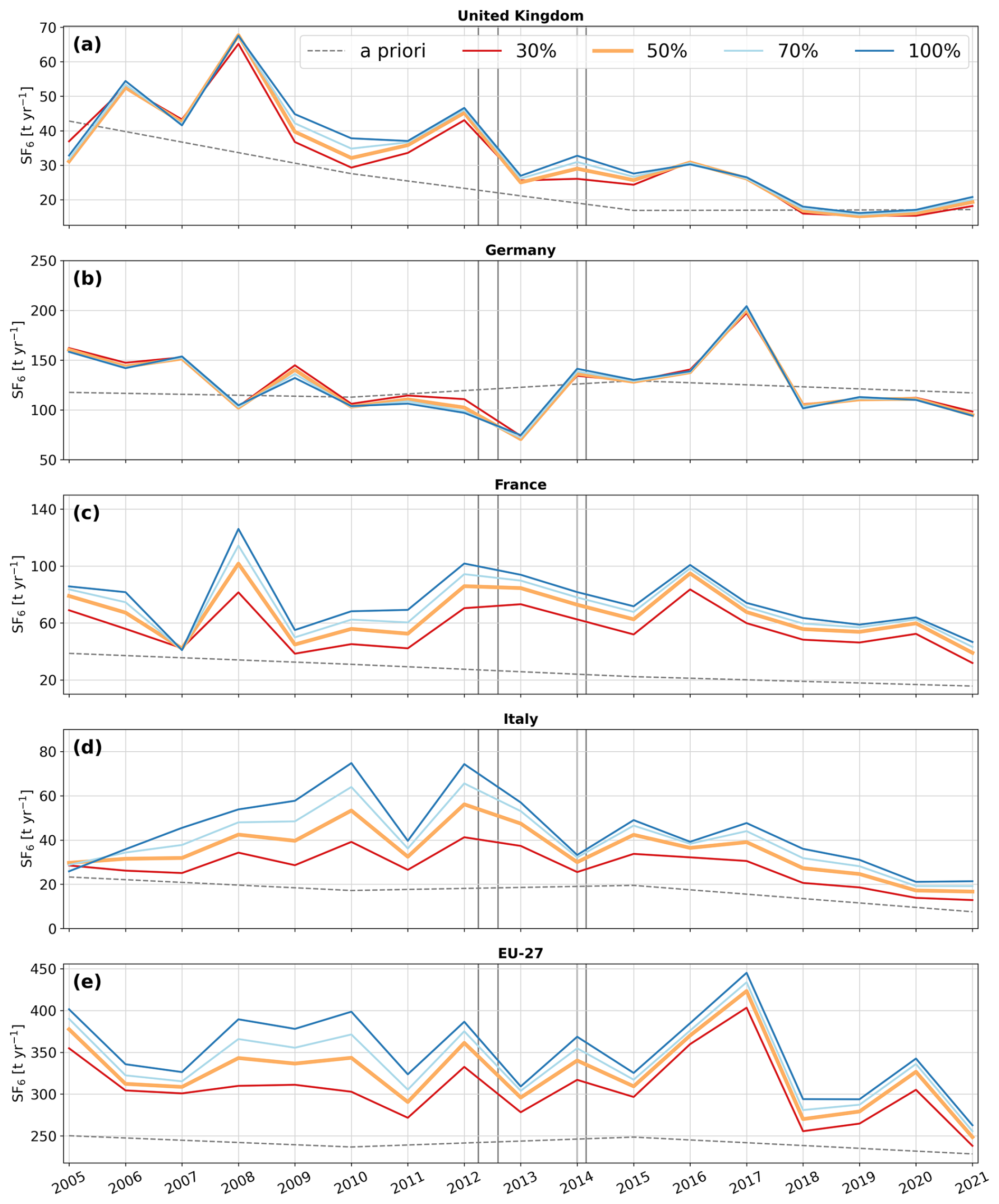
Figure C1 Annual emission time series for (a) the United Kingdom, (b) Germany, (c) France, (d) Italy, and (e) the EU-27, using differnt settings of a priori emissions uncertainties, defined as a fraction of the corresponding emission value in each grid cell. The colored solid lines (red: 30 %, orange: 50 %, light blue: 70 %, and blue: 100 % of the respective emission value) represent the a posteriori emissions derived using the different settings and the gray dashed line shows the a priori emissions. The vertical gray lines indicate the times when additional observational data from the expansion of the UK network became available.

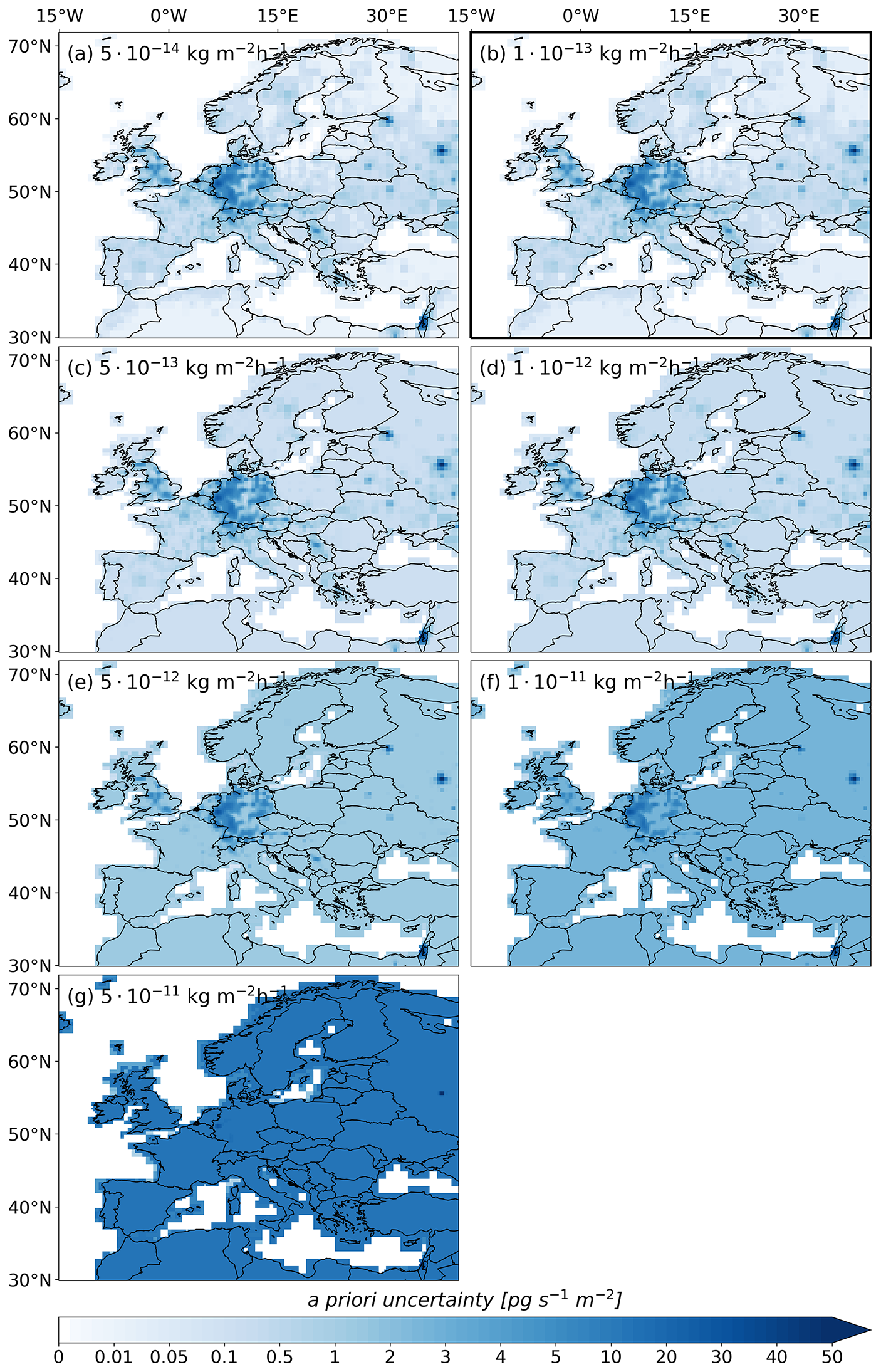
Figure C2 A priori emission uncertainties averaged over the entire study period (2005–2021), shown for different tested minimal a priori emission uncertainty values (a) $\mathrm{5}\times {\mathrm{10}}^{-\mathrm{14}}\mathrm{kg}{\mathrm{m}}^{-\mathrm{2}}{\mathrm{h}}^{-\mathrm{1}}$, (b) $\mathrm{1}\times {\mathrm{10}}^{-\mathrm{13}}\mathrm{kg}{\mathrm{m}}^{-\mathrm{2}}{\mathrm{h}}^{-\mathrm{1}}$, (c) $\mathrm{5}\times {\mathrm{10}}^{-\mathrm{13}}\mathrm{kg}{\mathrm{m}}^{-\mathrm{2}}{\mathrm{h}}^{-\mathrm{1}}$, (d) $\mathrm{1}\times {\mathrm{10}}^{-\mathrm{12}}\mathrm{kg}{\mathrm{m}}^{-\mathrm{2}}{\mathrm{h}}^{-\mathrm{1}}$, (e) $\mathrm{5}\times {\mathrm{10}}^{-\mathrm{12}}\mathrm{kg}{\mathrm{m}}^{-\mathrm{2}}{\mathrm{h}}^{-\mathrm{1}}$, (f) $\mathrm{1}\times {\mathrm{10}}^{-\mathrm{11}}\mathrm{kg}{\mathrm{m}}^{-\mathrm{2}}{\mathrm{h}}^{-\mathrm{1}}$, and (g) $\mathrm{5}\times {\mathrm{10}}^{-\mathrm{11}}\mathrm{kg}{\mathrm{m}}^{-\mathrm{2}}{\mathrm{h}}^{-\mathrm{1}}$).

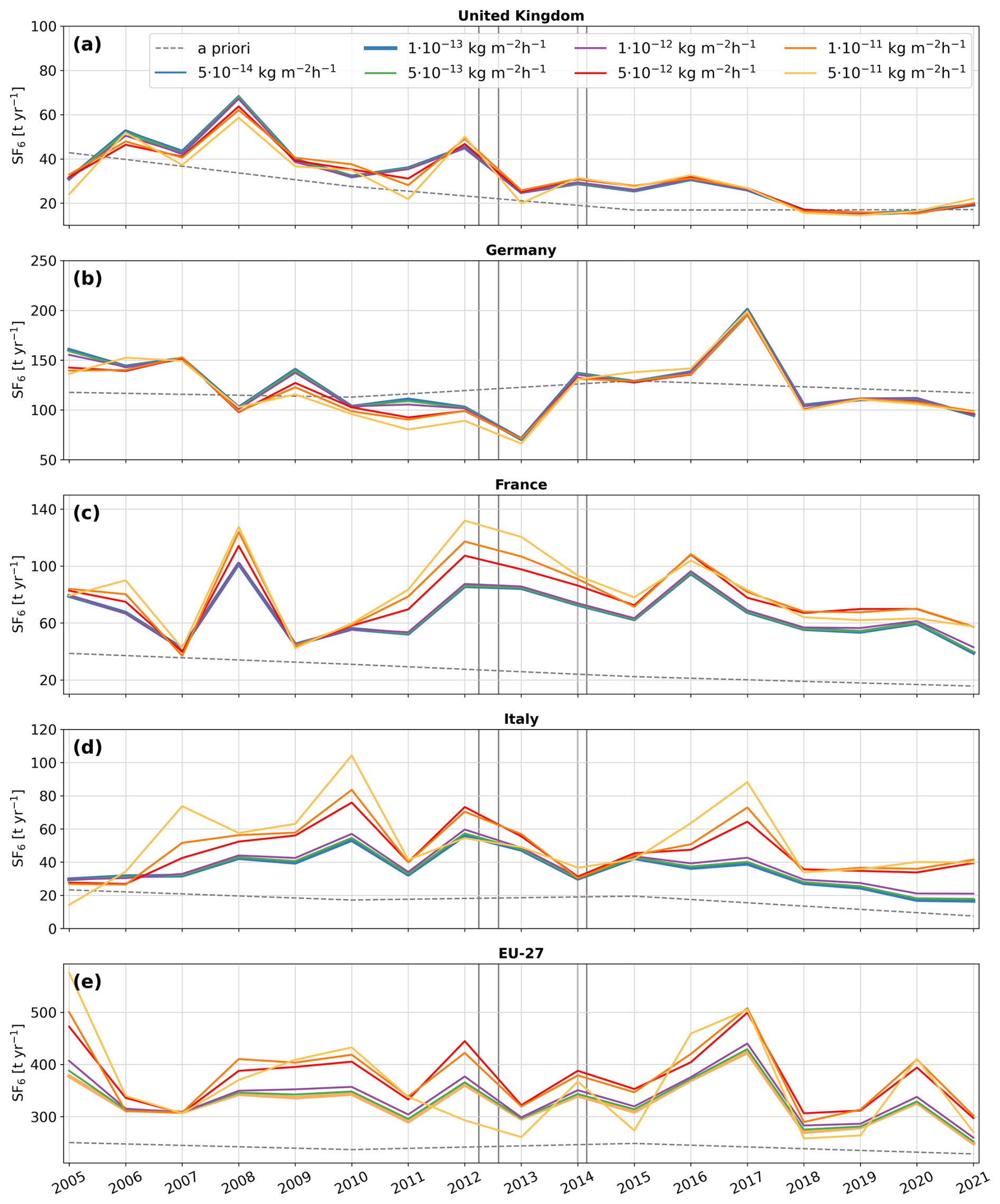
Figure C3 Annual emission time series for (a) the United Kingdom, (b) Germany, (c) France, (d) Italy, and (e) the EU-27, testing different minimal a priori emission uncertainty values. The colored solid lines (dark blue: $\mathrm{5}\times {\mathrm{10}}^{-\mathrm{14}}$, blue: $\mathrm{1}\times {\mathrm{10}}^{-\mathrm{13}}$ , green: $\mathrm{5}\times {\mathrm{10}}^{-\mathrm{13}}$, purple: $\mathrm{1}\times {\mathrm{10}}^{-\mathrm{12}}$, red: $\mathrm{5}\times {\mathrm{10}}^{-\mathrm{12}}$, orange: $\mathrm{1}\times {\mathrm{10}}^{-\mathrm{11}}$, and light orange: $\mathrm{5}\times {\mathrm{10}}^{-\mathrm{11}}\mathrm{kg}{\mathrm{m}}^{-\mathrm{2}}{\mathrm{h}}^{-\mathrm{1}}$) represent the a posteriori emissions derived using the different settings and the gray dashed line shows the a priori emissions.

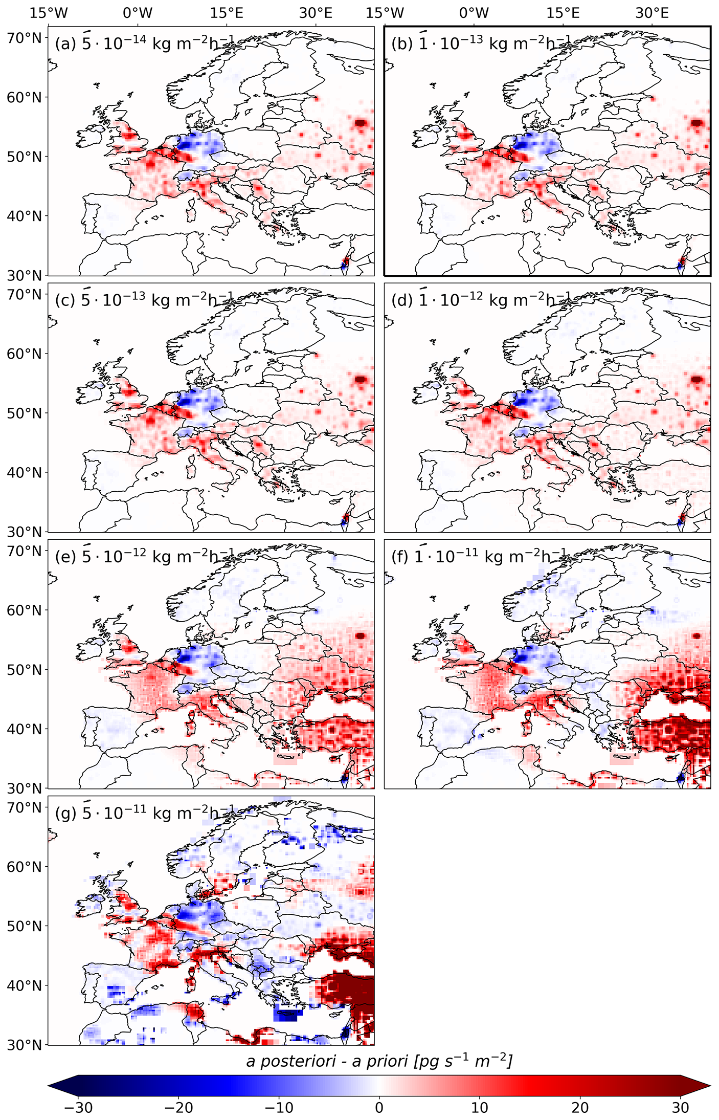
Figure C4 Inversion increments (a posteriori–a priori) for the year 2012, shown for different tested minimal a priori emission uncertainty values (a) $\mathrm{5}\times {\mathrm{10}}^{-\mathrm{14}}\mathrm{kg}{\mathrm{m}}^{-\mathrm{2}}{\mathrm{h}}^{-\mathrm{1}}$, (b) $\mathrm{1}\times {\mathrm{10}}^{-\mathrm{13}}\mathrm{kg}{\mathrm{m}}^{-\mathrm{2}}{\mathrm{h}}^{-\mathrm{1}}$, (c) $\mathrm{5}\times {\mathrm{10}}^{-\mathrm{13}}\mathrm{kg}{\mathrm{m}}^{-\mathrm{2}}{\mathrm{h}}^{-\mathrm{1}}$, (d) $\mathrm{1}\times {\mathrm{10}}^{-\mathrm{12}}\mathrm{kg}{\mathrm{m}}^{-\mathrm{2}}{\mathrm{h}}^{-\mathrm{1}}$, (e) $\mathrm{5}\times {\mathrm{10}}^{-\mathrm{12}}\mathrm{kg}{\mathrm{m}}^{-\mathrm{2}}{\mathrm{h}}^{-\mathrm{1}}$, (f) $\mathrm{1}\times {\mathrm{10}}^{-\mathrm{11}}\mathrm{kg}{\mathrm{m}}^{-\mathrm{2}}{\mathrm{h}}^{-\mathrm{1}}$, and (g) $\mathrm{5}\times {\mathrm{10}}^{-\mathrm{11}}\mathrm{kg}{\mathrm{m}}^{-\mathrm{2}}{\mathrm{h}}^{-\mathrm{1}}$).

Appendix D: Sensitivity to the spatial correlation of the a priori emission uncertainty

FLEXINVERT+ uses an exponential decay function to account for spatial emission uncertainty correlations. We test various spatial scale lengths of 50, 100, 250, 500, 1000 km, as well as a configuration without any spatial correlation. Figure D1 presents the emission time series for these tests. As the correlation length increases, the observational information influences a larger number of emission grid cells, causing the aggregated a posteriori emissions to deviate more from their a priori values. With high correlation lengths, the algorithm’s ability to capture the spatial variability of the emissions is limited. Conversely, if the correlation length is very small, there will be insufficient observational constraint on the emissions. As a consequence, the number of grid cells with substantial inversion increments increases with growing correlation length (see Fig. D2, increments averaged over the study period). At the same time, the modeled error reduction substantially increases (see Fig. D3, error reduction shown for the year 2012). However, this should not be interpreted as an indication of a superior inversion quality. It reflects the broader spatial distribution of observational information rather than an actual improvement in the ability of the inversion to constrain emissions. Our findings align closely with Thompson et al. (2011), who observed a similar error reduction trend when testing correlation lengths between 50 and 2000 km in a European N₂O inversion. Our tests further show that in the absence of spatial correlation, the inversions can yield substantial negative emissions at the grid-cell level (down to$-\mathrm{21}\mathrm{pg}{\mathrm{m}}^{-\mathrm{2}}{\mathrm{s}}^{-\mathrm{1}}$). Such values are unphysical and indicate that the problem is poorly constrained. In contrast, imposing large correlation lengths of 500 and 1000 km slightly reduces the agreement between observed and posterior mole fractions (see Tables S9 and S10), as the imposed correlation limits the inversion's ability to resolve regional emission patterns. Across all investigated regions (Fig. D1), we observe that after 2012, inversion results become less sensitive to the choice of correlation length, especially in Germany (Fig. D1b) and the UK (Fig. D1a), where error reduction is highest (Fig. D3) and inversion results show remarkable stability. In France (Fig. D1c) and Italy (Fig. D1d), the error reduction is smaller and a posteriori emissions remain generally more sensitive to the correlation length. For the aggregated EU-27 emissions (Fig. D1e), results are highly sensitive to the chosen spatial correlation length, though they also stabilize after 2012. Notably, results for correlation lengths of 50, 100, and 250 km are relatively close, while values of 500 km, 1000 km, and no correlation show great deviations in case of the aggregated EU-27 emissions.

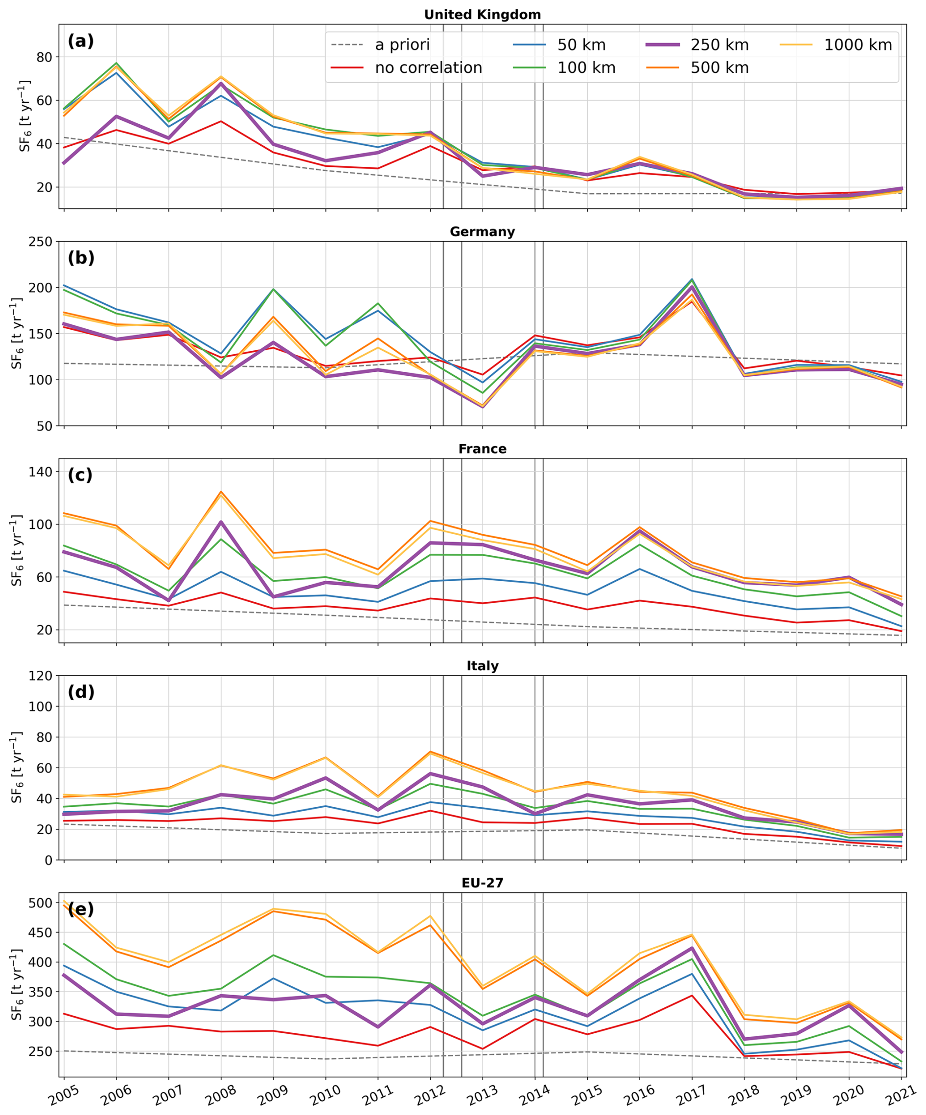
Figure D1 Annual emission time series for (a) the United Kingdom, (b) Germany, (c) France, (d) Italy, and (e) the EU-27, testing different spatial scale lengths for the a priori emission uncertainty correlation. The colored solid lines (blue: 50 km, green: 100 km, purple: 250 km, orange: 500 km, light orange: 1000 km, and red: no correlation) represent the a posteriori emissions derived using the different settings and the gray dashed line shows the a priori emissions. The vertical gray lines indicate the times when additional observational data from the expansion of the UK network became available.

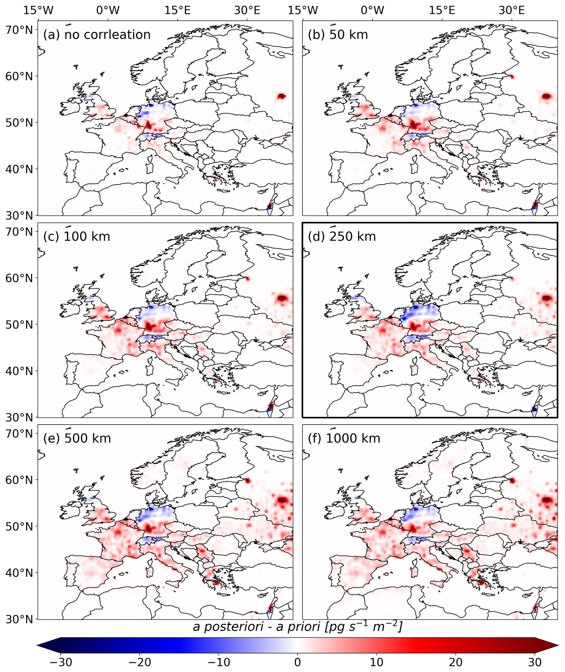
Figure D2 Inversion increments (a posteriori–a priori) averaged over the study period (2005–2021), shown for different spatial scale lengths for the a priori emission uncertainty correlation: (a) no correlation, (b) 50 km, (c) 100,km, (d) 250 km, (e) 500 km, and (f) 1000 km.

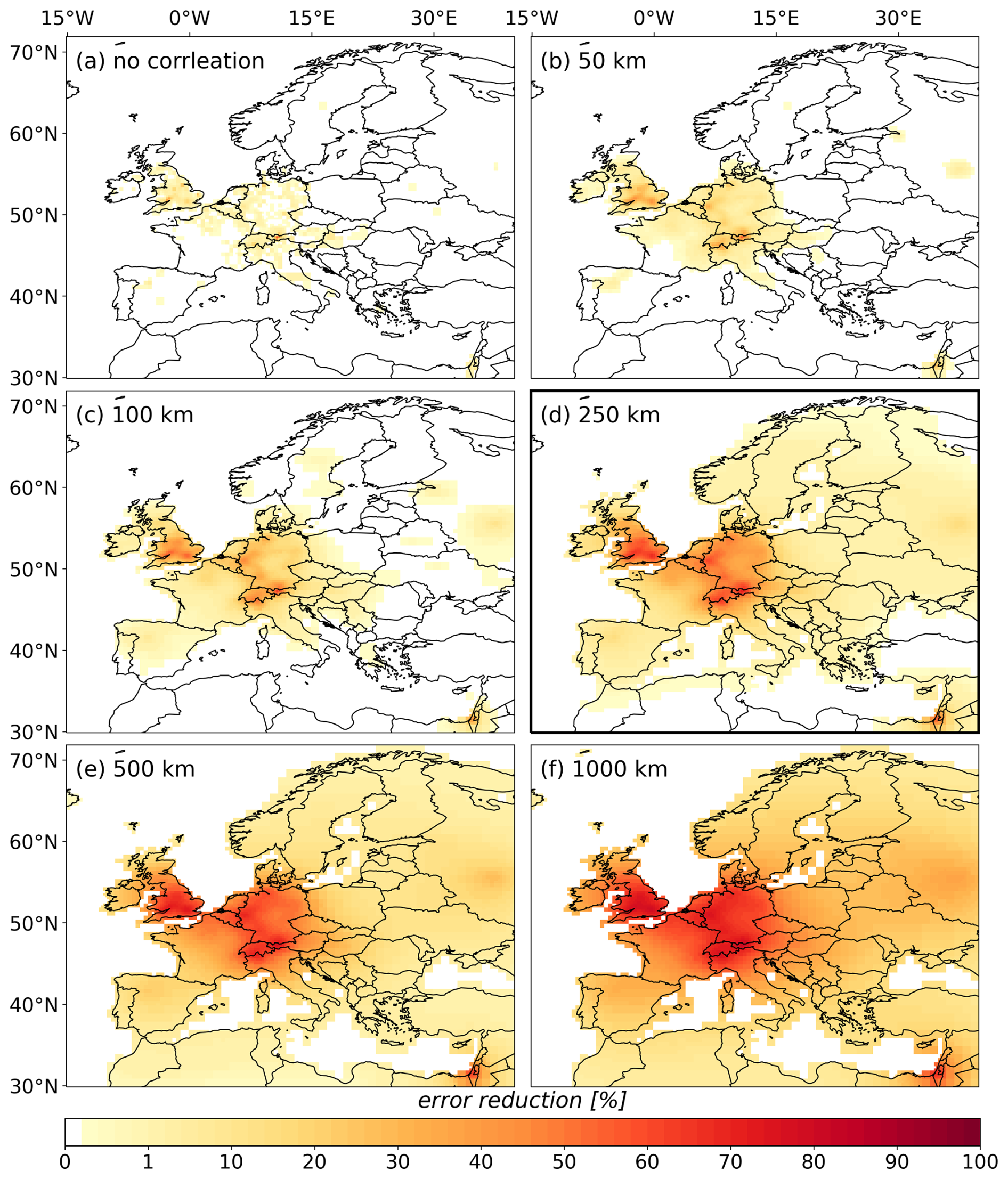
Figure D3 Error reduction for the year 2012, shown for different spatial scale lengths for the a priori emission uncertainty correlation: (a) no correlation, (b) 50 km, (c) 100 km, (d) 250 km, (e) 500 km, and (f) 1000 km.

Appendix E: Sensitivity to the observation datasets

We perform tests using subsets of the global observation dataset: (1) the entire global dataset, (2) the global dataset excluding mountain stations, (3) the global dataset selecting night observations (00:00–06:00) at mountain stations and afternoon observations (12:00–18:00) at other sites, (4) the global dataset using exclusively high-frequency surface observations, (5) the European dataset, a subset of the global dataset (see Sect. 2.1), (6) the European dataset excluding mountain stations, (7) the European dataset selecting night observations at mountain stations and afternoon observations at other sites, and (8) the European dataset using exclusively high-frequency surface observations. Figure E1 presents the emission time series using these datasets.

For the UK, Germany, France and Italy, the choice between the global and European datasets has a small impact on the inversion results; however, for the aggregated EU-27 emissions, differences can be pronounced. This indicates that distant observations have little influence on emissions in countries that are well observed, but can affect emissions in areas that are less well covered. Excluding observations from mountain stations (Fig. E1, red lines) has a minimal impact on the UK emissions (Fig. E1a) and also shows a limited effect in France (Fig. E1c) after 2008. In Germany (Fig. E1b) and the EU-27 (Fig. E1e) the exclusion of mountain stations can lead to notable differences in certain years, while for Italian emissions (Fig. E1d), the impact can be substantial, such as in 2016. Figure E2 shows the 2016 inversion increments, illustrating how the exclusion of the mountain stations (Fig. E2b, f) such as JFJ, ZSF, and CMN, leads to large positive increments in Switzerland and nearby areas (including North Italy), as the observational coverage of this region is drastically reduced. We assume that the limited observational coverage causes the region to be influenced by the high emission increments in southwestern Germany. Selecting only afternoon/night observations (Fig. E1, green lines) generally results in posterior emissions closer to the prior values due to reduced number of available observations. Similarly, the inversion increments (Fig. E2c, g) are attenuated, however, the patterns of emission increments remain rather similar. Excluding flask measurements and data from moving platforms affects early study years (e.g. emissions the UK in Fig. E1a, purple lines), but as the observational coverage with on-line measurement stations increases, the impact of these additional measurements becomes negligible. Similar to the other sensitivity tests, we observe that the sensitivity to the used datasets decreases over the study period, however, 2016 and 2017 stand out as exceptions, likely due to the exceptionally high emissions in southwestern Germany during these years.

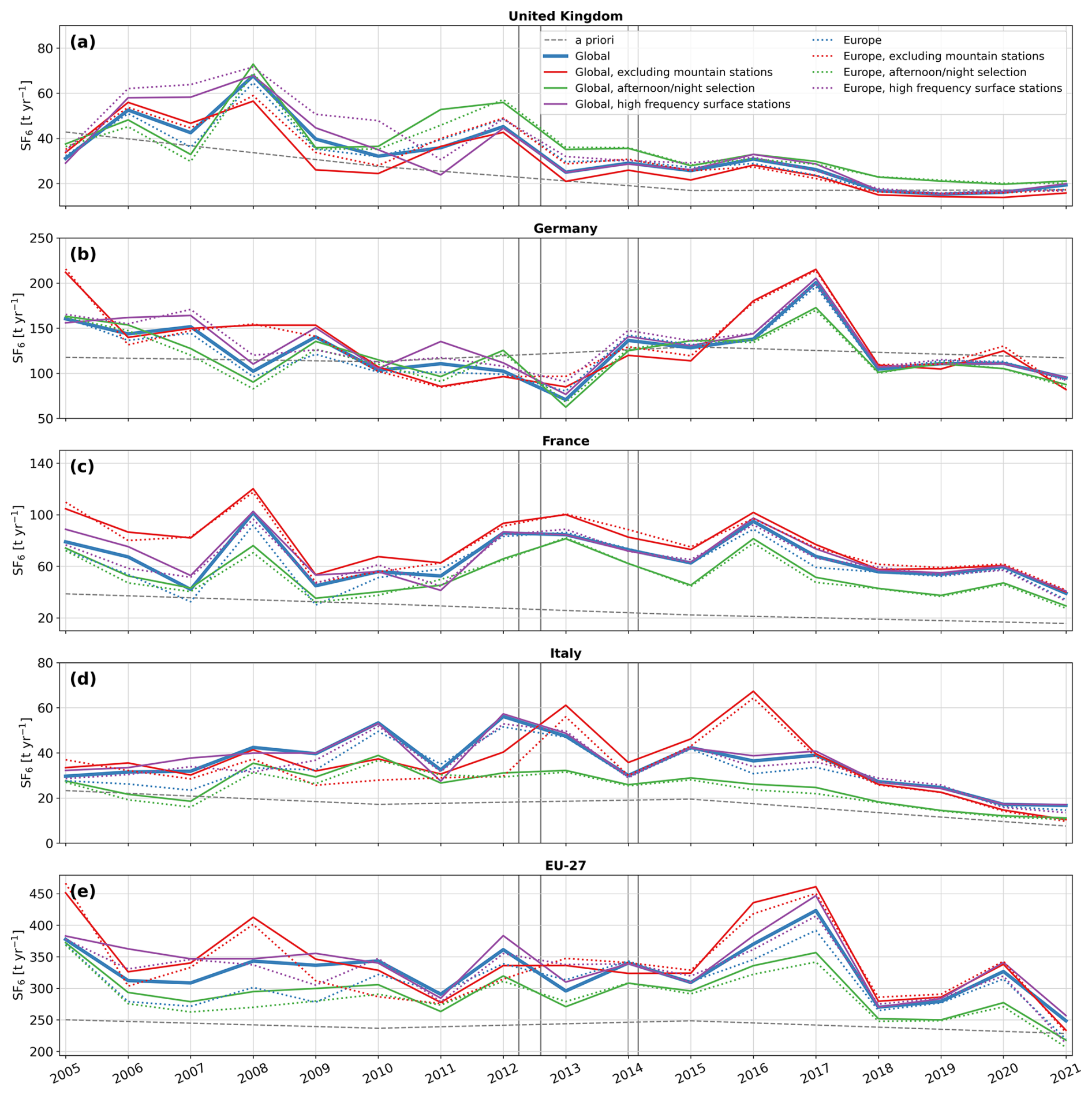
Figure E1 Annual emission time series for (a) the United Kingdom, (b) Germany, (c) France, (d) Italy, and (e) the EU-27, testing different subsets of the observation dataset. The colored lines (solid blue: the full global dataset, solid red: the global dataset excluding mountain stations, solid green: the global dataset selecting night observations at mountain stations and afternoon observations at other sites, solid purple: the global dataset using exclusively high-frequency surface observations, dotted blue: the European dataset, a subset of the global dataset focused on observations in and around Europe, dotted red: the European dataset excluding mountain stations, dotted green: the European dataset selecting night observations at mountain stations and afternoon observations at other sites, dotted purple: the European dataset using exclusively high-frequency surface observations) represent the a posteriori emissions derived using the different settings and the gray dashed line shows the a priori emissions. The vertical gray lines indicate the times when additional observational data from the expansion of the UK network became available.

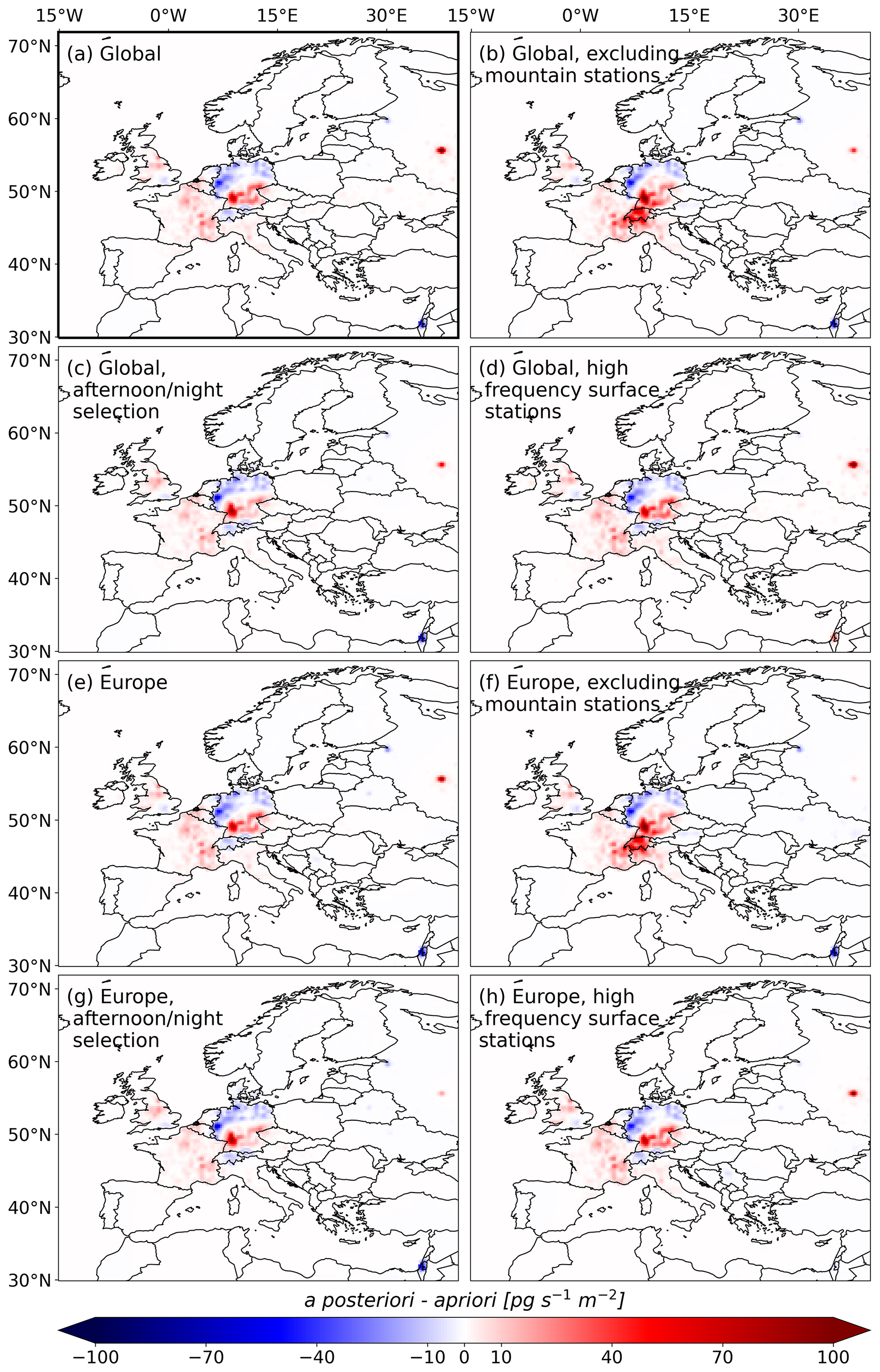
Figure E2 Inversion increments (a posteriori–a priori) for the year 2016, shown for different observation datasets: (a) the full global dataset, (b) the global dataset excluding mountain stations, (c) the global dataset selecting night/afternoon observations, (d) the global dataset using exclusively high-frequency surface observations, (e) the European dataset, a subset of the global dataset focused on observations in and around Europe, (f) the European dataset excluding mountain stations, (g) the European dataset selecting night/afternoon observations (h) the European dataset using exclusively high-frequency surface observations.

Appendix F: Sensitivity to the observation uncertainty

We explore multiple configurations for the observation uncertainty, testing constant values of 0.02, 0.04, 0.06, 0.08, and 0.1 ppt. Additionally, we use two approaches where we (i) base the observation error on the RMSE between a priori modeled and observed values, averaged by station, and (ii) estimate the model error from the standard deviation of the a posteriori error distribution at each station, using initial inversion runs. Figure F1 presents the emission time series of these tests. As observation uncertainty increases, the observational constraint weakens, causing the a posteriori emissions to follow more closely their a priori values. The two approaches that account for spatial variability in the model uncertainty generally fall within the range of constant-error settings, although they show a slightly different pattern for some periods. The inversion results show very low sensitivity to the observation uncertainty in the UK and Germany, especially after 2012 when results are extremely stable. For France, Italy, and the EU-27, the sensitivity to the observation uncertainty also declines after 2012. The reduced chi-squared values averaged over the study period were 3.65, 1.50, 0.87, 0.57, and 0.41 for assumed observation errors of 0.02, 0.04, 0.06, 0.08, and 0.10 ppt, respectively. These results suggest that an observation error of about 0.06 ppt provides the most consistent fit, while 0.02 ppt underestimates and 0.10 ppt overestimates the uncertainties. Note at this point that the smallest error setting of 0.02 ppt (red) shows the greatest deviation from the other tests. The chi-squared values related to the spatial varying uncertainties were 0.80 (standard deviation, a posteriori distribution), and 0.31 (RMSE, a priori distribution). Indeed, using the RMSE of the a priori distribution is expected to be an overestimation, as it also reflects systematic mismatches and biases in the a priori emissions rather than purely observational and transport model uncertainty.

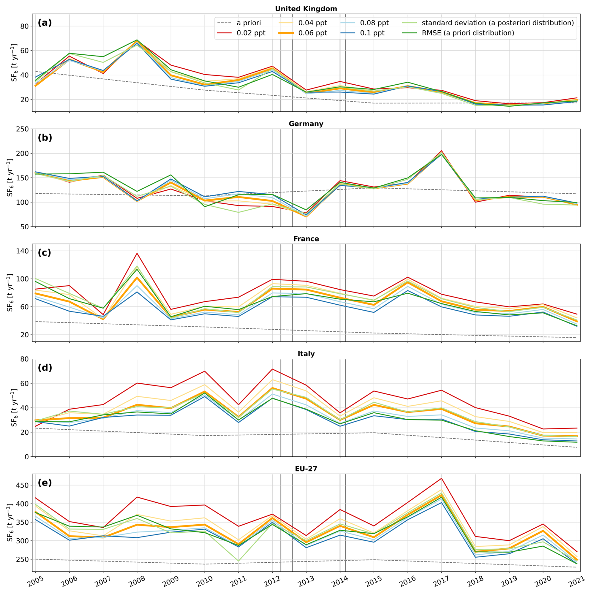
Figure F1 Annual emission time series for (a) the United Kingdom, (b) Germany, (c) France, (d) Italy, and (e) the EU-27, testing various observation error settings. The colored solid lines (red: 0.02 ppt, orange: 0.04 ppt, light orange: 0.06 ppt, light blue: 0.08 ppt, blue: 0.1 ppt, light green: standard deviation of the a posteriori distribution, green: RMSE between a priori modeled and observed values) represent the a posteriori emissions derived using the different settings and the gray dashed line shows the a priori emissions. The vertical gray lines indicate the times when additional observational data from the expansion of the UK network became available.

Appendix G: Sensitivity to the baseline optimization

FLEXINVERT+ includes an option for baseline optimization, where spatially aggregated contributions are adjusted on a coarse grid. We test different coarse grid resolutions by dividing the global field into 8, 4, and 2 latitude bands, with northern boundaries at [−60°, −30°, −15°, 0°, 15°, 30°, 60°, 90°], [−30°,0°, 30°, 90°], and [0°, 90°], respectively. In addition, we run inversions where the entire global field is optimized with a single scalar. Figure G1 presents the emission time series for these tests. For all regions studied, we find that optimizing the baseline using 2, 4, or 8 latitudinal bands has minimal impact on the results. However, optimizing the entire field in a single global grid cell results in significantly higher a posteriori emissions, particularly before 2012, especially evident for the EU-27 emissions (Fig. G1e). This trend is also evident in the inversion increments (Fig. G2), where the positive increments are larger, and the negative increments are less pronounced when optimizing the whole field (Fig. G2a). These results can be linked to the large inter-hemispheric gradient in atmospheric SF₆ mole fractions. Potential biases in the modeled SF₆ mole fraction fields likely differ between the Southern and Northern Hemispheres, making a single optimization factor insufficient to represent both regions accurately. However, as the observational coverage increases, the sensitivity to the spatial resolution of the baseline drastically decreases and inversion results become extremely stable for all tested regions.

We also test different temporal baseline optimization intervals of 15, 30, 45, and 60 d, with inversion results shown in Fig. G3. The a posteriori emissions are only minimally sensitive to the choice of the temporal interval between 15 and 60 d. Although small differences occasionally appear in certain years and regions, the overall inversion results remain highly stable. Furthermore, we test various baseline uncertainty values set to 0.0001, 0.0003, 0.0005, 0.0007, 0.0009, 0.001, 0.01, 0.1, and 1 ppt and run an inversion without any baseline optimization. The resulting a posteriori emission time series are shown in Fig. G4. The baseline optimization consistently reduces the a posteriori emissions across all regions, indicating that the optimization tends to shift the a posteriori baseline to higher values. At a baseline uncertainty of 0.0001 ppt, the changes in a posteriori emissions are minimal. However, increasing the uncertainty to 0.0003 ppt produces a notable decrease in emissions. Further increases in the uncertainty continue to lower the a posteriori emissions, though the effect diminishes with each step, converging toward stable results between 0.01 and 0.1 ppt. Increasing the baseline uncertainty up to 0.01 ppt also improves the bias between a posteriori modeled and observed mole fractions while higher uncertainties yield the same results (see Tables S11–S13). Figure G5 presents the inversion increments for uncertainty values between 0.0001 and 0.01 ppt, as well as for the case without optimization. Consistent with Fig. G4, we observe a decrease in increments with increasing baseline uncertainty. As observed in other sensitivity studies, the sensitivity to baseline optimization decreases significantly over the course of the study period, with results stabilizing toward the end for all tested regions.

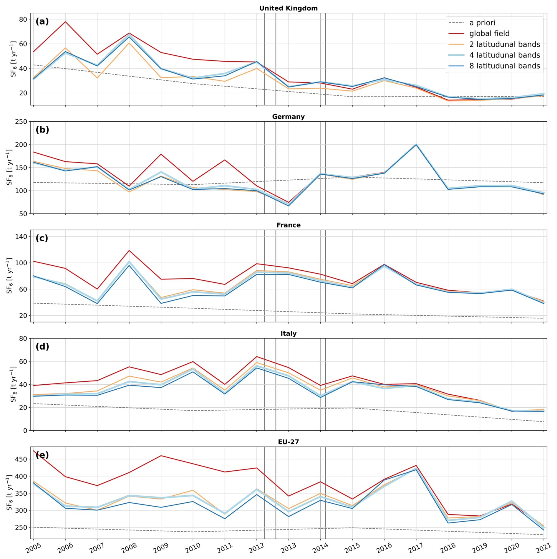
Figure G1 Annual emission time series for (a) the United Kingdom, (b) Germany, (c) France, (d) Italy, and (e) the EU-27, testing various spatial resolutions of aggregated baseline contributions for the baseline optimization. The colored solid lines represent the a posteriori emissions derived when optimizing the baseline, regarding the different spatial resolutions (red: the whole global field, orange: 2 latitudunal bands, light blue: 4 latitudunal bands, and blue: 8 latitudunal bands). The gray dashed line shows the a priori emissions. The vertical gray lines indicate the times when additional observational data from the expansion of the UK network became available.

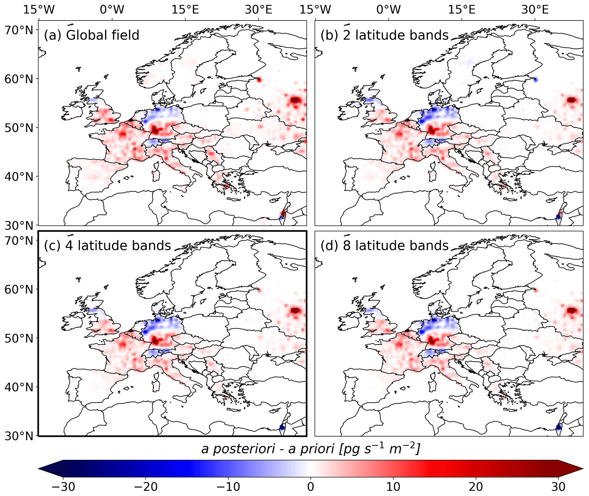
Figure G2 Inversion increments (a posteriori–a priori) averaged over the study period (2005–2021), shown for various spatial resolutions of aggregated baseline contributions for the baseline optimization: (a) the whole field, (b) 2 latitudinal bands, (c) 4 latitudinal bands, and (d) 8 latitudinal bands.

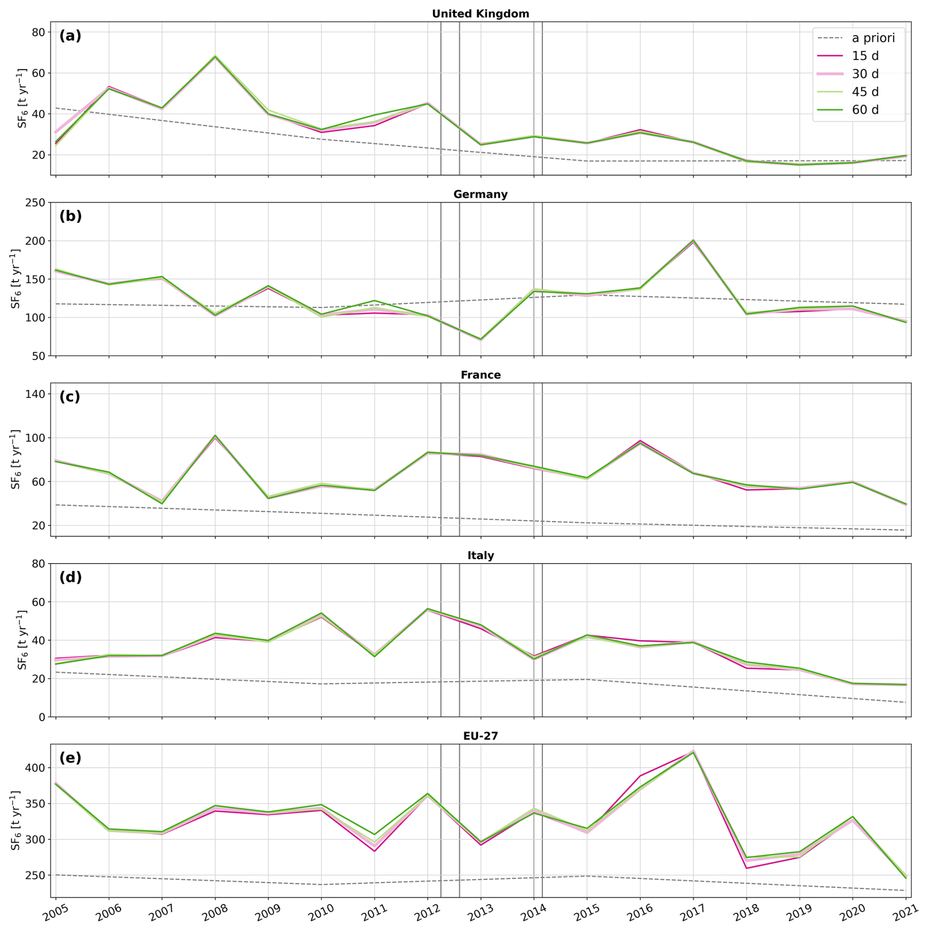
Figure G3 Annual emission time series for (a) the United Kingdom, (b) Germany, (c) France, (d) Italy, and (e) the EU-27, testing different temporal baseline optimization intervals. The colored solid lines (pink: 15 d, orange: 30 d, light green: 45 d, and green: 60 d) represent the a posteriori emissions. The gray dashed line shows the a priori emissions. The vertical gray lines indicate the times when additional observational data from the expansion of the UK network became available.

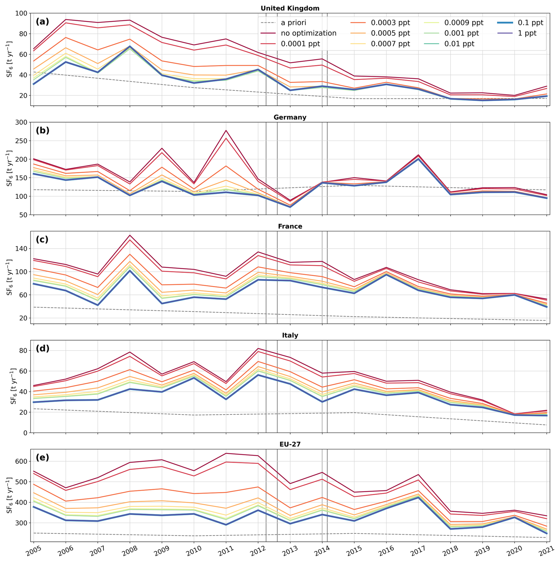
Figure G4 Annual emission time series for (a) the United Kingdom, (b) Germany, (c) France, (d) Italy, and (e) the EU-27, testing baseline uncertainty values. The colored solid lines represent the a posteriori emissions (dark red: no optimization , red: 0.0001 ppt, dark orange: 0.0003 ppt, orange: 0.0005 ppt, light orange: 0.0007 ppt, light green 0.0009 ppt, green 0.001 ppt, dark green 0.01 ppt, light blue 0.1 ppt, and blue: 1 ppt). These tests refer to a baseline optimization using 4 latitudinal bands and a 30 d temporal time window. The gray dashed line shows the a priori emissions. The vertical gray lines indicate the times when additional observational data from the expansion of the UK network became available.

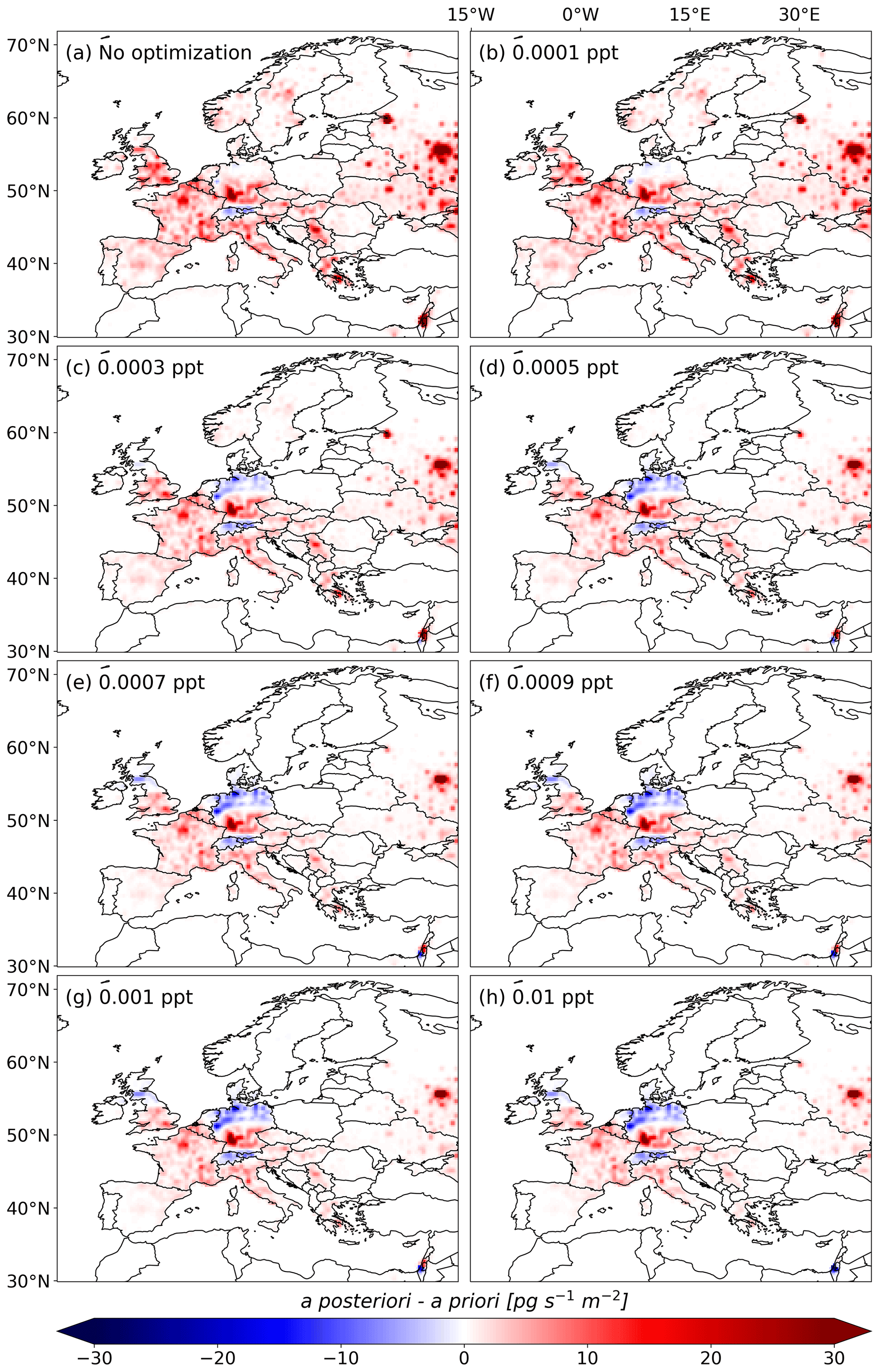
Figure G5 Inversion increments (a posteriori–a priori) averaged over the study period (2005–2021), shown for various baseline uncertainty values: (a) no optimization, (b) 0.0001 ppt (c) 0.0003 ppt, and (d) 0.0005 ppt, (e) 0.0007 ppt, (f) 0.0009 ppt, (g) 0.001 ppt, (h) 0.01 ppt.

Appendix H: Sensitivity to the emission grid

We utilize emission grids with varying cell sizes, created by aggregating cells with low emission contributions based on emission sensitivities and a priori emissions (see details in Thompson and Stohl, 2014). The tested grids include configurations with 588, 744, 1992, 2781, 4248, 5370, and 7229 grid cells, each remaining constant over time. Additionally, we explore three dynamic setups where the grid configuration adjusts annually, with the number of cells ranging from (i) 2781 to 5916, (ii) 3645 to 6599, and (iii) 4151 to 7229. Figure H1 illustrates the emission grid with (a) the highest and (b) the lowest number of grid cells, while Fig. H2 displays the inversion results for all tested grid configurations. The inversion results demonstrate minimal sensitivity to the number of grid cells within the tested range, with only minor differences observed in isolated years and regions.

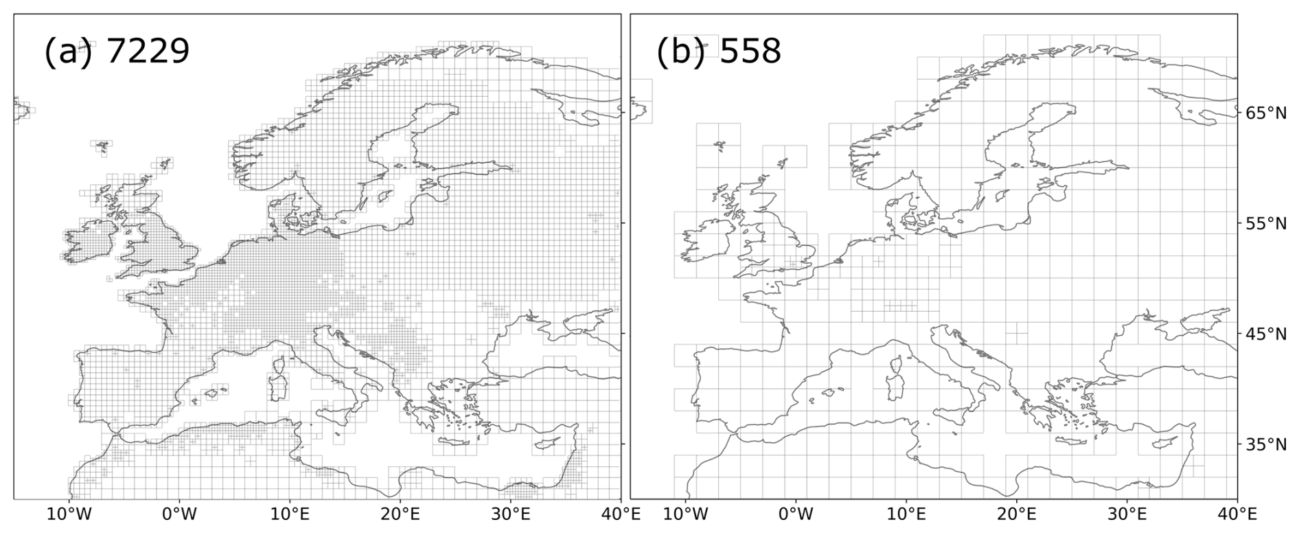
Figure H1 European inversion grid with variable cell sizes, featuring configurations of (a) 7229 and (b) 588 grid cells.

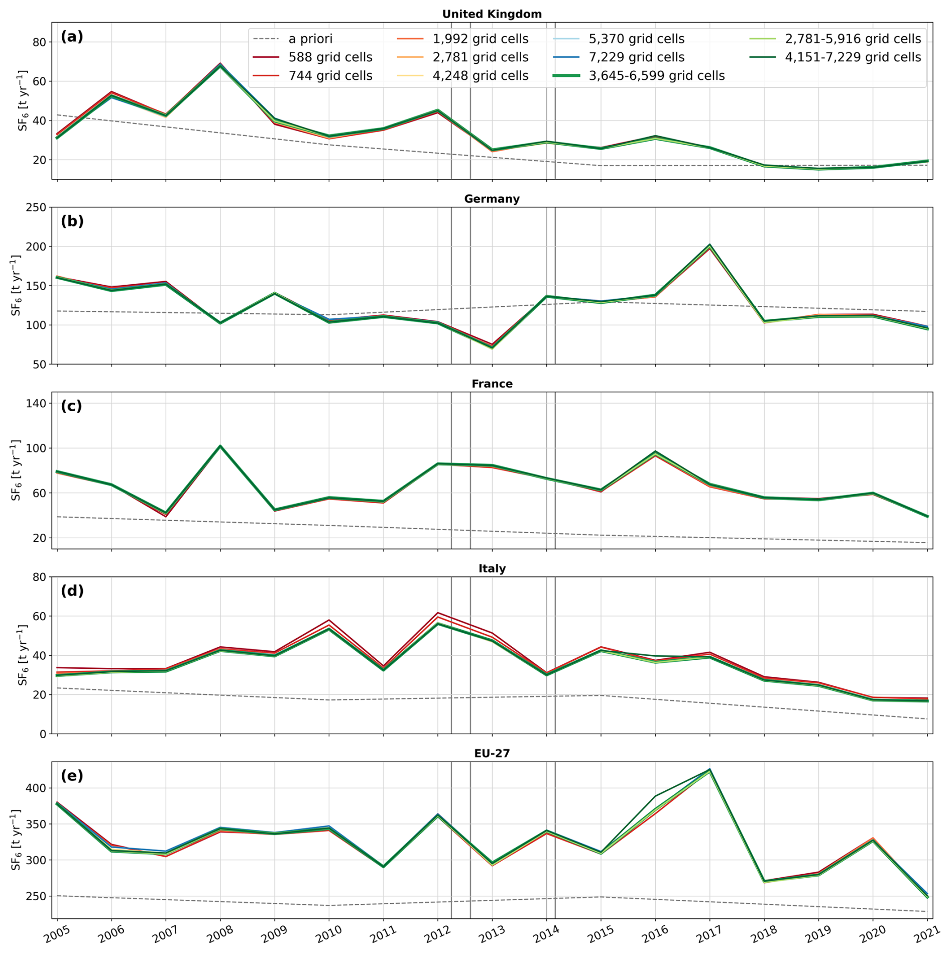
Figure H2 Annual emission time series for (a) the United Kingdom, (b) Germany, (c) France, (d) Italy, and (e) the EU-27, testing various emission grid configurations. The colored solid lines represent the a posteriori emissions (dark red: 588, red: 744 ppt, dark orange: 1992, orange: 2781, light orange: 4248, light blue 5370, blue 7229, light green: 2781–5916, green 3645–6599, and dark green: 4151–7229 grid cells). The gray dashed line shows the a priori emissions. The vertical gray lines indicate the times when additional observational data from the expansion of the UK network became available.

Appendix I: Sensitivity to the whole inversion ensemble

Figure I1 shows the results of all performed inversions, displaying the full set of a posteriori emissions alongside the average across all sensitivity tests. Our results show that sensitivity to the various inversion settings decreases significantly after 2012, aligning with the expansion of the British observation network. This trend is particularly evident in the UK and Germany, where the results become highly stable across all sensitivity tests. Even under unfavorable settings that lead to outliers during periods of limited observational coverage, results remain stable towards the end of the study period.

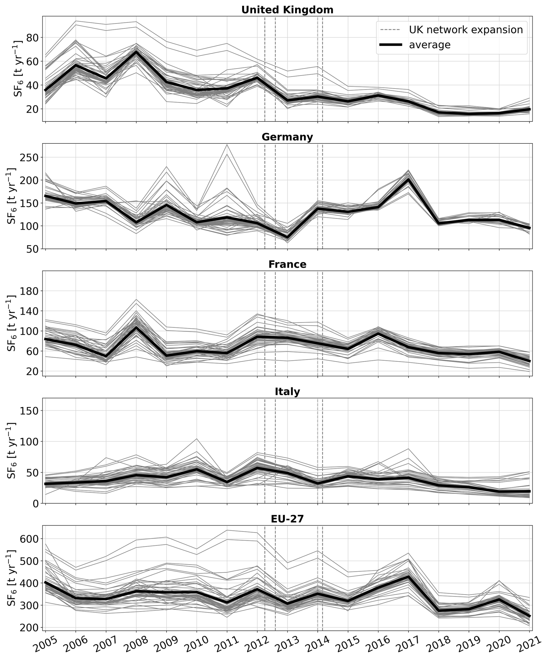
Figure I1 Annual emission time series for (a) the United Kingdom, (b) Germany, (c) France, (d) Italy, and (e) the EU-27. The solid gray lines represent the inversion results of all sensitivity tests and the solid black lines represent the average a posteriori emissions across all performed tests.The vertical dashed gray lines indicate the times when additional observational data from the expansion of the UK network became available.

Appendix J: Selection of parameter ranges

Based on the insights from our sensitivity tests, we defined the final parameter ranges for the inversion ensemble. Compared to the broader ranges explored in the sensitivity tests, these final ranges are narrowed to exclude (i) unlikely values that could lead to extreme or problematic results and (ii) parameters to which the inversion showed negligible sensitivity.

• i.

  A priori emission uncertainty: We adopt a normal distribution with mean 0.5 and standard deviation 0.1. Within this range, the inversion yields reasonable results and reduced chi-squared values close to one (see Appendix C).

• ii.

  Minimal a priori emission value: We adopt a normal distribution with mean $\mathrm{5}\times {\mathrm{10}}^{-\mathrm{13}}\mathrm{kg}{\mathrm{m}}^{-\mathrm{2}}{\mathrm{h}}^{-\mathrm{1}}$ and standard deviation $\mathrm{1}\times {\mathrm{10}}^{-\mathrm{13}}\mathrm{kg}{\mathrm{m}}^{-\mathrm{2}}{\mathrm{h}}^{-\mathrm{1}}$. Values above this range lead to less localized inversion increments that spread over larger areas. This could potentially introduce biases in regions with sparse observational constraints (see Appendix C).

• iii.

  Spatial correlation of a priori emission uncertainty: We adopt a normal distribution with mean 250 km and standard deviation 100 km. This choice represents our best estimate of a compromise between sufficiently constraining emissions and maintaining the inversion’s ability to resolve regional emission patterns (see Appendix D).

• iv.

  Observation uncertainty: We adopt a normal distribution with mean 0.06 ppt and standard deviation 0.01 ppt. Uncertainties within this range yield stable inversion results, while reduced chi-squared values remain close to one (see Appendix F).

• v.

  Baseline optimization: We optimize the baseline in eight latitudinal bands, which improves performance compared to using a single global factor. The baseline uncertainty is set to 0.1 ppt to avoid underestimation, as smaller values (especially <0.01 ppt) can introduce biases. Inversion results were largely insensitive to the choice of baseline optimization time window, for which we therefore adopted a value of 30 d (see Appendix G).

• vi.

  Emission grid: We employ an emission grid of 558 cells, since the sensitivity tests indicated negligible dependence of the results on the grid within the tested configurations (see Appendix H).

• vii.

  A priori and observational datasets: For these inputs, we sample randomly from the datasets described in Sect. 2.3 and 2.1, as there were no objective reasons to restrict their parameter space.