Airborne in situ quantification of methane emissions from oil and gas production in Romania

Production of oil and gas in Romania, one of the largest producers in the European Union (EU), is associated with substantial emissions of methane to the atmosphere and may offer high emission mitigation potential to reach the climate objectives of the EU. However, comprehensive quantification of emissions in this area has been lacking. Here we report top-down emission rate estimates derived from aircraft-based in situ measurements that were carried out with two aircraft during the 2019 ROmanian Methane Emissions from Oil and gas (ROMEO) campaign, supported by simulations with atmospheric models. Estimates from mass balance flights at individual dense production clusters and around larger regions show large variations between the clusters, supporting the important role of individual super-emitters, and possibly show variable operation practices or maintenance states across the production basin. Estimated annual total emissions from the southern Romanian oil and gas (O&G) infrastructure are 227 ± 86 kt CH₄ yr⁻¹, consistent with previously published estimates from ground-based site-level measurements during the same period. The comparison of individual plumes between measurements and atmospheric model simulations was complicated by unfavorable low-wind conditions. Similar correlations between measured and simulated CH₄ enhancements during large-scale raster flights and mass balance flights suggest that the emission factor determined from a limited number of production clusters is representative of the larger regions. We conclude that ground-based and aerial emission rate estimates derived from the ROMEO campaign agree well, and the aircraft observations support the previously suggested large under-reporting of CH₄ emissions from the Romanian O&G industry in 2019 to United Nations Framework Convention on Climate Change (UNFCCC). We also observed large underestimation from O&G emissions in the Emissions Database for Global Atmospheric Research (EDGAR) v7.0 for our domain of study.

1 Introduction

Methane (CH₄) is a potent greenhouse gas with more than 80 times the global warming potential of carbon dioxide (CO₂) over a 20-year time horizon (Szopa et al., 2021). Approximately 60 % of global CH₄ emissions are attributed to human activities, with roughly one-third of them resulting from the oil and gas (O&G) industry (Saunois et al., 2020). Reducing CH₄ emissions from the O&G industry presents an easily accessible and cost-effective mitigation option (United Nations Environment Programme and Climate and Clean Air Coalition, 2021). Given the relatively short lifetime of CH₄ in the atmosphere (≈ 10 years), such measures would lead to substantial climate benefits in both the near- and long-term future (United Nations Environment Programme and Climate and Clean Air Coalition, 2021; Collins et al., 2018). Scenarios that are compatible with the goal of the Paris Agreement (UNFCCC, 2015) to limit global warming to 2 °C, preferentially to 1.5 °C, all include substantial reductions in CH₄, and the current growth in CH₄ is incompatible with reaching this goal (Nisbet et al., 2020).

Improving our understanding of CH₄ emissions from the O&G industry requires comprehensive and accurate emission measurements using a combination of approaches. Several studies, mostly in North America, consistently show that national inventories, which rely on multiplying activity data with generic emission factors, tend to underestimate CH₄ emissions from the O&G industry (Allen et al., 2013; Brandt et al., 2014; Harriss et al., 2015; Johnson et al., 2017; Alvarez et al., 2018; Weller et al., 2020).

CH₄ emissions can be quantified using top-down or bottom-up approaches. Top-down approaches use ambient CH₄ mole fraction measurements from aircraft, tall towers, weather stations, or satellites combined with models to estimate the total CH₄ flux rate at different scales (i.e., site-level to regional- or country-level). These approaches ensure that emissions from all sources are captured. Other techniques, such as the use of ethane (C₂H₆) and the isotopic composition of CH₄ as tracers, can help attribute CH₄ emissions to the O&G industry or to other sectors (Röckmann et al., 2016; Lopez et al., 2017; Mielke-Maday et al., 2019; Maazallahi et al., 2020; Lu et al., 2021; Menoud et al., 2021; Gonzalez Moguel et al., 2022; Fernandez et al., 2022). Bottom-up approaches involve direct measurements of emissions usually at the source or component level, which are then extrapolated to larger scales using statistical methods.

The emission data reported to the United Nations Framework Convention on Climate Change (UNFCCC) for the year 2021 reveal that Romania ranks among the European Union (EU) countries with the highest annual CH₄ emissions from O&G activities, following closely behind Italy and Poland (UNFCCC, 2023a). The International Energy Agency (IEA) estimates that Romania contributes the highest CH₄ emissions from the O&G industry among the 27 EU countries (IEA, 2023). In light of the recent provisional agreement regarding EU methane regulations, which impose new requirements on the O&G industry for measuring, reporting, and mitigating CH₄ emissions (European-Commission, 2023), there is an urgent need to understand the extent and magnitude of emissions. This is particularly relevant for countries like Romania, where emissions are substantial but understudied and addressing them is crucial for achieving EU climate objectives.

The ROMEO (ROmanian Methane Emissions from Oil and gas) project was designed to provide independent scientific-measurement-based CH₄ emission estimates for the O&G producing regions in Romania (Stavropoulou et al., 2023). The first phase of the ROMEO campaign took place in October 2019, covering large production areas in southern Romania that are mostly associated with oil production. The second phase happened in the following year and focused on the gas production region in the Transylvanian Basin, north of the mountain range. Numerous measurement techniques using a variety of instruments were deployed on board ground-based and airborne measurement platforms. The data collected by vehicles and uncrewed aerial vehicles (UAVs) during the ROMEO campaign have already been evaluated separately in previous studies (Stavropoulou et al., 2023; Delre et al., 2022; Korbeń et al., 2022). Additionally, Menoud et al. (2022) investigated the isotopic signature of CH₄ emissions from the sites visited during the ROMEO campaign, contributing to insights into the reservoir characteristics.

In this study, we present top-down CH₄ emission estimates derived from aircraft measurements of individual facilities, facility clusters, and extended regions during the ROMEO campaign. The measurements were performed by two research aircraft, and we used two mesoscale atmospheric chemistry and transport models to simulate atmospheric composition and transport over Romania.

2 Materials and methods

2.1 Clusters and regions

Information about O&G activities including locations, production asset types, and status and age of the facilities was received from the largest operator in the region. This information covers the majority of the sites in the survey region, although other, smaller operators are also present. The distribution of O&G production infrastructure in Romania is heterogeneous, with a high density of production sites concentrated above the subsurface fossil fuel reservoirs. Therefore, we first grouped the installations into 40 clusters (Cs) and regions (Rs) (i.e., the aggregation of several production clusters) (Fig. 1). Both production clusters and regions were targets for the quantification approaches in the ROMEO campaign. Clusters are relatively small areas, usually a few square kilometers to 20 km², with a high density of O&G production sites. To derive basin-scale emission rates from aircraft measurements, the Romanian plain was further divided into larger regions of roughly 50 × 50 km², which contain the clusters and are suitable for aircraft mass balance and raster flights.

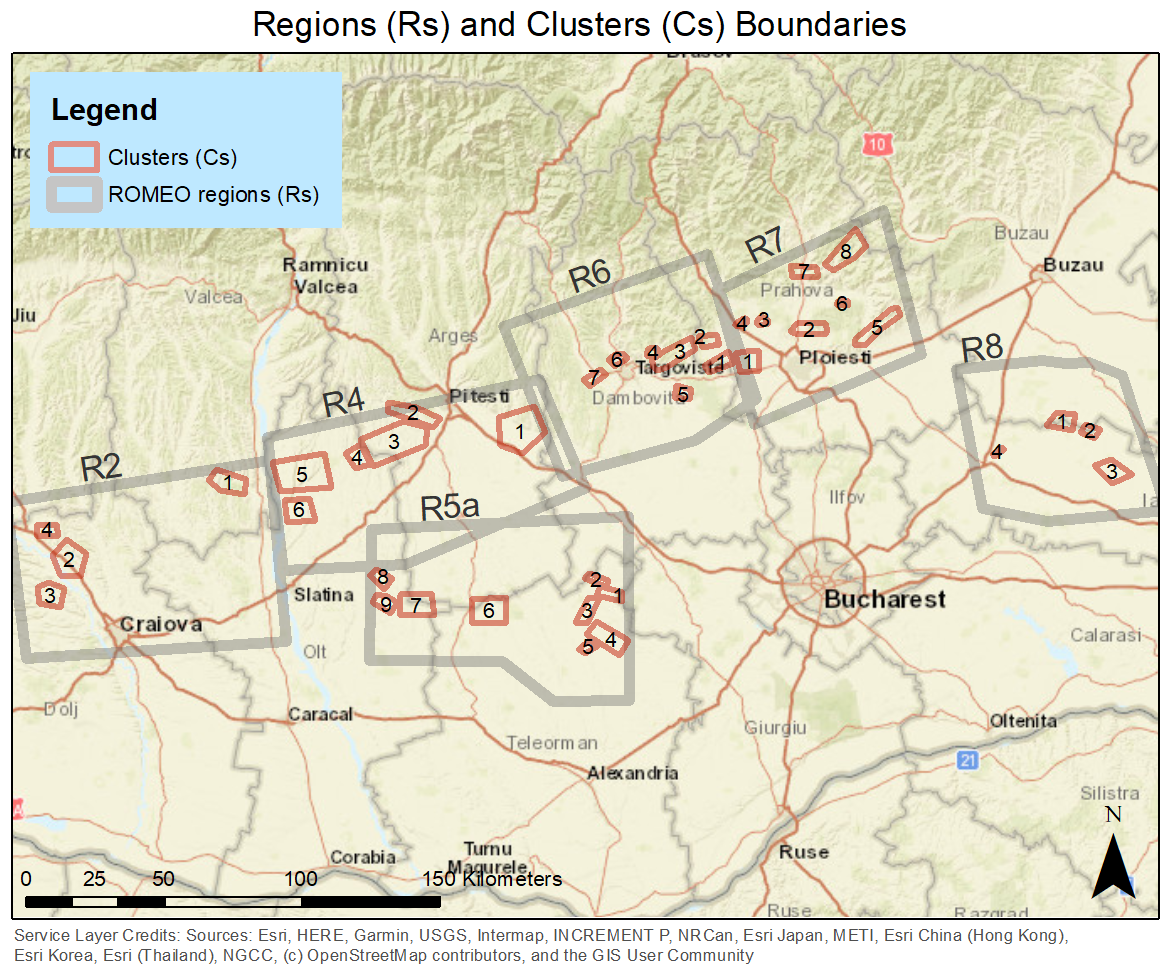
Figure 1 Regions (gray polygons) and clusters (red polygons) that were targeted during the ROMEO 2019 campaign; circular or raster flights were performed within or around these boundaries.

2.2 Aircraft-based in situ measurements

Two aircraft were deployed during the ROMEO 2019 campaign: a BN2 aircraft operated by the National Institute for Aerospace Research “Elie Carafoli” (INCAS) and a two-seater Mooney aircraft operated by Scientific Aviation (SA) Inc. On the Mooney aircraft, in situ measurements of CH₄, C₂H₆, carbon dioxide (CO₂), wind speed and direction, and relative humidity were continuously logged at 1 Hz frequency. C₂H₆ and CO₂ were measured with AERIS Pico Mobile LDS and Picarro G2301-f instruments, and both instruments measured CH₄ individually. On the BN2 aircraft, CH₄, CO₂, and carbon monoxide (CO) were measured at about 0.3 Hz frequency using a G2401 analyzer (Picarro Inc).

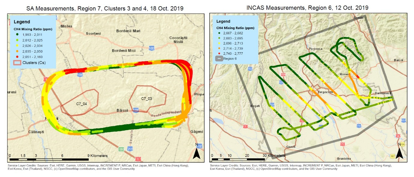
Figure 2 Examples of a mass balance flight with the south wind from measurements (a) and a raster flight with an east–east–north wind from simulations (b) during the ROMEO 2019 campaign. The mass balance flight circled around two production clusters located in close proximity, and the raster flight covers a larger region. The color scale represents the CH₄ mole fraction.

Two sets of flight patterns were performed: mass balance flights circling around target areas (Fig. 2, left) and raster flights scanning the areas at a pre-selected observation density (Fig. 2, right). During the 18 individual mass balance flights with the SA aircraft, the target emission locations were circled at different altitudes to map the extent of the emission plume(s), both vertically and horizontally. The emission rates were then calculated from the measurements of the CH₄ mole fraction and wind speed and direction in the mass balance approach (see below). The BN2 aircraft was used to map possible emission sources over more extended areas. The lack of wind measurements from this aircraft precludes direct emission quantification using the mass balance approach. These extended areas were surveyed in raster patterns perpendicular to the prevailing wind (Fig. 2b). In addition to the identification of larger sources, these measurements are also used to derive indirect emission rate estimates by comparison to model simulations (see below).

2.3 Model simulations

In order to support the emission quantification from the aircraft measurements, we simulated atmospheric composition and transport over Romania using two numerical mesoscale atmospheric chemistry and transport models: COSMO-GHG (Consortium for Small-scale Modeling – Greenhouse Gases) operated by the Swiss Federal Laboratories for Materials Science and Technology (EMPA) and MECO(n) (MESSy-fied ECHAM and COSMO models nested n times) operated by the German Aerospace Center (DLR). COSMO-GHG is based on the regional numerical weather prediction and climate model COSMO-CLM (Baldauf et al., 2011) and includes the greenhouse gas (GHG) extension (Jähn et al., 2020; Brunner et al., 2019) for the simulation of (nearly) passive trace gases such as CH₄. MECO(n) features an online coupling of the global chemistry–climate model EMAC (ECHAM–MESSy Atmospheric Chemistry) with the regional chemistry–climate model COSMO-CLM/MESSy (Kerkweg and Jöckel, 2012). The COSMO-GHG simulations were nudged to the hourly wind data from the ERA5 reanalysis product of the European Centre for Medium-Range Weather Forecasts (ECMWF) (Hersbach et al., 2023). In MECO(n) the global model (EMAC) was nudged by Newtonian relaxation towards the operational analysis data from ECMWF (see Nickl et al., 2020, for more details).

These two models were used to simulate the evolution of the CH₄ mole fraction arising from emissions from active O&G assets, including individual wells and larger facilities in time and space. To set up the model simulations, each site was assigned an emission rate of 1 g s⁻¹ (3.6 kg h⁻¹). For COSMO-GHG, the model resolution was 2 × 2 km², and the meteorological and compositional boundary conditions were provided from global-scale modeling results obtained with the ECMWF-CAMS system. The MECO(n=3) setup comprised four model instances (see Klausner et al., 2020, for a detailed description of a similar model setup). The first is the global model instance EMAC with a resolution of T42L90MA (corresponding to around 280 km spatial resolution). In the global model, three COSMO-CLM/MESSy instances were nested online with approx. 50 km resolution, approx. 7 km resolution, and the same 2 × 2 km domain as was applied to COSMO-GHG. In the MECO(3) setup applied, we used a parameterized chemistry of methane (Winterstein and Jöckel, 2021) with monthly mean OH fields from previous simulations with comprehensive interactive chemistry. In the first, second, and third MECO(3) model instances, we prescribed all anthropogenic and natural emissions of methane in order to achieve realistic boundary conditions of methane for the finest-resolved instance. In this instance the emissions were used as described below. The model outputs provide atmospheric CH₄ mole fraction fields as well as meteorological parameters at a temporal resolution of 20 min (COSMO-GHG) and 1 h (MECO(3)). For MECO(3), only the results of the finest instance are considered here for further analysis. To be able to geo-attribute emissions to certain emission clusters, we applied 33 individual model-based prognostic CH₄ tracers in the models that are transported according to the meteorological conditions. Each of these tracers represents the emissions of a specific area, with a fixed emission rate of 1 g s⁻¹ or 3.6 kg h⁻¹, and is released at one individual or multiple release point(s), meaning that one tracer represents the emissions of one or two clusters and one or two distant regions, assuming that they are sufficiently far away. This allows us to separate the signal of each cluster and region flown over or circled around. During the analysis, these tracers are not further considered since the attribution by location is usually unambiguous.

2.4 Emission inventories

To drive the simulations and interpret the data, we use information from various emission inventories.

• i.

  The most granular dataset is based on information on the production infrastructure provided by the oil and gas operator. It consists of about 6000 individual production-related locations in the southern part of Romania. We will refer to this dataset as the “O&G_operator” dataset. In order to convert this to an approximate emission inventory, we divided reported emissions for Romania by the number of emission locations and assigned the result as an average emission rate to all of these locations. Coincidentally, this average value is close to 1 g s⁻¹ per site (3.6 kg h⁻¹ per site), which was used as the prior emission rate in the model simulations.

• ii.

  The TNOGHGco inventory (Denier van der Gon et al., 2018) includes emissions from all available sectors at 5 km × 5 km resolution.

• iii.

  The European Pollutant Release and Transfer Register/Industrial Emissions Directive (E-PRTR-IED) inventory (E-PRTR, 2023) includes major point sources and was used to identify major farm and landfill methane emitters within the study areas (Fig. S2 in the Supplement).

• iv.

  The TNO – Copernicus Atmospheric Monitoring Service European Regional Inventory (TNO-CAMS) v6.0 (Kuenen et al., 2022) and the Emissions Database for Global Atmospheric Research (EDGAR, 2023) v7.0 were both used to calculate the percentage of O&G emissions to total emissions in the target areas.

In summary, based on the TNO-CAMS no-coal-mine locations, a potentially large source of CH₄ was identified within the mass balance flight boundaries. The presence of major wetlands was investigated based on the findings of Saarnio et al. (2009), and no wetlands were observed within the measured areas.

2.5 Analysis of simulated meteorological quantities

The meteorological conditions during the ROMEO campaign were not ideal for emission quantification due to the low wind speeds. This complicated the use of a model–measurement comparison for the raster flights, which we had planned to use to derive quantitative emission information. To assess the model performance in terms of meteorological conditions during the individual flight days, we compared the meteorological output of the models with each other, with ERA5 reanalysis data, and with the meteorological information recorded during the Scientific Aviation flights. The rationale is that when the models do not agree on the general meteorological conditions in a target region, we also expect diverging CH₄ concentration distributions, which would hamper quantitative comparison to the measurements. On the other hand, when the meteorological conditions are simulated consistently, there is more confidence that the transport is simulated adequately as well; thus the simulated and observed CH₄ plumes may be used to derive emission information.

For each flight date, the following parameters were investigated in each flight region: temperature, cloud fraction, wind speed and direction, specific humidity, and relative humidity. Based on selected threshold values, the meteorological parameters for each model and each flight day were characterized as good, acceptable, or poor. Furthermore, we evaluate three quantitative indices, the Nash–Sutcliffe efficiency (NSE), the Kling–Gupta efficiency (KGE), and the mean absolute relative error (MARE), between simulation results and ERA5 reanalysis data. The results of this comprehensive analysis are presented in Sect. S1 in the Supplement.

2.6 Emission quantification: mass balance approach

CH₄ emission rates from 11 production site clusters (or combinations of clusters), 3 larger regions in the Romanian Basin, and 2 groups of individual sites were quantified from aircraft-based measurements using the mass balance approach. This approach is based on the Gaussian theorem in which the difference in the total fluxes into and out of an enclosed area must be balanced by a source or sink in the area (Conley et al., 2017). CH₄ enhancements were identified using background values determined from either the upwind flight legs or the edges of detected plumes.

The mass balance approach returns total CH₄ emissions for the target areas. For the intense production clusters, the emissions are in most cases dominated by the O&G production infrastructure. Therefore, we assigned 100 % of the emissions in the clusters to O&G production, except for clusters that contained a landfill and/or a large farm according to the E-PRTR inventory. In particular, only one significant landfill was identified in R6C6, and the emissions reported from this landfill were deducted from the measured flight quantification. For the larger areas, the contributions from other sectors can be substantial. To infer emissions related to O&G operations from the total measured emissions, we estimated the emissions from non-O&G sources in the target areas using the TNO-CAMS inventory and subtracted these from the total measured emissions. We repeated the same process using the EDGAR v7.0 inventory. These O&G-related emissions were then divided by the number of active O&G infrastructure elements in the target area to derive an emission factor per site for that cluster or region. This includes active production sites, processing sites, compressor stations, and other active sites, which all contribute to the measured emissions. Possible emissions of non-producing sites are not included in our estimates, as they are likely smaller (on average) than the ones of producing sites.

2.7 Emission quantification: measurement–model comparison

2.7.1 Mass balance flights

Equation (1) was used to translate the aircraft measurements into the emission rates, which is described in detail by Conley et al. (2017).

$$\begin{array}{}\text{(1)}& Q_c=〈{\displaystyle \frac{\partial m}{\partial t}}〉+\underset{\mathrm{0}}{\overset{zmax}{\int }}\oint c^{\prime }{\mathit{u}}_{\mathrm{h}}\cdot \widehat{n}\mathrm{d}l\mathrm{d}z\end{array}$$

Here, Q_c is the net emission from source(s) and sink(s), l is the position along the flight path, $\widehat{n}$ is a vector normal to the surface pointing outward, ${\mathit{u}}_h=(u\mathit{i}+v\mathit{j}$​​​​​​​), c^′ is the CH₄ enhancement from the mean of each circle's mixing ratio, and $〈\frac{\partial m}{\partial t}〉$ is the total mass trend within the volume of each box.

The simulated CH₄ distributions were evaluated along the flight tracks in order to facilitate direct comparison with the observations. For the mass balance flights (Fig. 2a), the lowest CH₄ value of each circle around a target area retrieved from the Picarro instrument was defined as the background mole fraction and subtracted from downwind measurements to obtain the CH₄ enhancement. To compare model and measurement results, we integrated the CH₄ enhancement above the background along the flight track for each circle, for both the measurements and the simulated CH₄ mole fractions along the flight tracks. These integrals are referred to as plume areas. Circles that were identified as influenced by upstream contamination were excluded from the analysis. The simulated plume areas were then plotted versus the measured plume areas, and the slope of the orthogonal linear regression line returns a measurement-based scaling factor related to the prior emission rate estimate that was in the simulations (1 g s⁻¹ per site). This scaling factor was then assigned to the active O&G facilities in the target cluster or region and provides a measurement-based estimate of the emission factor.

2.7.2 Raster flights

For the raster flights (Fig. 2b), the lowest CH₄ mole fraction along the flight track across a target region was defined as the background, and the CH₄ enhancements above this background were integrated. The simulations were treated in the same way. The slopes of the orthogonal linear regressions between integrated enhancements from flight measurements and simulations were then compared to the scaling factors determined from the mass balance flights (Sect.​​​​​​​ 2.7.1) to investigate whether the model–observation slopes are consistent between individual plumes and the raster flights over larger regions. The rationale is that even if the quantitative modeling is challenging under the meteorological conditions encountered, if the slopes derived from the mass balance and raster flights are comparable, then the emission factors derived from the mass balance flights should be also representative of the larger regions covered by the raster flights.

3 Results and discussion

3.1 Mass balance quantifications

Table 1 shows the results of the emission quantifications obtained from mass balance calculations using the measurements of the SA aircraft. Methane emission rates range between tens of kilograms per hour from an individual facility or smaller cluster up to more than 8000 kg h⁻¹ for the larger region R7, which includes the city of Ploiesti (Fig. 1). These emissions are representative of the sum of all sources in each target area. The larger regions in particular include emissions from other sectors, specifically from agriculture and waste. On the other hand, the CH₄ in the dense production clusters originates nearly 100 % from O&G activities.

Table 1 Measured emission rates (ERs) and estimates of the O&G-related fraction of total CH₄ emissions in target regions and clusters. “Non-O&G emissions (kg h⁻¹)” are extracted from the TNO-CAMS v6.0 inventory for the target regions and are used to derive ERs from the O&G industry in the area (“O&G emissions”). The last column shows the emission factor (EF, in kg CH₄ h⁻¹ per site). Numbers in bold are used for upscaling to the national scale (see text for details).

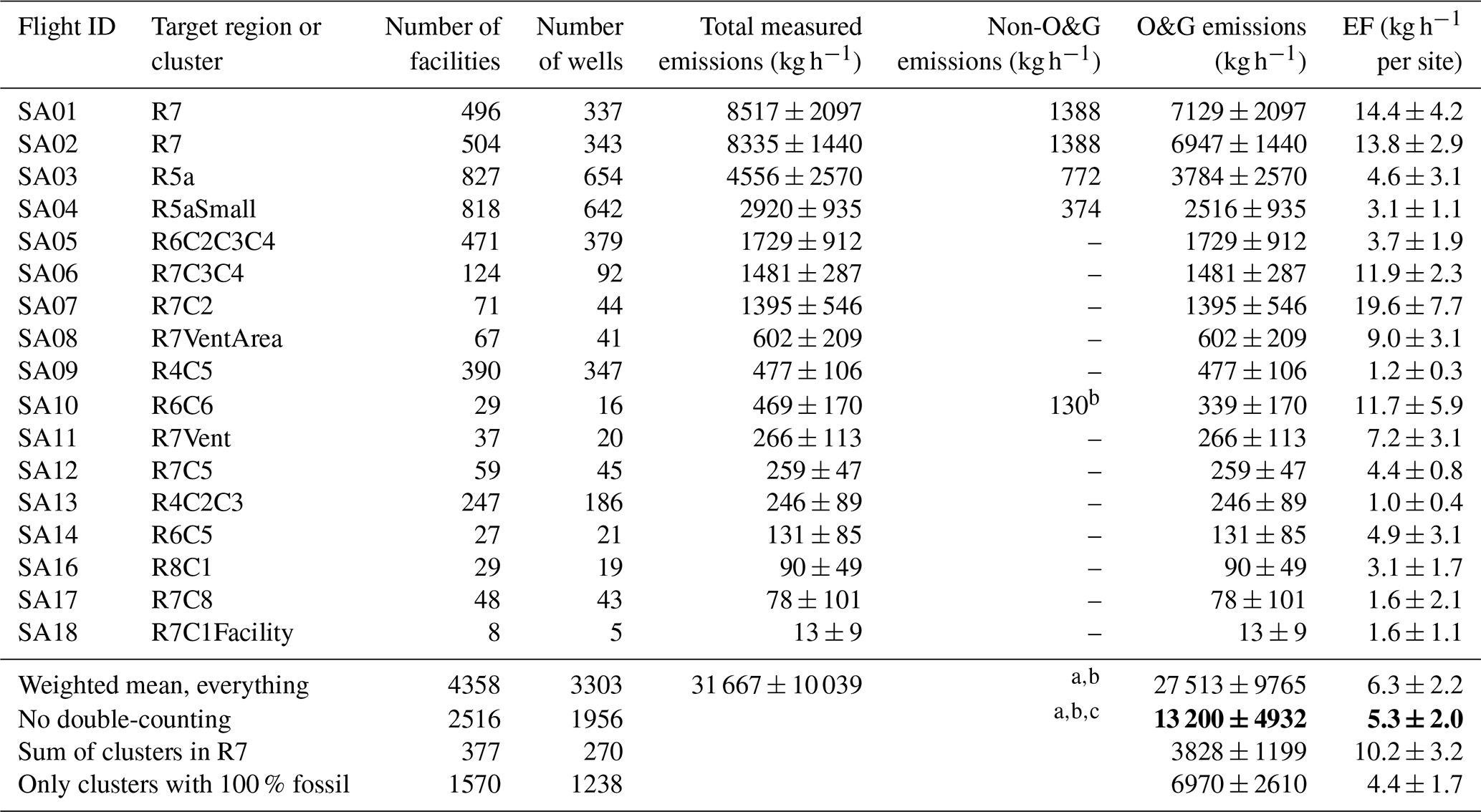
^a Considering the absolute non-O&G emissions from the TNO-CAMS inventory for the large regions and 100 % O&G contribution for the clusters. ^b Accounting for the landfill within R6C6. ^c Excluding cluster quantifications in R7.

Different inventories (E-PRTR, TNO-CAMS v6.0, and EDGAR v7.0) were consulted to obtain information about the non-O&G contributions; however, these inventories are generally not designed to distribute emissions across sectors on such small scales. TNO-CAMS and EDGAR have a coarse spatial resolution and do not include production clusters, so they are not suitable to assess the emissions distribution across sectors in such clusters. With the exception of R6C6, which includes a landfill listed in E-PRTR for the year 2019, for all other production clusters, E-PRTR does not indicate any major farms or landfills. The ground teams did not observe significant non-O&G sources in the smaller production clusters. Therefore, we ascribe 100 % of the total emissions in clusters to O&G production. For the large regions R7 and R5a, we use the estimated absolute non-O&G emissions from TNO-CAMS and subtract them from the measured emissions to correct for non-O&G-related emissions.

The emission factors (EFs) provided in Table 1 are calculated using the number of total active (e.g., producing or operating) infrastructure elements within the target regions because the measurements do not allow us to distinguish between different parts of the infrastructure. The emission factors vary widely among the individual clusters, from 1.0 to 20 kg h⁻¹ per site. This is partly due to the inhomogeneous distribution of the emissions, where a few sites are responsible for a large share of the emissions. A contributing factor is that each quantification yields an emission estimate for the specific moment in time of the measurement. The variability in our cluster-specific emission factors may partly represent the episodic tendency of O&G super-emitters. However, given the generally large number of infrastructure elements within the target regions, the reported numbers should still reflect representative averages for the clusters and regions and also over longer periods. Note that the timing of our measurements is random, and the total facility sample size (N = 4358, including duplicates; see below) is large. To address the challenge of emissions variability and inhomogeneity, we employ a weighted averaging approach based on facility numbers.

The sum of all emissions from the airborne CH₄ emission measurements (SA01–SA18) from all flights reaches 31 700 kg h⁻¹, accounting for 4358 active sites measured during all flights combined (Table 1). This results in an EF of 7.3 kg h⁻¹ per site after simple division. However, this EF is biased for two reasons: (i) not all emissions measured (31 700 kg h⁻¹) are from O&G sources and (ii) double- to triple-counting of emissions is present in the total sum; e.g., R5a and R7 were measured 2 or 3 times. The former point results in overestimation of EFs from O&G activities, and the latter point results in biasing the average EF towards emission rates of sources that were measured more than once. Therefore, we performed several analyses to address these two points.

In total, in addition to cluster-focused flights for R7, two regional flights each were performed for R7 and R5a, which results in triple-counting of emissions for R7 and double-counting of emissions for R5a in the total sum of 31 700 kg h⁻¹. Hence, we used average emission rates from the regional measurements targeting R7 and R5a individually (SA01 and SA02 for R7 and SA03 and SA04 for R5a). For the regions R4, R6, and R8, no regional flights were performed, and cluster-focused quantifications were performed. We used the sum of emissions from these clusters as the total emissions for these regions. These corrections result in cumulative emissions of 13 200 ± 4932 kg h⁻¹ for these regions, accounting for 2516 active sites, which results in an EF of 5.3 ± 2.0 kg h⁻¹ per site.

Acting on the field observations and inventory information, emissions from all clusters can be assigned to O&G activities, except for in R6C6. After deducting reported emissions for the landfill within the boundaries of R6C6 and adding the measured emissions from other clusters, we reach total emissions of 6970 ± 2610 kg h⁻¹ for 1570 sites, which results in an EF of 4.4 ± 1.7 kg h⁻¹ per site.

Both EFs, 5.3 ± 2.0 and 4.4 ± 1.7 kg h⁻¹ per site, overlap with the EF of 5.4 kg h⁻¹ (the 95 % CI is 3.6–8.4 kg h⁻¹) for oil production per site reported from ground-based measurements by Stavropoulou et al. (2023). However, both EFs from the airborne measurements fall on the lower side of the EF from the ground-based measurement. This could be explained as follows:

• i.

  It is assumed in Eq. (1) that all emissions within the flight boundaries are transported horizontally and captured during the flights. However, during the ROMEO campaign, the low-wind-speed conditions and high solar radiation could have resulted in vertical transport, which was not measured during the airborne measurements. It is possible that the area mass balance quantifications in the flat and arid region R5a in southern Romania may be biased slightly low due to partial loss of CH₄ out of the boundary layer during hot and convective conditions or due to the fact that stable transport conditions had not yet become established over the large regions.

• ii.

  The quantifications reported by Stavropoulou et al. (2023) were focused on oil production for which gas production, which is mostly methane, is not favorable and is hence released, which we were also able to observe through optical gas imaging cameras. This release produces favorable conditions at the production sites for the prevention of two-phase conditions in the pipelines and collection and processing systems.

These two reasons individually or combined could explain this average difference between the EFs derived from airborne and ground-based measurements. The difference between the two EFs derived from the airborne measurements, 5.3 ± 2.0 kg h⁻¹ per site from regional measurements and 4.4 ± 1.7 kg h⁻¹ per site from the clusters only, could be explained by the presence of large emitters outside the clusters but within the regional boundaries.

As the campaign airport was located close to the city of Ploiesti in region R7, the majority of cluster quantifications were carried out in R7 for logistical reasons, and many of the dense production clusters in R7 were quantified. This allows us to compare the sum of the emission rates determined from cluster quantifications to the emission factors from regional quantifications. The cluster flights in region R7 quantified a total of 377 O&G sites, which is 75 % of the 500 sites that were quantified in the regional flights. The quantified emissions from the cluster flights (3828 ± 1199 kg h⁻¹) amount to 54 % of the total emissions quantified in the regional flights after subtracting non-O&G emissions (about 7038 ± 1769 kg h⁻¹ from two independent flights; Table 1). This indicates a possible underestimate of non-O&G emissions in the inventories for R7, which includes the large city of Ploiesti. Alternatively, some super-emitters may exist outside the quantified clusters, which would increase the regional estimate. Nevertheless, the region and cluster flights show a reasonable level of consistency in region R7. The emission factors further support this alignment, with the weighted sum of the clusters being equal to 10.2 ± 3.2 kg h⁻¹ per site compared to about 14.1 ± 3.6 kg h⁻¹ per site for the regional flights. While the measurement-based quantifications for region R7 from the two flights are 7129 ± 2097 and 6947 ± 1440 kg h⁻¹, reported emissions for O&G activities in TNO-CAMS v6.0 and EDGAR v7.0 for this region were 3112 and 73 kg h⁻¹, respectively. This shows the large difference between inventories and particularly a large underestimation in EDGAR v7.0 by a factor of about 100. The underestimation of O&G emissions from production areas in the earlier versions of the EDGAR inventory has also been noted previously (Maasakkers et al., 2016; Scarpelli et al., 2020; Sheng et al., 2017). The causes of and discrepancies between of the difference observed between the measurements and the inventories require further investigation, which is beyond the scope of this study.

The aircraft-based quantifications indicate that per-site emission factors from region R7 are higher than from the other regions. At the same time, R7 was best covered in terms of mass balance determinations, so it is the most reliable estimate. From the site-level quantifications carried out on the ground, it was not apparent that per-site emission rates varied between different regions (Stavropoulou et al., 2023; Delre et al., 2022; Korbeń et al., 2022).

When we use the derived emission factor of 5.3 ± 2.0 kg h⁻¹ per site and scale this up to the entire production basin in southern Romania, with more than 4900 active sites, annual estimated emissions reached 227 ± 86 kt CH₄ yr⁻¹. If the derived EF also applies to the infrastructure in other parts of Romania, the inferred country-scale emission rate from about 7400 active sites in 2019 is 344 ± 130 kt CH₄ yr⁻¹. Reported emissions to the UNFCCC for Romania in category 1.B (fugitives) include 53 kt CH₄ yr⁻¹ for activity 1.B.2.b (natural gas), 38.2 kt CH₄ yr⁻¹ for activity 1.B.2.c (venting and flaring (oil, gas, combined oil and gas)) and 10.4 kt yr⁻¹ for activity 1.B.2.a (oil) (UNFCCC, 2023b). This adds up to 101.6 kt CH₄ yr⁻¹, about 3 times less than our estimate. Our estimate does not include emissions from infrastructure operated by other operators, for example the large gas production region in the Transylvanian Basin.

For comparison, we repeated the analysis using the EDGAR v7.0 inventory to estimate non-O&G sources for the large regions (see Supplement, Table S6). After removing double-counting and adjusting for emissions from other sources as described previously, the total emissions attributed to O&G production that were measured are 12 732 ± 4932 kg h⁻¹. This is slightly lower than the total emissions estimated using the TNO-CAMS v6.0 inventory, 13 200 ± 4932 kg h⁻¹, indicating a larger fraction of non-O&G sources in the EDGAR v7.0 inventory. The inferred O&G emissions, taking into account the non-O&G emissions from the EDGAR inventory, result in a facility-weighted emission factor of 5.1 ± 2.0 kg h⁻¹ per site, consistent with the 5.3 ± 2.0 kg h⁻¹ per site when using TNO-CAMS v6.0 for the non-O&G sectors. It is important to note that the inventory estimates for the non-O&G sectors do not differ strongly between EDGAR v7.0 and TNO-CAMS v6.0 in the regions where we apply the corrections. However, this is not the case for all regions in the southern Romanian production basin. Table S7 in the Supplement shows that the discrepancies between the two inventories can become large. Specifically, in EDGAR v7.0, the non-O&G emissions are higher than those in TNO-CAMS v6.0, nearly double in some cases. Moreover, O&G emissions are very low in EDGAR, whereas they contribute to almost half of the emissions in TNO-CAMS v6.0. Because of this more balanced contribution from all sources, we use the estimates from TNO-CAMS v6.0 for our central emission factor estimate and for the upscaling.

3.2 Qualitative information from measurement–simulation comparisons

3.2.1 Example comparison of meteorology and CH₄ for a mass balance flight

Figure 3 shows an example of a comparison between measurements along the SA mass balance flight from 17 October 2019 and results from the COSMO-GHG and MECO(3) models. The top two panels show simulated and measured CH₄ mole fractions along the flight track, and the bottom two panels show the vertical CH₄ profiles in the simulations along the flight track above the changing orography (black). During this flight, four different clusters and combinations of clusters were circled multiple times at different altitudes; the flight altitude is included in the bottom panels as dashed black lines. The repeating orographic patterns guide the eye in following the circular flight patterns around the clusters and are numbered in white. The colored contours illustrate the vertical CH₄ profiles along the flight track. The measured plume in the first, largest cluster is captured relatively well by the simulation for some of the cycles, but during some cycles the flight track is partly above the boundary layer in the models, and the peak is not fully captured. During cycles four and five, the observations suggest that the aircraft was flying above the boundary layer in reality also, but one sharp, narrow peak was still observed after the highest orographic peak in the measurements, which is missing in the simulation. For the second cluster, which was cycled 12 times, the COSMO-GHG model captures the plumes better than the MECO(3) model. For both models, the simulated and measured CH₄ mole fractions show a consistent transition out of the boundary layer in cycles seven to nine, indicating good representation of the boundary layer height in the models. For the third cluster, the models are missing the large, sharp peaks, indicating missing emissions in this cluster. In addition, the MECO(3) model simulates higher plumes when the flight track was in the model boundary layer but lower plumes when the flight track was outside the boundary layer. For the last cluster, the simulated and measured elevations are small and relatively consistent for COSMO-GHG, but the MECO(3) model simulates some larger plumes spanning more than one cycle, indicating larger-scale upwind contamination, which was also documented in the observations.

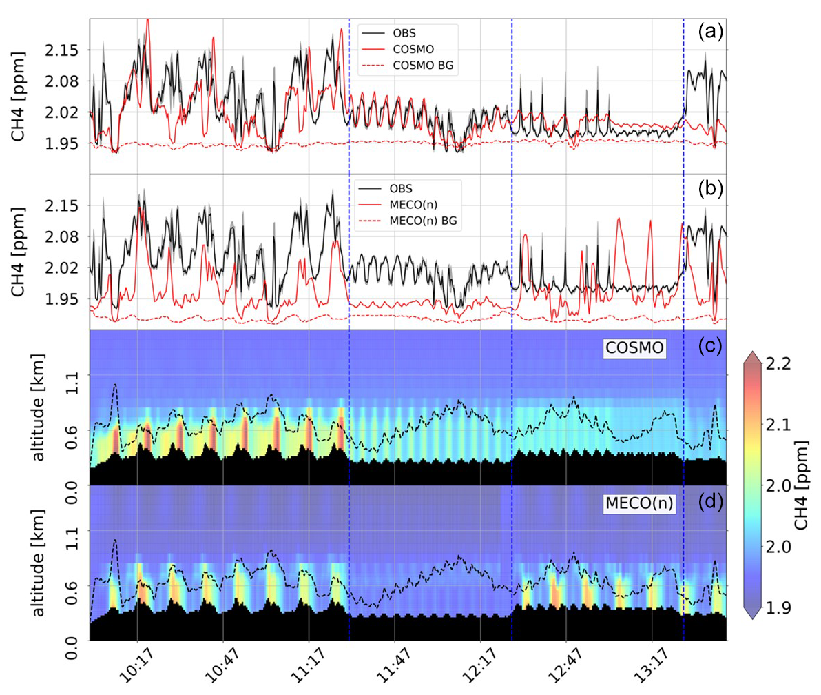
Figure 3 Measurements and simulation results of (a, b) CH₄ mole fractions along the flight track and (c, d) the vertical CH₄ profile along the flight track as simulated by the COSMO model (a, c) and the MECO(3) model (b, d). Model background fields are shown as dashed lines in panels (a) and (b). Panels (c) and (d) also include the flight tracks as dashed black lines, and the black contours at the bottom show the orography in this mountainous terrain; the repeating patterns illustrate individual cycles around the clusters R6C2C3C4, R6C5, R6C6, and R6C7, and cycles are numbered in white. The flight around cluster R6C7 did not allow successful emission quantification because of an upwind influence and is therefore not included in Table 1.

A similar analysis was performed for each flight, with the goal to identify plumes where either the simulation results or the measurements indicated that the respective circle was flown outside the simulated or actual boundary layer. In this case, the respective plume was not retained for the measurement–simulation comparison. In total, 10 out of 200 individual plumes were rejected this way. In addition, 66 circles around clusters that were influenced by signals from upwind sources were excluded.

3.2.2 Model performance in terms of meteorology

As mentioned above, the low winds during the campaign period presented difficult meteorological conditions for emissions quantification. We performed a thorough meteorological analysis to identify days when the meteorological conditions agree well between the two models and the measurements. The results are shown in Sect. S1, which illustrate that it was not possible to identify days when the meteorological conditions agree well between the two models and the measurements. Therefore, it was decided not to focus on individual days or flights. Rather, in the following, we compare the measured and simulated plume areas statistically across all available flights. This is done to investigate whether correlation between measured and simulated CH₄ enhancements from the raster flights, which cover a wider region, is similar to the one between the individual plumes quantified during the mass balance flights. The analysis, which is described in the section below, can also possibly identify regional differences and can be used to derive approximate scaling factors for the raster flights in comparison with the mass balance flights.

3.3 Measurement–model comparison of plume areas for mass balance flights

We first evaluate plume-level data from the individual mass balance flights because for these flights we have measured emission rates from the mass balance approach. Thus, we can compare the measured and simulated plume areas and derive a correction factor for the emission rates assumed in the model that would bring the measured and simulated plumes into agreement. A total of 256 plumes were identified, 66 of which were rejected, and 190 plumes were retained for analysis. Figure 4 shows the plume area comparison of these 190 plumes from the SA mass balance flights and COSMO-GHG and MECO(3) models.

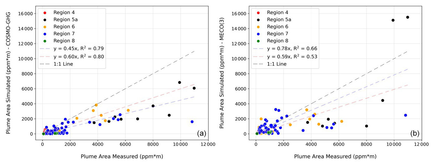
Figure 4 Comparisons between plume areas calculated from measurements and simulations with COSMO-GHG (a) and MECO(3) (b). Dashed blue lines show linear fits to all data and dashed red lines linear fits to the plumes from the clusters only, without the points from the larger regions. Plots zooming in on the region of plume areas up to 2000 ppm m are shown Fig. S1.

For mass balance flights around production clusters, each circle around a cluster results in one or a few downwind plumes (which are integrated into our analysis), but for mass balance flights targeting larger regions, numerous well-separated plumes can generally be quantified from a single circle. The high scatter in the comparison between simulated and measured plume areas can be ascribed to a number of factors, for example: (i) large variability in actual emissions from different source areas (here – production clusters), including the important role of super-emitters; (ii) difficult meteorological conditions with low wind leading to variable plume representations in both the real atmosphere and the model; (iii) over- or underestimates associated with the dynamics of the planetary boundary layer; and (iv) variable measurement distance from the emission points. The scatter in the comparison of plume areas with MECO(3) results is even larger than for the COSMO-GHG model. This is ascribed to the fact that the meteorological fields in COSMO-GHG are nudged to observations, whereas MECO(3) nudges only the global model instance, implying more degrees of freedom within the nested instances to develop their own (sub-synoptic) meteorological situation, which might deviate from the data used for nudging. Indeed, the meteorological evaluation (see Sect. S1) shows that the meteorological fields in COSMO-GHG (directly nudged) are closer to the observed meteorological parameters than to MECO(3), as expected.

Nevertheless, despite the variability, it is evident that most of the points fall well below the 1 : 1 line, which means that the simulated plume areas along the flight track that were generated with an assumed emission factor of 1 g s⁻¹ per site, thus 3.6 kg h⁻¹ per site, generally underestimate the measured plume areas. The further the points fall below the 1 : 1 line, the higher the implied mismatch in the emission rate that was assumed in the model. A linear fit to all the measured and simulated plumes has a slope of 0.44 for COSMO-GHG and 0.78 for MECO(3). When we exclude the points from the larger regions, where the measured plumes are often further away from the source regions, the slopes change slightly to 0.56 for COSMO-GHG and to 0.62 for MECO(3). This suggests that the assumed emission rate in the model is on average underestimated by about a factor of 2. However, quantitative interpretation is problematic in this approach, since the slope of the linear fit is largely determined by a relatively small number of plumes with large plume areas. Furthermore, the sampling is biased towards clusters where more circles were flown (i.e., circles at more altitude levels) and does not consider the number of facilities per cluster. In addition, there may be systematic biases in the models, e.g., due to model resolution or meteorological conditions (as discussed above), that lead to smaller plume areas in the models compared to the measurements. For the present purpose, we will compare the slope of observed and simulated plume areas from the mass balance flights determined here with the slope of observed and simulated CH₄ enhancements from the raster flights in Sect. 3.4 to investigate whether the enhancements observed during the raster flights qualitatively agree with the ones from the mass balance flights.

3.4 Measurement–model comparison of plume areas for raster flights

Figure 5 shows the comparison of the integrated enhancement above the background along the flight tracks for the CH₄ mole fractions measured during the raster flights and simulated with the two models. The scatter for these integrated enhancements is smaller than for the individual plume areas shown in Fig. 4., which likely reflects the fact that the integrated enhancements are the sum of numerous plumes, and high and low values average out for the integrated enhancements.

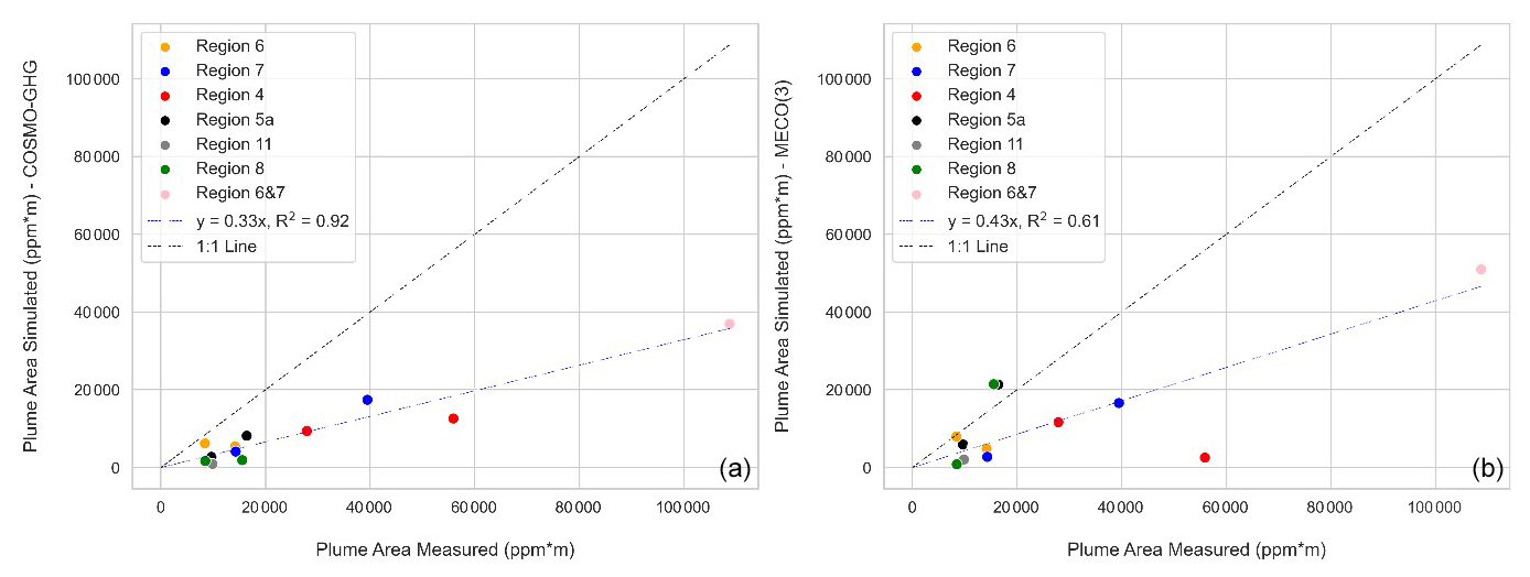
Figure 5 Comparison between integrated CH₄ enhancements from measurements during raster flights on the BN2 aircraft and simulations along the flight tracks with COSMOS-GHG (a) and MECO(3) (b). Different colors represent different regions. Linear fits to the data are shown as dashed blue lines, and the 1 : 1 line is shown as the dashed black line.

Similar to the plume area comparison from the mass balance flights (Fig. 4), most of the points fall below the 1 : 1 line, again indicating that the emission rate of 3.6 kg h⁻¹ per site assumed in the models is insufficient to explain the observed concentrations. The slopes of the orthogonal linear regressions of 0.43 and 0.33 for the two different models are even lower than for the mass balance flights above, indicating a possible underestimate by up to a factor of 3 in the assumed emission rate. Still, the slopes are in a similar range as the slopes from the mass balance flights in Fig. 4. It is important to note that these slopes were derived from the simulated fields under similar conditions as the ones for the individual plumes from the clusters. Thus, whereas various factors could cause systematic under- or overestimates in simulated versus measured CH₄ enhancements, the similar slopes obtained for the two types of flights suggest that the emission characteristics of the plumes observed during the mass balance and raster flights are compatible. Thus, the emission factors derived for a limited number of clusters in Sect. 3.3 are likely representative of the larger areas covered in the mass balance flights and thus for a large fraction of the southern Romanian O&G production infrastructure. We conclude that the CH₄ enhancements observed by the BN2 aircraft during the raster flights generally support the emission factors derived in Sect. 3.1 from the mass balance approach.

4 Conclusions

Airborne measurements of methane performed from two aircraft during the ROMEO 2019 campaign were evaluated to obtain emission rate estimates representative of production clusters and larger regions in the O&G production basin in southern Romania. Emissions determined from a mass balance approach yield a wide range of instantaneous emission factor estimates between different clusters, supporting the heterogeneity of emissions across individual sites, regions, and time. Assessment of the O&G emissions from flights around larger regions is difficult because of the unknown contribution of emissions from other sectors. From mass balance estimates covering a total of 2516 sites, when using the TNO-CAMS inventory to derive emissions from non-O&G sources for the large regions, and with the assumption of 100 % of the observed emissions in the smaller clusters originating from O&G production, we derive total emissions of 13 200 ± 4932 kg h⁻¹ for the regions covered in southern Romania. This results in a facility-weighted emission factor of 5.3 ± 2.0 kg h⁻¹ per site, consistent with the previously published estimate from ground-based quantifications of 5.4 kg h⁻¹ from oil production per site (range of 3.6–8.4 kg h⁻¹ per site; Stavropoulou et al., 2023). The facility-weighted average for 1570 facilities in dense production clusters, where we are certain that the dominant contribution is from the O&G infrastructure, is 4.4 ± 1.7 kg h⁻¹ per site, aligning with the estimate from larger regions. Using an EF of 5.3 kg h⁻¹ per site to scale up to the national scale results in an annual emission rate estimate of 344 ± 130 kt CH₄ yr⁻¹, which is about 3 times higher than the UNFCCC-reported national emissions from the O&G industry for Romania. Mole fraction measurements carried out in raster flight tracks over wider areas lacked meteorological measurements and therefore could not be used to derive direct estimates of emission rates. To support the evaluation, simulations with two numerical atmospheric models were carried out, and the simulated CH₄ fields were compared with the measurements. Due to the difficult meteorological conditions, direct quantitative evaluation remains challenging, but the comparison of observed and simulated enhancements consistently suggests that the prior emission rate of 3.6 kg h⁻¹ per site used in the models is too low. In addition, the correlation of measured and simulated CH₄ enhancements for the raster flights over larger areas is consistent with the correlations observed in mass balance flights around well-defined production clusters, indicating the validity of the derived emission factors for a large part of the southern Romanian O&G production region. Airborne measurements for the regions and clusters where ground-based surveys can also be applied can provide important additional insights, such as (i) the influence of super-emitters is included as a realistic fraction in the total airborne measured emissions, while super-emitters may be either missed or accidentally overrepresented in ground surveys; (ii) the influence of non-O&G sources on total emissions can be studied; and (iii) airborne quantification can cover large areas in a much shorter time compared to ground-based quantification. We conclude that the top-down emission estimates derived here from airborne surveys over larger regions support the previously published emission rate estimates derived from ground-based bottom-up quantifications during the ROMEO 2019 campaign. These results confirm that O&G methane emissions in 2019 were much higher within our study domain than were reported to UNFCCC and estimated in EDGAR.​​​​​​​