Understanding boreal summer UTLS water vapor variations in monsoon regions: a Lagrangian perspective

Water vapor in the upper troposphere and lower stratosphere plays a crucial role for climate, affecting radiation, chemistry, and atmospheric dynamics. This study applies a simplified Lagrangian method to reconstruct stratospheric water vapor based on satellite observations from the Stratospheric Aerosol and Gas Experiment III on the International Space Station (SAGE III/ISS) and the Aura Microwave Limb Sounder (MLS). The objective is to improve understanding of moisture enhancements in the Asian and North American monsoons and to identify the key factors contributing to reconstruction biases. The performance of Lagrangian reconstructions significantly improves with the size of trajectory ensembles but exhibits a general dry bias. The reconstruction represents the summertime local water vapor maximum well in the Asian monsoon, particularly above the tropopause, but not in the North American monsoon. The main dehydration region diagnosed from trajectories indicates that water vapor in the Asian monsoon is predominantly controlled by local tropopause temperatures. The dry bias in reconstructions below the tropopause over the Asian monsoon shows a positive correlation with convection intensity, particularly in the western part of the monsoon region, suggesting that underestimated moistening from convection may contribute to this bias. Water vapor mixing ratios in the North American monsoon are largely influenced by long-range transport from dehydrated regions over southern Asia and additional local moistening. The limited performance of reconstructions in the North American monsoon is therefore likely linked to underestimation of local convection or uncertainties in long-range transport.

1 Introduction

Stratospheric water vapor (H₂O) is a potent greenhouse gas that can significantly amplify global warming due to its strong radiative effects and long residence time (Solomon et al., 2010; Riese et al., 2012). The amount of water vapor entering the stratosphere is largely determined by the freeze-drying of moist tropospheric air while ascending through the cold tropical tropopause (Brewer, 1949; Randel and Park, 2019; Smith et al., 2021). This process occurs mainly in the tropical tropopause layer (Fueglistaler et al., 2009), where air masses undergo slow diabatic ascent into the stratosphere over timescales of weeks to months. During ascend, the air masses travel thousands of kilometers in the horizontal direction and often sample the coldest tropopause regions (Holton and Gettelman, 2001). On the other hand, water vapor and ice can be directly injected into the Upper Troposphere and Lower Stratosphere (UTLS) by deep, overshooting convection and related strong vertical updrafts near the convective centers on timescales of minutes (Jorgensen and Lemone, 1989; Schwartz et al., 2013). Such convection-driven transport has been reported to occur frequently in the tropics and over North America during boreal summer (Homeyer et al., 2023). However, the extent to which this process affects stratospheric water vapor remains under debate (Randel et al., 2012; Avery et al., 2017; Ueyama et al., 2020; Jensen et al., 2020; Ueyama et al., 2023; Homeyer et al., 2023; Konopka et al., 2023).

During boreal summer, the UTLS over the Asian Summer Monsoon (ASM) and North American Monsoon (NAM) regions exhibits enhanced water vapor mixing ratios (Ploeger et al., 2013; Park et al., 2021; Clemens et al., 2022). This water vapor enhancement is strongly associated with seasonal variations in tropical tropopause temperatures and circulation (James et al., 2008; Uma et al., 2014) and is also attributed to intense convection that can transport water vapor directly into the UTLS (Fu et al., 2006; Yu et al., 2020). However, a detailed understanding of the mechanisms and interactions among regional convection, large-scale transport, and thermodynamic conditions in the monsoons and their effects on stratospheric water vapor has not been achieved, but is crucial for assessing related climate impacts.

The advection-condensation paradigm (Pierrehumbert and Roca, 1998; Liu et al., 2010) describes atmospheric water vapor distributions as being primarily controlled by advection through the saturation mixing ratio field. Lagrangian methods simulate the motion of air masses and quantify the dehydration process by identifying the coldest temperatures encountered along troposphere-to-stratosphere trajectories (TST). These coldest points, termed Lagrangian cold points (LCPs) (Fueglistaler et al., 2005), provide the essential diagnostic for applying the advection-condensation paradigm to stratospheric dehydration. Such methods have been widely applied to reproduce regional and temporal water vapor anomalies in the UTLS (Mote et al., 1995; Fueglistaler and Haynes, 2005; Liu et al., 2010; Schoeberl and Dessler, 2011; Smith et al., 2021).

Here, we aim at evaluating dehydration processes in the UTLS over the ASM and NAM regions from a Lagrangian perspective. The main research questions explored in this paper are:

• How well can UTLS water vapor mixing ratios in the ASM and NAM be reconstructed using a simplified Lagrangian modelling method, especially in comparison to the tropics (here defined as 35° S–35° N)?

• Are the moisture enhancements observed within the ASM and NAM anticyclones locally or remotely controlled and which regions contribute most strongly to these enhancements?

• Are differences between the reconstruction and the observation related to particular processes (e.g., convection)?

We primarily use satellite observations from the Stratospheric Aerosol and Gas Experiment III on the International Space Station (SAGE III/ISS) which have relatively high vertical resolution compared to other satellite observations. In addition, we use observations from the Aura Microwave Limb Sounder (MLS), which provide daily global coverage and have been widely used in studies of stratospheric water vapor (Mote et al., 1995; Liu et al., 2010; Nützel et al., 2019). To reconstruct the satellite observations, we perform Lagrangian backward trajectory simulations with the trajectory module of the Chemical Lagrangian Model of the Stratosphere (CLaMS), driven by the fifth generation European Centre for Medium-Range Weather Forecasts atmospheric reanalysis (ERA5). The reconstruction performance in capturing UTLS water vapor distributions is evaluated by comparison with the satellite observations and by contrasting the monsoon regions with the tropics, where similar methods have been successfully applied in the past (Fueglistaler et al., 2005; Hasebe and Noguchi, 2016; Smith et al., 2021). Finally, we determine the dehydration regions and investigate factors contributing to differences between reconstructions and observations, with particular focus on the role of deep convection.

This paper is organized as follows: Sect. 2 describes the datasets, model, and reconstruction method. Section 3 presents the main results, including the evaluation of Lagrangian water vapor reconstructions and analysis of dehydration regions. Section 4 examines possible causes of reconstruction biases and their links to convection. Section 5 summarizes the conclusions.

2 Data and Methods

2.1 Satellite observations

2.1.1 MLS

The Microwave Limb Sounder (MLS) instrument on the Aura satellite (Waters et al., 2006) has provided global profiles of water vapor, ozone, carbon monoxide, and other trace gases since August 2004 (https://www.earthdata.nasa.gov/learn/find-data/near-real-time/mls, last access: 1 September 2023). MLS offers comparatively high sampling with about 3500 profiles per day. In this study, we use version 5.0 (v5.0) data, which provide water vapor profiles with 2.1–3.5 km vertical resolution (Lambert et al., 2017), and about 3.0 km resolution in the lower stratosphere (Read et al., 2007). We focus on water vapor measurements for August 2017–2019 in the tropics (35° S–35° N). For visualization in Fig. 1, MLS water vapor profiles are gridded into 10° × 20° (latitude × longitude) bins. Further details on MLS water vapor and retrieval methods are given in Livesey et al. (2020).

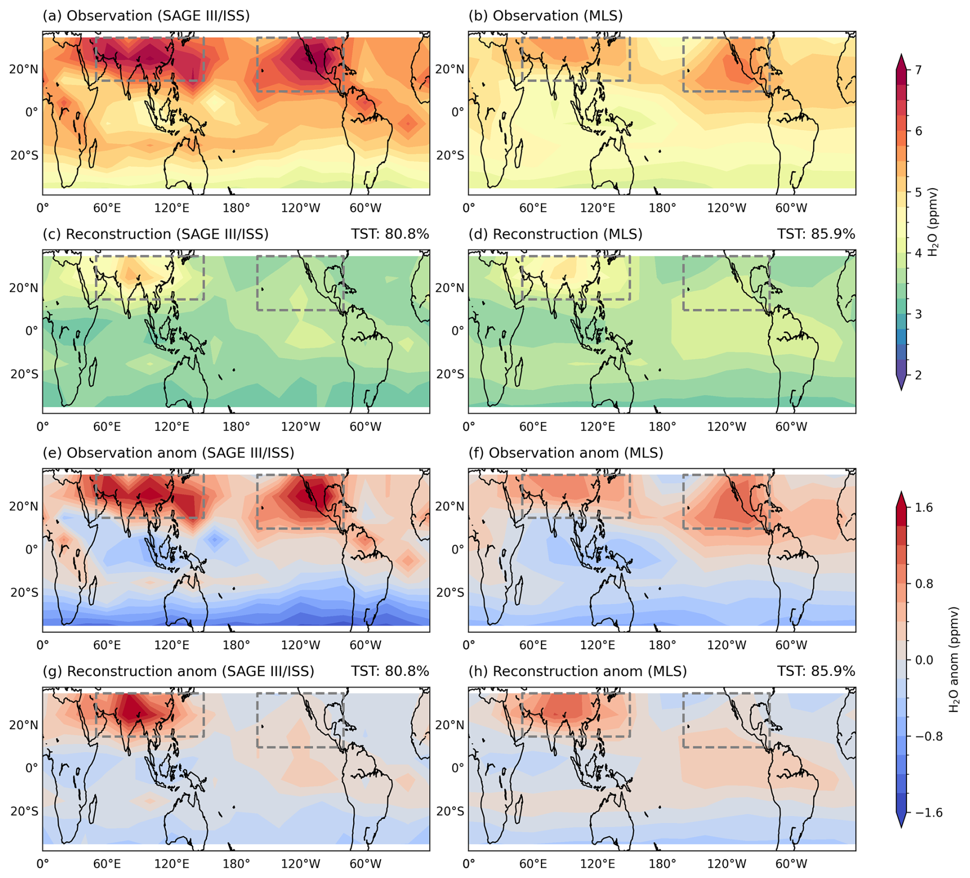
Figure 1 Horizontal distributions of water vapor (H₂O) mixing ratios and anomalies in August. Panels (a)–(b) show observed water vapor mixing ratios, (c)–(d) reconstructed mixing ratios from experiment LAG, and (e)–(h) the corresponding spatial anomalies, based on SAGE III/ISS (2017–2022) at 16.5 km (left) and MLS (2017–2019) at ∼ 16.3 km (right). The anomalies are calculated relative to the tropical mean (35° S–35° N). Grey boxes indicate the ASM region (15–35° N, 50–150° E) and NAM region (10–35° N, 160–80° W). Reconstructions include both TST and non-TST trajectories; the fraction of TSTs is given in the upper right of (c)–(d) and (g)–(h).

2.1.2 SAGE III/ISS

The Stratospheric Aerosol and Gas Experiment III on the International Space Station (SAGE III/ISS), launched on 19 February 2017 (Cisewski et al., 2014), provides measurements of aerosol, water vapor, and ozone between 70° S and 70° N using solar occultation, lunar occultation, and limb scattering. In this study, we use the Level 2 (L2) Solar Event Species Profiles (HDF5) Version 5.3 (v5.3) data product (https://asdc.larc.nasa.gov/project/SAGE III-ISS/g3bssp_53, last access: 11 September 2023). According to Davis et al. (2021), SAGE III/ISS v5.1 water vapor measurements agree well with MLS v5.0 in the stratosphere, with SAGE III/ISS reporting values about 0.5 ppmv (10 %) lower in the 15–35 km altitude range. However, SAGE III/ISS v5.1 profiles were affected by low-quality data from aerosol and cloud interference (Park et al., 2021; Davis et al., 2021). These issues – such as failed retrievals and increased sensitivity to elevated aerosol loading – were largely mitigated in Version 5.2 and later, as documented in the SAGE III/ISS Data Products User's Guide (https://asdc.larc.nasa.gov/documents/sageiii-iss/guide/DPUG_G3B_v05.30.pdf, last access: 11 September 2023).

We focus on water vapor measurements for August 2017–2022 in the tropics (35° S–35° N). Note that the periods considered here for the two satellite datasets are different. For MLS, we use the period 2017–2019, whereas for SAGE III/ISS we extend the period to 2017–2022 to ensure sufficient spatial coverage over the considered region. The shorter MLS period is chosen because the large volume of MLS data provides reliable statistics already for this three-year period but makes the trajectory calculations computationally challenging, particularly when large trajectory ensembles are launched for each measurement point (specific numbers of trajectories are now provided in Sect. 2.3.1). For SAGE III/ISS, extending the period to 2017–2022 improves the sampling coverage without introducing no significant differences relative to 2017–2019 (cf. horizontal water vapor distributions in Figs. 1 and S1 in the Supplement), thereby justifying the use of the longer period in the analysis.

The SAGE III/ISS v5.3 water vapor profiles are retrieved on a 1.0 km grid and interpolated to 0.5 km from 0.5–60.0 km altitude. Following Davis et al. (2021), we apply a 1-2-1 vertical smoothing on the 0.5 km grid, yielding a final vertical resolution of 2 km. For the horizontal distributions shown in Fig. 1, the data are binned at 10° × 20° (latitude × longitude) resolution, requiring at least five profiles per bin, following the approach of Park et al. (2021) for SAGE III/ISS v5.1.

2.2 OLR

We use daily mean outgoing longwave radiation (OLR) as a proxy for deep convection. The OLR data are obtained from the National Oceanic and Atmospheric Administration (NOAA) Climate Prediction Center (CPC) (https://psl.noaa.gov/data/gridded/data.cpc_blended_olr-2.5deg.html, last access: 22 May 2024). The CPC blended OLR Version 1 dataset combines Level 2 OLR retrievals from NASA's Cloud and Earth Radiant Energy System, NOAA/NESDIS Hyperspectral measurements, and High-resolution Infrared Radiation Sounder data. The gridded daily OLR covers the period from 1991 to the present on a 2.5° × 2.5° (latitude × longitude) global grid and also provides temporal anomalies, defined as deviations from the monthly mean at each grid point. To derive OLR indices for the ASM, we average the temporal anomalies within two horizontal boxes following Randel et al. (2015): (i) an OLR-West box covering 20–30° N, 50–80° E, and (ii) an OLR-East box, covering 20–30° N, 80–110° E. Note that, while OLR is a commonly used proxy for convective intensity, it has limitations in identifying deep convection due to its reliance on infrared measurements. These measurements can underestimate cloud-top temperatures, particularly over land and for aged anvil clouds (Liu et al., 2007).

2.3 Models

2.3.1 CLaMS trajectory module

The Chemical Lagrangian Model of the Stratosphere (CLaMS) is an offline Chemistry Transport Model (CTM) for simulating transport and chemical processes in the atmosphere (McKenna et al., 2002; Konopka et al., 2022). CLaMS employs a Lagrangian framework in which individual air parcels are tracked, enabling detailed representation of atmospheric dynamics and chemistry particularly in regions of strong gradients. In this study, we use the trajectory module of CLaMS 2.0 for the calculation of air parcel trajectories (https://clams.icg.kfa-juelich.de/CLaMS/traj, last access: 20 September 2023). The driving meteorological fields are from ERA5, with 1° × 1° horizontal resolution, 137 vertical hybrid layers, and 6 h temporal resolution (Hersbach et al., 2020). We perform 180 d backward trajectory calculations, launching each air parcel from the exact spatial location and time of the satellite observations within the tropics (30° S–30° N). For August 2017–2022, SAGE III/ISS provides 149, 203, and 2292 profiles for the ASM, NAM, and tropics, respectively. For August 2017–2019, MLS provides 7801, 10 223, and 126 981 profiles for the ASM, NAM, and tropics, respectively. Taking the ASM and SAGE III/ISS observations as an example, the number of calculated trajectories is given by 149×10 (profiles × altitude levels) for the simulation experiment with one trajectory launched at each measurement point (termed LAG_single, see Sect. 2.3.2 for definitions of the experiments). Likewise, the number of trajectories is $\mathrm{149}\times \mathrm{10}\times \mathrm{51}$ (profiles × altitude levels × trajectory ensemble size) for the experiment with trajectory ensembles started at each measurement (LAG). Accordingly, the total number of trajectories for the single trajectory experiment LAG_single is 1490 for the ASM, 2030 for the NAM, and 22 920 for the tropics, while for the trajectory ensemble experiment (LAG) these values increase to 75 990, 103 530, and 1 168 920, respectively. For MLS, the corresponding numbers of trajectories are 39 005 for the ASM, 51 115 for the NAM, and 634 905 for the tropics in the LAG_single experiment. In the LAG experiment, these values are multiplied by 51, yielding 1 989 255 for the ASM, 2 606 865 for the NAM, and 32 379 155 for the tropics, respectively.

2.3.2 Water vapor reconstruction

We reconstruct water vapor mixing ratios from saturation at the coldest temperature and the corresponding air pressure along the trajectories. The reconstructed stratospheric water vapor mixing ratios are calculated as:

$${{\mathrm{H}}_{\mathrm{2}}\mathrm{O}}_{\text{ppmv}}=\mathrm{1.0}\times {\mathrm{10}}^{\mathrm{6}}\cdot {\displaystyle \frac{e_{\text{sat}}}{P-e_{\text{sat}}}},e_{\text{sat}}={\displaystyle \frac{{\mathrm{10}}^{\left(\frac{A}{T}+B\right)}}{\mathrm{100}}},$$

where $A=-\mathrm{2663.5}$, B=12.537, T is the coldest temperature (K), and P the corresponding pressure (hPa) (Sonntag, 1994).

We present results from three types of reconstructions, termed LOC, LAG_single, and LAG, with the following characteristics:

• In LOC, T is defined as the minimum temperature in the ERA5 vertical temperature profile at the location of each SAGE III/ISS water vapor profile.

• In LAG_single, backward trajectories are initialized at each observation point in the UTLS, using its observed altitude, longitude, and latitude. T is the LCP temperature, i.e., the minimum temperature along each trajectory, and is then used to compute the water vapor reconstruction at that observation point as described above. For SAGE III/ISS, initialization altitudes range from 14.0 to 21.0 km at 0.5 km intervals. For MLS, pressure levels are converted to geopotential heights, and the levels closest to the SAGE III/ISS altitudes are used.

• In LAG, reconstructions are based on larger trajectory ensembles. For each observation point, 50 additional launch points are placed vertically at 10 m intervals above and below the altitude of the observation, resulting in 51 trajectories in total. For example, at 16.0 km (SAGE III/ISS), the ensemble covers 15.75–16.25 km in 0.01 km steps. The final reconstruction for each observation point is obtained by averaging the ${{\mathrm{H}}_{\mathrm{2}}\mathrm{O}}_{\text{ppmv}}$ values computed from the LCP temperatures along all 51 backward trajectories, thereby enhancing the vertical sampling around the observation altitude.

In LAG, the refinement of sampling is applied in the vertical direction, as vertical wind shear generally induces a stronger redistribution of air parcels than horizontal shear. As air parcels move, they are rapidly stretched into thin and horizontally extended layers due to quasi-horizontal, isentropic flow. This horizontal spreading gradually dilutes the parcels and lessens the necessity for denser horizontal sampling. For further details, please refer to Haynes and Anglade (1997), which explains how differential advection in the atmosphere drives vertical mixing and stretching of air parcels.

All backward trajectories are classified into two groups: those that ascend through the tropopause into the stratosphere, referred to as Troposphere-to-Stratosphere Transport (TST), and those that do not, referred to as non-TST. TST trajectories are defined as trajectories with launch points (observation points) above 370 K potential temperature that can be traced back to below 340 K potential temperature. For TST trajectories, reconstructed water vapor mixing ratios are calculated using the LCP temperatures. For non-TST trajectories, the reconstructed values are defined as the smaller of two quantities: the saturation mixing ratio based on LCP temperatures, and the climatological water vapor mixing ratio from MLS at the simulated origins of the backward trajectories, following the procedure of Fueglistaler et al. (2005).

3 Results

3.1 Performance of Lagrangian water vapor reconstruction

3.1.1 Spatial distributions

Figure 1a and b present the horizontal distributions of satellite observations in August at ∼ 16.5 km (around 100 hPa or 380 K), observed by SAGE III/ISS and MLS, respectively. The distributions from both satellite datasets show consistent spatial patterns, with the moisture maxima located over the ASM (15–35° N, 50–150° E) and NAM (10–35° N, 160–80° W). Figure 1c and d present corresponding water vapor reconstructions (experiment LAG). The reconstructions show dry biases across the tropics relative to observations. Except for the maxima over the NAM, the spatial patterns from both satellite datasets are broadly reproduced, particularly over the ASM. The anomaly fields (Fig. 1e–h) highlight these features more clearly. Over the ASM, the reconstructions capture the magnitude of the observed enhancement (1–2 ppmv) but with a more limited spatial extent, whereas over the NAM, the reconstructions only weakly reproduce the observed moisture enhancement by less than 1 ppmv. Compared with MLS, SAGE III/ISS observations show higher water vapor mixing ratios by ∼ 1 ppmv across most tropical regions (Fig. 1a, b), as well as larger moisture enhancements of ∼ 1 ppmv above the ASM and NAM in the anomaly feilds (Fig. 1e, f).

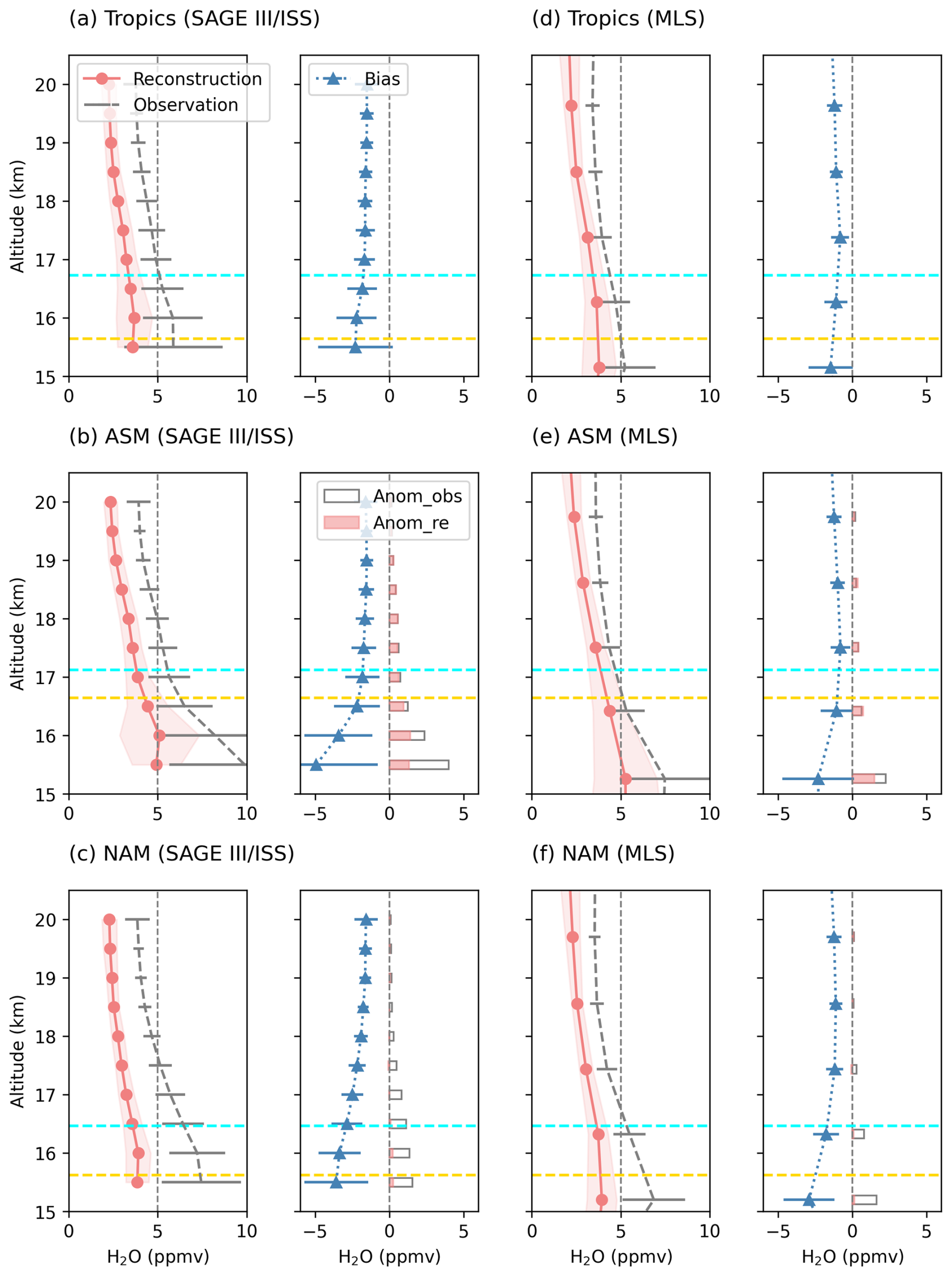
Figure 2 Vertical profiles of water vapor (H₂O) mixing ratios in August. Grey dotted lines show observations, coral lines show reconstructed values from experiment LAG (TST-only), and blue lines show reconstruction biases (reconstructed minus observed). Shading (or horizontal bars) indicates ±1 standard deviation around the respective profiles. Panels are averaged over the tropics (35° S–35° N; a, d), ASM (b, e), and NAM (c, f), with results based on SAGE III/ISS (left) and MLS (right). Cyan dashed lines mark the climatological cold point tropopause and yellow dashed lines mark the lapse rate tropopause (both from ERA5). In ASM and NAM panels (b, e; c, f), grey bars in the right sub-panels indicate observed moisture enhancement and coral bars show reconstructed moisture enhancement, relative to the tropical means in (a) and (d).

Figure 2 shows the vertical structure of observed and reconstructed water vapor profiles, averaged over the tropics, ASM, and NAM. Consistent with the observations, the water vapor reconstructions in the UTLS exhibit higher mixing ratios and variability than in the stratosphere. In the tropics (Fig. 2a–b), the reconstructions (blue lines) based on both SAGE III/ISS and MLS have ∼ 1–2 ppmv dry biases in the upper troposphere, likely due to missing cloud microphysics and convective moistening in the reconstruction (cf. Schiller et al., 2009). With increasing altitude, both the magnitude and variability of the biases decrease, stabilizing above the cold point tropopause. At 17.0 km (SAGE III/ISS), the biases are −1.7 ± 0.7 ppmv (−34 % ± 14 %), and at ∼ 17.4 km (MLS), they are −0.8 ± 0.6 ppmv (−21 % ± 15 %). Comparable magnitudes of dry bias have also been reported in reconstructions based on the advection–condensation paradigm (Liu et al., 2010), attributed to missing cloud microphysics.

In the ASM, significant moistening is observed, particularly in the upper troposphere. The reconstructions reproduce part of this moistening but retain pronounced dry biases (Fig. 2b, e). The contrast between the coral and grey bars in the right sub-panels illustrates how well the moisture enhancements relative to the tropical mean are captured. At 15.5 km, reconstructions based on SAGE III/ISS reproduce about one-third of the observed enhancement magnitude. Agreement improves with altitude, exceeding two-thirds at 16.5 km and approaching close consistency above this altitude. Similar behavior is found in reconstructions based on MLS (Fig. 2e). The resemblance between ASM and tropical reconstructions indicates that stratospheric water vapor mixing ratios above the ASM are well explained by the advection–condensation paradigm, as in the deep tropics. In contrast, at lower tropospheric altitudes, water vapor is more strongly influenced by processes such as deep convection. Consistent with our findings, Plaza et al. (2021) showed that convection can moisten the upper troposphere but that this signal may be removed by subsequent dehydration at higher levels.

The profiles for the NAM tell a different story. At 17.0 km, within the stratosphere, the reconstruction bias remains −1.8 ± 1.2 ppmv based on SAGE III/ISS (Fig. 2c). In addition, the fractions of the observed enhancements captured by the reconstructions are much lower in the NAM than in either the ASM or the tropics (Fig. 2c, f; right sub-panels). The distinct performance of the reconstructions in the NAM suggests that the advection–condensation paradigm alone can hardly explain the observed moisture enhancement. Additional processes such as convection, mixing, and ice microphysics likely play a more important role in controlling stratospheric water vapor variability in this region.

3.1.2 Lagrangian reconstruction sensitivities

To evaluate reconstruction performance across experiments, Fig. 3 shows correlation coefficients between observed and reconstructed water vapor mixing ratios. In addition to the Lagrangian reconstruction using large trajectory ensembles (LAG) based on both SAGE III/ISS and MLS, results from LAG_single and LOC based on SAGE III/ISS are also included. The x-axis indicates the backward period length used in the trajectory calculations; hence, the LOC values remain constant.

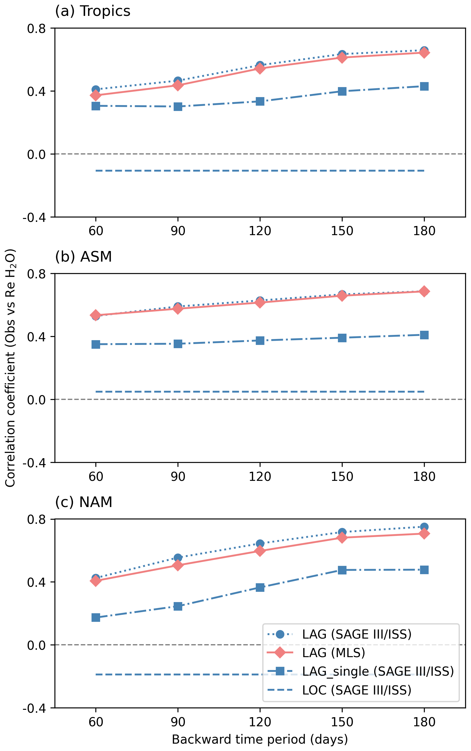
Figure 3 Correlation coefficients between observed and reconstructed water vapor mixing ratios (TST-only) for all points within 15.5–20.0 km. Panels show results for the tropics (a), ASM (b), and NAM (c). Red diamonds indicate results of experiment LAG based on MLS. Blue markers and lines indicate results based on SAGE III/ISS: dashed lines for LOC, squares for LAG_single, and circles for LAG. LOC values remain constant because they do not depend on backward time in the Lagrangian experiments.

The reconstructions from LAG show the highest correlations with observations, followed by LAG_single, while LOC shows the lowest values. As expected, using local cold point temperatures to determine stratospheric water vapor produces unreliable results (cf. Fueglistaler et al., 2005). Reconstructions using smaller trajectory ensembles (LAG_single) are less accurate than using large ensembles (LAG), as the reconstruction is sensitive to the initial air parcel position and to small variations in wind and diabatic heating rates. For the reconstructions based on MLS and SAGE III/ISS, the choice of dataset does not significantly affect performance across the three regions.

The Lagrangian reconstruction of water vapor identifies the minimum saturation mixing ratio along trajectories, making the simulation results sensitive to the backward simulation length. As shown in Fig. 3, all Lagrangian experiments display increasing correlation coefficients with longer backward periods. For example, in LAG (SAGE III/ISS), the correlation for the ASM increases from 0.53 (60 d) to 0.69 (180 d), and for the NAM from 0.43 to 0.75, with the steepest rise occurring between 60 and 120 d. The improvements in correlation indicate that UTLS water vapor mixing ratios in August are partly influenced by processes from boreal spring or even winter, particularly at higher altitudes where it needs months for air parcels to sample their LCPs. This delayed influence is consistent with the atmospheric “tape recorder”, in which anomalies imprinted at the cold point propagate upward with weak tropical upwelling (Mote et al., 1996). Within the ASM anticyclone, weak mixing preserves this memory along ascending trajectories, a process often described as “upward spiraling ascent” (Vogel et al., 2019).

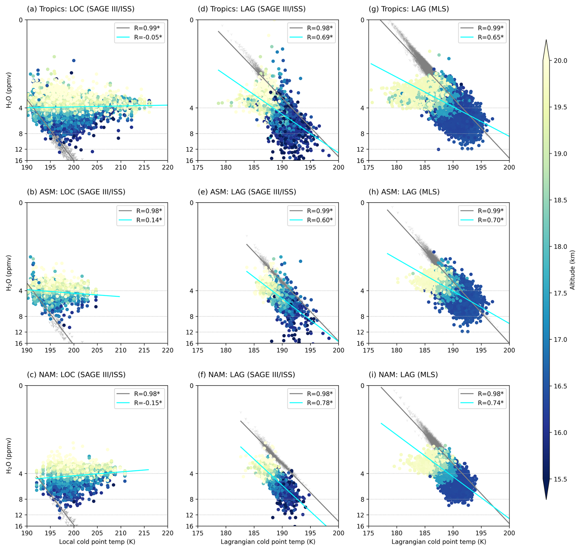
Figure 4 Scatter plots of water vapor (H₂O) mixing ratios (TST-only) versus cold point temperatures. Left: water vapor observations (SAGE III/ISS) water vapor versus local cold point temperatures (experiment LOC). Middle: water vapor observations (SAGE III/ISS) versus Lagrangian cold point temperatures (experiment LAG based on SAGE III/ISS). Right: water vapor observations (MLS) versus Lagrangian cold point temperatures (experiment LAG based on MLS). Colored points denote water vapor observations, with color indicating altitude. Grey dots represent reconstructed saturation mixing ratios. Legends give the correlation coefficients, with stars marking statistical significance at the 95 % confidence level (Student's t-test).

In general, the Lagrangian temperature history is essential for explaining dehydration near the tropical tropopause and the resulting dryness of the lower stratosphere (Fueglistaler et al., 2005). In Northern Hemisphere monsoon circulations, however, air masses are partly confined, and it remains unclear whether dehydration and moistening are governed primarily by local processes such as monsoon convection. To address this, Fig. 4 compares correlations of SAGE III/ISS and MLS water vapor in the UTLS with local cold point temperatures and with LCP temperatures.

The correlation between the observed water vapor mixing ratios and the local cold point temperatures is very weak (Fig. 4a–c), and saturation values derived from them (grey points) show large moist biases relative to observations: 13.89 ppmv in the tropics, 5.85 ppmv in the ASM, and 13.80 ppmv in the NAM. In contrast, correlations with LCP temperatures, as derived from the trajectories, are much stronger (Fig. 4e, f) and the reconstructed water vapor biases are dryer by ∼ 1–2 ppmv across all regions. These results show that, as in the tropics, UTLS water vapor in the monsoon regions correlates strongly with LCP temperatures rather than with local cold point temperatures, indicating that dehydration in these regions is primarily governed by non-local processes. However, overshooting convection – often considered a direct injection pathway for water vapor into the lower stratosphere – is a sub-grid-scale process not represented in the advection–condensation approach, which relies on large-scale fields. As a result, this method likely underestimates the impact of convection, and the weak correlation with local temperatures does not entirely rule out a role for local processes in the monsoon regions.

3.2 Dehydration regions

Figure 5 shows the spatial distribution of LCPs, and Fig. 6 presents the corresponding probability density functions (PDFs) that highlight the main dehydration regions. The left panels in Fig. 5 show results based on SAGE III/ISS. Overall, the LCPs are largely confined within the tropics. For the ASM (Fig. 5c), the LCPs cluster near the monsoon region, and show high reconstructed mixing ratios consistent with the elevated cold point temperatures. In the case of the NAM (Fig. 5e), although some LCPs are situated in its vicinity, a considerable portion is concentrated over southern Asia. The results based on MLS show similar features (Fig. 5b, d, f).

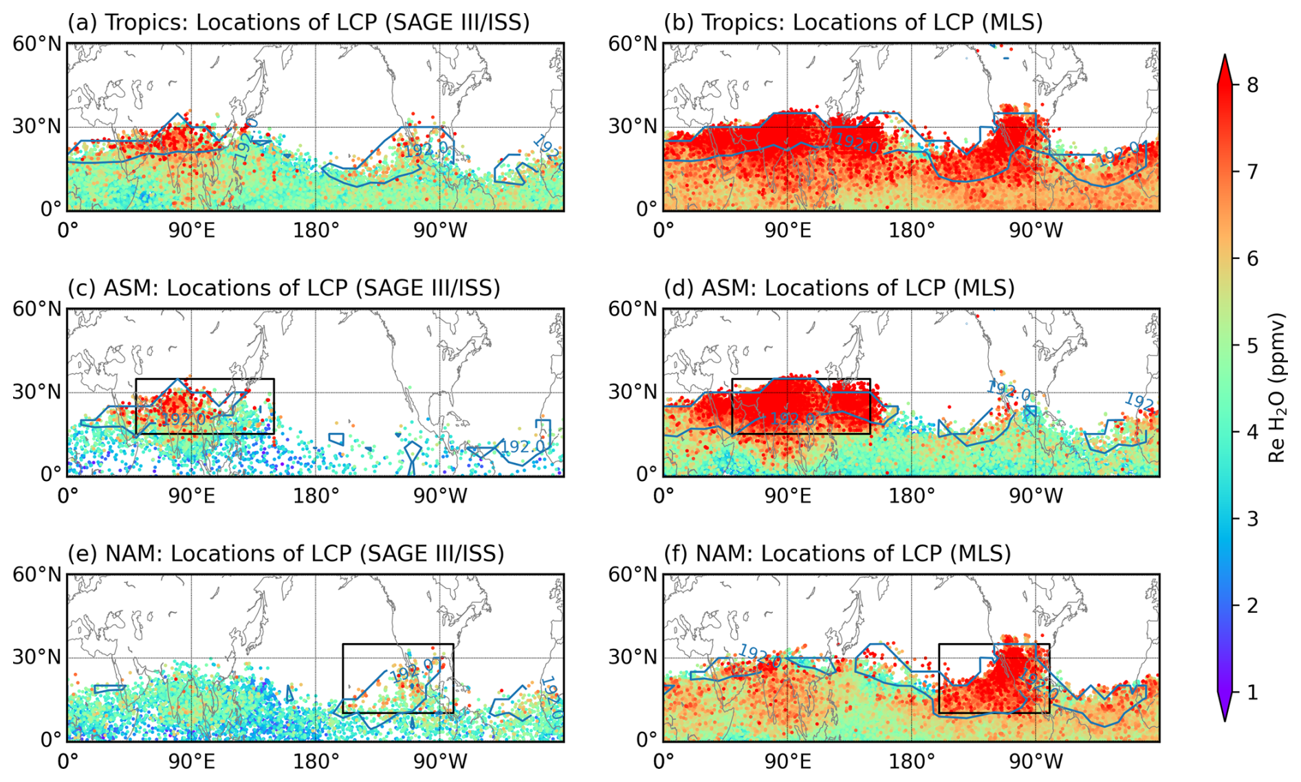
Figure 5 Horizontal distributions of Lagrangian cold point (LCP) locations used for water vapor reconstruction at 16.5 km, derived from experiment LAG (TST-only). Colors denote the reconstructed water vapor mixing ratios (Re H₂O) at the LCPs, with backward trajectories launched in the tropics (a, b), ASM (c, d), and NAM (e, f). Scatter points are plotted in ascending order of reconstructed values. Blue contours mark the 192 K cold point temperature. Left panels (a, c, e) show results based on SAGE III/ISS, and right panels (b, d, f) show results based on MLS. Black boxes indicate the regions where the backward trajectories are launched.

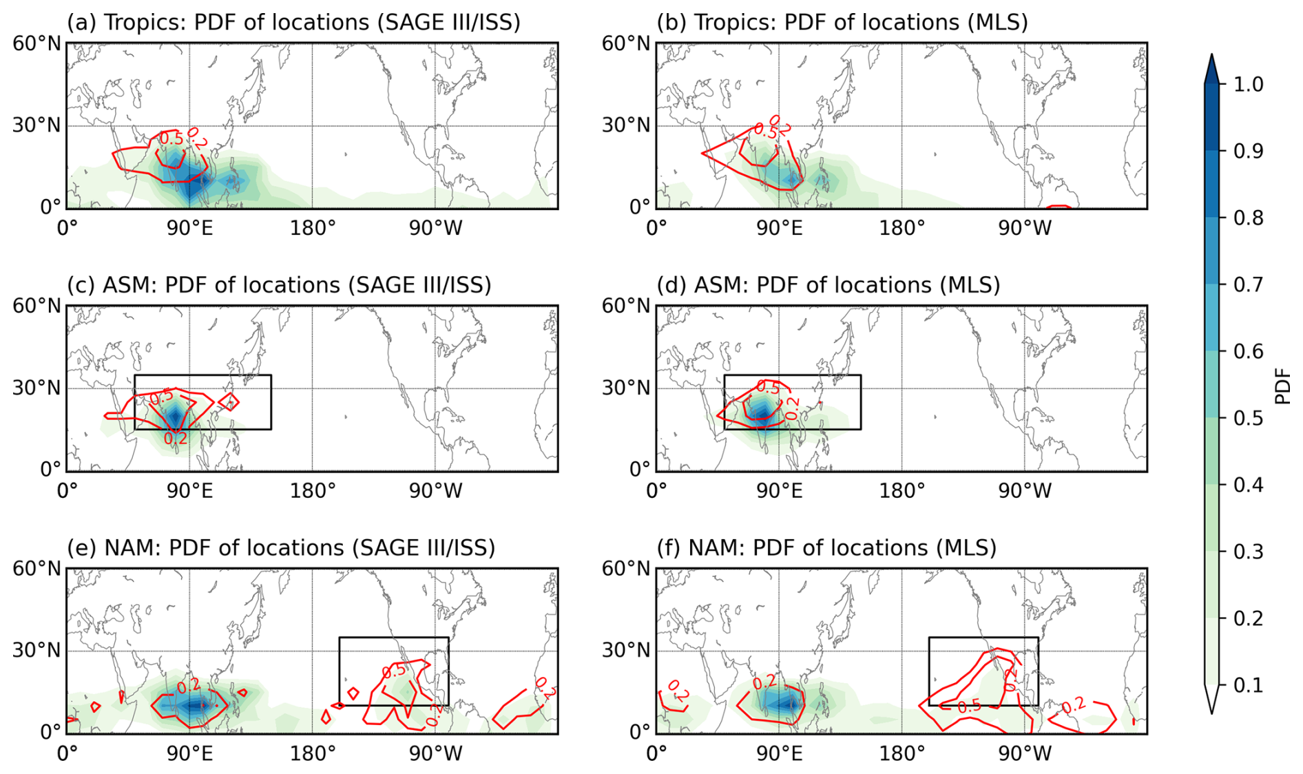
Figure 6 Probability density functions (PDFs) of the locations of Lagrangian cold points (LCPs) shown in Fig. 5. Results are presented for the entire tropics (a, b), ASM (c, d), and NAM (e, f). Red contour lines mark the PDFs of the locations with the top 10 % of reconstructed water vapor mixing ratios. Left panels (a, c, e) show results based on SAGE III/ISS, and right panels (b, d, f) show results based on MLS.

The PDFs (Fig. 6) highlight the main dehydration regions. Regardless of whether air parcels end up in the ASM, NAM, or across the tropics, southern Asia emerges as the dominant dehydration region for tropical UTLS air, similar with previous studies (Bonazzola and Haynes, 2004; Schoeberl and Dessler, 2011). Air parcels dehydrated in the ASM can then circulate within the anticyclone, ascend into the stratosphere, and contribute to enhanced lower stratospheric water vapor (Konopka et al., 2023). The red contours further show the PDFs for the top 10 % of reconstructed water vapor mixing ratios. For the ASM (Fig. 6c–d), the moistest air is primarily dehydrated locally. For the NAM (Fig. 6e–f), two dominant dehydration centers emerge: one in southern Asia and another, more pronounced, near the NAM itself. These results suggest that stratospheric air in the NAM is largely dehydrated remotely over southern Asia, while the moistest mixing ratios are shaped by both remote transport and local processes.

3.3 Lagrangian reconstruction and convection

We further examine the relation between the dry bias in the reconstructions and convection as a potential moistening process. Following recent studies (e.g., Randel et al., 2015; Peña-Ortiz et al., 2024), we use OLR as a proxy for convection, with low (high) OLR values indicating strong (weak) convection. It should be noted that, while widely applied, OLR mainly captures cold cloud tops and may miss thin convection with warm cloud tops, which can introduce regional biases (e.g., Liu et al., 2007).

Randel et al. (2015) analyzed MLS observations from May to September (2005–2013) to derive water vapor time series in the ASM UTLS (specifically at 100 hPa), and further separated wet and dry phases to reveal associated convection anomalies. They identified a west–east dipole structure in convection across the ASM, likely linked to different modes of the ASM anticyclone (Honomichl and Pan, 2020). Strong convection in the eastern part of the monsoon region (20–30° N, 80–110° E) corresponded to dry UTLS phases (low ASM water vapor), and vice versa. Building on the method used in Randel et al. (2015), we derive two OLR indices to represent convection intensity in the ASM: an OLR-West index for the western part and an OLR-East index for the eastern part (Sect. 2.2). Using these, we composite reconstructed and observed (SAGE III/ISS) UTLS water vapor mixing ratios for the ASM region (here defined as 15–35° N, 60–140° E). Days of strong and weak convection are identified as OLR temporal anomalies ≤−1.5 and $\ge +\mathrm{1.5}$ standard deviations from the mean, respectively.

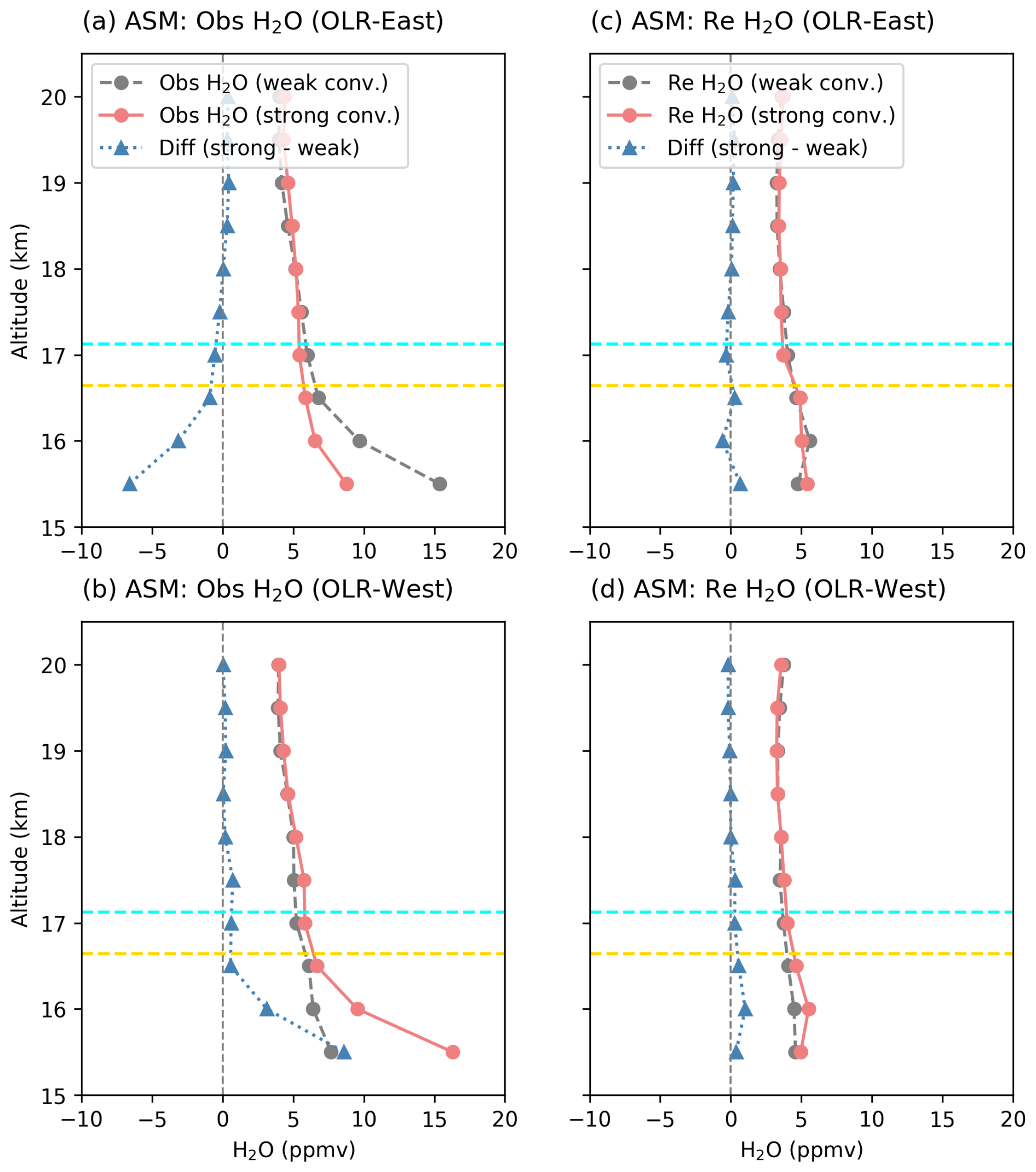
Figure 7 Vertical profiles of water vapor (H₂O) mixing ratios in the ASM region under the influence of convection, based on SAGE III/ISS. Left panels show observed profiles averaged over the 0–10 d following weak-convection (grey lines) and strong-convection (coral lines) days, along with their differences (blue lines), for OLR-West (a) and OLR-East (b) indices. Right panels show reconstructed profiles for weak- and strong-convection days, and their differences, for OLR-West (c) and OLR-East (d). As in Fig. 2, cyan and yellow dashed lines mark the climatological cold point tropopause and lapse rate tropopauses in August, respectively.

Figure 7 shows water vapor observations and reconstructions averaged over the 0–10 d following strong and weak convection days. For the eastern part of the ASM, composites indicate that observed water vapor mixing ratios are lower on strong-convection days than on weak-convection days below 17.5 km (Fig. 7a). The drying effect is weak in the lower stratosphere at 17.5 km (−0.21 ppmv) but more pronounced at 15.5 km in the troposphere (−6.6 ppmv). In contrast, composites for the western part of the ASM show the opposite pattern: water vapor mixing ratios are higher on strong-convection days than on weak-convection days below 17.5 km (Fig. 7b). These results are consistent with Randel et al. (2015), indicating that strong convection in the eastern ASM is linked to a dry UTLS, whereas a westward shift of convection is associated with a moist UTLS.

The right panels of Fig. 7 show the reconstructed water vapor profiles. Below the lapse-rate tropopause (yellow dashed lines), the reconstructions display little response to changes in convection intensity, indicating that the reconstruction method cannot capture the influence of the west–east convection shift in the ASM region. The discrepancy underscores the key limitation of the simple Lagrangian reconstruction, that it is not capable of capturing the convective moistening and drying.

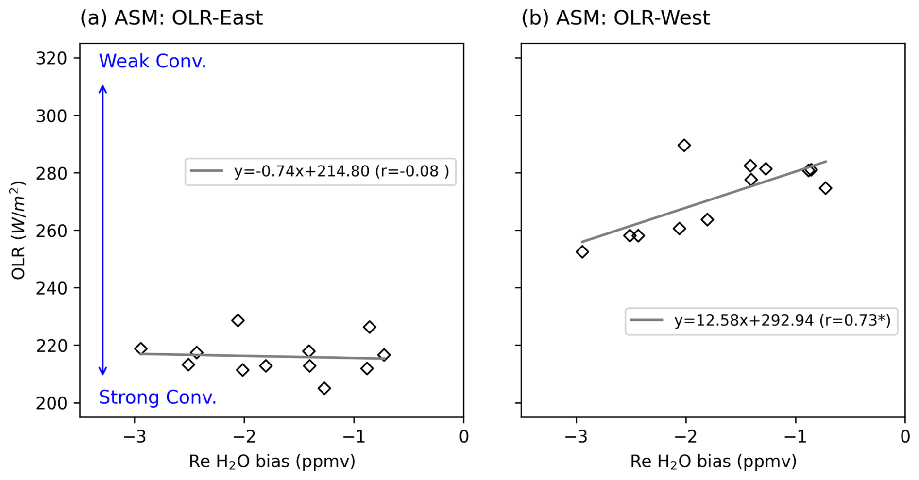
Figure 8 Scatter plots of OLR (convection intensity) versus biases in reconstructed water vapor (H₂O) mixing ratios (SAGE III/ISS) at 16.5 km for the ASM. Panels (a) and (b) show results using OLR-East and OLR-West, respectively. Biases are half-monthly averages, while OLR values are first averaged over the 0–10 d preceding each date and then half-monthly averaged. Legends show the regression line equations and correlation coefficients, with a star indicating statistical significance at the 95 % confidence level based on the Student's t-test.

Finally, we investigate potential relations between biases in the reconstruction and the intensity of convection. Figure 8a and b show the correlation between reconstruction biases near the lapse rate tropopause (16.5 km) and the convection intensity in the eastern and western ASM, respectively. Convection is stronger in the eastern ASM (OLR 200–230 W m²) than in the western ASM (OLR 240–280 W m²), but it shows no significant correlation with the reconstruction bias (Fig. 8a). In contrast, convection in the western ASM is strongly correlated with the reconstruction bias ($r={\mathrm{0.73}}^{*}$, statistically significant at the 95 % confidence level; Fig. 8b), indicating that dry biases increase following strong-convection periods in the western ASM. Therefore, the moistening effect of convection in the western part of the monsoon region (e.g. related to ice injection), which is not included in the simple trajectory reconstruction approach, likely contributes strongly to the reconstruction dry bias. The correlation between the dry biases and the convection intensity in the western ASM decreases with altitude, with coefficients of 0.73^*, 0.46, and 0.24 at 16.5, 17.0, and 17.5 km, respectively. Except at 16.5 km, correlations are not statistically significant at the 95 % confidence level. The strong correlation at 16.5 km suggests that convection particularly affects the water vapor mixing ratios near the tropopause, whereas above 17.0 km, the water vapor mixing ratios become less sensitive to convection and are more strongly governed by large-scale transport processes.

4 Discussion

As shown in Figs. 1 and 2, the reconstruction exhibits a consistent dry bias of about 1.5 ppmv above the cold point tropopause in the tropics. A similar bias was reported by Liu et al. (2010), who suggested that including cloud microphysical processes could alleviate this bias. Schoeberl and Dessler (2011) implemented a Lagrangian model that allows a certain degree of supersaturation, and achieved close agreement with MLS observations. Other studies have also demonstrated that allowing for supersaturation at LCPs can reduce the dry bias (Schiller et al., 2009; Ploeger et al., 2011). While effective, such methods remain simplified treatments of the complex microphysical processes that govern dehydration efficiency, as well as of other small-scale influences such as turbulence and mixing (Poshyvailo et al., 2018). These underrepresented processes likely contribute to the dry bias in our reconstruction.

While the simplified Lagrangian method performs well in reconstructing the moisture enhancement in the ASM, it struggles to represent the moisture budget in the NAM, suggesting that different mechanisms are at play in this region. Previous studies indicate that during boreal summer, the ASM is characterized by a strong anticyclonic circulation at 100 hPa, accompanied by a smaller, roughly symmetric anticyclone in the Southern Hemisphere subtropics. These monsoon circulation patterns are consistent with the dynamical structure of the Gill response (Park et al., 2007). In contrast, geopotential height fields over North America at 100 hPa show no such structure, underscoring a fundamental difference between the NAM and ASM from a large-scale circulation perspective. Furthermore, studies by Smith et al. (2017) and O'Neill et al. (2021) demonstrate that particularly intense deep convection events over North America can transport water vapor and ice directly into the lower stratosphere. These results suggest that deep, possibly overshooting convection plays a more critical role in the UTLS water vapor budget in the NAM than in other regions, and may be the primary cause of the large biases observed in Lagrangian reconstructions. Additionally, our trajectory simulations suggest that long-range transport from southern Asia to the NAM region significantly influences water vapor mixing ratios in the NAM region, making the reconstructed values sensitive to uncertainties in ERA5 temperatures, winds and diabatic heating rates. The coexistence of multiple, competing mechanisms within convection events (Homeyer et al., 2024) further adds substantial complexity to representing long-range transport in models. These uncertainties make it difficult to accurately reproduce water vapor mixing ratios over the NAM.

Previous studies have shown that trajectories computed with 6-hourly reanalysis data exhibit transport errors and warm biases around the cold point tropopause compared to trajectories calculated with higher temporal resolution (1-hourly) data (Pisso et al., 2010; Bourguet and Linz, 2022). Such biases can affect the simulation of dehydration processes and, in turn, the reconstructed water vapor distribution. Incorporating additional tracers originating from Asia could help to evaluate whether long-range transport to the NAM region and its remote influence on NAM water vapor are accurately represented in current trajectory-based reconstructions.

5 Conclusions

This study investigates the UTLS water vapor in monsoon regions over Asia and North America durgin boreal summer based on SAGE III/ISS and MLS, and particularly assesses the performance of related Lagrangian reconstruction approaches. The results show that the Lagrangian reconstructions consistently exhibit a dry bias of about 1.5 ppmv across the tropics. Despite this, the method reproduces UTLS water vapor variations and structures well in the ASM, but performs poorly in the NAM. Reconstruction skill improves with altitude above the tropopause. Also, larger trajectory ensembles give more robust results than smaller ensembles.

In the ASM, UTLS water vapor mixing ratios are primarily controlled by local tropopause temperatures over southern Asia. In the NAM, water vapor is strongly influenced by long-range transport from southern Asia and hence by tropopause temperatures in that region. However, the moistest air masses appear to be locally controlled by temperatures in the NAM region.

We hypothesize that the failure of the water vapor reconstruction in the NAM UTLS arises primarily from an underestimation of local moistening processes such as deep convection and ice injection, which are not explicitly included in the reconstruction framework. Errors in representing cross-Pacific long-range transport likely contribute further to the particularly large dry bias in the NAM reconstructions.

Using outgoing longwave radiation as a proxy for convection, we also assessed the impact of convection on UTLS water vapor variability and on biases in the Lagrangian reconstructions. Observations from SAGE III/ISS confirm the findings of Randel et al. (2015), showing that strong convection in the eastern ASM leads to UTLS drying, whereas a westward shift of convection results in UTLS moistening. These signals, however, are not captured by the reconstructions. Correlation analyses demonstrate that the Lagrangian reconstructions have larger dry biases when convection intensity increases in the western part of the ASM region. These findings suggest that underestimated moistening from convection in the western part of the ASM is a key driver of the dry bias in the reconstructions.