Estimating surface sulfur dioxide concentrations from satellite data over eastern China: Using chemical transport models vs. machine learning

Sulfur dioxide (SO₂) is an important air pollutant that contributes to negative health effects, acid rain, and aerosol formation and growth. SO₂ has been measured using ground-based air quality monitoring networks, but routine monitoring sites are predominantly in urban areas, leaving large gaps in the network in less populated locations. Previous studies have used chemical transport models (CTMs) or machine learning (ML) techniques to estimate surface SO₂ concentrations from satellite vertical column densities, but their performance has never been directly compared. In this study, we estimated surface SO₂ concentrations using Ozone Monitoring Instrument (OMI) retrievals over eastern China from 2015–2018 utilizing GEOS-Chem CTM simulations and an extreme gradient boosting ML model. For the first time, we quantified methodological uncertainties for both methods and directly compared their performance on the same truth dataset. The surface concentrations estimated from the CTM-based method had similar spatial distributions (r=0.58) and temporal variations compared to the in situ measurements but were underestimated (slope = 0.24; RPE = 75 %) and had worsening performance over time. The ML-based method produced more accurate spatial distributions (r = 0.77) and temporal variations with a smaller discrepancy (slope = 0.69; RPE = 30 %) and stable performance over time. Despite the higher accuracy of the ML-based method at the monitoring sites, the CTM-based method produced more reasonable gridded spatial distributions over areas without monitoring data. These results suggest that satellite data could be a reliable way to estimate global SO₂ concentrations to parameterize other chemical processes in the atmosphere.

1 Introduction

Sulfur dioxide (SO₂) is an important air pollutant due to its effects on human health, air quality, weather, and climate. SO₂ has many anthropogenic sources such as fossil fuel combustion in power plants and ore smelters, as well as natural sources from volcanoes (Engdahl, 1973). Surface SO₂ concentrations are mainly driven by anthropogenic activity in urban areas and are known to negatively impact cardiovascular and respiratory health (Engdahl, 1973; Krzyzanowski and Wojtyniak, 1982). SO₂ also readily undergoes oxidation reactions in the atmosphere to form sulfuric acid, which further contributes to acid rain (Seinfeld and Pandis, 2016) and participates in aerosol formation and growth (Lee et al., 2019). These aerosols can then additionally affect weather and the global energy budget (NASEM, 2016).

Concentrations of SO₂ at the surface have been regularly measured using ground-based air quality monitoring networks. Surface concentrations are typically measured on hourly to daily time intervals, but the sites are predominantly located in urban areas, leaving large gaps in the network elsewhere. In addition to surface-based air quality monitors, satellite-based instruments can measure total-column concentrations of SO₂ globally from space. These SO₂ vertical column densities (VCDs) are retrieved using the absorption of backscattered solar radiation in the ultraviolet wavelengths measured by a spectrometer (e.g., Krotkov et al., 2008; Levelt et al., 2006; Li et al., 2013, 2020a; Nowlan et al., 2011; Theys et al., 2015). The VCDs are typically available over large areas in cloud-free locations on a daily basis but do not directly provide the concentrations at the surface. Additional analysis is required to estimate the surface concentrations from the satellite-retrieved VCDs.

Chemical transport models (CTMs) can be used to convert satellite VCDs into surface concentrations using simulated surface-to-VCD ratios (SVRs). This method was initially developed for estimating surface concentrations of particulate matter from satellite-based aerosol optical depth retrievals (Liu et al., 2004) and was later applied to nitrogen dioxide (NO₂; Lamsal et al., 2008) and SO₂ (Lee et al., 2011). Lee et al. (2011) and Zhang et al. (2021) each used coarse-resolution CTMs (grid spacings on the order of 100 km) to convert SO₂ VCDs from the Ozone Monitoring Instrument (OMI) into surface concentrations over North America for 2006, and China for 2005–2018, respectively. McLinden et al. (2014) and Kharol et al. (2017) used higher-resolution CTMs (grid spacing on the order of 10 km) and OMI SO₂ VCDs to estimate the surface concentrations over the Canadian oil sands from 2005–2011, and the North American continent from 2005–2015, respectively. These four studies each demonstrated that annual mean satellite-derived surface SO₂ concentrations can accurately capture the spatial distribution of ground-based air quality monitoring networks, although the estimated surface concentrations were generally underestimated. An advantage of the CTM-based method is that it is based on fundamental principles of atmospheric dynamics and chemistry and can produce results that are independent of observed surface concentrations. The main limitations of CTMs are the computational expense of running the simulations (Fan et al., 2022) and relatively coarse resolution, which may lead to large biases in the representation of emissions, meteorology, and chemical processes (Wang et al., 2020a, b).

More recently, machine learning (ML) techniques have been used to estimate surface SO₂ concentrations from satellite retrievals, meteorology, and other geographic variables such as emission inventories. Zhang et al. (2022) used a Light Gradient Boosting Machine (LightGBM) to estimate surface SO₂ concentrations over northern China using OMI SO₂ VCDs, meteorological variables, emissions, land use classifications, population density, and others. Yang et al. (2023a) used radiances from the Geostationary Environment Monitoring Spectrometer (GEMS) satellite to estimate the surface concentrations of SO₂ and other criteria air pollutants in a multi-output random forest model. Both studies showed that ML techniques can accurately capture the spatial distribution and magnitude of the surface concentrations but may have artificial biases due to nonphysical links between predictors and the observed surface concentrations, such as interactions between land use classifications and skin temperature as shown by Zhang et al. (2022). In these studies, the ML models incorporated spatial (e.g., longitude, latitude, population density) and temporal (e.g., numeric day of year, hour of day) proxies to improve performance rather than depending only on measurable quantities, but this limits the physical usefulness, interpretability, and applicability of the model (Zhang et al., 2022; Yang et al., 2023a, b). An advantage of the ML-based method is that the models are typically much faster to train and run than a full CTM simulation and can utilize higher spatial and temporal resolution data (Fan et al., 2022); however, since ML models can only use statistical relationships to make predictions, they are often limited in their physical interpretability and may make their predictions based on predictors that have no physical relevance to the estimated surface concentrations.

Although the CTM- and ML-based methods have each been used to estimate surface SO₂ concentrations from satellite retrievals, there is a lack of direct comparisons between them. Here, we estimated surface SO₂ concentrations using OMI SO₂ VCDs over eastern China (105–125° E, 25–45° N) from 2015–2018 to directly compare the two methods. First, we quantified methodological uncertainties for each method for the first time. Next, we used simulated SVRs from the GEOS-Chem model to estimate the surface SO₂ concentrations from OMI using the CTM-based method. Then, we used a ML model to predict surface SO₂ concentrations from OMI VCDs, meteorological variables, and an emission inventory, which are all physically relevant to the spatial distribution or lifetime of SO₂. The results from each method were validated against ground-based in situ measurements from the China National Environmental Monitoring Centre (CNEMC) air quality monitoring network on annual and seasonal mean timescales. Finally, we compared the performance of each method on the same truth dataset over the same times and locations to gain insights on their abilities and limitations to accurately estimate the surface SO₂ concentrations from satellite data.

2 Data and methods

2.1 Study region

Eastern China has abundant anthropogenic SO₂ emissions and thus is a region with elevated surface concentrations. Satellite SO₂ retrievals typically have a low signal-to-noise ratio due to interfering absorbers (Li et al., 2020a), so regions with large SO₂ emissions and pollution, such as eastern China, are required to obtain sufficient signals from the spectrometer and provide more reliable retrievals compared to less polluted regions. A map of our study region including the locations of OMI-derived SO₂ emission sources (Fioletov et al., 2022, 2023) and CNEMC monitoring sites is shown in Fig. 1. The main sources of SO₂ in the study region include around 70 power plants, five ore smelters, and one area of oil and gas production (Fig. 1b). There are also approximately 1000 air quality monitoring stations located in the study region that were used to validate the estimated surface concentrations (Fig. 1c). Our analysis covers the period from 2015 (the first full year of in situ measurements) to 2018 (to avoid the impacts of the COVID-19 lockdowns).

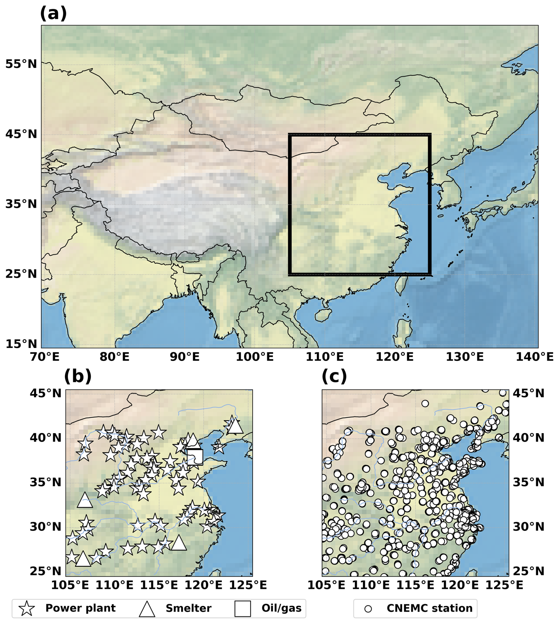
Figure 1 Maps showing the (a) study region (box; 105–125° E, 25–45° N) relative to the rest of the Asian continent, (b) locations of large SO₂ sources from the 2015 OMI emission catalogue (Fioletov et al., 2022) including 70 power plants (stars), five ore smelters (triangles), and one area of oil and gas production (square), and (c) locations of the CNEMC monitoring stations (circles).

2.2 OMI satellite data

We employed data from the Ozone Monitoring Instrument (OMI; Levelt et al., 2006), a hyperspectral ultraviolet/visible nadir solar backscatter spectrometer launched onboard the Aura satellite in 2004. Aura flies in a sun-synchronous polar orbit, and OMI is used to retrieve SO₂ VCDs with daily global coverage and a spatial resolution of 13 km × 24 km at nadir, a significant improvement from previous satellite-based instruments. The VCDs were gridded to a horizontal resolution of 0.25° × 0.25° to decrease noise in the SO₂ retrieval without significantly coarsening it from the native measurement resolution. The OMI overpass time of our study region ranged from approximately 12:15 p.m. to 02:45 p.m. local time. For both the CTM- and ML-based methods, we used the OMI Planetary Boundary Layer (PBL) SO₂ product to estimate the surface concentrations due to its main application for anthropogenic, near-surface SO₂ (Krotkov et al., 2014; Li et al., 2020b). The OMI retrievals use a principal component analysis- (PCA) based algorithm for spectral fitting based on the radiances for each row in the measurement swath with wavelengths between 310.5–340 nm (Li et al., 2013, 2020a). This version of the PCA retrievals include pixel-specific air mass factor calculations to convert slant column densities (SCDs) to VCDs rather than using a fixed value worldwide (Li et al., 2020a). The VCDs express the number of SO₂ molecules in the column and are reported in Dobson Units (DU; 1 DU = 2.69 × 10¹⁶ molecules cm⁻²). To ensure good data quality, we screened out measurements with cloud fractions greater than 0.3, solar zenith angles greater than 65°, located in the outer ten cross-track positions, or affected by the row anomaly (NASA, 2020). We also excluded extreme outliers that fell outside of five standard deviations from the mean as thresholds less than this appeared to remove legitimate data.

2.3 CNEMC ground-based monitoring data

Ground-based SO₂ concentrations from the China National Environmental Monitoring Centre (CNEMC) air quality monitoring network (CNEMC, 2024) were used to validate the performance of both the CTM- and ML-based methods. The concentrations were converted from µg m⁻³ to parts per billion (ppbv) following the procedure outlined in Wei et al. (2023). To ensure the ground-based measurements were temporally aligned with the OMI overpass, we averaged the hourly concentrations from 12:00 p.m. to 03:00 p.m. local time on days where there was at least one OMI observation within 40 km of the station. Like the OMI data, we also removed data that fell more than five standard deviations outside of the mean.

2.4 CTM-based technique

We used simulated SVRs from the GEOS-Chem model (version 14.2.2; The International GEOS-Chem User Community, 2023) to convert the OMI VCDs into surface concentrations for the CTM-based method. We ran simulations for January, April, July, and October 2015. Each simulation was conducted with a one-month spin-up following Kharol et al. (2015). To reduce the computational expense, we used the monthly average SVR from each simulation to estimate the daily surface concentrations within the corresponding winter (DJF), spring (MAM), summer (JJA), and autumn (SON) months (referred hereafter as quasi-seasonal temporal sampling) for all years of the study period. The model was run at a horizontal resolution of 2.5° (longitude) × 2.0° (latitude) with 47 vertical layers and was driven by assimilated GEOS-FP meteorology (Lucchesi, 2018) and the Community Emissions Data System (CEDS) anthropogenic emission inventory (Hoesly et al., 2018). The internal time steps for the chemistry and advection calculations in the model were lengthened by 50 % from the default values to reduce simulation times while minimizing errors following Philip et al. (2016). Despite the longer internal timesteps, the Courant-Friedrichs-Lewy condition is maintained with a Courant number of 0.041, indicating numerical stability of the simulations. The surface concentrations were assumed to be equal to the concentrations at the lowest model level (∼ 60 m above ground level). The output timestep of GEOS-Chem was every three hours, so it was sampled at 02:00 p.m. local time, which is the only output inside the OMI overpass window. We only included GEOS-Chem data in the analysis if there was at least one valid OMI observation within the model grid cell on a given day.

The approach from Lee et al. (2011) was used to infer surface SO₂ concentrations from OMI VCDs and simulated vertical SO₂ profiles from GEOS-Chem (GC). Lee et al. (2011) showed that the CTM-based method provided accurate results even with CTM resolutions that are much coarser than the satellite data. The monthly averaged profiles and SVRs from GEOS-Chem are shown in Fig. S1 in the Supplement. The profiles indicate that most of the SO₂ within the vertical column is located near the surface and within the boundary layer (Fig. S1). The concentrations then drop to near zero in the free troposphere and have small variations, indicating a lack of elevated SO₂ plumes (Fig. S1). The profiles from the GEOS-Chem simulations are similar to those from aircraft observations (e.g., Li et al., 2012; Norman et al., 2025; Shan et al., 2025; Xue et al., 2010) and higher resolution simulations (Norman et al., 2025) over China. The surface SO₂ concentrations for the CTM-based method (S_OMI) were calculated on a daily basis at 0.25° × 0.25° resolution using the daily OMI VCDs and averaged GEOS-Chem SVRs from the model grid cell that the OMI measurement lies within using Eq. (1):

$$\begin{array}{}\text{(1)}& S_{\mathrm{OMI}}={\displaystyle \frac{\mathit{\nu }{S}_{\mathrm{GC}}}{\mathit{\nu }{\mathrm{\Omega }}_{\mathrm{GC},\mathrm{PBL}}+{\mathrm{\Omega }}_{\mathrm{GC},\mathrm{FT}}}}\times {\mathrm{\Omega }}_{\mathrm{OMI}},\end{array}$$

where S is the surface SO₂ concentration in ppbv and Ω is the SO₂ VCD in DU. The FT and PBL subscripts are the free-tropospheric and boundary layer VCDs, respectively, which were calculated relative to the GEOS-FP PBL height. Since there is a significant difference in horizontal resolution between the satellite and model data, OMI VCDs were used to provide sub-model grid variability (ν) using Eq. (2):

$$\begin{array}{}\text{(2)}& \mathit{\nu }={\displaystyle \frac{{\mathrm{\Omega }}_{\mathrm{OMI}}}{{{\mathrm{\Omega }}^{\prime }}_{\mathrm{OMI}}}},\end{array}$$

where Ω_OMI is the OMI VCD at 0.25° × 0.25° resolution and ${\mathrm{\Omega }}_{\mathrm{OMI}}^{\prime }$ is the average OMI VCD over the 2.5° × 2.0° GEOS-Chem grid cell. To compare the estimated surface concentrations to the in situ surface monitoring data, we used a 40 km averaging radius around each station to increase the amount of usable data and further reduce the noise in the OMI data. This is similar to previous studies (i.e., Kharol et al., 2017) and maximizes both the slope and correlation compared to other radii, as shown in Fig. S2. In Sect. 3.1, the surface concentrations estimated from the CTM-based method will be validated against the in situ measurements on the full four years of data since an independent testing dataset is not required for this method. Then, the CTM-derived concentrations will be resampled to match the independent testing dataset to directly compare to the performance of the ML-derived concentrations in Sect. 4.

Since only simulations for January, April, July, and October 2015 were available to provide SVRs, there are two inherent assumptions regarding the temporal representativeness of the SVRs. The first assumption was using quasi-seasonal temporal sampling for the SVRs and calculating the estimated surface concentrations. To test the impact of temporal representativeness on the estimated surface concentrations, we ran an additional GEOS-Chem simulation to cover all of spring (MAM) 2015. We also employed a full year of archived 2018 GEOS-CF data (NASA GMAO, 2025), which has improved temporal (hourly) and spatial (0.25° × 0.25°) resolution compared to GEOS-Chem and uses the same chemistry module, so they tend to produce similar results (Keller et al., 2021). We found that the intraseasonal variability in the SVR was 0.6 ppbv DU⁻¹ for MAM in both GEOS-Chem and GEOS-CF, as shown by Fig. S3. Therefore, we used the GEOS-CF data to estimate this uncertainty for the entire year. We found that the average intraseasonal variability in the SVRs for the full year was 0.8 ppbv DU⁻¹ (Fig. S3). We also used the full year of GEOS-CF data to test the impact of temporal representativeness on the annual mean surface SO₂ concentrations. Figure S4b–f show that there was no significant difference in the accuracy of the annual average surface SO₂ concentrations among the different temporal sampling techniques ranging from daily to annual mean SVRs. The slopes and correlations of the surface concentrations were consistent only ranging between 0.23–0.29 and 0.33–0.40, respectively (Fig. S4b–f). The sensitivity analysis with GEOS-CF also suggested that improving the spatial resolution of the CTM while maintaining the same temporal sampling of the SVRs did not have a large impact on the accuracy of the estimated surface concentrations despite an improvement in spatial resolution by nearly a factor a 10, as indicated by Fig. S4a and d for 2018 data, as well as Fig. S5 for all years of the study period.

The other assumption was only using a single year of simulations to convert four years of OMI data into surface concentrations. Kharol et al. (2017) did not have simulations that spanned their entire analysis period, but the implications of this were never discussed. To address this, we first compared the monthly averaged SVRs from observations (calculated using CNEMC surface concentrations and OMI VCDs) for each year in the study period to the 2015 GEOS-Chem simulations to ensure there is no significant changes over time. Figure S6 shows boxplots of the observed and GEOS-Chem SVRs with the percent difference between them. In general, the differences between the observed and GEOS-Chem SVRs were consistent across all years of the study period, typically ranging from 73 %–89 % (Fig. S6). We also ran additional GEOS-Chem simulations for January, April, July, and October 2018 to assess if the simulated SVRs change over time. Boxplots for these two sets of simulations can be seen in Fig. S7 and indicate that the GEOS-Chem SVRs only changed by 0.8 ppbv DU⁻¹, or 9 %, from 2015 to 2018. The implications of these uncertainties on the resultant concentrations are discussed further in Sect. 2.6.

2.5 ML-based technique

To estimate the surface SO₂ concentrations using a ML model, we used an eXtreme Gradient Boosting regression model (XGBoost; Chen and Guestrin, 2016) to statistically relate satellite-based SO₂ VCDs, meteorological variables, and emissions data to the in situ measurements. XGBoost models use a scalable tree boosting system to efficiently train an ensemble of decision trees by adding a new tree with each training epoch and learning with each iteration (Chen and Guestrin, 2016; Friedman, 2001). Previous studies have shown that XGBoost and LightGBM models are able to estimate surface concentrations from satellite data more effectively than other ML architectures as shown by Kang et al. (2021) and Zhang et al. (2022). We trained our XGBoost model with an ensemble of 500 trees, a maximum tree depth of 15 splits, and a learning rate of 0.15 on a mean squared error loss function. Neither a larger ensemble nor deeper trees improved the performance of the model, as shown by Figs. S8 and S9, respectively.

Our ML model was trained on a small number of variables (five) that each have known physical relationships to the spatial distribution or lifetime of atmospheric SO₂. By using a small number of variables, it is easier to derive physical meaning from the ML predictions without sacrificing accuracy since the input variables are already known to affect surface SO₂ concentrations. We used daily OMI SO₂ VCDs to estimate the spatial distribution of SO₂, hourly European Centre for Medium-Range Weather Forecasts (ECMWF) Reanalysis v5 (ERA5; Hersbach et al., 2020; ECMWF, 2019) 100 m u-winds, 100 m v-winds, and boundary layer heights averaged over the OMI overpass window were used to account for the meteorological mixing and dispersion of SO₂, and monthly SO₂ emissions from the CEDS inventory to capture the locations of SO₂ sources. The ERA5 meteorological variables were provided at 0.25° × 0.25° horizontal resolution, and the CEDS emissions were provided at 0.5° × 0.5° horizontal resolution. We trained the model on logarithmic boundary layer heights to get better sensitivity to variations in low boundary layers, and logarithmic emissions since the values ranged several orders of magnitude. The model is summarized in Eq. (3) as:

$$\begin{array}{}\text{(3)}& \begin{array}{rl}{S}_{\mathrm{ML}}& =\text{XGBoost}\left({\mathrm{\Omega }}_{\mathrm{OMI}},U_{\mathrm{ERA}\mathrm{5}},V_{\mathrm{ERA}\mathrm{5}},\right.\\ & \left.{\log }_{\mathrm{10}}\left[{\mathrm{PBLH}}_{\mathrm{ERA}\mathrm{5}}\right],{\log }_{\mathrm{10}}\left[E_{\mathrm{CEDS}}\right]\right),\end{array}\end{array}$$

where S_ML is the predicted surface concentrations from the XGBoost ML model, Ω_OMI is the satellite SO₂ VCD, U_ERA5 is the u-wind, V_ERA5 is the v-wind, PBLH_ERA5 is the boundary layer height, and E_CEDS is the SO₂ emissions. Earlier versions of the model were trained on 11 predictors, but the predicted surface concentrations produced an unrealistic spatial distribution of SO₂, as shown in Fig. S10. Additionally, some of the predictors were shown to be relatively unimportant to the model output, as indicated by the permutation importance in Fig. S11. The reduction of predictors from 11 down to five led to an improvement in the statistical performance and spatial distribution of the estimated surface concentrations, suggesting that utilizing known physical relationships between variables is more beneficial than the number of predictors in a ML model.

We trained the model on 90 % of the daily data (N = 137 630) from 2015–2018 with ERA5 and CEDS predictors sampled to match the valid OMI observations. The input variables were sampled and averaged within 40 km of the CNEMC sites for training, as done in the CTM-based method, and the predicted surface concentrations from the XGBoost model are provided at each CNEMC site in the dataset. The remaining 10 % of the data (N = 15 292) was reserved for a sample-based independent validation. This split of the training and independent testing datasets was used by previous studies (e.g., Zhang et al., 2022; Yang et al., 2023a, b) and was shown to have the best performance for the independent testing dataset for our model as shown in Fig. S12. Figure 2 shows that the model had noticeably better performance with the training data (slope = 0.89; r = 0.95) compared to the testing data (slope = 0.67; r = 0.76), indicating that the model has good performance, but is slightly overfitting, a common artifact of complex machine learning models such as XGBoost. While the model was trained to estimate the surface SO₂ concentration at each CNEMC station, the trained model can then be used to make predictions on gridded input data to obtain estimates of the surface SO₂ concentrations on a continuous domain at the same horizontal resolution as the inputs.

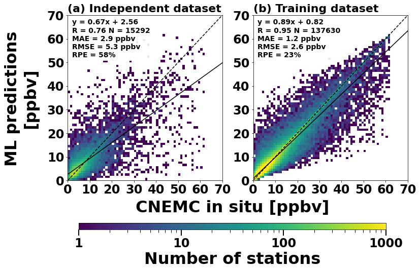
Figure 2 Scatterplots between the daily ML model predictions and CNEMC in situ measurements for the (a) independent dataset and (b) training dataset. Scatterplots are binned every 1 ppbv. Each scatterplot is colored by the number of stations in each bin and includes a linear regression analysis with the best fit line (solid line), best-fit equation, correlation coefficient, total number of stations, 1:1 line (black dashed line), MAE, RMSE, and RPE.

2.6 Methodological uncertainties

This study provides the first detailed discussion of the individual sources and summation of uncertainties for either methodology. To estimate the uncertainty of the input variables for both methods, we performed moving-block bootstrapping (Flyvbjerg and Petersen, 1989) with 10 000 iterations on the daily gridded data. For each bootstrap, a horizontal coordinate and date was randomly sampled with replacement. For each random sample, a temporal block of five days in each direction from the randomly sampled day was used to calculate the standard deviation. After all bootstraps were completed, the uncertainty was defined as the average of the standard deviations calculated from each iteration. This was done for the OMI SO₂ VCDs, GEOS-Chem SVRs, and ERA5 meteorology. The uncertainty in the CEDS emission inventory was not included due to the monthly temporal resolution, and a lack of uncertainty quantification in previous literature (e.g., Hoesly et al., 2018; McDuffie et al., 2020).

For the CTM-based method, the summation of error was determined using error propagation. For the error propagation, Eq. (1) was simplified such that:

$$\begin{array}{}\text{(4)}& S_{\mathrm{OMI}}=\left({\mathrm{SVR}}_{\mathrm{GC}}\right)\times {\mathrm{\Omega }}_{\mathrm{OMI}},\end{array}$$

where SVR_GC is the monthly averaged SVR from the GEOS-Chem simulations. Equation (4) was used in the error propagation formula to obtain Eq. (5):

$$\begin{array}{}\text{(5)}& {\mathit{\sigma }}_{S_{\mathrm{OMI}}}=\sqrt{{\mathit{\sigma }}_{{\mathrm{SVR}}_{\mathrm{GC}}}^{\mathrm{2}}{\left({\mathrm{\Omega }}_{\mathrm{OMI}}\right)}^{\mathrm{2}}+{\mathit{\sigma }}_{{\mathrm{\Omega }}_{\mathrm{OMI}}}^{\mathrm{2}}{\left({\mathrm{SVR}}_{\mathrm{GC}}\right)}^{\mathrm{2}}}\end{array}$$

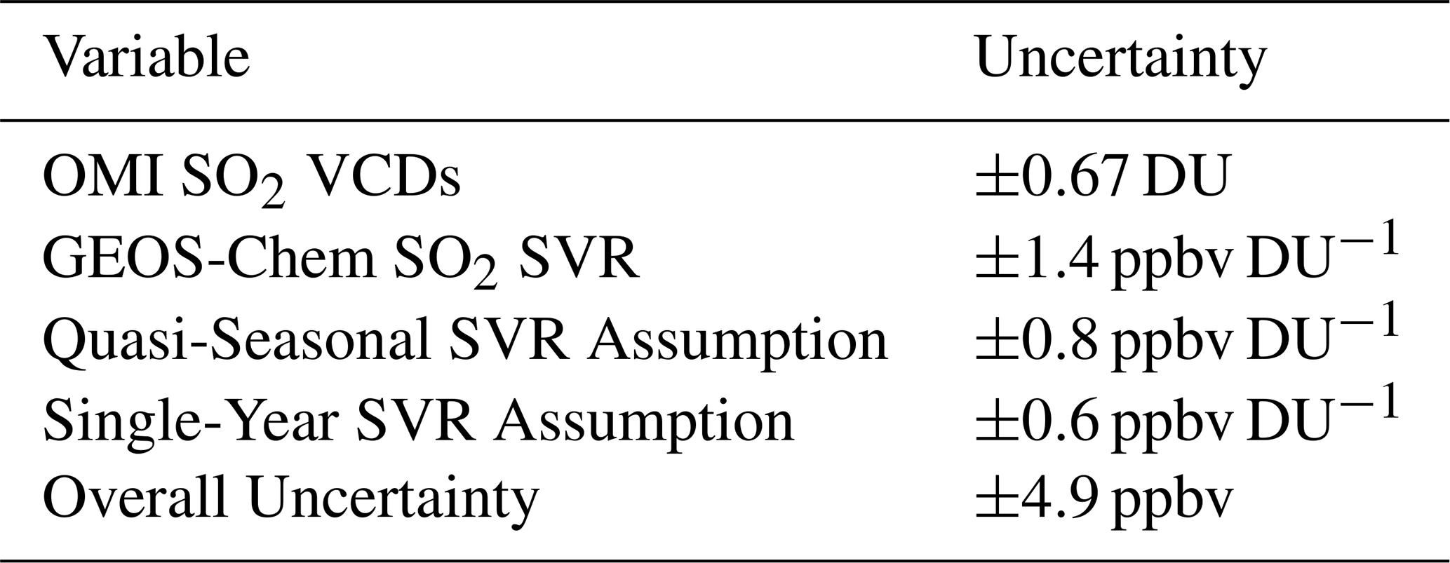
where ${\mathit{\sigma }}_{S_{\mathrm{OMI}}}$ is the propagated error of the CTM-derived concentration, ${\mathit{\sigma }}_{{\mathrm{SVR}}_{\mathrm{GC}}}$ is the uncertainty in the GEOS-Chem SVR, and ${\mathit{\sigma }}_{{\mathrm{\Omega }}_{\mathrm{OMI}}}$ is the uncertainty in the OMI SO₂ VCD. The uncertainty in the GEOS-Chem SVR was initially calculated with bootstrapping, but also needs to account for the uncertainties of the quasi-seasonal and single-year assumptions in the CTM-based methodology. The quasi-seasonal and single-year assumptions were defined and quantified in Sect. 2.4. These three sources of GEOS-Chem SVR uncertainty were assumed to be independent of each other and were combined using the sum of the squares of each term. The results of the bootstrapping and error propagation are shown in Table 1. Ultimately, the methodological uncertainty of the CTM-based method is ±4.9 ppbv when considering the uncertainties of the OMI SO₂ VCDs (±0.67 ppbv DU⁻¹) and GEOS-Chem SVRs (±1.7 ppbv DU⁻¹). The OMI SO₂ VCD uncertainty has a relative standard deviation of 136 %, which is comparable to the reported uncertainty of 60 %–120 % for moderately polluted areas from Li et al. (2020a).

Table 1 Sources and magnitudes of uncertainty for the CTM-based method. Uncertainties for the OMI SO₂ VCDs and GEOS-Chem SO₂ SVRs were determined using moving-block bootstrapping. The uncertainty for the quasi-seasonal SVR assumption was determined using GEOS-CF data. The single-year SVR assumption was determined using the 2015 and 2018 GEOS-Chem simulations. The overall uncertainty for the CTM-based method was determined using error propagation.

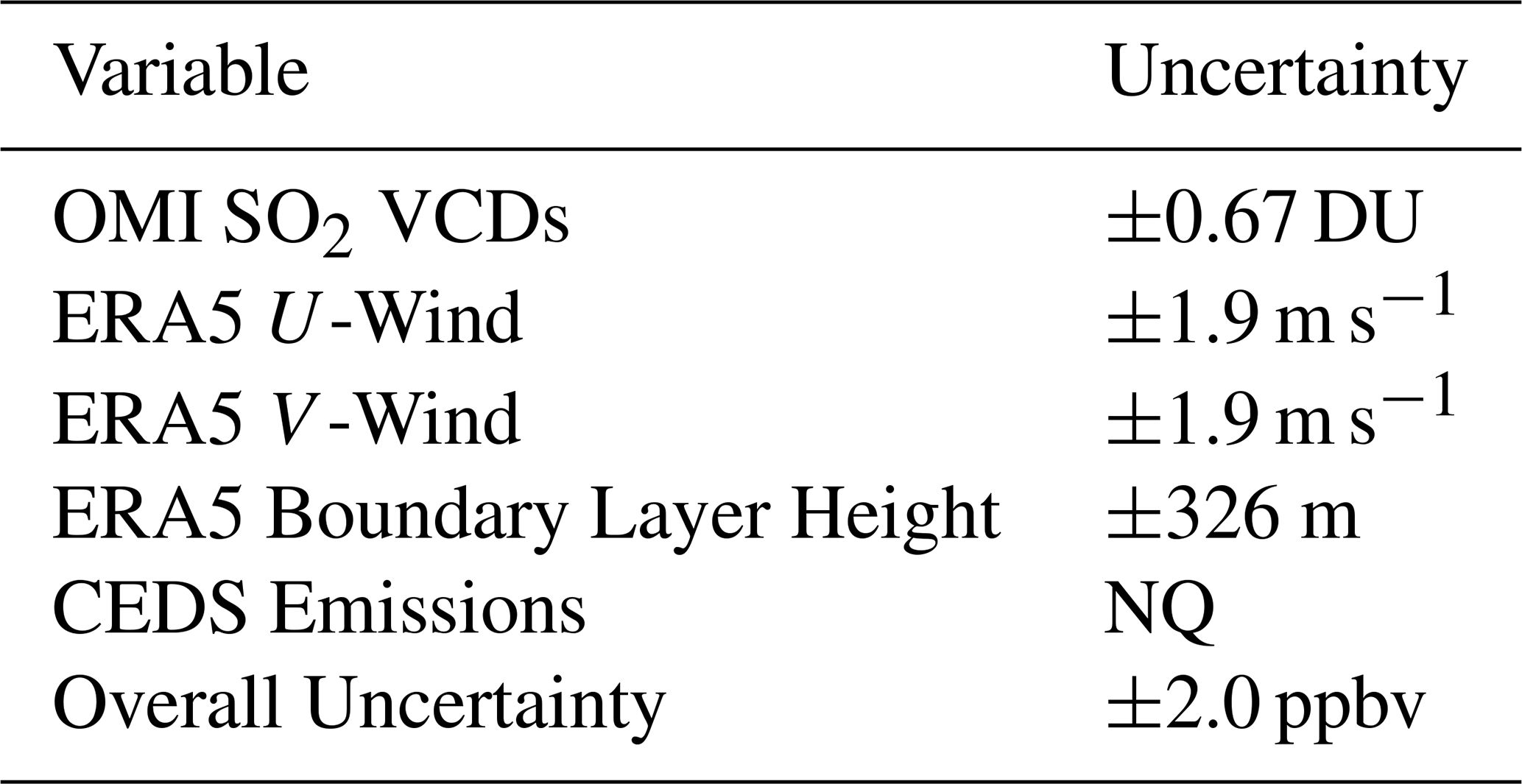
It is much less straightforward to propagate error through a ML model since it effectively acts as a “black box”, so analytical error propagation methods cannot be used. First, uncertainties of the ERA5 meteorological fields were calculated using the moving-block bootstrapping approach. To obtain the overall uncertainty, we used traditional bootstrapping techniques to resample the training dataset with replacement and train an ensemble of XGBoost models to obtain an uncertainty in the model output based on changes in the training data given to the model. To maintain consistency, the same independent testing dataset was used to make the model predictions for each bootstrap. The standard deviation was calculated for each station and day across the different models and was then averaged over space and time to obtain the overall uncertainty. The uncertainties of the ML inputs and overall uncertainty from the retraining analysis are shown in Table 2. For the ML-based method, the overall uncertainty was estimated to be ±2.0 ppbv, which is lower than the propagated error for the CTM-based method. The overall uncertainty for the ML-based method does not directly account for uncertainty in the model inputs, but since traditional error propagation and summation of uncertainties are not possible for ML, this is our best estimate at how the training data can impact the predictions from the model.

Table 2 Sources and magnitudes of uncertainty for the ML-based method. Uncertainties for the OMI SO₂ VCDs and ERA5 meteorology were determined using moving-block bootstrapping. The overall uncertainty for the ML-based method was determined using bootstrapping on the training dataset and retraining multiple XGBoost models to estimate the uncertainty in the model training. The uncertainty for the CEDS inventory was not able to be quantified (NQ).

2.7 Evaluation metrics

To quantify the discrepancies between the estimated surface SO₂ concentrations from the CTM-based method, ML-based method, and the CNEMC in situ measurements, we used several different metrics from previous studies (e.g., Yang et al., 2023b; Zhang et al., 2021, 2022) including the mean absolute error (MAE; Eq. 6), root mean squared error (RMSE; Eq. 7), and relative percent error (RPE; Eq. 8),

$$\begin{array}{}\text{(6)}& {\displaystyle }\mathrm{MAE}={\displaystyle \frac{\mathrm{1}}{N}}\sum _i^N\left|S_{\mathrm{est},i}-S_{\mathrm{CNEMC},i}\right|,\text{(7)}& {\displaystyle }\mathrm{RMSE}=\sqrt{{\displaystyle \frac{\mathrm{1}}{N}}\sum _i^N{\left(S_{\mathrm{est},i}-S_{\mathrm{CNEMC},i}\right)}^{\mathrm{2}}},\text{(8)}& {\displaystyle }\mathrm{RPE}={\displaystyle \frac{\mathrm{1}}{N}}\left(\sum _i^N\left|{\displaystyle \frac{S_{\mathrm{est},i}-S_{\mathrm{CNEMC},i}}{S_{\mathrm{CNEMC},i}}}\right|\right)\times \mathrm{100}\mathit{\%},\end{array}$$

where N is the number of stations, S_est is the estimated surface concentration from the CTM- or ML-based method, and S_CNEMC is the surface concentration from the in situ measurements. Previous studies have also used slopes and correlations from linear regression analyses between the estimated and in situ concentrations to assess the relative magnitudes and spatial distributions, respectively (e.g., Kharol et al., 2017; Lee et al., 2011; McLinden et al., 2014). In Sect. 3.1, results from the CTM-based method were validated and compared to previous studies using the full dataset since they are independent on in situ measurements. In Sect. 3.2, results from the ML-based method were validated and compared to previous studies using only the independent testing dataset. Finally, in Sect. 4, both methods were directly compared using the independent testing dataset (i.e., retained from ML training) such that the comparisons are made on an identical truth dataset for the first time.

3 Estimations of surface SO₂ concentrations from OMI satellite data

3.1 Evaluation of the CTM-based method

Maps, histograms, and scatterplots of the annual mean surface SO₂ concentrations from the CTM-based method and CNEMC in situ measurements are shown in Fig. 3. Both datasets have a similar spatial distribution with the highest concentrations in the North China Plain (Fig. 3), a highly industrialized region with many anthropogenic sources of SO₂ (Fig. 1b). The average correlation between the estimated and in situ concentrations is 0.58, indicating that the CTM-based method can accurately distinguish between polluted and clean areas (Fig. 3). The CTM-based method also captures a 45 % decrease in the concentrations from 2015–2018, also seen in the data from the monitoring network (Fig. 3). Despite the similarities in the spatial distribution and temporal trends, the surface concentrations obtained from the CTM-based method are significantly underestimated. The slope between the estimated and in situ concentrations is 0.24 with an RPE around 75 % (Fig. 3). The discrepancy in the estimated concentrations is also apparent in the frequency distributions with peaks and mean values around 1–3 ppbv compared to around 5–10 ppbv from the in situ measurements. The surface concentrations from the CTM-based method were also separated by season, averaged from 2015–2018, and validated against in situ measurements for the first time. As shown in Fig. S13, the CTM-based method was able to accurately capture the spatial distribution (r = 0.56) and seasonality of the in situ measurements with higher concentrations in the winter and lower concentrations in the summer but still suffered from underestimation (slope = 0.24; RPE = 76 %).

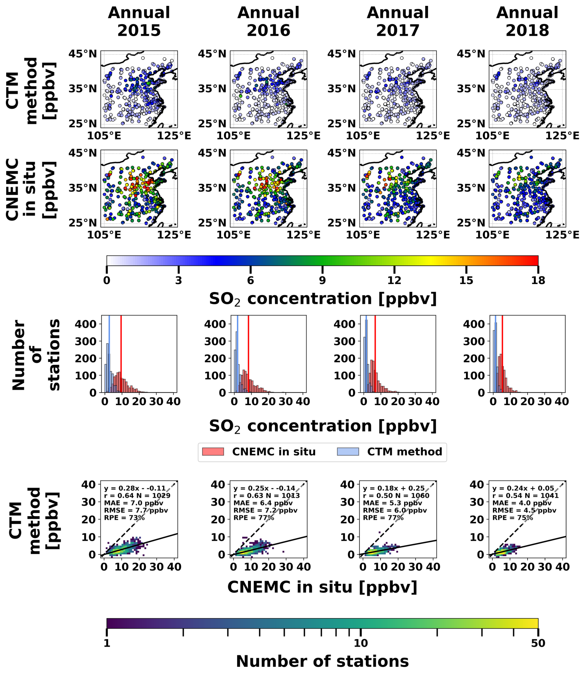
Figure 3 Spatial distributions of the annual average surface SO₂ concentrations from the CTM-based method (top row) and CNEMC in situ measurements (second row), histograms of the surface concentrations from each dataset with vertical bars representing the means (third row), and scatterplots between the two datasets (bottom row). Each column represents a different year in the study period. Histograms and scatterplots are binned every 1 ppbv. Each scatterplot is colored by the number of stations in each bin and includes a linear regression analysis with the best fit line (solid line), best-fit equation, correlation coefficient, total number of stations, 1:1 line (black dashed line), MAE, RMSE, and RPE.

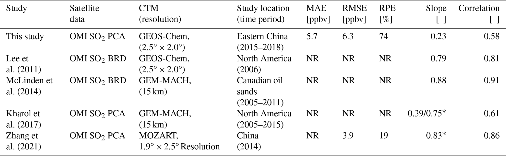
Table 3 summarizes the results from the validation of annual mean concentrations from our study and previous studies using the CTM-based method. The studies by Lee et al. (2011) and McLinden et al. (2014) each utilized the OMI band residual difference (BRD) SO₂ product and used SVRs from coarse- and high-resolution CTMs, respectively. McLinden et al. (2014) outperformed Lee et al. (2011) with slopes of 0.88 and 0.79, respectively, and correlations of 0.91 and 0.81, respectively. Similarly, our study and Kharol et al. (2017) both use the OMI PCA SO₂ product and used SVRs from coarse-resolution and high-resolution CTMs, respectively. Our study had slightly worse performance than Kharol et al. (2017) with slopes of 0.24 and 0.39, respectively, and correlations of 0.58 and 0.61, respectively. These two sets of studies suggest that given the same OMI product, the model resolution may affect the accuracy of the estimated surface concentrations compared to the in situ observations, assuming that the surface monitoring data are accurate. Our sensitivity tests comparing the impact of spatial resolution on the accuracy of the CTM-based method (Fig. S5) showed a discrepancy in the correlations of 0.05 between GEOS-Chem and GEOS-CF compared to a difference of 0.03 between our study and Kharol et al. (2017); however, the sensitivity tests only showed a discrepancy in the slopes of 0.02 between GEOS-Chem and GEOS-CF, which is much smaller than the 0.15 difference in slopes between our study and Kharol et al. (2017). This suggests that the difference in spatial resolution of our CTM simulations may account for the discrepancy in the correlations between our study and Kharol et al. (2017), but not the slopes, indicating that there may be another factor contributing to the underestimation of the CTM-based method. Additionally, previous studies have also shown that there are differences in SO₂ VCDs across different retrieval algorithms and sensors (Wang and Wang, 2020). The higher slopes from the BRD product may be due to a high bias in the retrievals in polluted areas whereas the PCA product is thought to be more accurate (Li et al., 2013). Additionally, the slope of 0.75 from Kharol et al. (2017) and the results from Zhang et al. (2021) use a scaling factor on the in situ measurements to eliminate some of the bias, so these results are not directly comparable to our study.

Table 3 Comparison of study design (satellite data, model name and resolution, study location and study period) and performance metrics (mean absolute error, root mean square error, relative percent error, slope, and correlation) between our study and previous studies that utilized the CTM-based method for annual mean surface SO₂ concentrations. NR indicates that the value was not reported, and asterisks (^*) indicate a scaling factor applied to the in situ surface concentrations.

Inaccuracies in the CTM-based method can be partially attributed to noise in the satellite data. Individual VCD retrievals have large uncertainties estimated from 60 %–120 % from Li et al. (2020a) and 136 % from our bootstrapping analysis (Table 1), making it difficult to compare to the ground-based measurements on short timescales; however, the noise in the data can decrease with temporal averaging by a factor of $n^{\mathrm{1}/\mathrm{2}}$ where n is the number of measurements being averaged (Krotkov et al., 2008). As a result, longer averaging periods (i.e., annual means) tend to have better performance than shorter timescales (i.e., seasonal means). Additionally, the consistent underestimation of the CTM-based method may be a result of either underestimated SVRs from the GEOS-Chem simulations or a low bias in the OMI PCA product. Figure S6 suggests that the SVRs from GEOS-Chem are typically between 70 %–90 % lower than observed SVRs calculated from CNEMC in situ surface concentrations and OMI VCDs, which is similar to the discrepancy in the surface concentrations from the CTM-based method compared with the in situ measurements. Based on the error propagation from Sect. 2.6, the combined methodological uncertainty of the CTM-based method considering both the OMI retrievals and GEOS-Chem SVRs is ±4.9 ppbv (Table 1). This is larger than most of the estimated surface concentrations shown in the histograms from Fig. 3, indicating the methodological uncertainty associated with this method is large and is highly affected by the accuracy of the input data.

3.2 Evaluation of the ML-based method

The spatial distribution, frequency distribution, and validation scatterplots of the ML and CNEMC annual mean surface SO₂ concentrations from the independent testing dataset are shown in Fig. 4. The ML model estimated the surface concentrations more accurately than the CTM-based method with an improved average correlation of 0.77, lower RPE of 33 %, and an average slope of 0.69. These improvements indicate that the ML-based method has better accuracy in the spatial distributions and magnitudes compared to the CTM-based method. The ML estimated concentrations also have a 45 % decline from 2015–2018, which is the same as the CNEMC in situ measurements (Fig. 4). The shapes of the ML-based frequency distributions also agree well with the CNEMC observations with peaks at the same concentrations (5–10 ppbv) and similar ranges (Fig. 4). The ML-derived and in situ concentrations were also assessed using the seasonal concentrations averaged from 2015–2018. As shown in Fig. S14, the ML-based method was able to capture the spatial distribution (r = 0.72), seasonality, and magnitudes (slope = 0.64; RPE = 36 %) of the seasonal mean surface concentrations more accurately than the CTM-based method. Additionally, the overall uncertainty of the ML-based method is much lower than the CTM-based method at around ±2 ppbv (Table 2). Since the ML predictions have a much larger magnitude, the methodological uncertainty for the ML-based method appears to be more reasonable compared to the CTM-based method.

Figure 4 Spatial distributions of the annual average surface SO₂ concentrations from the ML-based method (top row) and CNEMC in situ measurements (second row), histograms of the surface concentrations from each dataset with vertical bars representing the means (third row), and scatterplots between the two datasets (bottom row). Each column represents a different year in the study period. Histograms and scatterplots are binned every 1 ppbv. Each scatterplot is colored by the number of stations in each bin and includes a linear regression analysis with the best fit line (solid line), best-fit equation, correlation coefficient, total number of stations, 1:1 line (black dashed line), MAE, RMSE, and RPE.

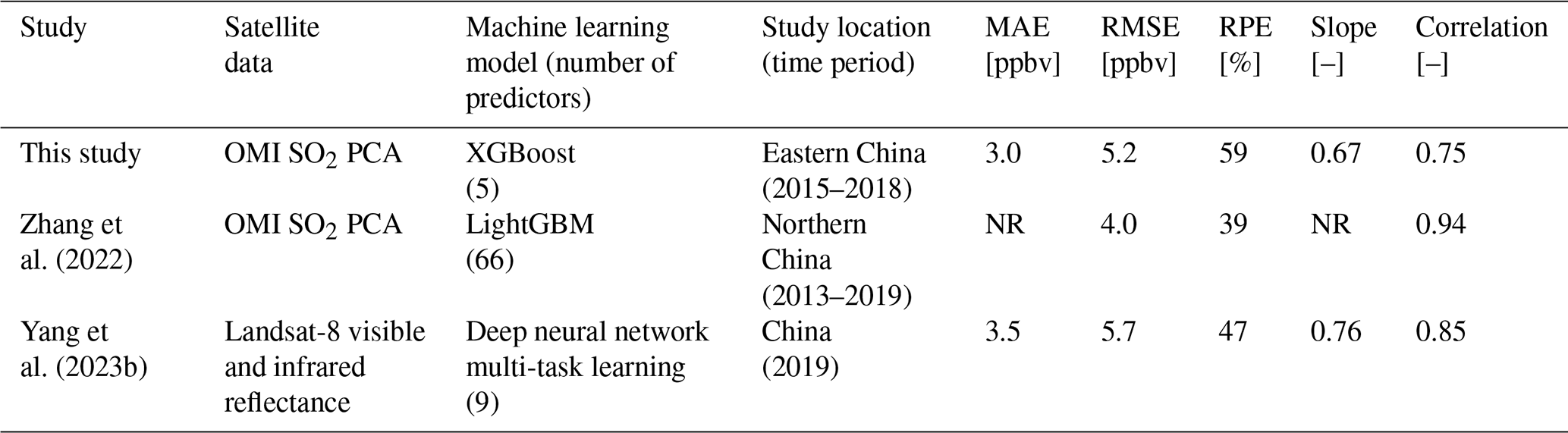
Previous studies have shown that ML models can skillfully capture day-to-day variations in surface SO₂ concentrations in addition to the annual and seasonal means as summarized in Table 4 (e.g., Zhang et al., 2022; Yang et al., 2023b). The estimated daily surface concentrations from our independent testing dataset had a slope of 0.67, correlation of 0.76, and RPE of 58 % compared to the in situ measurements, indicating good performance on short timescales (Fig. 2; Table 4). The performance of our model was comparable to previous studies but had a slightly larger discrepancy (Table 4). Our ML model only used five predictors compared to nine in Yang et al. (2023b) and 66 in Zhang et al. (2022), which may partially account for the increased discrepancy. Additionally, our study did not use any spatial or temporal proxies, which could also explain the slight reduction in performance compared to other studies that have used them.

Table 4 Comparison of study design (satellite data, machine learning model type and number of predictors, study location and study period) and performance metrics (mean absolute error, root mean square error, relative percent error, slope, and correlation) between our study and previous studies that utilized a ML-based method for daily surface SO₂ concentrations. NR indicates that the value was not reported.

We performed a permutation importance analysis to assess how each predictor impacted the model predictions. Figure 5a indicates that the boundary layer heights and OMI SO₂ VCDs are the two most influential predictors followed by emissions and wind speeds. It is also worth noting that all of the predictors contribute toward the estimated surface concentrations with all permutation importance scores falling between 0.2 and 0.5 with none being unused. The boundary layer heights have a much smaller variation on short timescales compared to the OMI SO₂ VCDs. Based on the bootstrapped uncertainties from Table 2, the relative standard deviations are 20 % for boundary layer heights, and 136 % for OMI VCDs. As a result, the ML model is likely able to learn the relationship between boundary layer height and surface SO₂ concentrations more easily than the OMI SO₂ VCDs. Scatterplots between each ML predictor variable and the ML estimated surface SO₂ concentrations with Spearman rank coefficients (r_s) are shown in Fig. 5b–f. The ML-derived SO₂ concentrations increase with larger SO₂ VCDs and emissions, as well as decrease with increasing boundary layer heights and wind speeds (Fig. 5b–f). The surface concentrations and boundary layer heights each have a strong, inverse seasonality, as shown in Figs. S14 and S15, respectively, so the strong temporal correlations between them also likely lead to a high permutation importance in the model. The behavior of the ML predictions is consistent with the expected physical relationships between each predictor and the surface SO₂ concentrations. Large OMI VCDs and emissions indicate areas of high SO₂ loading, and large boundary layer heights and wind speeds lead to mixing and the dilution of SO₂. The magnitudes of the r_s values are small, indicating that the model may be making predictions based on the interactions between variables rather than any individual predictor. The small number of predictors used in our model allows us to link the ML predictions to known atmospheric processes, adding confidence to the model in its ability to accurately estimate the surface concentrations.

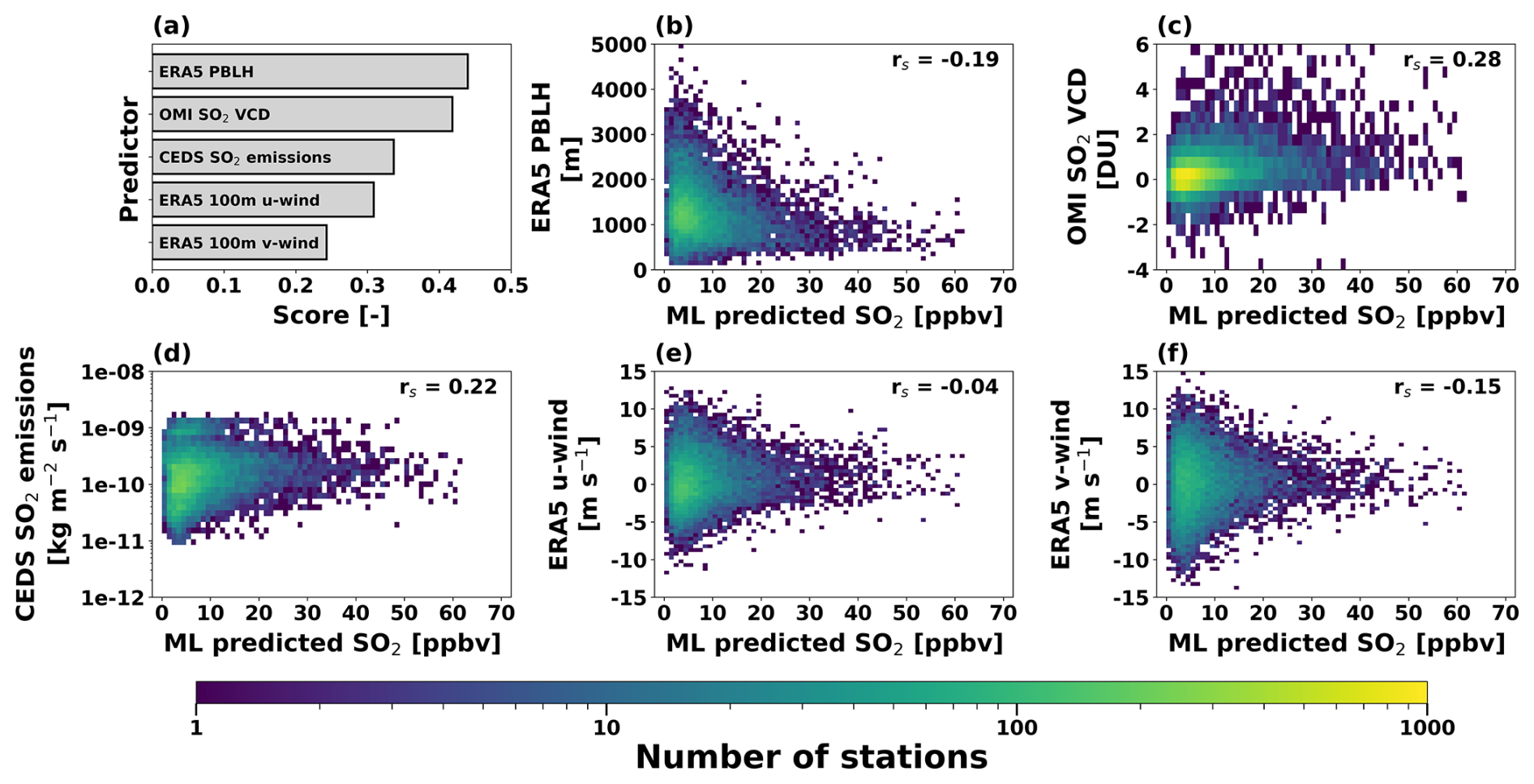
Figure 5 Evaluation of the daily ML-predicted surface concentrations using (a) permutation importance analysis, and scatterplots showing the ML predictor variables against the ML estimated surface SO₂ concentrations for (b) ERA5 PBLH, (c) OMI SO₂ VCDs, (d) CEDS SO₂ emissions, (e) ERA5 U-wind speeds, and (f) ERA5 V-wind speeds. Each scatterplot is colored by the number of stations in each bin and includes the Spearman rank coefficient (r_s).

4 Direct comparison of the CTM- and ML-based methods

The validation results from the CTM-based method in Sect. 3.1 were based on the full dataset since the estimated surface concentrations are independent of the in situ monitoring data; however, the validation results from the ML-based method in Sect. 3.2 were only based on 10 % of the data that was and reserved for an independent validation and not used for training. The comparison of these results using different datasets is still important but does not provide a direct comparison of their performance. Here, the CTM- and ML-based methods were directly compared using the same truth dataset over the same locations and study period for the first time. Each method was resampled to match the independent testing dataset (i.e., data retained from ML training) and the performance of each method was assessed given identically sampled data. First, each technique was validated at the CNEMC measurement sites in Sect. 4.1, similar to the analyses in Sect. 3. Then, both methods will be used to create gridded surface SO₂ concentrations in Sect. 4.2 to assess how effective both methods are for filling in the gaps of the CNEMC monitoring network, one of the main motivations for estimating surface concentrations from satellite VCDs.

4.1 Performance on independent data

Scatterplots between the in situ concentrations and estimates of the surface concentrations from both the CTM- and ML-based methods for the testing dataset are shown in Fig. 6. The surface concentrations estimated by the ML model are much closer to the in situ measurements (i.e., the 1:1 line) than the CTM-based method, which is consistent with the previous results in Figs. 3–4. For the annual mean concentrations, the ML-based method had an average slope of 0.69 and correlation of 0.77, compared to values of 0.18 and 0.30, respectively, from the CTM-based method (Fig. 6a–d). The ML model also outperforms the CTM-based method on the seasonal data averaged over 2015–2018. The ML-based method had an average slope and correlation of 0.64 and 0.73, compared to 0.19 and 0.31, respectively, from the CTM-based method (Fig. 6e–h). The CTM-based method performed worse on this smaller dataset compared to the full dataset in Sect. 3.1 due to less temporal averaging, leading to larger discrepancies with the in situ measurements. There is a smaller decrease in the performance of the ML-based method compared to the CTM-based method when assessing the performance of individual seasons rather than the 2015–2018 average for each season, as shown by Fig. S16. The slope and correlation for the ML-based method each decreased by around 0.1 to 0.59 and 0.67, compared to a decrease of 0.05 and 0.1 to 0.15 and 0.22, respectively, for the CTM-based method (Fig. S16). On both annual and seasonal timescales, the ML-based method more accurately captured the spatial distribution and magnitudes of the surface SO₂ concentrations compared to the CTM-based method.

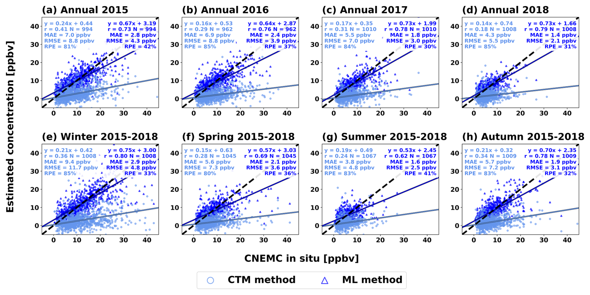
Figure 6 Scatterplots showing the estimated surface SO₂ concentrations from the CTM-based method (light blue squares) and ML-based method (dark blue triangles) against the in situ measurements from the independent dataset for (a–d) annual mean concentrations for each year in the study period, and (e–h) the 2015–2018 mean concentrations separated by season. Each scatterplot includes a linear regression analysis with the best fit line (solid lines), best-fit equation, correlation coefficient, total number of stations, 1:1 line (black dashed line), MAE, RMSE, and RPE.

Time series of the annual and seasonal mean surface SO₂ concentrations from the in situ measurements, and estimated concentrations from the CTM- and ML-based methods are shown in Fig. 7a–b. The ML estimated concentrations were much closer to the CNEMC measurements than the CTM-based method. The mean ML concentrations had an average discrepancy of 5 % with the in situ measurements, compared to a discrepancy of 58 % from the CTM-based method (Fig. 7a–b). The ML-based method also captured the same temporal variations as the in situ measurements each with a 44 % decrease in concentrations from 2015–2018, and an average seasonal fluctuation by a factor of 1.9 between the winter and summer seasons (Fig. 7a–b). The CTM-based method also had good agreement in the temporal trends of the in situ measurements but was not as good as the ML-based method with a 36 % decrease from 2015-2018 and a seasonal fluctuation by a factor of 2.4 (Fig. 7a–b). Since the CTM-based surface SO₂ concentrations were underestimated, the magnitude of the temporal trends is much smaller than the observations and ML-based method, but the relative change was similar, as shown by Table S1 in the Supplement. The decrease in SO₂ from 2015–2018 detected by both methods is consistent with previous studies that showed a reduction in emissions over China shown using satellite VCDs (Li et al., 2017; Wang and Wang, 2020), satellite-derived emissions (Fioletov et al., 2023), and surface concentrations (Wei et al., 2023; Zhang et al., 2021). Despite the similarities in the year-to-year and season-to-season variations, the greatest difference between the time series of the two methods was the magnitude of the concentrations.

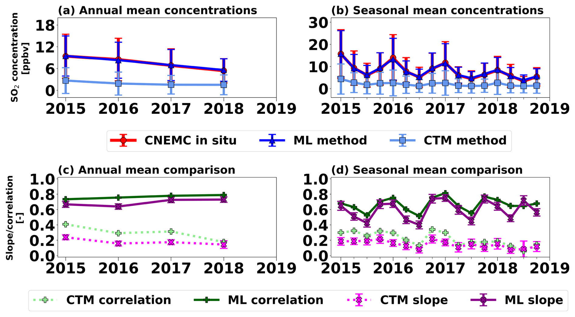
Figure 7 Time series of the surface SO₂ concentrations from the CTM-based method (light blue squares), ML-based method (dark blue triangles), and CNEMC in situ measurements (red circles) from the independent dataset as (a) annual and (b) seasonal means, as well as the slopes (pink x's) and correlations (green crosses) from the (c) annual and (d) seasonal mean validations between the CTM-based method (dashed line) and ML-based method (solid line) with the in situ measurements. Error bars on the concentrations represent a 1 standard deviation uncertainty, and error bars on the slopes represent a 95 % confidence interval based on the standard error of the linear regression fit. Data for all panels can be found in Table S1.

To assess how the accuracy of each method changed over time, time series of the slopes and correlations from the annual and seasonal comparisons between the estimated and in situ surface concentrations from Fig. S16 and Table S1 are shown in Fig. 7c–d. For the entire study period, the performance of the ML-based method was more accurate than the CTM-based method as indicated by the higher slopes and correlations (Fig. 7c–d). Additionally, the CTM-based method suffered from a decrease in accuracy over time alongside declining SO₂ concentrations while the ML-based method remained stable from year to year (Fig. 7c–d). The accuracy of the CTM-based method is highly dependent on noise in the satellite data. As SO₂ loading decreased over China, it became more difficult for OMI to detect, which may have introduced additional noise into the VCDs. Comparatively, the ML-based method was more resistant to noise in the satellite data. As SO₂ VCDs decreased, the ML predictions can utilize other predictors such as meteorology and emissions to estimate the surface concentrations, limiting the impact of the noisy satellite data (Fig. S17a–d). The accuracy of the ML-based method also had a distinct seasonality with generally better performance in the winter and worse in the summer (Fig. 7d). The boundary layer heights and OMI SO₂ VCDs were the dominant predictors in the winter, whereas the CEDS emissions and boundary layer heights were the dominant predictors in the summer (Fig. S17e–h). The CEDS emissions are less consistent with the in situ measurements than the OMI VCDs with r_s values of 0.22 and 0.28, respectively (Fig. 5), which may account for the increased discrepancy of the ML-derived concentrations during the summer.

In summary, both the CTM- and ML-based methods captured similar temporal variations as the in situ measurements, but the ML-based method was more accurate and had more stable performance over time compared to the CTM-based method, which had decreasing performance over time, likely due to increased noise in the satellite data from decreasing SO₂ loading.

4.2 Comparison of gridded products

The CTM- and ML-based methods were used to create gridded surface SO₂ concentrations at 0.25° × 0.25° horizontal resolution to assess how effective each technique is for filling in the gaps of the CNEMC air quality monitoring network. The gridded annual mean surface SO₂ concentrations from the CTM- and ML-based methods are shown in Fig. 8. Both methods produced similar spatial distributions to one another over land with the highest concentrations in the North China Plain and lower concentrations elsewhere. Over land, each method also has a spatial distribution similar to the retrieved SO₂ VCDs from OMI as shown in Fig. S18a–d, further indicating that both methods effectively utilizing the OMI data. Over the oceans, there is disagreement in the spatial distributions with the ML-based method producing high concentrations and the CTM-based method producing low concentrations. Since the ML predictions are significantly affected by boundary layer heights (Fig. 5), the model is likely incorrectly associating the low marine boundary layer with areas elevated SO₂, as suggested by the seasonally averaged ERA5 boundary layer heights in Fig. S15. Inaccuracies over the oceans have also been reported in Kang et al. (2021) where ML was used to estimate surface concentrations of NO₂ and ozone and was attributed to a lack of training data for the ML model in these locations. Since the ML model was only trained for conditions over land, it learned the relationship between high surface SO₂ concentrations and low continental boundary layer heights during the winter months but could not accurately apply this knowledge over the oceans. As a result, the CTM-based method may produce more reasonable spatial distributions of surface SO₂ concentrations in locations with a lack of surface observations where a ML model cannot be trained.

As shown in Fig. 8, both gridded products captured the decrease in annual mean concentrations from 2015 to 2018 observed at the CNEMC sites. Both methods were also able to capture the seasonal variations in their gridded products with the highest concentrations in the winter and lowest concentrations in the summer, as shown in Fig. S19. The seasonal gridded surface SO₂ concentrations were also still consistent with the OMI SO₂ VCDs (Fig. S18e–h). Although it is not possible to validate the gridded products, since the ML-based method had more accurate spatial distributions, temporal variations, and magnitudes than the CTM-based method when validated at the CNEMC sites, the gridded product is likely to be more accurate as well, but only over land. The unexpected area of elevated concentrations over the oceans exposed a major limitation of the ML-based method and suggests that future work in improving the CTM-based method may be worthwhile, especially for estimating surface SO₂ concentrations in locations where training data are not available.

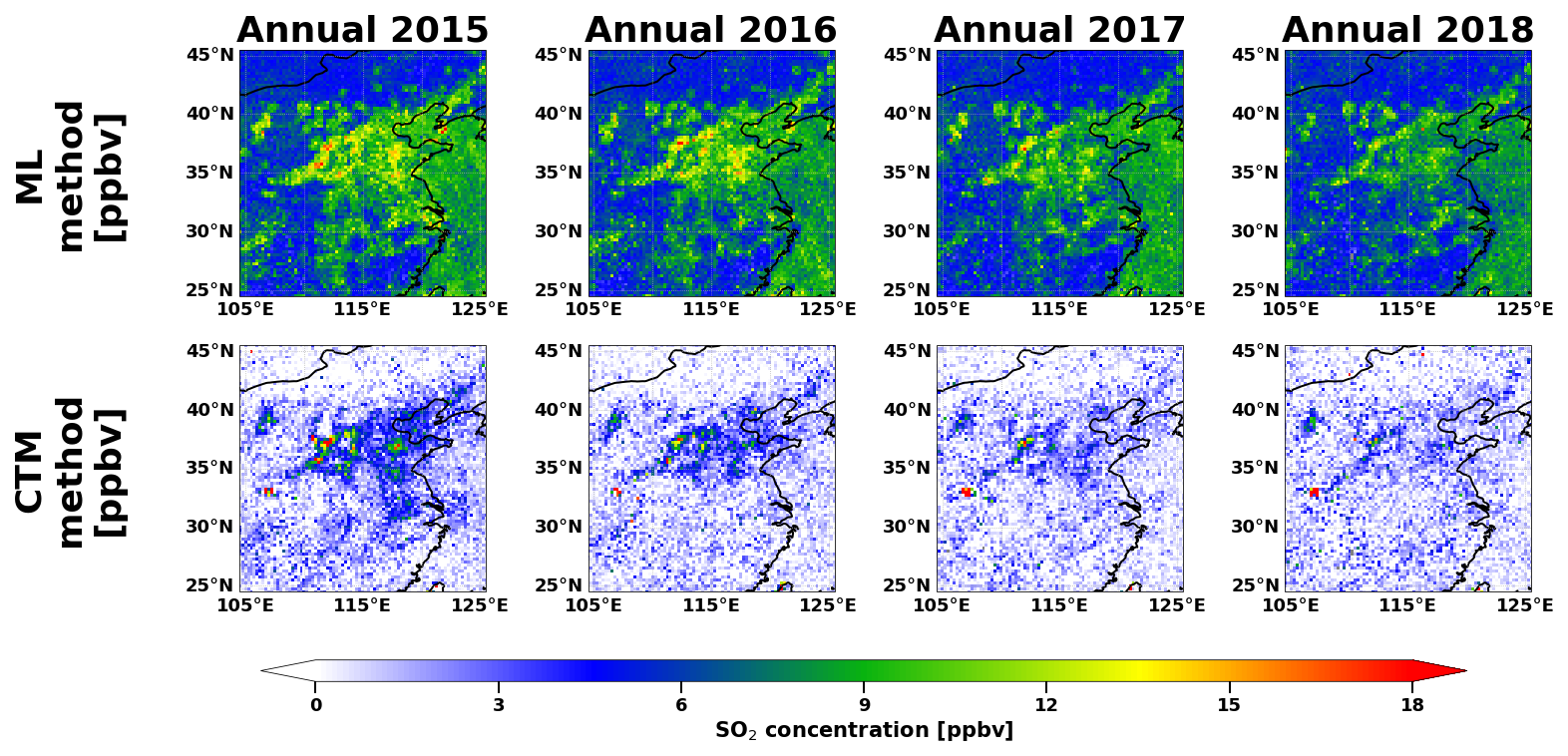
Figure 8 Maps of the annual mean surface SO₂ concentrations in ppbv from the ML-based method (top row) and CTM-based method (bottom row) over the study area at 0.25° × 0.25° horizontal resolution. Each column represents a different year of the study period.

5 Discussion and Conclusion

In this study, we estimated surface SO₂ concentrations over eastern China from 2015–2018 using OMI SO₂ VCDs with two different methodologies. First, we used simulated SVRs from the GEOS-Chem model to convert the OMI SO₂ VCDs into surface concentrations using the CTM-based method. Then, we used an XGBoost model to statistically relate OMI VCDs, ERA5 meteorology, and CEDS SO₂ emissions to in situ surface concentrations using the ML-based method. The novelty of this study includes a first time investigation of quantifying methodological uncertainties for both the CTM- and ML-based techniques, a validation of seasonal mean surface concentrations from the CTM-based method, and a direct comparison between the two methods on the same truth dataset.

We found that the ML-based method was more accurate than the CTM-based method at estimating the surface concentrations when validated against in situ measurements from the CNEMC air quality monitoring network. The ML-based method had a discrepancy of ∼ 30 % with no significant bias (slope = 0.69), whereas the CTM-based method had a discrepancy of ∼ 75 % with a significant underestimation (slope = 0.24). Despite the underestimation, the CTM-based method also produced surface SO₂ concentrations that had similar spatial distributions (r = 0.58) and temporal patterns as the CNEMC in situ measurements, similar to previous studies. The CTM-based method requires averaging data over relatively long timescales to reduce the noise in the satellite retrievals and obtain more accurate estimates of the surface concentrations. The underestimation of this method is likely due to a low bias in the simulated SVRs. The CTM-based method also suffered from decreasing accuracy over time due to decreasing SO₂ loading over time since the retrieval that has a low signal-to-noise ratio. In addition to lower discrepancies, the ML-based method outperformed the CTM-based method in terms of the spatial distribution (r = 0.77) and temporal variations. The accuracy of the ML-based method was especially apparent for smaller datasets that have limited temporal averaging and noisier OMI data since the model can rely on other predictors, which was indicated by the stable accuracy over time. Even though our ML model was only based on five input variables, the results were similar to previous studies that used far more predictors. The small number of predictors also allowed us to relate the model predictions and input variables to known physical processes such as pollutant emissions and dispersion, thus lending more confidence in our ML model as compared with other “black box” ML models. Finally, both methods were used to create gridded products to provide estimates of surface SO₂ concentrations in locations that do not have access to ground-based air quality monitoring measurements. This analysis exposed a major limitation in the ML-based method where it produced unrealistic spatial distributions of SO₂ over the ocean since it was only trained on data from over the land. Despite the underestimation of the CTM-based method, there is still value in using it to estimate surface SO₂ concentrations in locations where there is no training data available for developing ML-based techniques, but additional steps should be taken to decrease the underestimation of this method.

In addition to using these estimated surface concentrations for filling in the gaps of air quality monitoring networks, the gridded products can be used to investigate other chemical processes in the atmosphere related to SO₂, such as estimating sulfuric acid concentrations and parameterizing aerosol nucleation and growth. New particle formation studies in China have shown that strong and frequent aerosol nucleation events occur in the presence of SO₂ in both heavily polluted urban (Dai et al., 2017; Wu et al., 2007) and relatively cleaner rural locations (Dai et al., 2017; Du et al., 2022). Estimating surface SO₂ concentrations using these satellite-based methods may be helpful for predicting the locations and intensities of new particle formation events or estimating sulfuric acid concentrations, especially for locations without in situ measurements or air quality monitoring sites.

In the future, the performance of these methods may be improved by higher-resolution satellite data, which may help to improve the results. OMI can only detect sources as small as 30 kt yr⁻¹, but newer instruments like the Tropospheric Monitoring Instrument (TROPOMI; Veefkind et al., 2012) or can detect sources as small as 8 kt yr⁻¹ (Fioletov et al., 2023). Additionally, geostationary satellites like Tropospheric Emissions: Monitoring of Pollution (TEMPO; Zoogman et al., 2017) may offer future opportunities to estimate surface concentrations of air pollutants at even higher spatial and temporal resolution, which may improve the accuracy of both methods. Additionally, this study only focused on SO₂, but both methods can also be applied to other air pollutants such as NO₂, ozone, and particulate matter to see if the relative performance of each method is similar for other species. Since these two methods can utilize space-based measurements to fill in the gaps of ground-based air quality networks, investigating their relative performance as improvements are made to the satellite retrievals, CTMs, and ML models is critical for monitoring near-surface air pollution with high accuracy in locations where traditional observations are not possible.