Evaluating urban methane emissions and their attributes in a megacity, Osaka, Japan, via mobile and eddy covariance measurements

Urban areas are regions where large greenhouse gas emissions are expected, but in many urban areas, the sources and sinks remain uncertain. In this study, we conducted mobile and eddy covariance measurements to evaluate CH₄ emissions in the megacity Osaka, Japan. Based on the mobile measurements, several elevated CH₄ concentrations were observed. Most locations were not related to CH₄ sources identified by emission inventories reported by local governments. Two platforms for mobile measurements, vehicle and bicycle, showed good consistency for estimating total CH₄ emissions, but vehicle measurements tended to yield smaller natural gas emission estimates than bicycle measurements. CH₄ emissions from bicycle measurements were adjusted using daytime CH₄ fluxes via the eddy covariance method for flux footprint areas and used to upscale to Sakai and Osaka cities. Using these upscaled emissions from vehicle measurements as a proxy for total area fluxes the estimated CH₄ emissions were 10 021 ± 1000 t CH₄ yr⁻¹ for Osaka and 2379 ± 480 t CH₄ yr⁻¹ for Sakai, 18 times and 2.5 times greater, respectively, than inventory estimates. Coincident C₂H₆ observations indicated that natural gas emissions contributed 64 % of the total CH₄ emissions in Osaka city and 47 % in Sakai city. From these snapshots, the CH₄ emissions from the metropolitan areas in Japan may be considerably greater than the emission inventories, and most CH₄ sources are not well characterized in those inventories. These unaccounted sources need to be better characterized to improve the Japanese CH₄ inventory and assess whether these emissions can be mitigated.

1 Introduction

Cities are among the major sources of greenhouse gases and are thus important targets for emission reduction (e.g., Crippa et al., 2021). In particular, methane (CH₄) emission reduction is important in the medium term because CH₄ is a powerful greenhouse gas whose global warming potential is 84 times greater than that of carbon dioxide (CO₂) for a 20-year time horizon. Consequently, there is an urgent need to reduce CH₄ emissions for a short-term positive effect on climate warming. Recent measurements of CH₄ concentrations and fluxes in urban areas suggest that substantial CH₄ emissions occur in many cities and that emission inventories are highly uncertain, especially in terms of urban natural gas emissions (Helfter et al., 2016; Sargent et al., 2021). More independent assessments of emission inventories for different cities are needed to drive effective mitigation actions.

In recent years, measurements using vehicle-mounted instruments have been carried out in urban areas to compare CH₄ emissions among different urban environments. These studies highlighted that (1) urban regions are significant CH₄ sources (Vogel et al., 2024); (2) some CH₄ sources do not account for the current inventories (Vogel et al., 2024); (3) non-negligible levels of gas leak from sewer networks (Fernandez et al., 2022; Joo et al., 2024) or underground gas pipelines, mostly old corrosion-prone pipelines (Defratyka et al., 2021; von Fischer et al., 2017); and (4) a small number of high CH₄ emission rates mostly account for an area's total CH₄ emissions (Maazallahi et al., 2020). Previous studies have also revealed large varieties of emission characteristics in terms of emission intensity and attributions. Currently, most of these measurements have been conducted in Europe and North America (e.g., Vogel et al., 2024), and most Asian megacities, except Seoul, South Korea (Joo et al., 2024), are underrepresented.

Ethane (C₂H₆) is a useful tracer for estimating leakage from natural gas distribution systems, as natural gas has a characteristic CH₄ to C₂H₆ ratio. Gas leakage was recently estimated on the basis of simultaneous measurements of CH₄ and C₂H₆ concentrations (Jackson et al., 2014; Fernandez et al., 2022). In Japan, the major gas companies in Tokyo and Osaka have stated that they supply natural gas with representative compositions of 89.6 % CH₄ and 5.6 % C₂H₆ (Tokyo) and 88.9 % CH₄ and 6.8 % C₂H₆ (Osaka). This suggests that natural gas leakage would simultaneously increase gas concentrations with a ratio of atmospheric concentration (ΔC₂H₆ $/$ ΔCH₄) of approximately 0.07 during downwind enhancement. Direct measurements of CH₄ and C₂H₆ fluxes should provide further information on the contributions of natural gas leakage in urban areas.

Eddy covariance (EC) methods are powerful tools for measuring spatially representative fluxes of greenhouse gases (Baldocchi, 2014). The EC method directly measures fluxes of trace gases between the land surface and atmosphere from the footprint upwind of the measurement point. The EC measurement represents a spatially integrated flux, where the flux footprint depends on the wind direction, height of the measurement, and atmospheric stability. The EC method has been used for measuring fluxes over terrestrial ecosystems (Baldocchi, 2014) and has been applied in urban areas to understand decade-long greenhouse gas emissions (Helfter et al., 2016; Liu et al., 2020; Ueyama and Takano, 2022). For urban areas, EC measurements have shown diurnal, seasonal and spatial variabilities in CO₂ fluxes in various cities (Helfter et al., 2016; Nordbo et al., 2012; Ueyama and Ando, 2016). Recently, CH₄ emissions have also been measured via the EC method in various cities (Gioli et al., 2013; Helfter et al., 2016; Pawlak and Fortuniak, 2016; Stichaner et al., 2024), which has demonstrated that urban areas are important CH₄ sources that are not fully characterized by the current inventories. Although the EC method provides spatially integrated fluxes, identifying detailed emission characteristics, such as the locations of emission hotspots and source attributes (natural gas or biogenic sources), is difficult. Simultaneous EC and mobile measurements may provide additional insight into urban CH₄ emissions (Takano and Ueyama, 2021).

On the basis of a governmental inventory (NGGIDJ, 2024), CH₄ emissions from Japan decreased from 1.74 × 10³ t CH₄ yr⁻¹ in 1990 to 1.07 × 10³ t CH₄ yr⁻¹ in 2022. The contributions of CH₄ emissions to total greenhouse gas emissions are small (2.6 % in 2022). Among the country-scale CH₄ emissions in 2022, the agricultural sector accounts for the most important CH₄ emission (81.9 % of the total emission), and the waste sector (e.g., landfills, sewage treatment plants) accounts for 12.1 % of the emission. The leakage of natural gas is considered to be a minor CH₄ source (0.8 %) in Japan. Although sophisticated emission datasets (Ito et al., 2019; NGGIDJ, 2024) have been developed, and intensive field campaigns for rice paddies have been conducted (Itoh et al., 2011), urban CH₄ emissions have not been evaluated with atmospheric measurements in Japan.

In this study, we conducted mobile measurements of CH₄ and C₂H₆ concentrations and EC measurements of CH₄ fluxes to evaluate urban CH₄ emissions and their attributes in the metropolitan area of Osaka. Osaka is the second largest megacity in Japan and is therefore a priority target for characterizing urban CH₄ emissions. Our specific objectives are as follows.

1. Based on vehicle-based mobile measurements covering various urban areas from the city center to rural areas in Osaka Prefecture, can we understand emission characteristics on the basis of urban intensity?

2. Does the vehicle-mounted survey capture a true snapshot of an area's emission profile? We examine additional bicycle measurements that cover all streets within a target area for comparison.

3. Can regional-scale CH₄ emissions beyond the EC footprint be estimated by using mobile measurements scaled to EC-derived fluxes?

4. How does Osaka compare with other major international cities in terms of urban methane emissions abatement potential?

2 Method

2.1 Target area

The study area is the metropolitan area in Osaka, which is the second largest metropolitan area in Japan and includes two government-decreed cities: Osaka and Sakai. The population densities of Osaka and Sakai are 12 325 and 5514 km⁻², respectively. The areas are highly urbanized. The total lengths of the roads within Osaka and Sakai are 3712 and 2122 km, respectively. For natural gas distributions by a local gas company, the pipeline material for low-pressure gas is mostly polyethylene (PE), whose penetration is 89 %. Other less prevalent materials include gray cast iron pipes, polyethylene-lined steel pipes and galvanized steel pipes (https://www.daigasgroup.com/sustainability/, last access: 10 December 2024). Approximately 96 % of Osaka city sewer pipes use combined sewer systems, where both wastewater and stormwater flow through the same pipes. In Sakai city, only the northwest area (mostly Sakai Ward), which accounts for 12 % of the city area, uses combined sewer systems.

2.2 Mobile measurements

We conducted two types of mobile measurements: vehicle and bicycle platforms. The vehicle measurements were intended to understand the characteristics of CH₄ emissions within Osaka Prefecture. The vehicle measurements were conducted along a gradient of urbanization from a dense city center in Osaka city, such as major commercial, business, and shopping districts (Umeda, Namba, and Tennoji), to rural areas in southern Sakai city. The bicycle measurements were conducted to cover all roads, including narrow streets that could not be driven by a vehicle, within the target area to ensure that almost no omissions occurred in the vehicle measurements and to clarify the overall picture of the emission sources within the area. The bicycle measurements were conducted mostly in Sakai, Kita, and Naka wards of Sakai city.

We conducted mobile measurements using a vehicle, mostly covering Osaka and Sakai cities (Fig. A1; Table A1). For each city, intensive mobile measurements were performed during the daytime on weekdays (25–29 September, 13–17 November 2023 for Sakai; 9–13 October, 11–15 December 2023 for Osaka; 18–22 November 2024 for Osaka). Additional mobile measurements using a vehicle were performed for coastal areas containing potential CH₄ hotspots, such as sewage treatment plants and a landfill in Osaka Prefecture. Prior to the vehicle measurements, we set a target area each day, and the vehicle drove evenly on major roads and small streets within the target areas where the vehicle could pass. In addition to this strategy, we also visited areas near known emission sources, such as sewage treatment plants and dairy farms. To measure air near point sources, we conducted our observations in orbit around a potential point source if roads were publicly open; otherwise, we drove the roads closest to the source. Repeated observations were not conducted to prioritize observations of large areas, but several repeated observations were conducted for the dairy farm and the sewage treatment plants in Sakai city. The total distance driven by the vehicle during the collection of measurements was 2558 km: 1280 km for Osaka city, 1049 km for Sakai city, and 167 km for other cities. The mean vehicle speed each day was 17.0 ± 7.5 km h⁻¹.

The vehicle measurements provided the CH₄, C₂H₆, and water vapor concentrations via a laser-based analyzer (MIRA Ultra, Aries Technologies, USA), the wind speed and direction via a sonic anemometer (Portable Mini, Calypso Instruments, USA), and the location via a global positioning system (GPS) (16X-HVS, Garmin, USA). These instruments were installed in a vehicle, and signals from the instruments were recorded via a data logger (CR1000x, Campbell Scientific Inc., USA) at 1 s intervals. The inlet for the gas measurement was installed in the side door for the pavement side of the vehicle at 0.5 m above the ground. The height of the inlet was designed for effectively measuring CH₄ emissions from the ground (i.e., leakage from underground pipes). The additional CH₄ concentration measurements were conducted by a laser-based analyzer (LI-7810, LI-COR, USA), whose inlets were installed at the top of the vehicle roof (approximately 1.85 m above the ground), to examine differences in CH₄ emission detection at different measurement heights. The comparative LI-7810 and MIRA Ultra measurements were performed simultaneously over 25 d (Table A1). The sample air was drawn using a pump enveloped in the analyzer with a 0.4 liter per minute (L min⁻¹) flow rate. The lag times for the sampling were corrected in the analysis, which was determined by blowing air with a known CH₄ concentration into the inlet. Because the main purpose is to evaluate the origin of CH₄ emissions via simultaneous measurements of CH₄ and C₂H₆, unless otherwise stated, the CH₄ concentrations are those observed by MIRA Ultra.

Bicycle measurements were also conducted using a MIRA Ultra analyzer and a GPS embedded in the analyzer (Fig. A1). The CH₄ and C₂H₆ concentrations and locations were logged at 1 s intervals in the analyzer. An inlet for the gas sampling was located at the front of the bicycle (X3N-F8199-J4, Yamaha, Japan) at a height of 0.5 m above the ground, which is consistent with the vehicle measurement. The lag time between the inlet and the analyzer was corrected in the same manner as the vehicle measurements were. The total distance traveled by the bicycle during the measurements was 1162 km. The mean bicycle speed each day was 9.7 ± 2.0 km h⁻¹. The dates and travel distances of the bicycle measurements are shown in Table A2.

2.3 Eddy covariance measurements

The EC measurements were conducted at a 16 m tall tower at the top of the Sakai city center building (altitude of 112 m above the ground; 34.57° N, 135.48° E). For this tower site, we conducted long-term EC measurements of energy (Ando and Ueyama, 2017), water vapor (Ueyama et al., 2021), CO₂ (Ueyama and Ando, 2016; Ueyama and Takano, 2022), NO₂ (Okamura et al., 2024), and CH₄ (Takano and Ueyama, 2021) fluxes. The topography around the measurement area is flat, but the plain is surrounded by mountains on three sides (north, south, and east). Therefore, land–sea breezes prevail over the area, with westerly winds during the daytime and easterly winds at night throughout the year (Ueyama and Ando, 2016). The source area contributing 80 % of the mean daytime flux footprint is shown in Fig. 1, indicating how this covers only a small fraction of the total Sakai city area. On the basis of flux footprint analysis (Takano and Ueyama, 2021; Fig. 1), the daytime fluxes, on average, represented 60 % of the buildings, 22 % of the roads, 13 % of the vegetation, and other land cover types. The region west of the tower comprises highly urbanized areas, including heavy traffic roads, highways, and coastal industrial regions, and the eastern region comprises mostly residential areas. Typical daytime flux footprints were included within the area measured by the bicycle. Two sewage treatment plants surround the flux footprint in the western sector (Takano and Ueyama, 2021). There were negligible areas of natural wetlands and rice paddies within the flux footprint; however, some amount of CH₄ is possibly emitted from biogenic sources, such as channels including ditches surrounding ancient tombs. Wind velocities were measured by a sonic anemometer (CSAT3, Campbell Scientific Inc., USA). CO₂ and water vapor densities were also measured via an open-path gas analyzer (EC150, Campbell Scientific Inc.), and CH₄ density was measured via an open-path gas analyzer (LI-7700, LI-COR, USA). The signals for turbulent fluctuations were recorded at 10 Hz via a data logger (CR1000X, Campbell Scientific, Inc.).

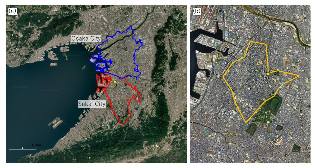
Figure 1 Aerial map of the Osaka metropolitan area, where blue and red represent the boundaries of Osaka city and Sakai city, respectively (a) and an enlarged view of the area surrounding the observation tower (b). The yellow star represents the location of the eddy covariance tower, and the orange line represents the mean position of the source area contributing 80 % to the flux footprint during the daytime (Ueyama and Takano, 2022). The map was obtained from © Google Earth.

Turbulent fluxes were calculated via the EC method using the flux calculator program version 2 (Ueyama et al., 2012). Before calculating the covariance, spikes in the raw data were removed, and then a double-rotation method was applied to set the mean vertical wind velocity to zero. High-frequency attenuation was corrected on the basis of an empirical transfer function (Moore, 1986) for CH₄ fluxes, whereas the theoretical transfer function was applied for other fluxes. Air density correction was applied for CH₄ fluxes (McDermitt et al., 2011) and CO₂ and water vapor fluxes (Webb et al., 1980). Quality controls were applied via stationary tests and higher-moment tests (Vickers and Mahrt, 1997). Nighttime data were not filtered on the basis of the friction velocity (Ueyama and Takano, 2022). To prevent flow distortion by the tower, we did not use flux data when the wind direction was from the tower (45–100°) (Okamura et al., 2024). Further details of the flux calculations are provided in previous studies (Takano and Ueyama, 2021; Ueyama and Takano, 2022).

To calculate daily and annual CH₄ fluxes, the data gaps were filled via the mean diurnal variation (MDV) method (Falge et al., 2001). Because the CH₄ fluxes were lower on weekends or holidays than on weekdays, the MDVs were determined separately for weekdays and weekends. To apply the MDV method, we used a 31 d moving window for weekdays and a 121 d moving window for weekends and holidays. The MDV method was conducted with 100 bootstrapping samples, and the mean and standard error of the bootstrapping were subsequently used for gap filling and their uncertainties, respectively. In this study, the measured fluxes from 1 January to 31 December 2023 were used for the analysis.

2.4 Water vapor corrections for the gas analyzer

According to a previous study (Commane et al., 2023), the gas analyzer used in this study requires a correction for the presence of water vapor. In this study, we used three analyzers of the same model (MIRA Ultra, Aries Technologies). We checked the response of the CH₄ and C₂H₆ concentrations to the water vapor concentration in the laboratory. The compressed air in the large-volume cylinders passed through the analyzer, and the water vapor concentration was changed by dehumidifying or humidifying with Nafion tubing (ME-110, Perma Pure LLC, USA). We obtained the following empirical relationships for the CH₄ and C₂H₆ concentrations:

• Analyzer 1

  $$\begin{array}{}\text{(1)}& \begin{array}{rl}{\mathrm{CH}}_{\mathrm{4}}\left({\mathrm{H}}_{\mathrm{2}}\mathrm{O}\right)=& -{\mathrm{2.07786}}^{-\mathrm{10}}\times X_{{\mathrm{H}}_{\mathrm{2}}\mathrm{O}}^{\mathrm{2}}\\ & +{\mathrm{4.0952}}^{-\mathrm{6}}\times X_{{\mathrm{H}}_{\mathrm{2}}\mathrm{O}}-\mathrm{0.020178}\end{array}\end{array}$$

• Analyzer 2

  $$\begin{array}{}\text{(2)}& {\displaystyle }\begin{array}{rl}{\mathrm{CH}}_{\mathrm{4}}\left({\mathrm{H}}_{\mathrm{2}}\mathrm{O}\right)=& -{\mathrm{3.2856}}^{-\mathrm{10}}\times X_{{\mathrm{H}}_{\mathrm{2}}\mathrm{O}}^{\mathrm{2}}\\ & +{\mathrm{8.4828}}^{-\mathrm{6}}\times X_{{\mathrm{H}}_{\mathrm{2}}\mathrm{O}}-\mathrm{0.05478}\end{array}\text{(3)}& {\displaystyle }{\mathrm{C}}_{\mathrm{2}}{\mathrm{H}}_{\mathrm{6}}\left({\mathrm{H}}_{\mathrm{2}}\mathrm{O}\right)={\mathrm{4.8243}}^{-\mathrm{5}}\times X_{{\mathrm{H}}_{\mathrm{2}}\mathrm{O}}-\mathrm{0.6521}\end{array}$$

• Analyzer 3

  $$\begin{array}{}\text{(4)}& \begin{array}{rl}{\mathrm{CH}}_{\mathrm{4}}\left({\mathrm{H}}_{\mathrm{2}}\mathrm{O}\right)=& {\mathrm{2.11169}}^{-\mathrm{11}}\times X_{{\mathrm{H}}_{\mathrm{2}}\mathrm{O}}^{\mathrm{2}}\\ & -{\mathrm{1.42907}}^{\mathrm{6}}\times X_{{\mathrm{H}}_{\mathrm{2}}\mathrm{O}}-\mathrm{0.020178}\end{array}\end{array}$$

where $X_{{\mathrm{H}}_{\mathrm{2}}\mathrm{O}}$ represents the water vapor concentration (ppm). CH₄ (H₂O) and C₂H₆ (H₂O) are the changes in the CH₄ and C₂H₆ concentrations, respectively, as a function of the water vapor concentration. For the mobile and atmospheric measurements, we corrected the effect of water vapor to values at water vapor concentrations of 10 000 ppm for analyzers 1 and 3 and 13 000 ppm for analyzer 2. For the C₂H₆ concentration, we only found a clear linear increase in water vapor for analyzer 2; water vapor correction was applied for analyzer 2 only, where the C₂H₆ value was corrected to 13 000 ppm water vapor.

2.5 Data analysis for mobile measurements

The CH₄ emission hotspots were identified via the data from the mobile measurements. For both the vehicle and bicycle measurements, hotspots were defined as locations where the CH₄ concentration was elevated by more than 0.1 ppm with respect to the local baseline concentration (hereafter referred to as CH₄ enhancement; ΔCH₄). The local baseline concentration was defined as the 5th percentile value during a 5 min moving window (i.e., a 2.5 min window on either side of a measurement point). Previous studies used median values from the length of the moving window, ±2.5 min (Maazallahi et al., 2020; Weller et al., 2019), but we have used the 5th percentile as a baseline, a compromise solution based on the methods described in Dowd et al. (2024) and Tettenborn et al. (2025). As the approximate baseline was 2.0 ppm CH₄ throughout the campaigns, the choice of baseline metric is not anticipated to have material impact on the overall results. In addition to ΔCH₄, the C₂H₆ enhancement (ΔC₂H₆) was calculated in the same manner and was used for estimating the source attributions of ΔCH₄. In accordance with a previous study that used the C₂H₆ : CH₄ (C₂ : C₁) ratio (Fernandez et al., 2022), we grouped the CH₄ hotspots into three categories: biogenic (C₂ : C₁ < 0.005), natural gas (0.005 < C₂ : C₁ < 0.1), and combustion (C₂ : C₁ > 0.1) sources. Although the C₂ : C₁ ratio for the natural gas distribution in Osaka is reported to be 0.076, we used a wider range of C₂ : C₁ ratios for the source attributed to natural gas owing to potential dilution by surrounding air. For the vehicle measurements, we eliminated the data when the vehicle speed was less than 1.5 km h⁻¹ to prevent possible contamination from vehicle exhaust during idling. The identified CH₄ enhancements were aggregated at a spatial resolution of 12 s in both latitude and longitude (approximately 471 m in longitude and 372 m in latitude) by obtaining the maximum CH₄ enhancement (hereafter referred to as a leak indication, LI) to avoid double counting of single LI. This spatial resolution was determined based on measurements showing that detected plumes sometimes extended over more than 200 m, and that the majority of distances between neighboring LIs exceeded this value. On the basis of the mean speed of the vehicle (17.0 km h⁻¹) and bicycle (9.7 km h⁻¹), approximately 22 and 38 measurement points were, on average, available for the vehicle and bicycle measurement analysis, respectively, within this spatial resolution.

To categorize the CH₄ LI intensity, we employed the emission magnitude categories defined in previous studies (Fernandez et al., 2022; von Fischer et al., 2017): low emissions (< 6 L min⁻¹), medium emissions (6–40 L min⁻¹), and high emissions (> 40 L min⁻¹). The emission rate was calculated via Eq. (5). These emission categories correspond to CH₄ enhancements of low emissions (< 1.6 ppm), medium emissions (1.6 to 7.6 ppm), and high emissions (7.6 ppm) in the empirical model by Weller et al. (2019). CH₄ emission estimates derived from LIs using the empirical model by Weller et al. (2019) showed considerable uncertainty in Osaka, as discussed below. Because the emission rates calculated for individual LIs may carry large uncertainties, expressing these values in standard emission units could be misleading. Therefore, we presented CH₄ enhancement relative to the baseline concentration (in ppm) for each emission category in addition to the emission (in L min⁻¹), ensuring consistency with the definitions used in previous studies.

Differences in CH₄ enhancements between the two types of gas analyzers at different heights were evaluated via vehicle measurements. On the basis of previous studies (von Fischer et al., 2017; Weller et al., 2019), CH₄ emissions are expected from underground pipes used in natural gas distribution. Furthermore, wind speeds are generally lower at lower measurement heights, resulting in less diluted emission plumes. Considering these assumptions, our high-priority gas measurements were performed at 0.5 m using a gas analyzer (Mira Ultra; the optical cavity is 60 cm³), but the measurements for 1.85 m were simultaneously examined with an LI-7810 analyzer (optical cavity is 6.41 cm³). We compared LIs with the two measurements to assess which heights effectively detected LIs, finding the tendency that CH₄ enhancements measured by Mira Ultra (0.5 m height) are larger than those by LI-7810 (1.85 m height) (see Sect. 3.1). Hereafter, the CH₄ measurements refer to those by Mira Ultra.

To estimate regional CH₄ emissions on the basis of mobile measurements, we applied scaling EC-derived daytime CH₄ fluxes to the city-scale fluxes using the mobile measurements and an empirical equation (Weller et al., 2019), extending the fluxes beyond the EC footprint to estimate CH₄ emissions at the city scale. This scaling method clarified the relationship between the results from empirical models and the regional CH₄ fluxes observed using the EC method, with the goal of spatial extrapolation. Since CH₄ fluxes measured by the EC method reflect both street-level emissions and sources located on building rooftops, walls, and other vertical surfaces, the scale factor may capture the relationship between street-level emissions and vertically integrated emissions at the city scale. This scaling method also quantified the differences between mobile and EC measurements, determining the extent to which ground-based mobile measurements deviate from the spatially representative EC results. Using the simplified approach, our objectives are to (1) quantify leaks and determine associated CH₄ emissions in Osaka, and (2) compare CH₄ emissions in a Japanese city with those in other cities whose CH₄ emissions are calculated via this equation (Vogel et al., 2024). In accordance with Weller et al. (2019), the CH₄ emission rate was calculated as follows:

$$\begin{array}{}\text{(5)}& \ln \left(\mathrm{Em}\right)=\left(\ln \right(C)+\mathrm{0.988})/\mathrm{0.817}\end{array}$$

where Em is the emission rate (L min⁻¹) and where C is the maximum CH₄ LI (ppm) within a grid. Here, Em was calculated on the basis of C measured. Using Em, the CH₄ fluxes were calculated as follows:

$$\begin{array}{}\text{(6)}& F_{{\mathrm{CH}}_{\mathrm{4}}}=A\times {\mathrm{Em}}_{\mathrm{mean}}\times \mathrm{Num}\times \mathrm{Dist}/\mathrm{Area}\end{array}$$

where $F_{{\mathrm{CH}}_{\mathrm{4}}}$ represents the CH₄ fluxes (nmol m⁻² s⁻¹), Em_mean represents the areal mean of Em within each ward or city, Num represents the detected hotspot count per travel distance (km⁻¹), Dist represents the total road length of the target ward or city (km), Area represents the area of the target ward or city (m²), and A represents the correction factor of the empirical estimates. For the total road length, we did not include the length of highways because highways are generally located over or along arterial roads. To account for uncertainties associated with limited measurements, Em_mean was calculated 100 times via bootstrap sampling from the measurements, and the mean and standard deviation of $F_{{\mathrm{CH}}_{\mathrm{4}}}$ were calculated from 100 bootstrapped samples. Equation (6) was applied to calculate $F_{{\mathrm{CH}}_{\mathrm{4}}}$ for each ward or city. This upscaling procedure was conducted for the respective biogenic and natural gas LIs and then summed for each flux. We did not upscale the combustion LIs because combustion was identified as a minor source of CH₄ in the measured data. This approach to estimating regional CH₄ emissions is widely adopted (Vogel et al., 2024; Weller et al., 2019) with the assumption that the spatial distribution of CH₄ emissions obtained from mobile measurements is representative of the emission patterns across the entire study area. This study evaluated the assumption by comparing upscaled CH₄ emissions derived from bicycle-based measurements (complete spatial coverage) with vehicle-based measurements (coverage only a portion of the area but are assumed to reflect the broader spatial characteristics). The total flux calculation was also performed for all LIs (not categorized). CH₄ fluxes upscaled by the two estimates (with and without source attributions) were compared to understand the uncertainties associated with the procedure. Note that a correction factor, A, close to 1 indicates low uncertainty, whereas a deviation from 1 suggests a larger correction with greater uncertainty in the estimates derived from mobile measurements.

To understand the uncertainties in upscaled regional fluxes, we further examined the different equations proposed by recent studies after Weller et al. (2019). Instead of using Eq. (5), the following equations were applied for evaluating CH₄ emissions:

$$\begin{array}{}\text{(7)}& {\displaystyle }\ln \left(\mathrm{Em}\right)=\left(\ln \right(C)+\mathrm{0.521})/\mathrm{0.795}\text{(8)}& {\displaystyle }\ln \left(\mathrm{Em}\right)=\left(\ln \right(C)+\mathrm{2.738})/\mathrm{1.329}\text{(9)}& {\displaystyle }\ln \left(\mathrm{Em}\right)=\left(\ln \right(C)+\mathrm{2.716})/\mathrm{0.741}\end{array}$$

Three equations were developed on the basis of a control experiment in Germany (Wietzel and Schmidt, 2023), South Korea (Joo et al., 2024), and Japan (Umezawa et al., 2025).

Upscaled CH₄ fluxes were aggregated at the ward or city scale for Sakai city and Osaka city. Fluxes from the vehicle and bicycle measurements were compared for Kita and Sakai wards of Sakai city, as well as for Sakai city. The comparison of CH₄ fluxes for Kita and Sakai wards could provide insight into how the coarse vehicle measurements were consistent with the intensive bicycle measurements that covered almost all streets. A comparison of CH₄ fluxes across Sakai city was conducted to assess how city-scale CH₄ fluxes differ in terms of spatial coverage between vehicle measurements (covering various urban landscapes) and bicycle measurements (covering only the city center and residential areas).

The total CH₄ emissions were calculated by multiplying the upscaled CH₄ fluxes to the city area and a factor for the temporal representation. Although mobile measurements were conducted in the daytime, we found that the CH₄ fluxes obtained via the EC method (Takano and Ueyama, 2021) clearly exhibited diurnal variation. To consider the diurnal variability, we multiplied the upscaled fluxes by 0.64, which was the ratio of the daily mean to the daytime mean flux (09:00–17:00 LT (local time)) in 2023, when calculating the daily fluxes. Based on the locations of emission point sources identified by mobile measurements (discussed in Sect. 3), CH₄ emissions across the study area were likely to exhibit diurnal variation. Although extrapolating the diurnal correction factor (0.64) introduces some uncertainty in regional CH₄ emissions, we applied the correction to avoid overestimations due to the absence of nighttime measurements. The daily fluxes were then summed over 365 d for the annual fluxes because CH₄ emissions during the seasons of October and November when the mobile measurements were conducted were similar to the annual mean (discussed with Fig. 10f). The annual emissions were only calculated for the vehicle measurements. Although bicycle measurements were also presented, their limited spatial coverage – restricted to the city center and residential areas – may underrepresent the influence of rural areas on regional CH₄ emissions.

On the basis of visual inspections of mobile measurement data, many LIs have been detected near restaurants. We quantified whether LIs were significantly more common near restaurants than others were. First, the probability of detecting restaurants near LIs, P(R|LI), was calculated, where the locations of the restaurants were obtained via two databases on gourmet websites: Yahoo (https://developer.yahoo.co.jp, last access: 10 December 2024) and Hot Pepper Gourmet by Recruit (https://www.hotpepper.jp/, last access: 10 December 2024). To use the databases, we used an application programming interface (API) provided by the companies. Because the two available databases did not fully cover all restaurants in the cities, we compared the probability that the CH₄ concentration significantly increased near restaurants. We identified whether restaurants were located within 80 m from an LI, and then the probability was calculated for Sakai city and Osaka city. The distance of 80 m was determined on the basis of visual inspection, considering the precision of the restaurant location in the database and the distance between roads and buildings. Then, a baseline probability was determined on the basis of five bootstrapping samples of randomly selected points that were not identified as an LI (i.e., the probability of a restaurant being within 80 m given that there is no detection, P(R|no LI)). Finally, we compared the probability of restaurants being located near LIs to that of the baseline. On the basis of Bayesian theory, we calculate the inverse probability of P(R|LI), namely, the probability that restaurants emit natural gas related to CH₄, P(LI|R), as follows:

$$\begin{array}{}\text{(10)}& {\displaystyle }P\left(\mathrm{LI}\right|R)=P(R\left|\mathrm{LI}\right)\times P\left(\mathrm{LI}\right)/P\left(R\right)\text{(11)}& {\displaystyle }P\left(R\right)=P\left(R\right|\mathrm{LI})\times P(\mathrm{LI})+P(R\left|\mathrm{no}\mathrm{LI}\right)\times P\left(\mathrm{no}\mathrm{LI}\right)\end{array}$$

where P(R) is the probability of existing restaurants within the 80 m sector, P(LI) is the probability of LIs existing within the 80 m sector, and P(no LI) is the probability of no LIs existing within the 80 m sector.

3 Results

3.1 Vehicle measurements

On the basis of the vehicle measurements, we surveyed 2558 km across the Osaka metropolitan area, mostly in Osaka city (1280 km) and Sakai city (1049 km), and identified 753 LIs (Fig. 2). Of the LIs, 233 were classified as biogenic sources, and 481 were classified as natural gas sources. Combustion sources were minor for our measurements (39 LIs). Ninety-five percent of the detected LIs were less than 1 ppm in enhancement, indicating that the detected LIs were mainly small leaks. Scatter plots between the CH₄ and C₂H₆ enhancements revealed that many of the CH₄ enhancements increased with increasing C₂H₆ concentration according to the gas supply ratio set by the local gas company (C₂ : C₁ = 0.076 ppm ppm⁻¹) (Fig. 3a). Furthermore, the data with a high C₂ : C₁ ratio were highly correlated at the local scale, where the red dots in Fig. 3 represent correlation coefficients between the two gases that were greater than 0.7 for the 5 min time frame. These results indicate that LIs that originate from a natural gas source can be correctly classified via C₂H₆. On the basis of visual inspection and smell during measurements near CH₄ enhancements, the interpretable reasons for CH₄ enhancement were sewage treatment plants, sewer pipes, plants for fermented foods, reservoirs, ditches of kofun (monument of an ancient emperor), river sides, dairy farms, composts, industrial plants, and various types of restaurants, including market streets. Unattributable enhancements were also measured in various land uses, such as residential, commercial, and industrial areas.

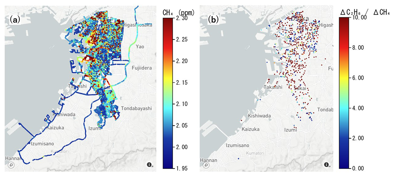
Figure 2 Spatial distributions of CH₄ concentrations (a) and identified leak indications (LIs) (b) on the basis of vehicle measurements. The color bar scale in panel (b) is the C₂ : C₁ ratio (ppb ppm⁻¹). Visualization was achieved using Plotly in Python, which uses © OpenStreetMap as a basemap provided by © mapbox.

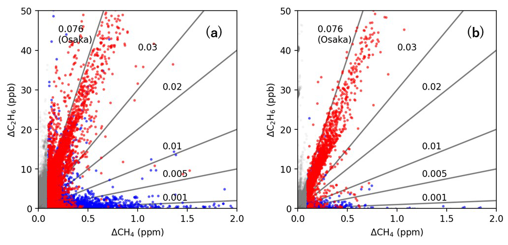
Figure 3 Relationships between CH₄ and C₂H₆ enhancements based on vehicle measurements (a) and bicycle measurements (b). The red dots represent the data for which the correlation coefficient between these two gases was greater than 0.7, and the blue dots represent the data for which the correlation coefficient was lower. Gray dots represent data that were not classified as leak indications because of the CH₄ enhancements smaller than the criteria (0.1 ppm). The lines represent various slopes, and 0.076 ppm ppm⁻¹ represents the C₂ : C₁ ratio for natural gas provided by the local gas company in the Osaka metropolitan area.

LIs per travel distance were 2 times greater in Osaka city (495 LIs; 0.39 km⁻¹) than in Sakai city (235 LIs; 0.22 km⁻¹). In terms of emission sources, both biogenic and natural gas LIs were higher in Osaka city (0.13 km⁻¹ for biogenic gas and 0.24 km⁻¹ for natural gas) than in Sakai city (0.05 km⁻¹ for biogenic gas and 0.15 km⁻¹ for natural gas). These results indicate that Osaka city, which is more urbanized than Sakai city, has more natural gas and biogenic CH₄ emission points.

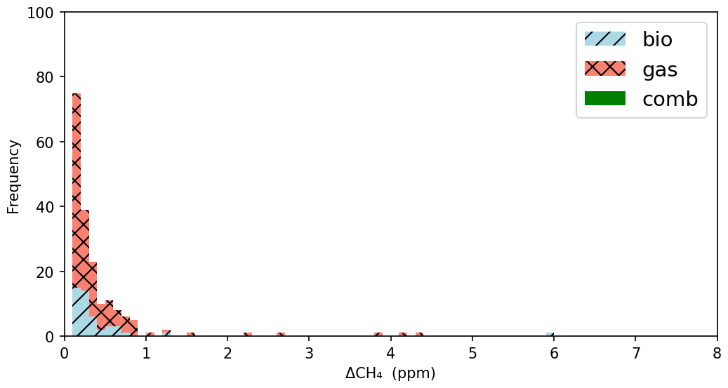
The intensities of LIs were generally low, where 733 out of 753 LIs (i.e., 97.3 %) were classified into a low category (i.e., less than 1.6 ppm enhancement or 6 L min⁻¹ emissions) (Fig. 4). There was no high-emission category (i.e., greater than 7.6 ppm enhancement or 40 L min⁻¹ emissions) in Osaka and Sakai cites. Twenty LIs were categorized as middle. The highest LI (7.57 ppm enhancement or 39.9 L min⁻¹ emissions) was observed near compost in croplands in the rural area of Sakai city, which was identified as a biogenic source. The second to fourth highest enhancements (6.5 to 5.4 ppm, respectively; 33 to 26 L min⁻¹ emissions, respectively) were natural gas sources in Osaka city, which were observed at a narrow street in a residential area or at a main street in a commercial area. The second highest biogenic enhancement (4.39 ppm or 20 L min⁻¹ emission) was detected in the bay area. Note that emissions (L min⁻¹) presented were calculated using Eq. (5).

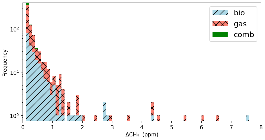
Figure 4 Histogram of CH₄ enhancements (ΔCH₄) based on vehicle measurements for Osaka and Sakai. Note that the y-axis is shown as a log scale. The values 1 to 8 in the horizontal axis for ΔCH₄ correspond to emission rates of 3.4, 7.8, 12.9, 18.3, 24.0, 30.0, and 36.3 L min⁻¹, respectively.

The detected numbers of LIs and ΔCH₄ were greater in the Mira Ultra gas analyzer, whose inlet was installed at 0.5 m, than in the LI-7810 analyzer, whose inlet was installed at 1.85 m (Fig. A2), where comparisons were made when the CH₄ concentrations were measured by both analyzers. The estimated LIs were 723 for Osaka and Sakai cities in terms of the measurements by the Mira Ultra analyzer, but those by the LI-7810 analyzer were 646. The underestimation of the number of LIs by the LI-7810 analyzer was more significant for biogenic sources (130 for LI-7810 and 221 for Mira Ultra) than for natural gas sources (370 for LI-7810 and 468 for Mira Ultra). Combustion sources were also more effectively detected by the Mira Ultra analyzer (34) than the LI-7810 analyzer (6). The maximum and median ΔCH₄ values were 7.6 and 0.20 ppm, respectively, for the Mira Ultra analyzer, whereas those for the LI-7810 analyzer were 3.4 and 0.14 ppm, respectively.

3.2 Bicycle measurements

The bicycle measurements provided characteristics similar to those obtained from the vehicle measurements (Fig. 5). The bicycle measurements provided a detailed view of CH₄ concentrations and LIs with high density, which covered almost all streets, including very narrow streets and dead ends that could not be accessed by a vehicle (Fig. A3). Many CH₄ enhancements were evident in the C₂ : C₁ ratio according to the local natural gas company (Fig. 3b), which was consistent with the vehicle measurements (Fig. 3a).

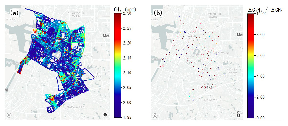
Figure 5 Spatial distributions of CH₄ concentrations (a) and identified leak indications (LIs) (b) on the basis of bicycle measurements. To remove the daily variations in the CH₄ concentration for visualization, the CH₄ concentrations were rescaled so that the 5th percentile of the CH₄ concentration on each measurement day was 2.0 ppm; this rescaling was performed only for visualization and not as part of the data processing and analysis. Visualization was achieved using Plotly in Python, which uses © OpenStreetMap as a basemap provided by © mapbox.

The number of identified LIs was 187 per 1162 km from the north to the central part of Sakai city (Fig. 6). The LI density (0.16 km⁻¹) was similar to that obtained from the vehicle measurements for the same area (0.25 km⁻¹ when including combustion LIs or 0.23 km⁻¹ when not including combustion LIs). Compared with the vehicle measurements, the percentage of natural gas CH₄ LIs (75 %) was greater in the bicycle measurements than in the vehicle measurements (64 %). As with the vehicle measurements, there was no LI categorized as high, and 181 out of 187 LIs were categorized as small. The highest LI was 5.9 ppm (29 L min⁻¹ emission), which was identified as a biogenic source near a fermented food factory. The second and third highest LIs were observed near a building at Osaka Metropolitan University (4.3 ppm enhancement or 20 L min⁻¹ emission) and at a narrow street in a residential area (4.2 ppm enhancement or 10 L min⁻¹ emission), respectively, which were identified as natural gas sources. There was no LI categorized as combustion on the basis of the bicycle measurements.

Figure 6 Histogram of CH₄ enhancements (ΔCH₄) based on bicycle measurements for Sakai.

3.3 Restaurants and sewage treatment plants

The probability of a restaurant existing near identified natural gas LIs was significantly greater than that near a location where no natural gas LI was observed (hereafter referred to as the baseline probability) (Fig. 7). For Sakai city, the probability of a restaurant being included in the vehicle measurements was 14 %, and the probability of a restaurant being included in the bicycle measurements was 20 %, which was significantly greater than the baseline probability (4.7 % ± 0.8 % for the vehicle measurements and 8.8 ± 0.4 % for the bicycle measurements; plus/minus sign denotes standard error of bootstrapping). The probability of a restaurant existing near natural gas LIs was 30 % for Osaka city, which was higher than that for Sakai city. The baseline probability for Osaka city (22 % ± 1.4 %) was also higher than that for Sakai city because Osaka city is a highly urbanized city where there are many restaurants. On the basis of Bayesian theory, the probabilities of existing restaurants emitting natural gas-related CH₄ were 2.4 % for Osaka city, 2.5 % for Sakai city according to vehicle measurements, and 2.7 % for Sakai city according to bicycle measurements. This finding either suggests that 2 %–3 % of restaurants have detectable gas leaks or that if all restaurants emit CH₄, they only emit detectable levels (detectable at the roadside) 2 %–3 % of the time.

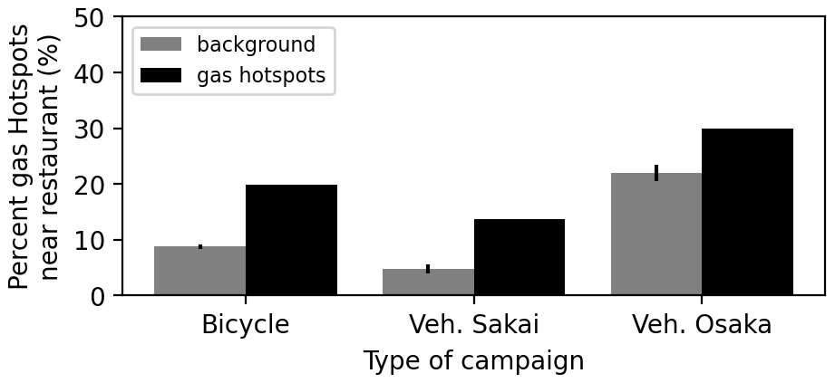
Figure 7 Probability of a restaurant existing near identified natural gas LIs and that near a location where no natural gas LI was identified. The error bars represent the standard errors for bootstrapped samples randomly obtained from the mobile measurement data where natural gas LIs were not identified.

CH₄ enhancements near sewage treatment plants were not too high, i.e., up to 4.3 ppm (Fig. A4). Although the C₂ : C₁ ratio revealed that most of the CH₄ enhancements were biogenic (n = 11), four plants with high C₂ : C₁ ratios (Chisima, Nakahama, Tsumori, and Chubu Mizumirai) were classified as having natural gas emissions.

3.4 Eddy covariance measurements

The CH₄ fluxes measured via the EC method clearly exhibited diurnal variations throughout the seasons (Fig. 8). The daytime CH₄ emissions were higher than the nighttime CH₄ emissions throughout the seasons. Although nighttime CH₄ fluxes were consistent across seasons with an average of 26 nmol m⁻² s⁻¹, daytime fluxes were lower in spring compared to other seasons (Fig. 8). Wind sector analysis for daytime fluxes revealed higher CH₄ emissions in the WSW, N, and NNW sectors during summer (Fig. 9a), as found by a previous study conducted in 2019 (Takano and Ueyama, 2021). These elevated emissions may be attributed to anthropogenic sources, such as high industrial-commercial development and extensive major road networks (Ueyama and Ando, 2016; Okamura et al., 2024), and presumably to sewage treatment plants in these wind sectors (Takano and Ueyama, 2021). A similar pattern of elevated daytime CH₄ fluxes in the same three wind sectors was observed in winter, although the magnitudes were lower than those in summer (Fig. 9b). The seasonal variations in CH₄ fluxes showed two peaks in the year, one where summer emissions were highest and a smaller peak in winter (Fig. 8f). The CH₄ fluxes were greater on weekdays (46 nmol m⁻² s⁻¹) than on weekends and holidays (34 nmol m⁻² s⁻¹), especially during the daytime (72 nmol m⁻² s⁻¹ on weekdays and 50 nmol m⁻² s⁻¹ on weekends and holidays) (Fig. 8e). The annual CH₄ emissions in 2023 according to the EC measurements were 14.2 ± 1.3 g CH₄ m⁻² yr⁻¹ (plus/minus sign represents the standard error associated with the gap-filling).

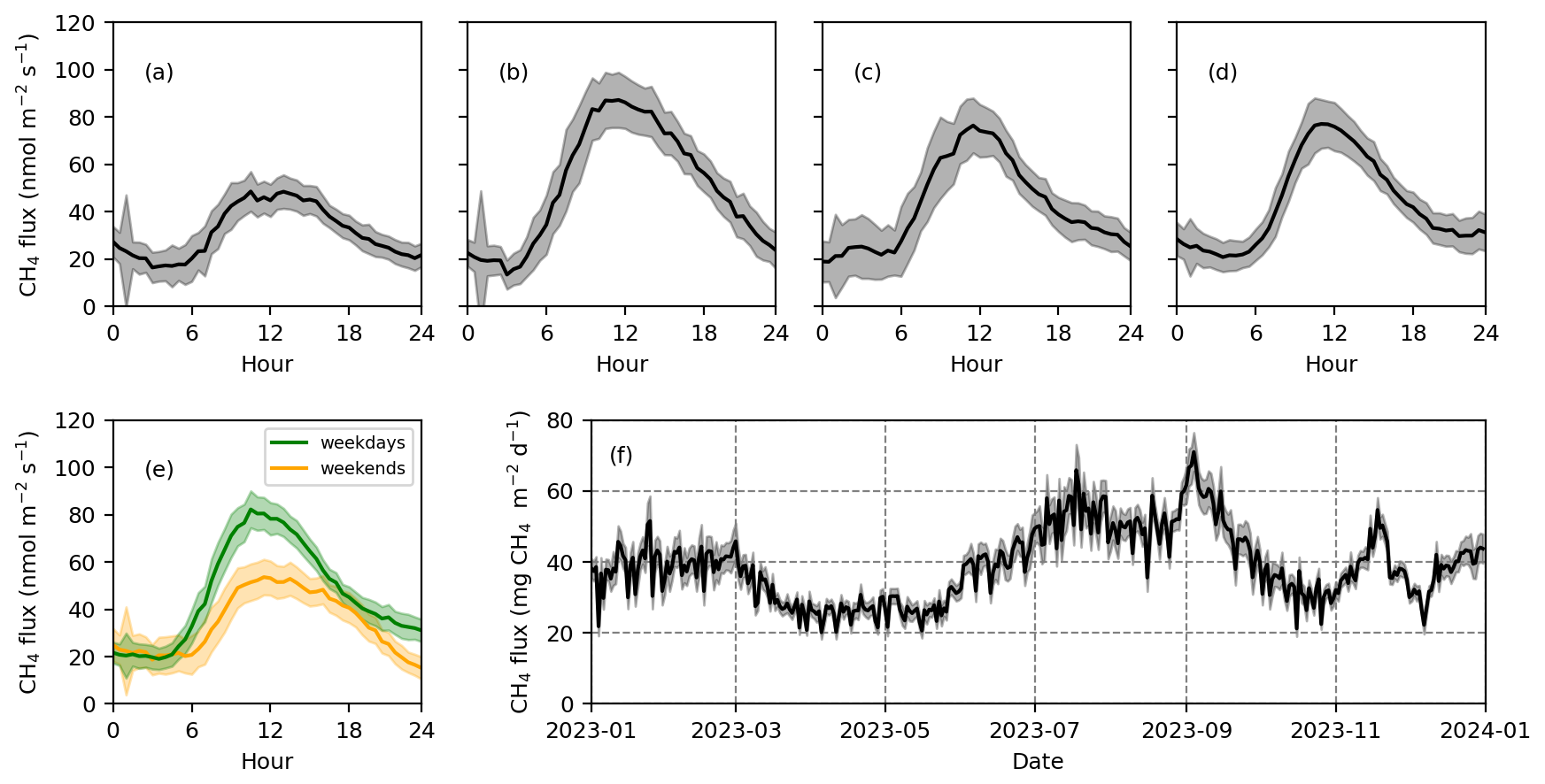
Figure 8 CH₄ fluxes measured via the eddy covariance method in 2023. Mean diurnal variation in CH₄ fluxes from March to May (a), from June to August (b), from September to November (c), from December to February (d), and for the whole year for weekdays and weekends (e). The shading in panels (a)–(e) indicates the standard error of the measured CH₄ fluxes at each time point. The daily CH₄ flux for 2023, where the shading represents the standard error based on 100 bootstrap samples in gap filling (f).

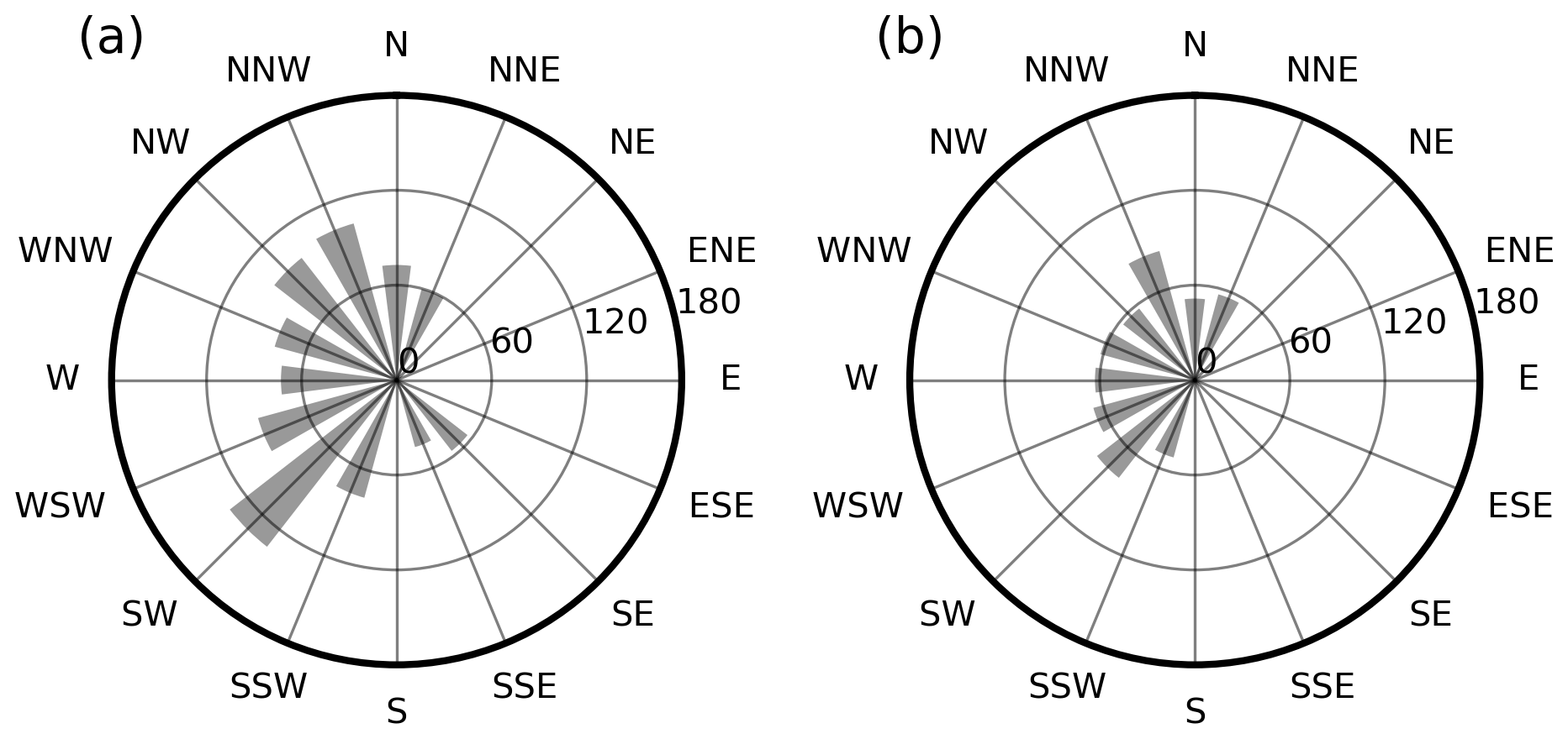
Figure 9 Stacked charts of half-hourly CH₄ fluxes (nmol m⁻² s⁻¹) during the daytime (09:00–17:00 LT) for the 22.5° wind sector in (a) summer (June–September) and (b) winter (December–March) of 2023.

3.5 Regional CH₄ fluxes and emissions

On the basis of the detected LIs combined with the empirical equations (Eqs. 5 to 9), CH₄ fluxes were estimated from mobile measurements for the same region covered by the EC flux footprint. Using Eq. (5), the aggregate CH₄ emissions from the Sakai flux footprint were estimated to be much smaller than the EC flux, giving a scale factor A of 22 (Eq. 6). Alternative scale factors of A = 38 for Eq. (7), A = 10 for Eq. (8), and A = 1.9 for Eq. (9) were also derived to match the EC flux. The different estimates of Em and associated differences in A could be caused by assumptions made in the control experiments.

The aggregate emissions estimate from the mobile measurements is representative of different emission processes (street-level emissions) to the total flux footprint from eddy covariance. Therefore, we do not expect the resulting emission totals to be directly comparable since it is likely the mobile measurements may miss emissions occurring above street level, as well as any smaller more disperse sources that do not result in a detectable sharp peak in the CH₄ concentration. However, the mobile measurements provide a much greater coverage of the city than the EC flux. As such, we use the mobile measurement estimates, adjusted by the derived scale factor, A, as a proxy to estimate CH₄ emissions across Sakai and Osaka cities, including the attribution to biogenic and natural gas sources. We estimated the upscaled CH₄ fluxes using Eq. (6) with different values of Em derived from Eqs. (5), (7), (8), and (9) and considered the range of upscaled fluxes as an uncertainty.

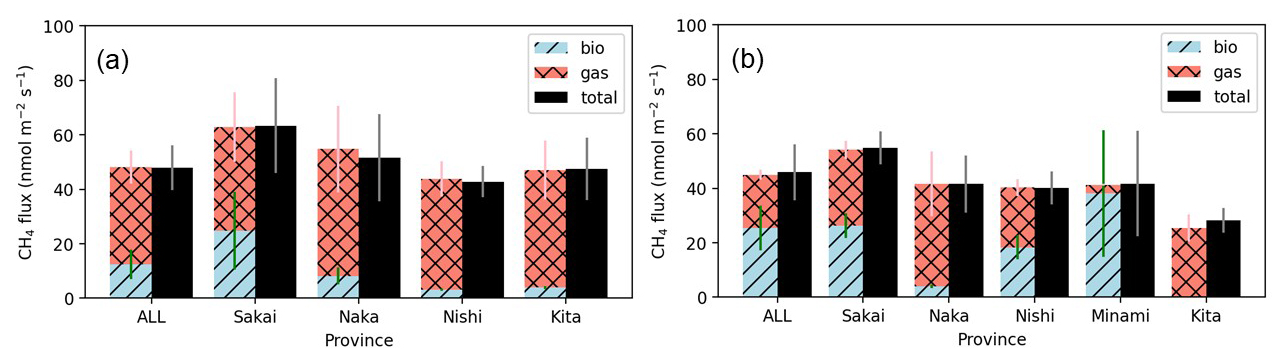
Figure 10 Upscaled CH₄ fluxes for Sakai city in terms of the entire city and each ward based on the bicycle measurements (a) and the vehicle measurements (b) using Eq. (5). The error bars represent the standard deviation based on bootstrapped samples.

CH₄ fluxes were estimated for the administrative divisions of Sakai city to compare the fluxes determined from the bicycle and vehicle measurements. As noted above, the estimated CH₄ fluxes were scaled to ensure that the upscaled CH₄ fluxes for Sakai Ward from the bicycle measurements were consistent with the long-term mean daytime CH₄ fluxes measured via the EC method (approximately 65 nmol m⁻² s⁻¹) (Sects. 3–4). There was no clear difference in CH₄ flux between estimates based on the sum of biogenic and natural gas fluxes and direct estimates without considering the source types (Fig. 10).

The estimated CH₄ fluxes for Sakai city were 51 ± 5 nmol m⁻² s⁻¹ according to the bicycle measurements and 49 ± 10 nmol m⁻² s⁻¹ according to the vehicle measurements. Hereafter, the value and plus/minus sign of the regional flux represent the mean and standard deviation of the fluxes upscaled by four different equations (Eqs. 5, 7, 8, and 9), respectively. Both estimates were generally similar, although different spatial representations and densities of the measurements were used. The bicycle measurements did not cover Minami and Mihara wards completely and covered only a few km for Higashi and Nishi wards. In contrast, vehicle measurements were missing data for only Mihara Ward. In addition to the city-scale fluxes, fluxes for each ward were also consistent between the bicycle and vehicle measurements, except for Kita Ward, where CH₄ fluxes were lower in the vehicle measurements (35 ± 15 nmol m⁻² s⁻¹) than in the bicycle measurements (50 ± 7 nmol m⁻² s⁻¹).

Although the total fluxes were consistent between the bicycle and vehicle measurements, the components of the fluxes, namely, the biogenic and natural gas fluxes, differed (Fig. 10). The biogenic fluxes were greater in the vehicle measurements than in the bicycle measurements, whereas the natural gas fluxes were the opposite. On the basis of the bicycle measurements, the biogenic and natural gas CH₄ fluxes for Sakai city were 13 ± 1 and 38 ± 4 nmol m⁻² s⁻¹, respectively, indicating that natural gas fluxes explained 75 % of the total CH₄ flux. For vehicle measurements, natural gas fluxes explained 47 % of the total CH₄ flux: 25 ± 1 nmol m⁻² s⁻¹ for biogenic fluxes and 23 ± 9 nmol m⁻² s⁻¹ for natural gas fluxes.

Among Sakai, Naka, and Kita wards, which were measured via both bicycle and vehicle measurements, biogenic fluxes tended to have greater contributions in Sakai Ward than in the other wards, which was consistent between the two measurements. The high contributions of biogenic sources could be explained by the combined sewer systems that remain in Sakai Ward but not in other wards in Sakai city. Furthermore, this result may be explained by the presence of Sakai city's largest sewage treatment plant in Sakai Ward. The high contributions of biogenic fluxes in Minami Ward (Fig. 10b) were associated with CH₄ fluxes from compost, dairy farms, and reservoirs because Minami Ward is the most rural place in Sakai city. For Nishi Ward, the bicycle measurements underrepresented the CH₄ fluxes owing to collecting data over 62 km.

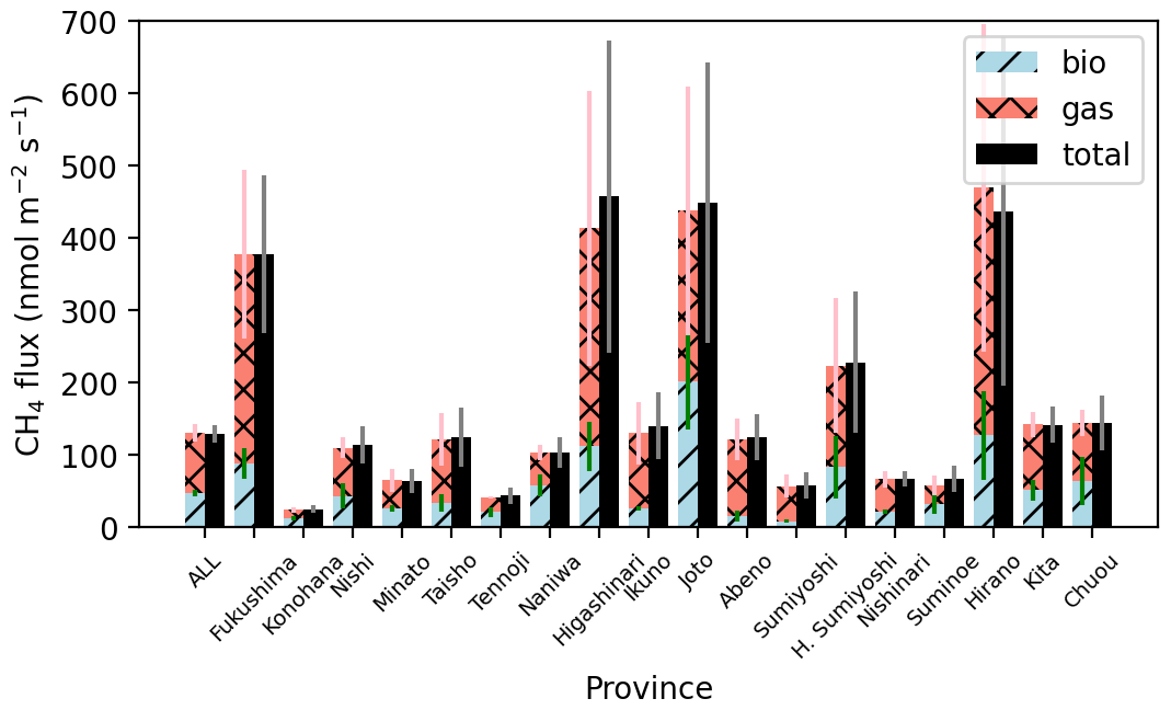
Figure 11 Upscaled CH₄ fluxes for Osaka city in terms of the entire city and each ward based on vehicle measurements using Eq. (6). The error bars represent the standard deviation based on bootstrapped samples.

The upscaled CH₄ fluxes for Osaka city (138 ± 14 nmol m⁻² s⁻¹) were 2.8 times greater than those for Sakai city (Fig. 11). The four high CH₄ fluxes were estimated for Fukushima, Higashinari, Joto, and Hirano wards. Fukushima Ward is the commercial and industrial area near Umeda station, the largest train station in Osaka Prefecture. Fukushima Ward has the second largest sewage treatment plant in terms of treatment capacity (326 000 m³ d⁻¹) in Osaka city. Joto and Higashinari wards are the second (29 183 km⁻²) and third (18 727 km⁻²) most densely populated areas in Osaka Prefecture. Except for Konohana and Tennoji wards, the CH₄ fluxes in wards in Osaka city were higher than those in Sakai city. For Osaka city, biogenic and natural gas fluxes contributed almost equally to the total CH₄ fluxes. On the basis of the vehicle measurements, the contributions of natural gas fluxes were greater in Osaka city (64 %) than in Sakai city (47 %).

The scaled annual CH₄ emissions, which were calculated via the CH₄ fluxes, the area of the city, and temporal correction, resulting in 10 021 ± 1000 t CH₄ yr⁻¹ for Osaka city and 2379 ± 480 t CH₄ yr⁻¹ for Sakai city on the basis of the vehicle measurements. These values were equivalent to the annual area-weighted fluxes of 44 ± 4 t CH₄ km⁻² yr⁻¹ for Osaka city and 16 ± 3 t CH₄ km⁻² yr⁻¹ for Sakai city. The biogenic emissions were 3632 ± 480 t CH₄ yr⁻¹ for Osaka city and 1191 ± 47 t CH₄ yr⁻¹ for Sakai city, whereas the natural gas emissions were 6389 ± 520 t CH₄ yr⁻¹ for Osaka city and 1188 ± 433 t CH₄ yr⁻¹ for Sakai city. If calculated based on bicycle measurements, CH₄ emissions for the entire Sakai city were extrapolated to 2472 t CH₄ yr⁻¹, although the rural Minami Ward was underrepresented. Of the total CH₄ emissions, natural gas sources accounted for 1852 t CH₄ yr⁻¹, while biogenic sources contributed 620 t CH₄ yr⁻¹. Biogenic emissions were lower than those derived from the vehicle measurements, likely due to the limited bicycle coverage of suburban areas (i.e., Minami Ward). In contrast, the high natural gas CH₄ emissions may reflect dense coverage of the city-center emissions by bicycle. It is worth noting that the annual emissions corrected the flux ratio between the daytime mean and daily mean (0.64) based on the ratio of daily mean to daytime of the CH₄ fluxes measured via the EC method (Sects. 2–5).

4 Discussion

The annual CH₄ emissions in Osaka (10 021 ± 1000 t CH₄ yr⁻¹) and Sakai (2379 ± 480 t CH₄ yr⁻¹) according to the vehicle measurements were considerably higher than those reported by the local government: 560 t CH₄ yr⁻¹ for Osaka city in 2021 (https://www.city.osaka.lg.jp/kankyo/cmsfiles/contents/0000352/352849/2022jimujigyouhen(1--5).pdf, last access: 10 December 2024) and 905 t CH₄ yr⁻¹ for Sakai city in 2020. Our estimates of CH₄ emissions were 18 times greater for Osaka and 2.6 times greater for Sakai than for the above emission reports. According to reports from local governments, CH₄ emissions from wastewater treatment account for 98 % of the total CH₄ emissions in Osaka city and 16 % of the total CH₄ emissions in Sakai city. The current measurements indicate that potentially unaccounted biogenic sources (sewer pipes, plants for fermented foods, reservoirs, ditches of ancient tombs, river sides, dairy farms, and composts) were also present in addition to wastewater treatment plants. In Sakai city, a coastal industrial zone is situated near the port area, and the local emission inventory indicates that combustion-related emissions from industrial facilities account for 62 % of the city's total CH₄ emissions. The measurements also revealed that natural gas-related sources accounted for 64 % of the total in Osaka city and 47 % of the total in Sakai city (75 % according to the bicycle measurements). Note that the 47 % estimated from the mobile measurements in Sakai does not reflect the major point sources associated with coastal industrial facilities. CH₄ emissions from these natural gas sources are currently not accounted for in the reports of the local government, resulting in considerable underestimates of CH₄ emissions.

The estimated natural gas CH₄ emissions (6389 ± 520 t CH₄ yr⁻¹ in Osaka and 1188 ± 433 t CH₄ yr⁻¹ in Sakai) were comparable to or even higher than those reported for European and North American countries. Vogel et al. (2024) reported that CH₄ emissions in 12 cities were in the range 50–5000 t CH₄ yr⁻¹, roughly corresponding to fluxes of 1–8 t CH₄ km⁻² yr⁻¹. The natural gas emissions for Osaka city (28 ± 2 t CH₄ km⁻² yr⁻¹) were greater than this range, and those for Sakai city (8 ± 3 t CH₄ km⁻² yr⁻¹) were in the middle to high range. Compared with previous studies in European and North American countries, the emission characteristics were different. The CH₄ LIs for Osaka and Sakai were mostly characterized by low enhancements, but the density of LIs was much greater than that reported in previous studies. This result indicated that a number of small CH₄ sources contributed to the total fluxes, whereas no large emission sources were found in our measurements. Vogel et al. (2024) reported that the top 10 % of emissions accounted for 60 %–80 % of the total emissions in European and North American countries, which contrasts with our results in Japan. Notably, without the adjustment using the EC measurements (i.e., when A = 1.0 was applied in Eq. 6), the natural gas CH₄ emissions (158 to 3395 t CH₄ yr⁻¹ in Osaka and 25 to 465 t CH₄ yr⁻¹ for Sakai, where ranges are based on four different empirical equations) were similar to those for the European and North American cities, where previous studies did not apply this correction. We discuss the uncertainties associated with this correction later. Even without the adjustment, the natural gas emissions in Osaka city according to the mobile measurements ranged from 25 % according to Eq. (7) to 606 % according to Eq. (9) of the total CH₄ emissions from Osaka city according to the inventory and were far greater than the inventory-based CH₄ emissions subtracted by the contribution of sewage (12 t CH₄ yr⁻¹).

The current measurements indicate that restaurants are an important CH₄ source co-emitting C₂H₆. One possibility for the emissions was the use of cast iron stoves for cooking in restaurants, where there may be unintentional gas leakage during on/off pulses (Lebel et al., 2022) because stoves that use natural gas are lit manually. Current duplicated measurements in a market street revealed that LIs were detected during the daytime but not during the early morning hours before restaurants were open. These results suggest that LIs from restaurants are not associated with steady gas leakage from pipelines but are related to intermittent leakage during gas use. The results further suggest that introducing built-in electronic ignition could reduce CH₄ emissions from restaurants in Japan. Lebel et al. (2022) reported that stoves using pilot lights resulted in considerably high CH₄ emissions for residential homes in the USA. CH₄ emissions from restaurants were not previously reported via mobile measurements in North American and European cities. The detection of CH₄ emissions near restaurants could be partly associated with narrow streets in Japanese cities. In the current vehicle measurements, the distance between the air inlet and restaurants near roads is approximately 2 m on narrow streets, 4 m on 1 lane roads on each side, and 5–9 m on the main roads. The close distance between the air inlet and restaurants could contribute to the effective detection of CH₄ enhancements.

The EC measurements revealed that CH₄ emissions underwent a clear diurnal variation (Fig. 8), where nighttime emissions were low, but emissions increased during the day. These results indicate that estimating CH₄ emissions via daytime mobile measurements might be overestimated if diurnal variations in LIs are not accounted for. On the basis of EC measurements (Gioli et al., 2013; Helfter et al., 2016; Huangfu et al., 2024; Pawlak and Fortuniak, 2016), similar diurnal variations were also observed in European and Chinese cities, although the ranges in the diurnal variations were greater in Sakai than in other cities (Huangfu et al., 2024). The nighttime emissions in Sakai were comparable to those measured in Łódź (20–25 nmol m⁻² s⁻¹) but lower than those measured in other cities (100 nmol m⁻² s⁻¹) in London (Helfter et al., 2016), Florence (Gioli et al., 2013), and Beijing (Huangfu et al., 2024). A small nighttime CH₄ flux could suggest that steady gas leaks are minimal in Sakai, as CH₄ emissions would be high at night if steady gas leaks were more significant. The daytime increase in CH₄ fluxes could be associated with increased human activities. The daytime fluxes were greater than those in Łódź (30–35 nmol m⁻² s⁻¹) but lower than those in London (150–200 nmol m⁻² s⁻¹), Florence (170 nmol m⁻² s⁻¹), and Beijing (200 nmol m⁻² s⁻¹).

The two seasonal peaks observed in summer and winter (Fig. 8) can be attributed to increased gas demand associated with high and low temperatures, respectively. Within the study area, gas demand rose in summer when daily air temperatures exceeded 20 °C, and similarly, in winter, demand increased as daily temperatures dropped. Natural gas consumption increased during both summer and winter, with summer usage being higher than winter usage, as observed at both the study site (Fig. S9 in Ueyama and Takano, 2022) and at university buildings in Sakai (Fig. A3 in Ueyama and Ando, 2016). Consequently, the CO₂ flux measured at this site exhibited a similar seasonal pattern, characterized by two distinct peaks (Ueyama and Ando, 2016; Ueyama and Takano, 2022). This gas demand could contribute to the seasonal variation in CH₄ flux. Other possible CH₄ sources in the summer include biogenic sources, such as sewage manholes and ditches surrounding ancient tombs (Takano and Ueyama, 2021). Detailed flux footprint analysis suggested that daytime CH₄ fluxes were influenced by a sewage treatment plant located in the bay area (Takano and Ueyama, 2021). Since the diurnal cycle of the dominant wind direction was controlled by land–sea breezes throughout the year (Fig. A1 in Ueyama and Ando, 2016), seasonal differences in the flux footprint likely had a limited influence on the seasonal variations in CH₄ flux.

Daytime CH₄ fluxes measured by the EC method varied with wind direction (Fig. 9). Elevated fluxes from the NNW and WSW directions showed a pattern consistent with observations in 2019 (Takano and Ueyama, 2021), suggesting a persistent trend at this site. Westerly winds, which are prevalent during the day due to the sea breeze, were coincident with elevated CH₄ fluxes. To the west of the tower site lie commercial and industrial zones with major roads, which have previously been linked to increased CO₂ fluxes (Ueyama and Ando, 2016) and NO₂ fluxes (Okamura et al., 2024) under similar wind conditions. This pattern suggests that CH₄ emissions may originate from such urban landscape. The wastewater treatment facilities are located near the outer edge of the source areas contributing 80 % of the turbulent fluxes. Therefore, they may also contribute to the observed CH₄ emissions, and fluxes from the northwest and southwest may be influenced by plumes emitted from these facilities (Takano and Ueyama, 2021).

A comparison of CH₄ emissions between Osaka and Sakai indicated that urban intensity increased CH₄ emissions and decreased contributions to biogenic emissions. The biogenic and natural gas CH₄ emissions in Osaka city were more than 2.8 and 3.8 times higher than those in Sakai city, respectively. Human activities, such as the use of natural gas and sewage water, could cause high emissions in highly urbanized cities, such as Osaka city. The use of natural gas in Osaka city is 3.4 times greater than that in Sakai city. The number of sewage treatment plants visited in Osaka city was 1.8 times greater than that visited in Sakai city in terms of treatment capacity. These gradients of urban intensity could explain the differences in CH₄ emissions among cities in Japan. Measurements in rural areas in Sakai (i.e., Minami Ward in Sakai city) indicated that biogenic sources, such as dairy farms, composts, and reservoirs, played an important role in regional CH₄ emissions. This suggests that biogenic CH₄ emissions could be important in rural areas in Japan.

A comparison of the vehicle and bicycle measurements revealed that the total CH₄ emissions did not differ substantially. This result indicates that vehicle measurements, albeit with limited coverage, are useful for estimating urban CH₄ emissions in Japan. In contrast, the source attributions differed between the two measurements. This inconsistency could be explained by the research design. We prioritized visiting known biogenic sources, such as sewage treatment plants, in the vehicle measurements, resulting in high bias in biogenic sources. For the natural gas CH₄ LIs, the LI densities were greater in the vehicle measurements (0.19 km⁻¹) than in the bicycle measurements (0.12 km⁻¹) for the same area (Kita, Sakai, and Naka wards). These results indicate that greater natural gas CH₄ emissions occurred in streets accessible to vehicles with higher levels of human activity, and biases for not covering narrow streets did not cause underestimates for natural gas LIs.

We stress that mobile measurements could underestimate CH₄ emissions from sewage treatment plants because the detected CH₄ enhancements were generally small (Fig. A4). The current study did not intend to improve estimates of large point sources that were already accounted for in the local government reports but rather aimed to identify the missing sources. The underestimates could be associated with the distance to emission sources in a sewage treatment plant (e.g., sedimentation pond and exposure tanks) from public roads where the measurements were made. CH₄ can be emitted at high altitudes (e.g., smokestacks), and these emissions may not be detected by mobile measurements on the ground. CH₄ emissions measured via the EC method were found to be greater when the flux footprint consisted of sewage treatment plants in Sakai (Takano and Ueyama, 2021). These results suggested that sewage treatment plants are important CH₄ sources, as accounted for in the reporting of the local government. Sewage treatment plants in Japanese megacities – including all plants examined in this study – primarily employ the activated sludge process for wastewater treatment. In addition, these plants typically use anaerobic digestion for sludge treatment, a process that is known to emit more CH₄ than systems without anaerobic digestion (Song et al., 2023). Experiments conducted at sewage treatment plants have shown that significant amounts of CH₄ are emitted during the sludge dewatering process and from storage tanks containing digested sludge (Oshita et al., 2014). Consequently, the CH₄ emissions in the current study were considerably underestimated or even did not account for these sources. Repeated measurements around point sources could improve the accounting of CH₄ emissions for point sources by inversely applying plume models (Stadler et al., 2022). The high C₂ : C₁ ratios measured near the sewage treatment plants might indicate the occurrence of combustion processes in the sewage treatment plants.

Simultaneous measurements of the two different inlet heights of the vehicle revealed that a low measurement height effectively detected LIs. These findings suggest that lower measurement heights are suitable for detecting urban CH₄ emissions in Japanese cities. In previous studies that conducted mobile measurements (Vogel et al., 2024), inlets were mostly installed at the front bumper or top of the roof, where the inlet heights were, for example, 0.5 m (Maazallahi et al., 2020); 0.6 m (Fernandez et al., 2022); 1.3 m (Takano and Ueyama, 2021); 2 m for bicycles and 2.5 m for vehicles (Ars et al., 2020); and 3 m (Phillips et al., 2013). The effective height could differ in each city depending on the emission strength and major source type. This highlights the need for consistent methodologies across study teams conducting this type of work, or at the very least, the development of transfer functions between instruments and mounting positions. A better understanding of the effective inlet height in a target city or country would improve estimates of urban CH₄ emissions.

Simultaneous measurements of CH₄ and C₂H₆ concentrations enabled us to understand the source attributions of CH₄ emissions. Two clear clusters in the C₂ : C₁ ratio separating biogenic and natural gas sources were observed in the current mobile measurements (Fig. 3), where the C₂ : C₁ ratios for natural gas sources almost coincided with those for natural gas by the local gas company. This result suggests that the measurements sufficiently captured the emission plume before it became substantially diluted, although the slope was a somewhat smaller C₂ : C₁ ratio than those distributed by the local gas company. Previously, source attributions were determined via simultaneous measurements of C₂H₆ concentrations (Fernandez et al., 2022; Hopkins et al., 2016; Maazallahi et al., 2020) and the isotopic composition of CH₄ (Fernandez et al., 2022; Defratyka et al., 2021; Maazallahi et al., 2020; Phillips et al., 2013).

In this study, upscaled fluxes and areal emissions were adjusted based on CH₄ fluxes measured via the EC method accounting for the differences between daytime CH₄ fluxes and diurnal variations in fluxes. This scale factor adjustment was necessary because empirical models (Weller et al., 2019; Wietzel and Schmidt, 2023; Joo et al., 2024; Umezawa et al., 2025) were much lower than the CH₄ flux measured via the EC method. The discrepancies in the empirical models in the Osaka metropolitan area might be explained by different emission characteristics between Osaka and the corresponding control experiments. Because the LIs of cities in the USA and European cities are related mostly to gas leaks from underground pipelines, control experiments for developing empirical equations have been designed to effectively capture CH₄ emissions from roads directly beneath them (Weller et al., 2019; Wietzel and Schmidt, 2023; Joo et al., 2024). In contrast, LIs for Osaka could be related to small sources, such as restaurants (LIs from sides, such as doors and ventilation fans), farmlands, manholes, or reservoirs (no gas-diffusion resistance in the soil). For such LIs, CH₄ enhancement could be underestimated because overground emission plumes could be advected both horizontally and vertically, resulting in underestimates of CH₄ emission by roadside measurements with the empirical model. The control experiment by Umezawa et al. (2025) was designed to characterize plume CH₄ emissions, where CH₄ was emitted from a 5 m-high pipe and was measured at a horizontal distance of approximately 50 m. Interestingly, among the four empirical models, the A factor for their equation was the smallest, meaning that the underestimates for Japanese cities were minimized among the available empirical models. These results suggest that emissions in the Osaka metropolitan area are largely associated with horizontal plumes. Similar underestimates in the use of Weller's empirical model were reported with mobile measurements in Toronto, Canada (Ars et al., 2020). Compared with other empirical models (von Fischer et al., 2017), the Weller model was a third lower than the CH₄ emissions estimated in Toronto, owing to the Weller model not accounting for low emissions. It is therefore inferred that synthesis analyses for different cities with a single empirical model involve unaccounted uncertainty that has not been examined (Vogel et al., 2024).

The flux adjustment could also cause uncertainties because the scaling was the major daytime footprint of the EC method and was applied to other areas. This could cause artifacts if the emission characteristics differ between the adjusted area (i.e., Sakai Ward) and other areas (e.g., Osaka city). The regional flux estimates based on unscaled empirical models were considerably underestimated compared to those derived from models where the flux totals are scaled to match EC fluxes, highlighting the substantial impact of scale factor adjustment on the results. While the scale factor adjustment provides the best available estimate at present, its validity cannot be fully verified due to the lack of independent evaluation data. Smaller estimates derived from unscaled empirical models may suggest the significance of CH₄ emissions originating from rooftop sources, such as exhaust vents, smokestacks, and gas-powered air conditioners located on building rooftops (Stichaner et al., 2024). Another potential explanation could be the cumulative effect of numerous small sources that went undetected in the street-level measurements. Further EC measurements at multiple locations could help reduce artifacts and develop further practical scaling methods.

The discrepancy between the EC results and mobile measurements could also be caused by potential CH₄ sources that were not well detected by the mobile measurements. The mismatch between top-down and mobile measurements has also been reported in another city, namely, Hamburg, Germany (Forstmaier et al., 2023), where approximately 10 times greater CH₄ emissions were estimated via the top-down method than via mobile measurements. They argued that undetected source emissions by mobile measurements could cause large discrepancies, which include CH₄ emitted from stoves in residential homes (Lebel et al., 2022) and residential gas meter assemblies (Vollrath et al., 2024). In Sakai, we used direct measurements to record a 3.7 ppm CH₄ concentration in the exhaust of a gas-generated air conditioner installed on the roof of a building at Osaka Metropolitan University. If such sources (e.g., not located near the ground) are important in Osaka and Sakai, the upscaling of CH₄ emissions by the scaled mobile measurements contains considerable uncertainties, irrespective of the consistency with the EC measurements.

In addition to the scaling by the EC measurements, we mention potential limitations and improvements for the mobile measurements. In this study, we prioritized broader and higher-density measurements over reproducibility, primarily focusing on the urban landscape. This research design was poor at distinguishing steady LIs from LIs that randomly occur because previous studies suggest that 5–8 repeated measurements improved the frequency, enhancement, and magnitude of CH₄ leaks (Luetschwager et al., 2021). Because mobile measurements were conducted during the fallow season, CH₄ emissions from rice paddies were not accounted for in this study. Seasonal and daily variations in the biogenic sources, including wastewater treatment, were also not captured with the current intensive measurements. Biogenic sources from reservoirs and ditches could also be greater in summer than in other seasons; thus, biogenic fluxes could be greater than those currently estimated in this study. In contrast, we planned visiting sewage facilities as a research design, which might overestimate the frequency of detecting LIs associated with biogenic sources. This might explain why the vehicle measurements detected more biogenic CH₄ emissions than the bicycle measurements (Fig. 10). Potentially large CH₄ sources, such as farmlands and sedimentation ponds in sewage treatment plants, are located to some degree distant from public roads. The measured CH₄ enhancements might be biased toward only smaller nearby sources that result in sharp peaks, resulting in the underestimation of CH₄ emissions from larger, more diffuse sources. Obtaining measurement permission in private areas, such as industrial sites, could also help better characterize high-emission categories. Finally, we assumed that the current mobile measurements were also representative of the areal characteristics of CH₄ emissions from city areas that were not measured in this study. Because this study included dense urban centers in Osaka city down to rural areas in Sakai city, the measurements covered most major land uses in Osaka Prefecture and should represent the emission characteristics in Osaka. This assumption and potential limitations will be validated with future measurements that include areas that were not measured in this study.

5 Conclusions

We conducted two measurement campaigns involving mobile measurements and EC measurements in the Osaka metropolitan area from 2023 to 2024. The measurements indicated that Osaka and Sakai were both sources of CH₄, and the CH₄ emissions from natural gas contributed 44 % to 74 %. The magnitude of emissions was comparable to those reported in cities in Europe and North America. However, the estimates would become smaller CH₄ emissions than those for the other cities if the same upscaling methodology used in many other studies was used. This highlights that mobile measurements at near ground level may be considerably underestimating city-scale CH₄ emissions, highlighting that a large underestimation may be common to other city surveys. We found various types of leak indications in the cities, which were not accounted for in the current inventories of the local government. These unaccounted sources should be well characterized with inventory systems and could be considered for mitigating climate change. Further mobile measurements for areas currently not measured and other cities in Japan and long-term EC measurements will allow better characterization of CH₄ emissions in Japan. Simultaneous EC and mobile measurements could enable the quantification of uncertainties in CH₄ emissions derived from mobile surveys, facilitate the development of improved scaling techniques beyond those used in this study, and support the identification of emission hotspots and source attributions. Simultaneous measurements are also useful for evaluating CH₄ emissions outside the EC footprint, as they allow for comparison with the emission inventory provided by the local government. Future studies should revisit improvements in empirical estimation methods based on other top-down methods, such as atmospheric or EC measurements. Further understanding the reasons for the discrepancy between the top-down EC measurements and mobile measurements is key to understanding the mitigation potential for urban methane in Japan. Continuous measurements of turbulent fluxes and atmospheric concentrations of CH₄ and C₂H₆ could enhance our understanding of urban CH₄ emissions, their attributions, and their temporal dynamics.

Appendix A

Figure A1 Mobile measurement system using a vehicle (a) and bicycle (b).

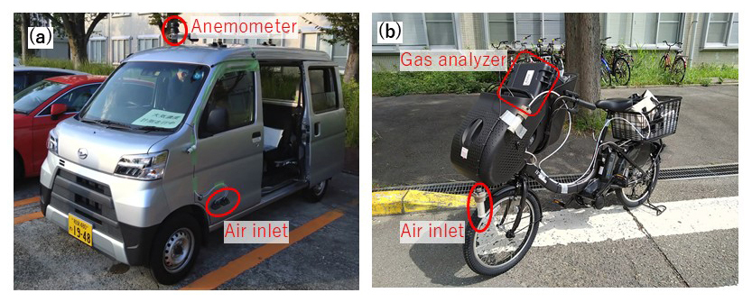
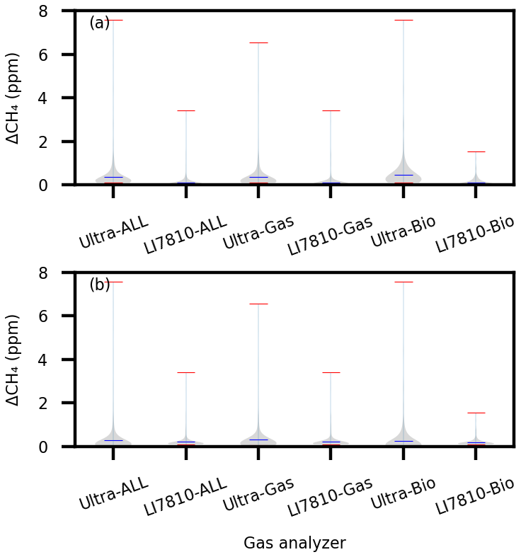
Figure A2 Violin plots for ΔCH₄ enhancements (ΔCH₄) measured at LIs based on the vehicle measurements by the Mira Ultra analyzer installed at 0.5 m above the ground and the LI-7810 analyzer at 1.85 m. Panel (a) is ΔCH₄ identified by the Ultra analyzer, and panel (b) is ΔCH₄ identified by the LI-7810 analyzer. The plots are summarized for natural gas and biogenic sources as well as for all LIs. The source attributions are based on C₂ : C₁ for the Ultra analyzer and ΔCH₄ for the LI-7810 analyzer.

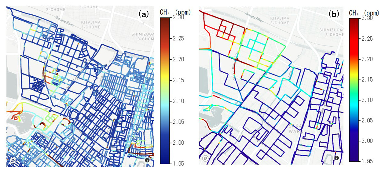
Figure A3 CH₄ concentrations based on the bicycle (a) and vehicle (b) measurements for Sakai Ward as an example of how intensively the bicycle measurements covered the streets compared with the vehicle measurements. To remove the daily variations in the CH₄ concentration for visualization, the CH₄ concentration was rescaled so that the 5th percentile of the CH₄ concentration on each measurement day was 2.0 ppm. Visualization was achieved using Plotly in Python, which uses © OpenStreetMap as a basemap provided by © mapbox.

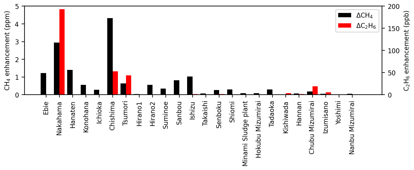
Figure A4 CH₄ and C₂H₆ enhancements within 500 m of a sewage treatment plant based on vehicle measurements. Note that the Minami sludge plant was the only sludge plant, and the others were sewage treatment plants or pump stations. The enhancements could be slightly biased, especially when the wind directions were not ideal, because the concentrations were measured on public roads, which hampered driving circles around all the sewage treatment plants.

Table A1 Date, travel distance, speed, and the type of the gas analyzer used in the campaign for the vehicle measurements.

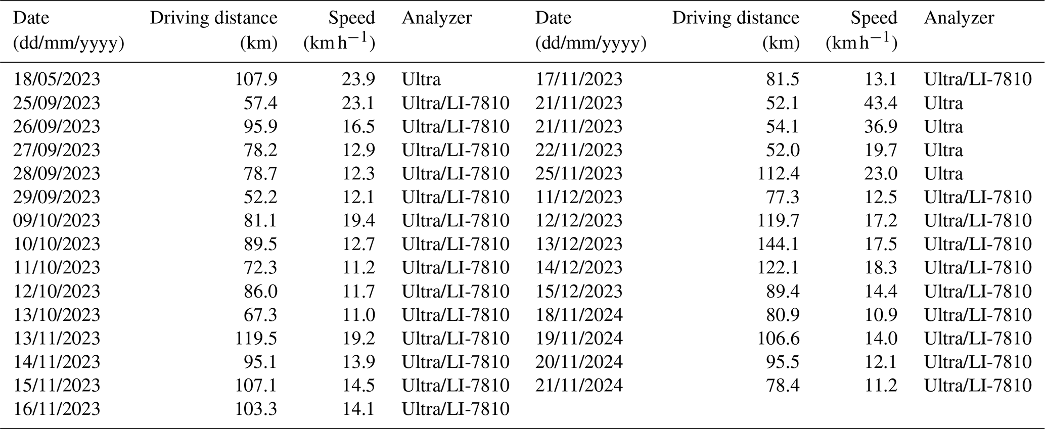
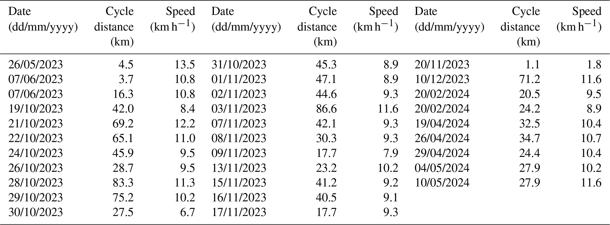
Table A2 Date, travel distance, and speed for the bicycle measurements.