Assessment of 16-year tropospheric ozone trends from the IASI Climate Data Record

Assessing tropospheric ozone (O₃) variability is essential for understanding its impact on air quality, health, and climate change. The Infrared (IR) Atmospheric Sounding Interferometer (IASI) mission onboard the Metop platforms has been providing global measurements of O₃ concentrations since 2007. This study presents the first comprehensive analysis of the 16-year O₃ Climate Data Record (CDR) from IASI/Metop (2008–2023), a homogeneous dataset offering valuable insights into the variability and long-term trends of tropospheric O₃. The IASI-CDR ozone product is evaluated against TROPESS (TRopospheric Ozone and its Precursors from Earth System Sounding) O₃ retrievals from the Cross-track Infrared Sounder (CrIS). The comparison shows excellent agreement for total ozone (biases <1.2 %, correlations >0.97) and good agreement for tropospheric ozone (biases 10 %–12 %, correlations 0.77–0.91). Comparisons with ozonesonde data indicate that IASI underestimates tropospheric ozone by 2 % in the tropics and by up to 10 % in mid and high latitudes. Drift analysis indicates the long-term temporal stability of IASI tropospheric ozone, with values below 3 % per decade globally and regionally, satisfying the stability criterion requirement. IASI data reveal a global decline in tropospheric O₃ (−0.08 ± 0.05 DU yr⁻¹, p=0.01), strongest in the tropics and Europe. The comparison with ozonesonde data, shows high-certainty decreases consistently observed in the tropics across all datasets (IASI, smoothed sonde, and raw sonde), supporting the robustness of the findings in this region. Vertical analysis reveals that negative trends dominate in the lower troposphere, while positive trends in the upper troposphere align with ultraviolet (UV) satellite observations. This vertical contrast highlights the importance of separating lower and upper tropospheric layers when comparing IR and UV datasets. Although discrepancies remain when considering the full tropospheric column, both UV and IR satellite instruments show a significant drop in tropospheric ozone starting in 2020, partly due to pandemic-related emission reductions. This study emphasizes the importance of long-term, consistent datasets for tracking ozone trends and the need for improved data retrieval and integration to address regional and temporal discrepancies.

1 Introduction

Tropospheric and stratospheric ozone (O₃) are key components of Earth's atmosphere with distinct roles and impacts. Stratospheric ozone plays a protective role by absorbing the majority of the Sun's harmful ultraviolet (UV) radiation, thus shielding life on Earth. The depletion of stratospheric ozone due to chlorofluorocarbons (CFCs) has led to global efforts like the Montreal Protocol, which has been essential in mitigating further losses (WMO, 2018). The interactions between the two layers are complex, as stratosphere-troposphere exchange processes influence tropospheric ozone levels and, subsequently, surface air quality (Neu et al., 2014; Ziemke et al., 2019; Thompson et al., 2021).

In contrast, tropospheric ozone is a secondary pollutant formed through photochemical reactions involving precursors such as nitrogen oxides (NO_x), volatile organic compounds (VOCs) and carbon monoxide (CO) in the presence of sunlight (Seinfeld and Pandis, 1998). It is a short-lived climate forcer and a major contributor to air pollution, affecting human health by aggravating respiratory and cardiovascular conditions, and reducing crop yields and ecosystem productivity (Fleming et al., 2018; Mills et al., 2018; Tai et al., 2014; Murray et al., 2024). Furthermore, both tropospheric and stratospheric ozone play a significant role in radiative forcing, with tropospheric ozone having particularly pronounced effects in tropical and subtropical regions (Worden et al., 2008; Bowman and Henze, 2012; Gaudel et al., 2018). By absorbing infrared radiation, it also contributes to global warming, acting as a potent greenhouse (IPCC, 2021). Understanding its sources and dynamics is essential for developing effective mitigation strategies to address its environmental and health impacts.

Recent studies have significantly advanced our understanding of tropospheric ozone trends, particularly those derived from satellite data, emphasizing the complexity and variability of ozone concentrations across different regions and time scales. These trends are influenced by both natural and anthropogenic factors (Lelieveld et al., 2008; Wespes et al., 2017; Tarasick et al., 2019; Ziemke et al., 2019). For example, the first phase of the Tropospheric Ozone Assessment Report (TOAR-I) highlighted that free tropospheric ozone has increased since the industrial era and continued to rise in recent decades (Gaudel et al., 2018; Tarasick et al., 2019; Gulev et al., 2021). Regional trends are more varied: while ozone levels have decreased in summer in North America and Europe, they have increased in Asia (Gaudel et al., 2018, 2020; Wespes et al., 2018). Several studies based on in situ measurements have observed similar patterns. Stauffer et al. (2024) analyzed 25 years of ozone profiles over equatorial Southeast Asia, observing increases in free tropospheric ozone (5 %–15 % per decade), which they attributed to reduced convection between February and April, suppressing ozone dilution and promoting the accumulation of biomass burning emissions. Likewise, Wang et al. (2022) reported rising global ozone levels, especially in the free troposphere, from 1980 to 2017 using IAGOS data. In both cases, limitations in spatial sampling have to be considered (Miyazaki and Bowman, 2017).

The COVID-19 pandemic in 2020 marked a significant turning point in tropospheric ozone trends. Studies indicate that reduced emissions of ozone precursors during the economic slowdown of 2020 led to declines in ozone levels (Miyazaki et al., 2020; Ziemke et al., 2021). Satellite-based observations suggest that the increase of the tropospheric ozone burden ended in 2020, with no increase observed between 2021 and 2023 (Dunn et al., 2024). This stagnation coincided with negative ozone anomalies in the free troposphere in the Northern Hemisphere (NH) in 2020, as documented by ozonesonde, lidar and commercial aircraft data (e.g. Steinbrecht et al., 2021; Chang et al., 2022, 2023a). Over Europe, satellite observations from GOME-2 and IASI revealed a substantial 11 %–15 % decrease in lower tropospheric ozone during 2020–2022, with the largest reduction occurring in 2022, suggesting that both pandemic-related emission reductions and additional regional drivers played a role (Pimlott et al., 2024). Model simulations attribute these decreases to reduced emissions of ozone precursors, with levels comparable to those of the mid-1990s (Miyazaki et al., 2020; Steinbrecht et al., 2021).

Despite these advancements, reconciling trends derived from satellite data remains challenging due to discrepancies between UV and infrared (IR) satellite sounders (Gaudel et al., 2018). UV sounders generally report positive trends (e.g., Cooper et al., 2014; Ziemke et al., 2019; Liu et al., 2022; Fadnavis et al., 2025; Gaudel et al., 2024), while IR sounders often indicate negative trends (Wespes et al., 2018; Dufour et al., 2018, 2025). However, more recent studies have begun to bridge these differences. For instance, Pope et al. (2024) identified weak negative trends with significant uncertainties in lower tropospheric ozone over North America, Europe, and East Asia from 2008 to 2017 using both UV and IR data. Similarly, Pimlott et al. (2024) reported small negative trends in European lower tropospheric ozone during the same period based on UV satellite observations. A longer-term satellite analysis (1996–2017) by Pope et al. (2024) confirmed significant increases in lower tropospheric ozone across tropical and subtropical regions, consistent with trends in total tropospheric ozone, underscoring continued challenges in constraining long-term variability. Complementary ground-based records also reveal nuanced trends, with recent TOAR-II datasets showing increasing ozone over most of Asia, mixed patterns in Europe and North America, and smaller post-COVID trends (Van Malderen et al., 2025a, b). These findings underscore the variability of trends depending on the temporal period and highlight the importance of harmonizing and validating satellite observations to improve the reliability of ozone trend analyses.

Further investigation is needed to enhance our understanding of tropospheric ozone variability, improve knowledge of ozone trends, and ensure consistent long-term monitoring. The Infrared Atmospheric Sounding Interferometer (IASI) instruments onboard the Metop satellites provide a consistent dataset since 2007, enabling long-term ozone monitoring. This study, conducted within the framework of the TOAR-II project, analyzes the IASI O₃ Climate Data Record (IASI-CDR), recently processed by EUMETSAT under the auspices of the Atmospheric Composition Monitoring Satellite Application Facility (AC SAF) project, offering a homogeneous 16-year dataset (2008–2023) for the first time. The primary objectives are (1) to assess the quality and consistency of the IASI-CDR O₃ product, and (2) to investigate the spatiotemporal variability and long-term ozone trends. This work aims to deepen our understanding of ozone dynamics and its evolution over time. Section 2 describes the datasets and the methods used in this study, Sect. 3 presents the validation results of the IASI-CDR O₃ product using independent measurements, Sect. 4 gives a comprehensive analysis of tropospheric ozone trend estimates, and Sect. 5 summarizes the main findings of this study.

2 Data and methods

2.1 Data

2.1.1 The IASI-CDR O₃ product

The IASI instruments, named IASI-A, IASI-B, and IASI-C, are carried aboard the Metop-A, Metop-B, and Metop-C satellites, launched in 2006, 2012, and 2018, respectively (Clerbaux et al., 2009). Metop-A entered orbital drift in 2017 and stopped providing IASI data in October 2021. The IASI instruments provide data twice daily with overpass times at approximately 09:30 AM and 09:30 PM local solar time, and spatial resolution of 12 km diameter at nadir. The instrument has a spectral resolution of 0.5 cm⁻¹ (after apodization) over the 645–2760 cm⁻¹ range and a radiometric resolution of 0.25 K for temperature at 280 K (Hilton et al., 2012), ensuring high precision for atmospheric composition monitoring.

This study uses O₃ Level 2 products (vertical profiles) retrieved with the Fast Optimal Retrievals on Layers for IASI (FORLI) software, version v20151001, developed by ULB and LATMOS (Hurtmans et al., 2012). This dataset will hereafter be referred to as IASI-FORLI. FORLI processes IASI Level 1C radiances together with meteorological Level 2 data to retrieve ozone profiles using an optimal estimation method. This approach combines measured infrared radiances with a priori ozone information to constrain the solution. The a priori profile provides an initial estimate of the atmospheric state and helps stabilize the retrieval in poorly constrained layers, especially when the measurements alone are not sufficient. In FORLI, a single a priori profile is used, based on the global mean McPeters/Labow/Logan climatology (McPeters et al., 2007), along with its associated variance-covariance matrix. The vertical sensitivity of the retrieval is described by the averaging kernels (AKs), which indicate how much the retrieved profile depends on the measurements versus the a priori. The degrees of freedom for signal (DOFs) quantify the amount of independent information extracted from the observations. Variations in the choice of a priori, the shape of AKs, or DOFs values can directly influence the retrieval accuracy and vertical resolution, especially in regions where IASI sensitivity is limited. The FORLI software is fully described in Hurtmans et al. (2012).

The IASI-FORLI O₃ product has been widely used in numerous studies such as urban pollution (Ancellet et al., 2024), ozone hole monitoring (Scannell et al., 2012; Gazeaux et al., 2013; Safieddine et al., 2020), interannual variability (Safieddine et al., 2013, 2014, 2016; Wespes et al., 2016, 2017) and long-term trend analyses (Gaudel et al., 2018; Wespes et al., 2018; Pope et al., 2024). It has also been extensively validated (Dufour et al., 2012; Pommier et al., 2012; Boynard et al., 2016, 2018; Keppens et al., 2018). In particular, Boynard et al. (2018) validated the latest version of IASI-FORLI v20151001 O₃ product for the period over 2008–2017, reporting a global mean difference of less than 2 % in the total ozone column (TOC) compared to independent measurements such as GOME-2, with larger discrepancies observed at high latitudes. For the tropospheric ozone column, they found a positive bias of 4 %–5 % at high latitudes and a negative bias of 11 %–19 % in midlatitudes and the tropics.

A few years ago, the FORLI v20151001 version was implemented in the EUMETSAT near real time (NRT) processing facility in the framework of the AC SAF project. Since 4 December 2019, the IASI-FORLI O₃ product has been operationally distributed to users through the EUMETCast system and made available to users on the AERIS website (https://iasi.aeris-data.fr/O3/, last access: 11 July 2025). The IASI-FORLI O₃ Level 2 and Level 3 products are included in the European Space Agency Ozone Climate Change Initiative (Ozone_cci, http://www.esa-ozone-cci.org, last access: 11 July 2025) and the European Centre for Medium Range Weather Forecasts (ECMWF) Copernicus Climate Change (C3S, https://cds.climate.copernicus.eu/, last access: 11 July 2025) projects, respectively. These initiatives aim to develop comprehensive O₃ datasets that are relevant for climate monitoring, specifically as essential climate variables (ECVs). However, the IASI-FORLI dataset is not consistent, as it was processed based on different versions of the IASI Level 1C (radiances) and Level 2 (temperature, humidity and cloud) Product Processing Facility (PPF) between 2007 and 2019, as summarized in Tables 1 and 2 of Bouillon et al. (2020). Consequently, it should be used with caution for long-term trend studies, as these differences have been shown to introduce a “jump” leading to an “artificial drift” in the tropospheric ozone time series, particularly around the end of 2010 (Boynard et al., 2018).

In this context, EUMETSAT on behalf of AC SAF has reprocessed the IASI-FORLI v20151001 product using the reprocessed IASI Level 1C radiances (EUMETSAT, 2018) and Level 2 temperature and humidity products (EUMETSAT, 2022), to ensure consistency and homogeneity throughout the entire IASI period. This process resulted in the creation of a homogeneous IASI O₃ product: the IASI-CDR O₃ product (AC SAF, 2025). To account for potential biases arising from the orbital drift of Metop-A, only IASI-A data up to December 2019 are included in the CDR. From that point onwards, the record seamlessly continues using IASI-B data, as the two instruments are identical (Boynard et al., 2018; Bouillon et al., 2020). Data from IASI-C, which is the same instrument as IASI-A and IASI-B, are not reprocessed into the CDR, but are produced using the same version of EUMETSAT Level 1C and 2 PPF and FORLI algorithm (v20151001) as the CDR, ensuring consistency and forming the Interim CDR (ICDR) component. Henceforth, we refer to two IASI products: the inhomogeneous IASI-FORLI product and the homogeneous IASI-CDR product. The latter includes the reprocessed CDR from IASI-A and IASI-B (2008–2023), as well as the ICDR from IASI-C (2020–2023). Due to computing time constraints, only approximately 3.5 out of 10 IASI pixels were processed throughout the entire IASI-CDR time series.

This dataset provides vertical ozone profiles as partial columns distributed across 40 atmospheric layers (from the surface to 40 km altitude), along with a separate column for the upper atmosphere above 40 km. Each retrieval includes quality metrics such as a priori profiles, total error estimates, averaging kernel (AK) matrices, and quality flags. To ensure data quality, only retrievals associated with a general quality flag (GQF) equal to 1 are used. This GQF includes a cloud flag to filter out cloud-contaminated scenes, allowing retrievals to be performed only on clear or mostly clear scenes with fractional cloud cover below 13 %, as identified using cloud information from the EUMETSAT operational processing (August et al., 2012). It is also recommended to exclude data associated with low degrees of freedom for the signal (DOFS <2), a limitation often affecting data from polar regions like Antarctica (Boynard et al., 2018). In this study, we analyze both total and tropospheric ozone columns. For the tropospheric column, we use the column integrated from the surface to the thermal tropopause, as defined by the World Meteorological Organization (WMO) (World Meteorological Organization, 1957). The thermal tropopause is calculated from the IASI L2 temperature profiles. As highlighted by Elshorbany et al. (2024), relying on a fixed pressure level for the tropopause may lead to inaccuracies due to temporal variations in the thermal tropopause height, which justifies the use of the thermal tropopause in this analysis.

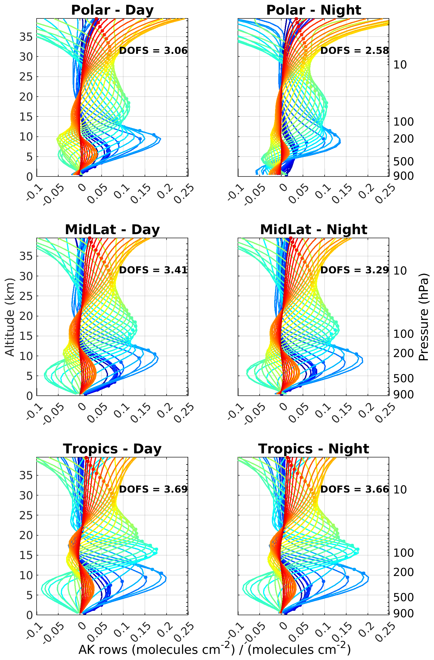
Figure 1 Illustration of IASI-B averaging kernels (AK) averaged across three latitude bands (polar regions, midlatitudes and tropics) for 7 July 2023 (separated into day and night conditions), showing the distribution of information in the vertical ozone profile. Each line represents a row of the AK matrix, and the circles indicate the altitude of each kernel. The polar regions, midlatitudes and tropics correspond to the following bands: 60–90° North and South, 30–60° North and South, and 30° S–30° N, respectively.

Table 1 IASI/Metop-B retrieval errors, including smoothing and measurement errors, along with the DOFS for total and tropospheric columns, averaged on 15 of each month for both daytime and nighttime across 30° latitude bands in 2023.

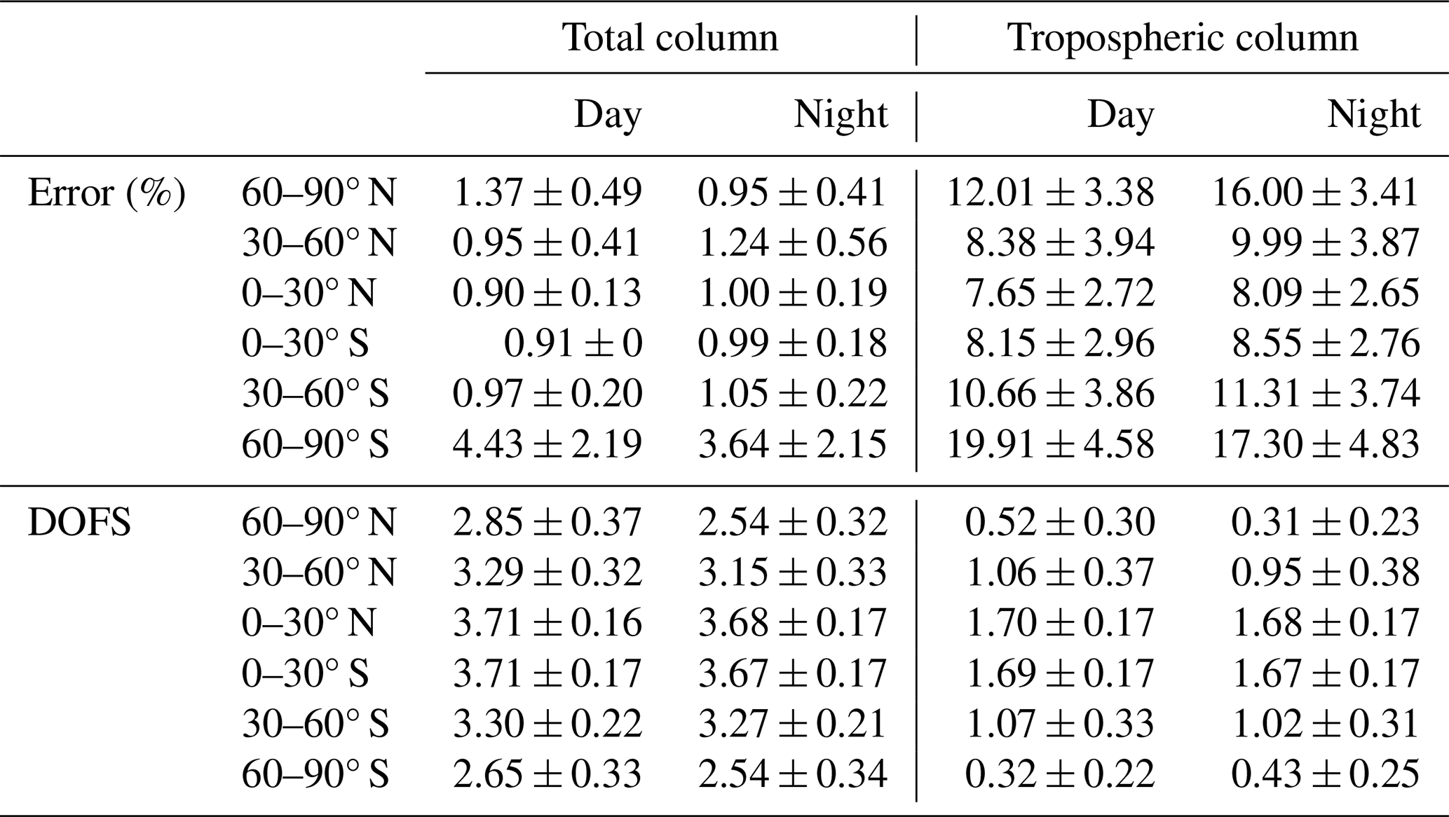
Figure 1 shows the vertical sensitivity of IASI in the polar, midlatitude, and tropical regions, separated into day and night conditions. In all regions, the averaging kernel (AK) values do not reach their maximum at the nominal altitudes, indicating that the ozone retrieval at each level is impacted by contributions from other altitudes. The maximum sensitivity is observed around 8 km, regardless of day or night conditions. For the midlatitude and tropical regions, there are no significant differences between day and night sensitivity. However, at high latitudes, the sensitivity in the lower troposphere is notably weaker at night, as shown by both the averaging kernel curves and the DOFS values (DOFS of ∼ 3 during the day and ∼ 2.5 at night). The tropical regions, benefiting from higher temperatures, show the highest sensitivity, with DOFS values of ∼ 3.7.

The variability in data sensitivity and quality is reflected in both the error and DOFS analyses, revealing differences across latitude bands and between day and night (see Table 1). In high latitude regions (60–90° N and 60–90° S), total column errors are significantly higher, particularly in the Southern Hemisphere (SH), where daytime errors reach 4.43 % compared to 3.64 % at night. Similarly, in the NH, daytime errors (∼ 1.37 %) are higher than nighttime errors (∼ 0.95 %). Tropospheric column errors are even more pronounced in these regions, especially in the SH, where daytime errors peak at ∼ 19.91 %. These results highlight reduced data quality and sensitivity in polar regions, particularly at night, due to lower surface temperatures and weaker signals. In the midlatitudes (30–60° N and 30–60° S), total column errors are relatively low and consistent between day and night, ranging from ∼ 0.95 % to ∼ 1.24 %. In the tropics (0–30° N and 0–30° S), total column errors are even lower, ranging from ∼ 0.90 % to ∼ 1.00 %. Tropospheric column errors in these regions are similarly low, with slightly higher values in the SH midlatitudes, suggesting generally higher data quality. Tropical regions benefit from more favorable atmospheric conditions and higher temperatures, which contribute to significantly better data quality compared to the polar regions.

The DOFS analysis provides further insights into data sensitivity. In high-latitude regions, the DOFS values for the total column decrease at night (e.g., ∼ 2.85 during the day vs. ∼ 2.54 at night in the NH). Tropospheric DOFS values are particularly low in the SH (∼ 0.32 during the day and ∼ 0.43 at night), reflecting limited sensitivity and reduced information content in polar regions. In the midlatitudes, total column DOFS values are higher but show a slight decrease from day to night (e.g., ∼ 3.29 during the day vs. ∼ 3.15 at night in the NH). Tropospheric DOFS remain around ∼ 1.0, indicating moderate sensitivity. In the tropics, DOFS values are the highest for both the total and tropospheric columns. Total column DOFS remain consistent between day and night (∼ 3.7), while tropospheric DOFS are around ∼ 1.7, reflecting enhanced sensitivity and information content in these regions.

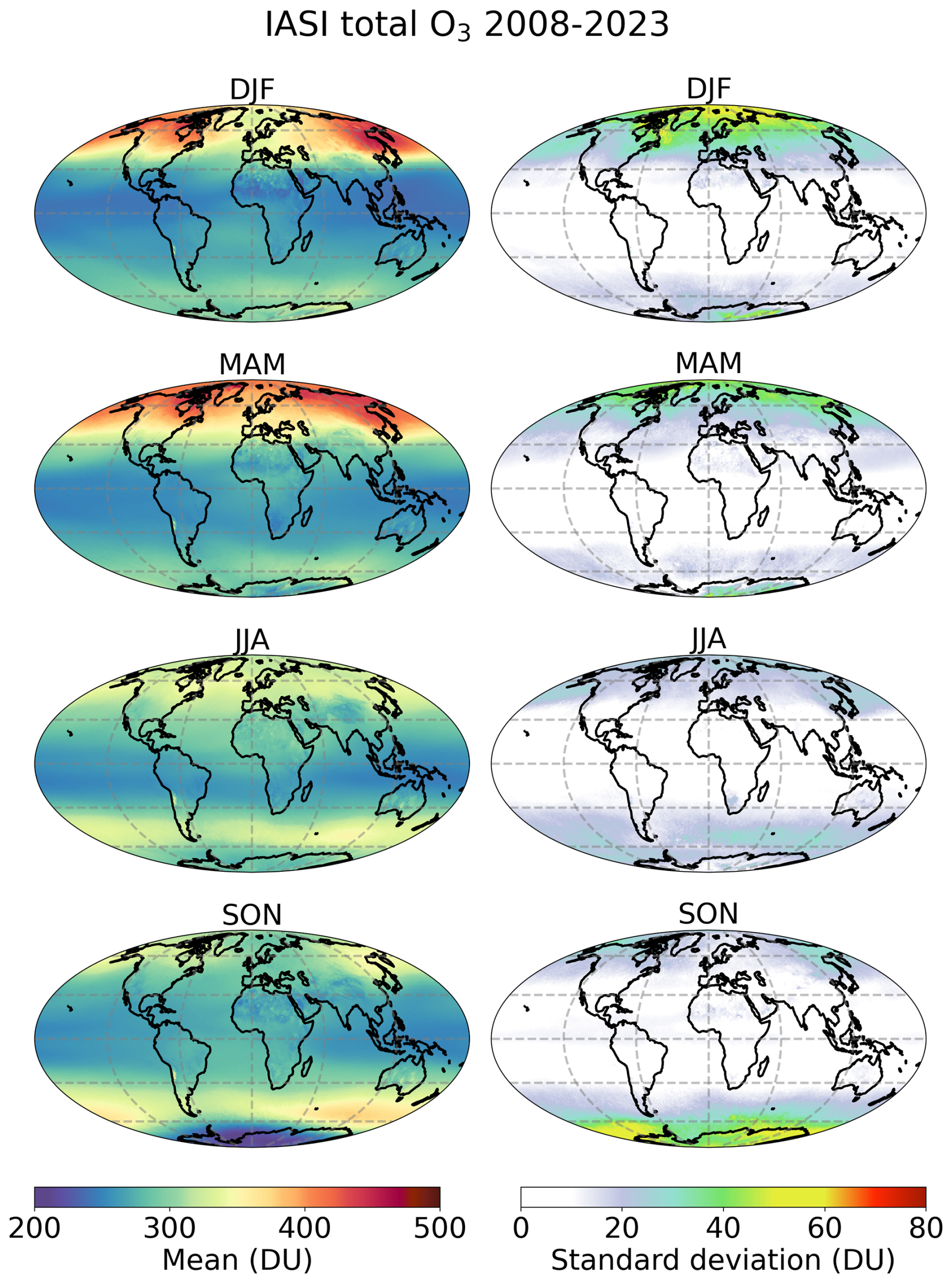
Figure 2 Spatial and seasonal distribution of total ozone column derived from IASI-CDR over the period 2008–2023 in Dobson units (DU): mean (left) and standard deviation (right). DJF, MAM, JJA and SON represent December–January–February, March–April–May, June–July–August and September–October–November, respectively. The data are averaged onto a global 1°×1° grid.

In summary, the tropics demonstrate the highest data quality and sensitivity, while the polar regions, particularly at night, show reduced sensitivity and increased uncertainty, especially in the tropospheric column. This pattern reflects the influence of atmospheric conditions and instrument performance across regions and times.

To analyze tropospheric ozone, it is essential to first validate the total ozone column, followed by the tropospheric ozone column. In the following, we describe both the total and tropospheric columns, which will be validated in Sect. 3.

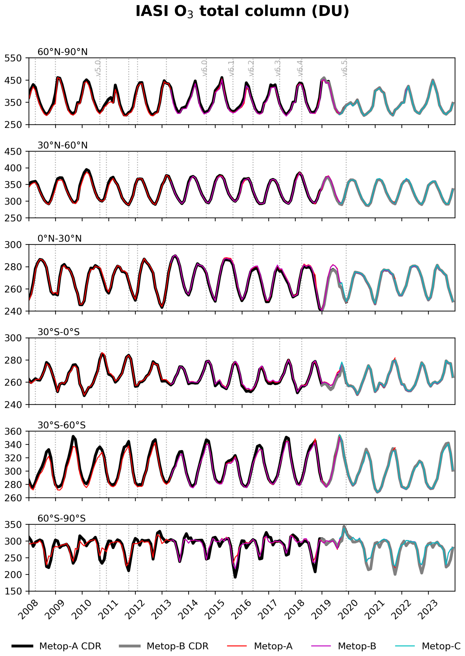
Figure 3 Monthly time series of IASI total ozone column derived from the CDR products in Dobson units (DU) for Metop-A and Metop-B (in black and gray) over six 30° latitude bands. The time series of IASI-FORLI v20151001 product (Boynard et al., 2018) is also shown for the three Metop (in red, magenta and cyan). Note that the y−scale differs between the latitude bands. The vertical lines represent the date of the EUMETSAT L2 Product Processing Facility version changes (see Bouillon et al., 2020 for further details on these changes).

Figure 2, which illustrates the spatial and seasonal variability of total ozone from the IASI-CDR product, shows a pronounced latitudinal gradient. Ozone concentrations are lower in the tropics, where the ozone layer is thinner, and increase toward higher latitudes. This pattern can be observed each year, as shown in Fig. 3 illustrating the monthly time series of the IASI O₃ total columns between 2008 and 2023. This is primarily driven by two factors: significant ozone production in the tropics due to intense solar UV radiation and the Brewer-Dobson circulation, which transports ozone from the tropics to the poles, leading to an accumulation at middle and high latitudes (Dessler, 2000; Wespes et al., 2018). Seasonal variations also play a role. At high latitudes, ozone levels are lowest in winter due to the polar night and the isolation of ozone-poor air by the polar vortex, while levels increase in spring and early summer as sunlight returns. However, polar regions face to lower levels in late summer due to photochemical destruction. We clearly see very low levels of total ozone in Antarctic, where photochemical reactions during the austral spring cause the ozone hole (WMO, 2018). Figure 3 also highlights key events, such as the largest ozone hole in 2015 (associated with El Niño), the smallest ozone hole in 2019 (linked to a sudden stratospheric warming; Safieddine et al., 2020) over Antarctica, and a smaller ozone hole in 2020 over the North Pole. At midlatitudes, total ozone peaks in spring when ozone is transported from the tropics and decreases in summer due to photochemical loss, with lower levels in fall and winter. In contrast, the tropics have relatively stable ozone levels throughout the year, as sunlight and ozone transport remain relatively stable. Another important insight provided in Fig. 3 is the comparison of the total ozone columns across the three IASI instruments and two IASI products (IASI-CDR and IASI-FORLI). This will be discussed hereafter.

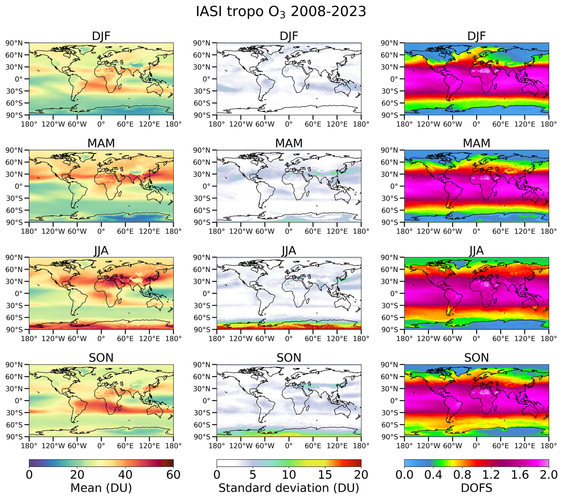
Figure 4 Same as Fig. 2, but for the tropospheric ozone column. The DOFS associated with the tropospheric column is also shown (right panels). The tropospheric column is integrated from the surface to the thermal tropopause, as defined by the World Meteorological Organization (WMO, 1957).

Figure 4 (left panels) illustrates the spatial and seasonal variability of tropospheric ozone from the IASI-CDR product. Tropical regions have lower ozone levels due to humid conditions and active convection, with localized plumes during biomass burning seasons. The midlatitudes experience higher concentrations in spring and summer, driven by photochemical production from anthropogenic emissions of precursors like NO_x and VOCs, particularly over densely populated areas of China and northern India (Logan, 1985; Fusco and Logan, 2003; Safieddine et al., 2013; Wespes et al., 2016). Long-range transport, such as ozone from Asia to the Pacific, also contributes to variability (Zhang et al., 2008). In the eastern Mediterranean Basin, summer ozone levels are linked to stratosphere-troposphere exchange (Safieddine et al., 2014). Significant fire activity around 20–40° S in spring also affects seasonal distributions (Wespes et al., 2017). High latitudes have lower background levels due to minimal emissions and reduced photochemistry, although enhancements occur in spring, influenced by transport and stratosphere-troposphere exchange, with additional summer increases in the Arctic (Stohl et al., 2003). Winter months show reduced photochemical activity across all regions due to lower sunlight. These patterns are observed annually, as shown in Fig. 5, which illustrates the monthly time series of tropospheric ozone from the IASI-CDR product.

As shown in Fig. 4 (middle panels), the standard deviation for tropospheric ozone is larger in polar region, which is due to the lower IASI sensitivity in those regions because of low temperature. The larger standard deviation observed during the June–July–August (JJA) season over Antarctica is partly due to the complexities involved in accurately defining the tropopause altitude in this region. Unlike other areas, Antarctica can exhibit two distinct tropopauses within the temperature profile, making the conventional temperature-based definition of the tropopause unreliable. This phenomenon complicates the identification of a single tropopause, which can lead to discrepancies in understanding the distribution of ozone and the exchange between the troposphere and stratosphere. The use of temperature profiles to estimate tropopause height is thus not suitable for the South Pole, where alternative dynamic or chemical criteria are more appropriate for defining the tropopause structure (Zängl and Hoinka, 2001; Xian and Homeyer, 2019).

The DOFS associated with the tropospheric ozone column, shown in Fig. 4 (right panels), exhibit a clear meridional gradient, with higher values in the tropics and lower values in the polar regions. This gradient is driven by the temperature-dependent IASI sensitivity, which influences the amount of information that can be retrieved across different latitudes. In the tropics, elevated temperatures enhance IASI sensitivity, resulting in consistently high DOFS values near 2.0 across all seasons, indicating that two independent pieces of information can be reliably retrieved. In contrast, midlatitude regions show more variability in DOFS, typically ranging from 1.0 to 1.5, due to more fluctuating temperatures. Polar regions, where IASI sensitivity is reduced due to colder temperatures, generally exhibit lower DOFS values, often falling below 1.0. The seasonal patterns further emphasize these differences: the tropics maintain consistent DOFS values year-round, while midlatitudes experience greater fluctuations, particularly during transitional seasons like spring and fall.

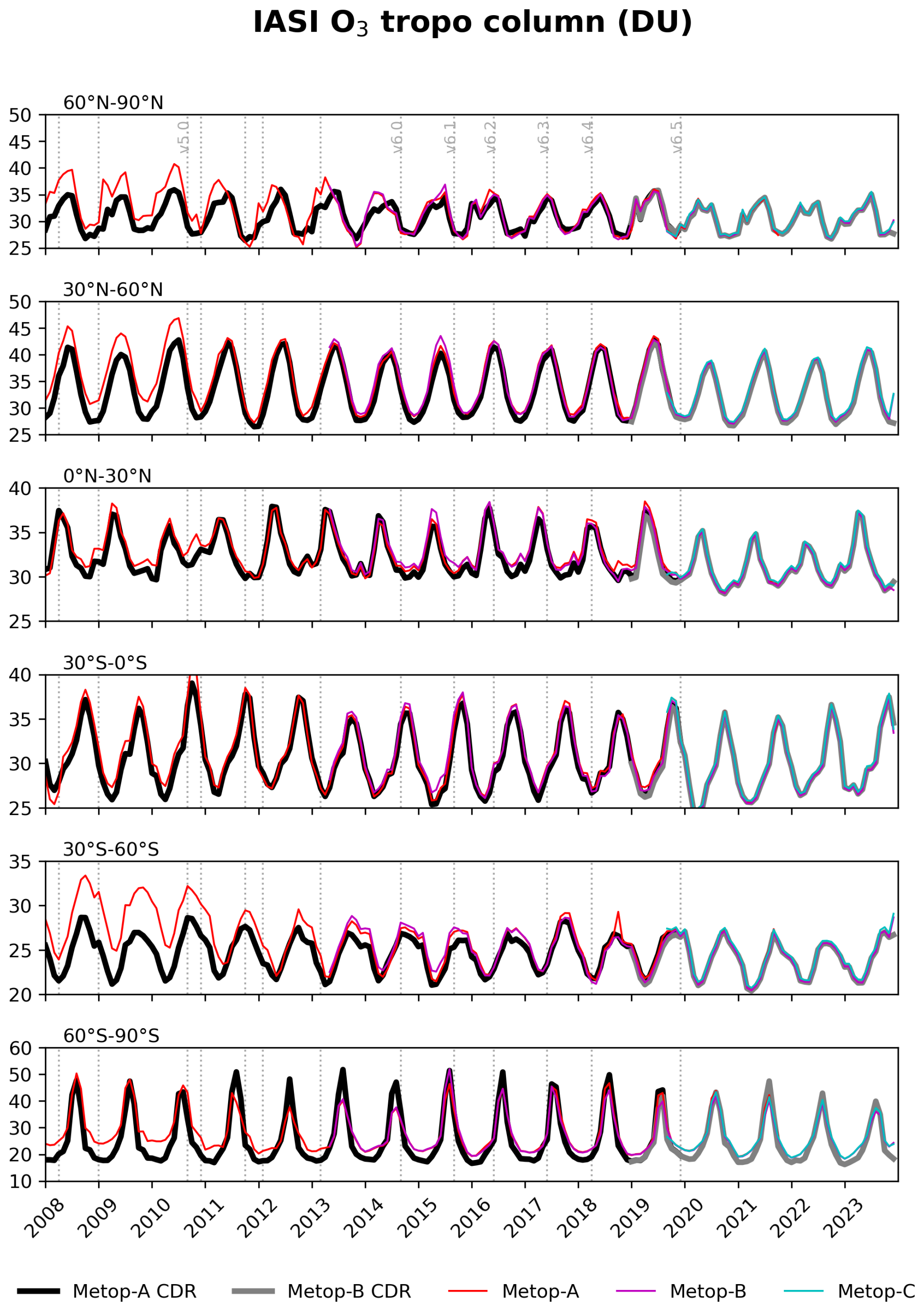
Figure 5 Same as Fig. 3, but for the tropospheric column. The tropospheric column is integrated from the surface to the thermal tropopause, as defined by the World Meteorological Organization (WMO, 1957).

Figures 3 and 5 compare the monthly total and tropospheric ozone time series, respectively, between the three IASI instruments with both IASI-CDR and IASI-FORLI products. A strong consistency is found among the three IASI instruments, with a global bias of less than 0.05 % for the total column and less than 1 % for the tropospheric column. This consistency is observed between IASI-B and -C from 2020 to 2023, and between IASI-A and -B for 2019, as these are the only overlapping periods for these instrument pairs in the IASI-CDR product. For the total column (see Fig. 3), there is a strong agreement between IASI-CDR and IASI-FORLI for Metop-A and -B, which suggests that the total column product is not impacted by the different changes in Eumetsat L2 PPF. However, for the tropospheric column (see Fig. 5), large differences between the two products are observed until end of 2010, corresponding to a change in the Eumetsat Level 2 PPF version. These discrepancies in the tropospheric column before 2010 are likely due to uncertainties in the tropopause height, as the IASI-FORLI product used an earlier version of the temperature profiles to determine the thermal tropopause, in contrast to the more recent version used by IASI-CDR. This is further supported by the fact that we do not observe the same pattern in the differences for the total column product, suggesting that the variations in the tropospheric column are linked to the differing temperature profiles used by the two products. After this period, agreement improves notably across all latitude bands although discrepancies remain visible especially in the high latitudes and southern midlatitudes. Our analysis of the monthly ozone time series shows that IASI-CDR and IASI-FORLI converge starting from late 2019, as expected, since the same version of Eumetsat L2 PPF was used for both products.

2.1.2 The TROPESS-CrIS O₃ product

The Cross-track Infrared Sounder (CrIS) is an infrared Fourier transform spectrometer on board the NOAA Suomi- National Polar-orbiting Partnership (Suomi-NPP) and the Joint Polar Satellite System1 (JPSS-1 or NOAA-20) satellite operating since 2011 and 2017, respectively (https://www.star.nesdis.noaa.gov/jpss/CrIS.php, last access: 11 July 2025) (Luo et al., 2024a). CrIS measures radiances at over 1300 channels with a spectral resolution of 0.625 cm⁻¹ in three spectral bands – long-wave infrared (650–1095 cm⁻¹), mid-wave infrared (MWIR) (1210–1750 cm⁻¹), and short-wave infrared (2155–2550 cm⁻¹). It achieves near-global coverage twice daily with overpass times at approximately 01:30 AM and 01:30 PM local solar time, different from that of IASI/Metop. Each CrIS pixel or field of view (FOV) is circular with a 14 km radius at nadir (Luo et al., 2024a; Malina et al., 2024).

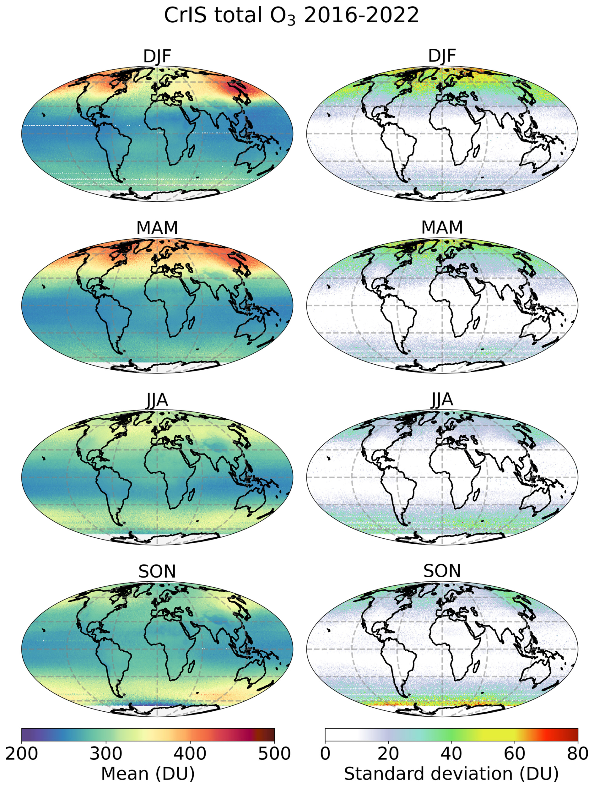
Figure 6 Spatial and seasonal distribution of total ozone column derived from CrIS data over the period 2016–2022 in Dobson units (DU): mean (left) and standard deviation (right). DJF, MAM, JJA and SON represent December–January–February, March–April–May, June–July–August and September–October–November, respectively. The data are averaged onto a global 1°×1° grid.

We use the TROPESS (TRopospheric Ozone and its Precursors from Earth System Sounding) CrIS ozone reanalysis stream summary product (TROPESS-CrIS, 2023), which contains vertically resolved concentrations of atmospheric O₃. Leveraging the MUlti-SpEctra, MUlti-SpEcies, Multi-Sensors (MUSES) algorithm (Fu et al., 2016), derived from the heritage of Aura/TES, TROPESS provides global datasets for the time period from December 2015 to December 2022. In late March 2019, an anomaly in the MWIR band caused a data gap from April to July 2019, which may affect trend analyses. After the instrument was fully restored, the data from early and late 2019 showed strong consistency (Iturbide-Sanchez et al., 2022). TROPESS uses an optimal estimation retrieval approach (Rodgers, 2000), building on the level-2 processing framework developed for Aura/TES (Tropospheric Emission Spectrometer) by Bowman et al. (2006). The MUSES algorithm retrieves atmospheric temperature, water vapor, and other trace gases simultaneously with ozone in the presence of clouds. The data are reported at 26 vertical levels from the surface to 0.1 hPa. TROPESS-CrIS O₃ products have been used in previous scientific studies; for example, tropospheric ozone changes during the COVID-19 lockdown have been assessed using CrIS data (Miyazaki et al., 2021); ozone retrieval improvement has been assessed by combining measurements from CrIS and from the TROPOspheric Monitoring Instrument (TROPOMI) aboard the Copernicus Sentinel-5 Precursor (S-5P) satellite (Malina et al., 2024). Pennington et al. (2025) compared the TROPESS-CrIS O₃ products with ozonesonde data and found a stable evolution of global tropospheric ozone bias of 0.21 ± 3.6 % decade⁻¹ for the period 2016–2021.

In this study we analyze the TROPESS-CrIS O₃ product over the period from January 2016 till December 2022. The data are averaged daily on a global grid with a resolution of 1°×1°. Figures 6 and 7 illustrate the spatial and seasonal distribution of CrIS O₃ total and tropospheric column, respectively, over the period 2016–2022. The spatial and season patterns between IASI and CrIS data are in very good agreement for both columns. A detailed comparison of these datasets is conducted in Sect. 3.

Table 2 List of the 43 sounding stations used for the validation exercise, including station name, geographical coordinates (latitude and longitude in degrees), period of observation, average number of measurements per month, and data source. Most data used in this study are sourced from HEGIFTOM (Harmonization and Evaluation of Ground-based Instruments for Free-Tropospheric Ozone Measurements). Incomplete HEGIFTOM time series have been supplemented with additional profiles from WOUDC, NOAA, or SHADOZ, and are labeled as HEGIFTOM/WOUDC, HEGIFTOM/NOAA, or HEGIFTOM/SHADOZ, respectively. HEGIFTOM time series originating from SHADOZ were directly copied from the original SHADOZ archive and are therefore identical to the original records. Data labeled “WOUDC” originate directly from the WOUDC archive and were not part of HEGIFTOM. Stations highlighted in bold are used for trend analysis.

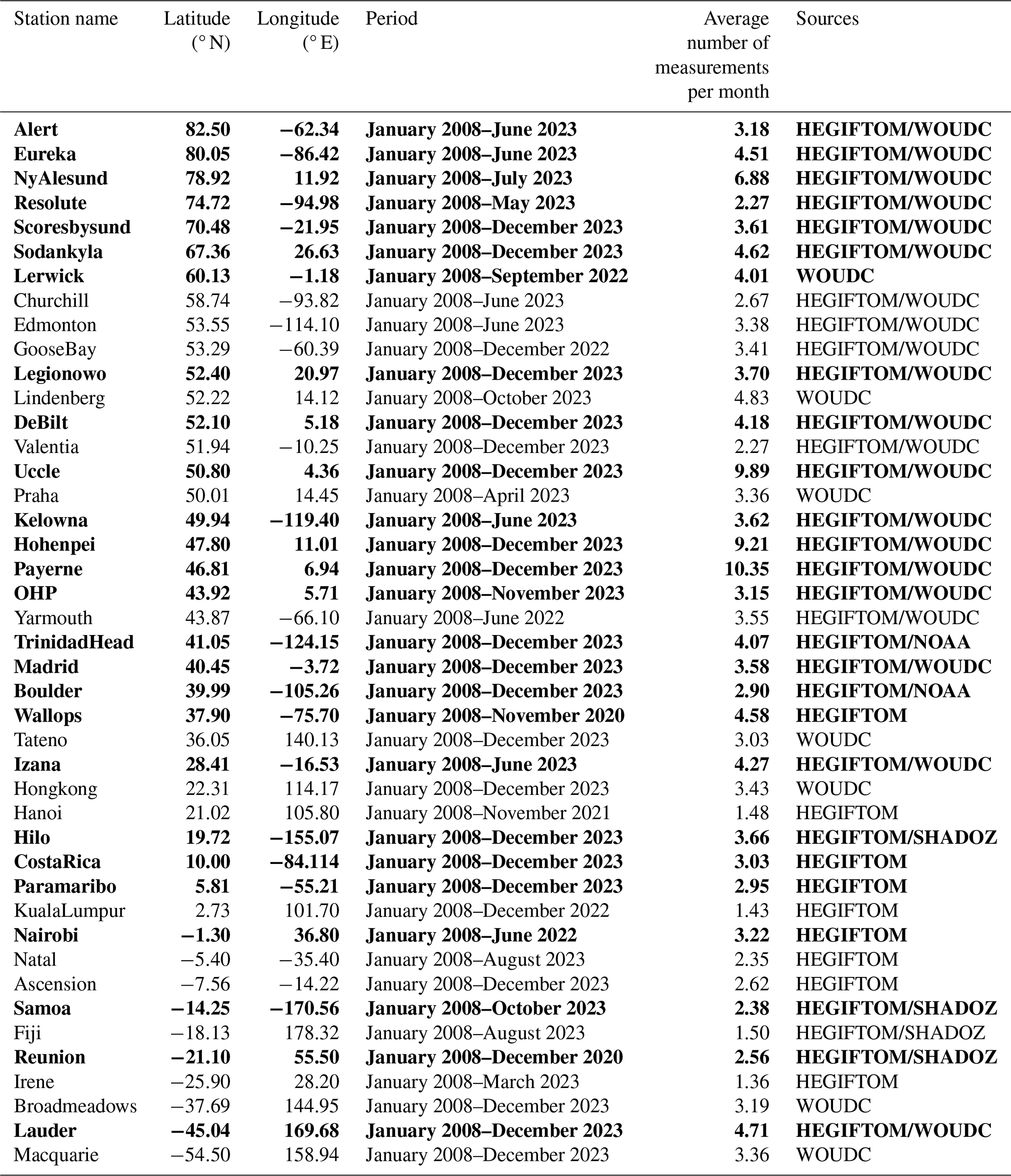
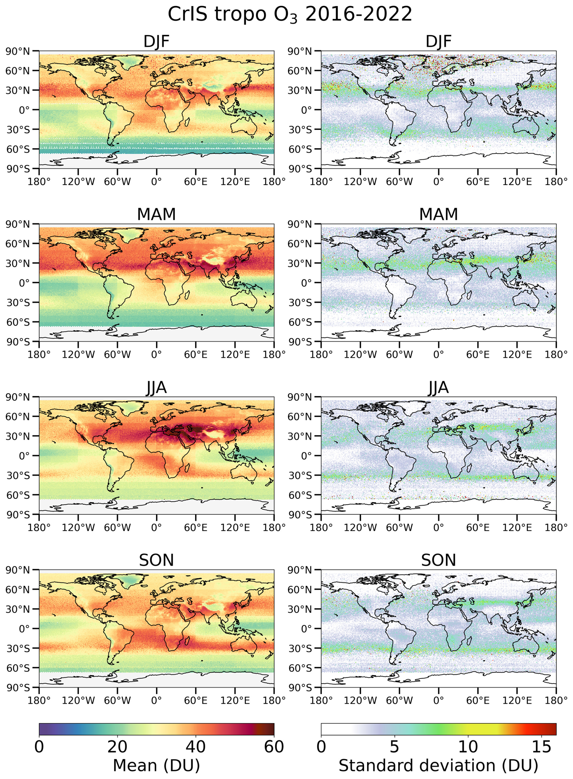
Figure 7 Same as Fig. 6, but for the tropospheric ozone column.

2.1.3 Ozonesonde data

We use ozonesonde data from the TOAR-II project, as part of the Harmonization and Evaluation of Ground-based Instruments for Free-Tropospheric Ozone Measurements (HEGIFTOM) working group (HEGIFTOM, 2025), which have been corrected for possible biases related to instrumental or processing changes (Van Malderen et al., 2025a). The incomplete HEGIFTOM sonde time series are supplemented with data from the World Ozone and Ultraviolet Radiation Data Centre (WMO/GAW Ozone Monitoring Community, 2025). Additional ozonesonde data were acquired from NOAA (NOAA, 2025), the Southern Hemisphere Additional Ozonesondes (SHADOZ, 2025). Except Hohenpeissenberg which uses the Brewer-Mast type, all sites use electrochemical concentration cell (ECC) sensors, which offer high accuracy (3 %–5 %) and provide reliable measurements of ozone from the surface up to around 35 km altitude, with a vertical resolution of about 100 m (Tarasick et al., 2021). The precision of these measurements varies between 5 %–15 % in the troposphere and around 5 % in the stratosphere (Sterling et al., 2018; Witte et al., 2018; Steinbrecht et al., 2021).

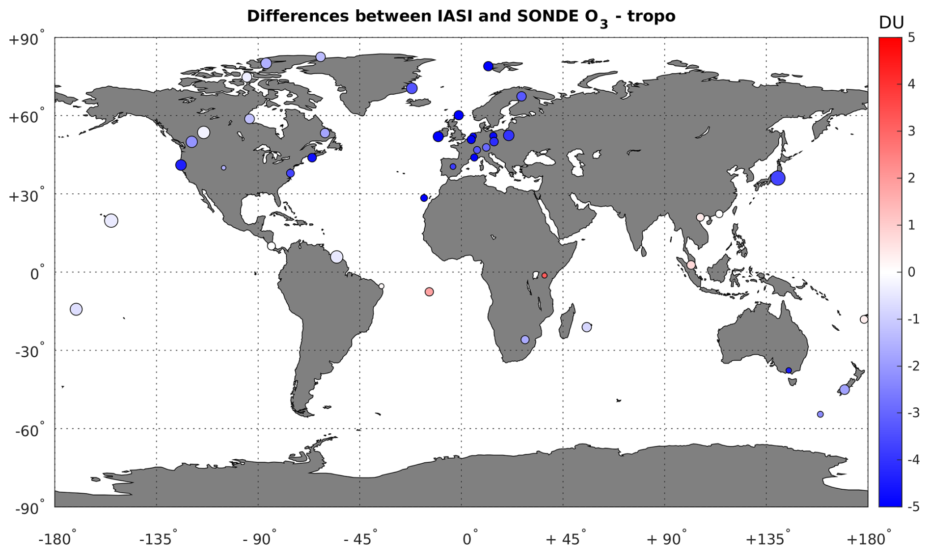
Figure 8 Location of the 43 ozonesonde stations used in this study. The colors represent the mean difference between IASI and smoothed sonde tropospheric ozone column in Dobson units (DU) over the period from January 2008 and December 2023. The standard deviation is represented by the size of the circle.

A total of 43 ozonesonde stations across midlatitudes, polar, and tropical regions, covering the period from 2008 to 2023, were considered in this study. Homogenized HEGIFTOM harmonized data were available for 37 of these sites at the time of the study, and incomplete time series were filled using WOUDC data. Only homogenized datasets were used for trend analysis, while the broader dataset was used for the IASI validation. Figure 8 shows the locations of the ozonesonde stations used in the comparison and Table 2 described the station characteristics.

2.2 Comparison methodology

Given the differences in dataset characteristics, this section outlines the comparison methodologies, collocation criteria, and statistical analysis.

2.2.1 Comparison with CrIS data

The comparison between IASI and CrIS is carried out for both total and tropospheric columns over the common time period 2016–2022. A spatial grid of 1°×1° is employed to facilitate this comparison. While this resolution might initially appear coarse, it is well suited for a global and seasonal-scale analysis. Both IASI and CrIS have native spatial resolutions of approximately 12–14 km at nadir. However, the effective resolution degrades at larger scan angles. For instance, at a 48° scan angle, the IASI footprint becomes significantly elongated due to the oblique viewing geometry, reaching up to ∼ 40 km across-track and ∼ 20 km along-track. This spatial degradation supports the use of a coarser aggregation grid. The choice of a 1°×1° grid is further justified by two main considerations. First, it ensures sufficient spatial sampling within each grid cell, which would not be guaranteed with finer resolutions, especially at global scale. Second, it enables efficient processing of large datasets while preserving the spatial representativeness needed for robust statistical analysis. Both daytime and nighttime data are included in the comparison. The differences are obtained by: [IASI − CrIS] (in DU) or [100× (IASI − CrIS)/(0.5× (IASI + CrIS))] (in percent, %), where the average of CrIS and IASI serves as a combined reference for the comparison.

2.2.2 Comparison with sonde data

Prefiltering is applied by excluding soundings that do not reach 80 hPa and those with total ozone correction factors outside the range of [0.7, 2.0]. Sonde data are aggregated into 46 pressure layers, ranging from 900 to 8 hPa, with values representing vertical averages. The averaging is performed using the midpoints between the given pressure levels.

For the comparison of IASI data with sonde measurements, profiles are paired when the sonde is launched within 1° and 6 h of the IASI measurement. The chosen thresholds ensure sufficient data for statistically meaningful comparisons and are consistent with methodologies used in previous studies (e.g., Boynard et al., 2016, 2018). These criteria can lead to multiple IASI profiles being matched to a single sonde profile.

For the validation of satellite profile products, the difference in vertical resolution has to be taken into account. In this study, for each IASI/sonde pair, the sonde profiles are interpolated onto the IASI vertical grid and degraded to the IASI vertical resolution by applying the IASI AKs and a priori O₃ profile according to Rodgers (2000):

$$\begin{array}{}\text{(1)}& x_{\mathrm{s}}=x_{\mathrm{a}}+A(x_{\mathrm{raw}}-x_{\mathrm{a}})\end{array}$$

where x_s is the smoothed ozonesonde profile, x_raw is the ozonesonde profile interpolated on the IASI vertical grid, x_a represents the IASI a priori profile and A refers to the IASI AK matrix. The sonde profiles above the burst altitude are extended using the IASI a priori profile.

For each sonde measurement, we compute the tropospheric column by using all IASI and smoothed sonde profiles that meet the coincidence criteria. Then, the IASI and smoothed sonde subcolumns are averaged, yielding one IASI-SONDE profile pair corresponding to each sonde measurement. Both IASI O₃ vertical profiles and tropospheric columns are compared against ozonesonde data. The differences are determined as: [IASI − SONDE] (in DU) or [100× (IASI − SONDE)/SONDE] (in %), where SONDE serves as a reference for the comparison. We also assess the four subcolumns defined in Boynard et al. (2018), each containing approximately one piece of information and showing maximum sensitivity around the middle of each layer. The subcolumns correspond to the following layers: surface – 300, 300–150, 150–25 and 25–3 hPa. The results are presented in Appendix A.

2.3 Trend evaluation

Trend analysis is conducted using quantile regression (QR) at the 50th percentile (median), selected for its robustness to small sample sizes, resilience to outliers, and ability to handle non-normal error distributions and autocorrelation. Following the TOAR-II statistics focus working group guidelines (Chang et al., 2023b), the monthly ozone column time series are first deseasonalized by fitting and removing a sine-cosine model with 12 and 6 month periodicities to eliminate seasonal variations. QR is then applied for trend estimation, and uncertainties and p-values are calculated using a moving block bootstrap method that accounts for autocorrelation and heteroskedasticity in the residuals. This approach is implemented using the toarstats Python package (https://gitlab.jsc.fz-juelich.de/esde/toar-public/toarstats, last access: 20 November 2024). Uncertainties in this study are reported at the 95 % confidence level (± 2σ).

Our primary trend analysis is based on the 2008–2023 period, which offers a sufficiently long time series (16 years) for robust detection of tropospheric ozone changes from both satellite and ozonesonde data. To complement this, we also compute trends over the shorter 2008–2019 window, which is used specifically as a pre-COVID reference period. This secondary time frame allows us to assess the potential influence of the COVID-19 pandemic on tropospheric ozone, but is not intended to serve as a baseline for long-term climatological trend interpretation.

Global trend calculation from IASI-CDR O₃ data is carried out on a 1° × 1° grid, considering only regions with at least 70 % of the monthly values available during the period of study. While the 1°×1° resolution is appropriate for assessing global and regional trends, it may not fully capture localized changes, particularly in urban areas where surface ozone concentrations can exhibit sharper gradients due to factors such as traffic, industrial emissions, and local meteorological conditions.

For the local trend calculation at individual sonde station, we use a different approach. We adopted selection criteria aligned with the HEGIFTOM-1 methodology (Van Malderen et al., 2025a), accounting for the limited sampling frequency at many sites (typically 2–4 profiles per week). Stations were included in the trend analysis if they recorded at least two soundings per month and had more than 50 % data coverage over the 2008–2023 period. These criteria were applied consistently to both ozonesonde measurements and satellite-sonde coincidences to ensure robust and comparable trend estimates. Based on these thresholds, 27 of the 43 available stations were retained for trend analysis. Seven of these stations are located in northern high latitudes, 11 in northern midlatitudes, eight in the tropics and one in the southern midlatitudes. Only homogenized ozonesonde time series were used to ensure consistency and reliability. Non-homogenized stations were excluded from trend estimation but remained part of the satellite validation. We also tested the sensitivity of the results to more restrictive thresholds. Increasing the requirements to at least three soundings per month and 70 % coverage did not significantly alter the derived trends for the subset of stations meeting these stricter criteria, supporting the robustness of the results under the adopted selection scheme.

In addition to this primary trend assessment over 2008–2023, we also compute trends over the shorter 2008–2019 period, used here as a pre-COVID reference window to evaluate potential pandemic-related impacts on tropospheric ozone. This secondary time frame is not intended for long-term trend assessment but serves a specific diagnostic purpose.

According to the TOAR-II statistical guidance of Chang et al. (2023b), trends have been classified by significance as follows: p-value ≤0.01 (very high certainty), $\mathrm{0.01}<p\le \mathrm{0.05}$ (high certainty), $\mathrm{0.05}<p\le \mathrm{0.10}$ (medium certainty), $\mathrm{0.10}<p\le \mathrm{0.33}$ (low certainty) and p>0.33 (very low certainty or no evidence).

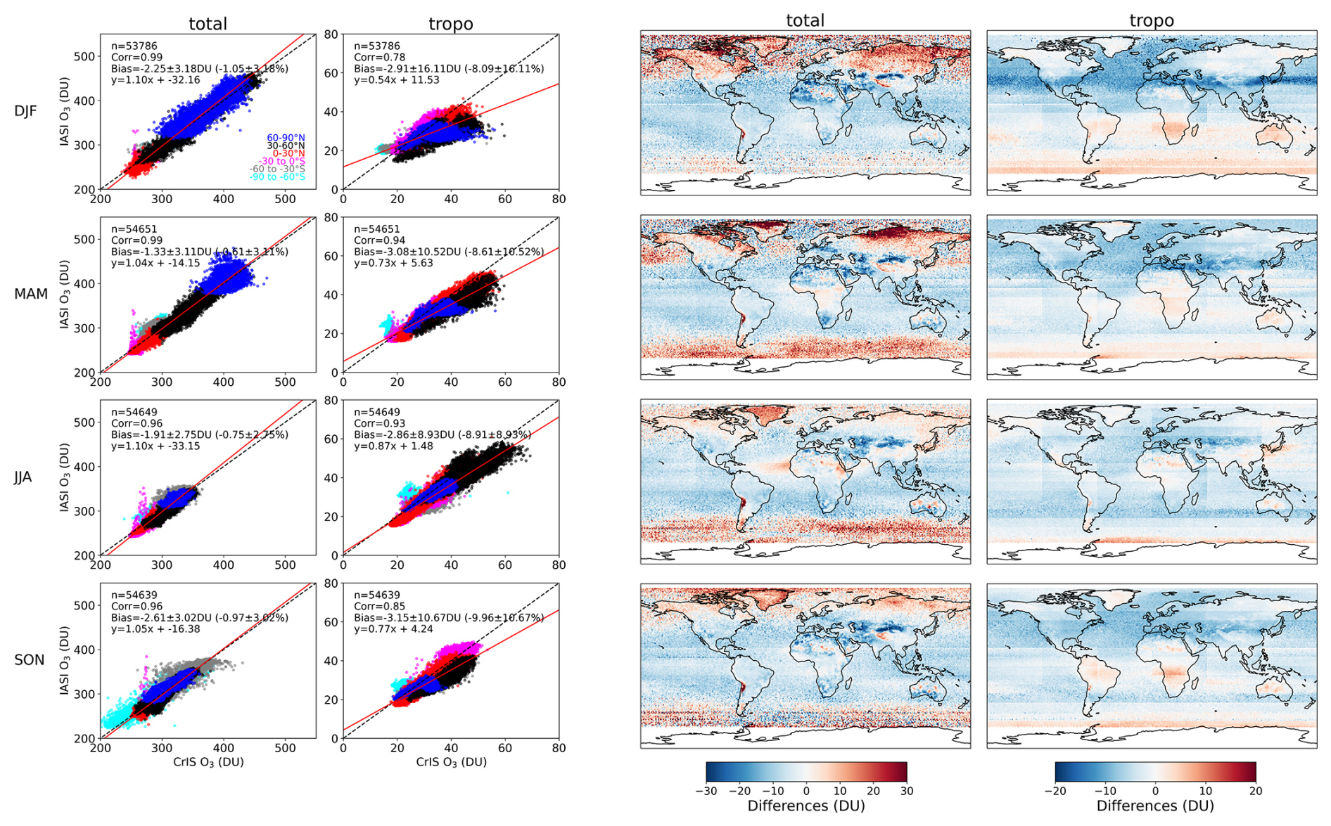
Figure 9 Left columns: Seasonal scatterplots of IASI-CDR against TROPESS-CrIS total and tropospheric ozone columns for the period 2016–2022. The color code represents different latitude bands: blue (60–90° N), black (30–60° N), red (0–30° N), magenta (0–30° S), gray (30–60° S), and cyan (60–90° S). The 1:1 line (dashed black) and the regression line (red) are shown on each scatterplot, along with statistics including the number of common grid cells, the correlation coefficient, the mean bias with standard deviation in both Dobson units (DU) and percent (%), and the linear regression. The absolute and relative biases are calculated as: IASI-CrIS and [100× (IASI-CrIS)/(0.5× (IASI+CrIS))], respectively. Right columns: Spatial distributions of the differences between CrIS and IASI total and tropospheric ozone columns (in DU). DJF, MAM, JJA and SON represent December–January–February, March–April–May, June–July–August and September–October–November, respectively. The data are averaged onto a global 1°×1° grid.

3 Validation

3.1 Comparison with CrIS data

Seasonal comparisons between IASI-CDR and CrIS-TROPESS products are conducted to evaluate their performance for two ozone columns over the period 2016–2022: total and tropospheric. The analysis includes scatterplots and spatial distribution maps, highlighting both the agreements and discrepancies between the datasets as illustrated in Fig. 9. Seasonal periods are defined as DJF (December–January–February), MAM (March–April–May), JJA (June–July–August), and SON (September–October–November).

For the total ozone column, the scatterplots show an excellent agreement between IASI-CDR and TROPESS-CrIS data, with a bias consistently below 1.2 % and correlation coefficients higher than 0.97 across all seasons. This indicates a very strong performance of both datasets in capturing total ozone variability. For the tropospheric ozone column, the differences are more pronounced, with biases ranging from 10 % to 12 % and correlation coefficients varying between 0.77 during DJF (when sensitivity is lower) and 0.91 during JJA (when sensitivity is larger), reflecting a relatively weaker, yet still reasonable, agreement.

The spatial distribution analysis provides further insights into these discrepancies. For the total ozone column, CrIS systematically underestimates ozone concentrations at northern high latitudes and in the southern midlatitudes, while overestimating ozone in the tropics across all seasons. The differences are larger in DJF and lower in JJA, when IASI and CrIS sensitivities are lower and higher, respectively. In the case of the tropospheric ozone column, CrIS tends to underestimate ozone levels across most regions, with the notable exception of a prominent red band at the southern midlatitudes, reflecting the overestimation pattern seen in the total ozone column. This specific feature may represent the impact of persistent cloud cover on the CrIS sensitivity and therefore retrieval. The differences in tropospheric ozone columns between IASI and CrIS are partly driven by the a priori information used in each retrieval, which is fixed for IASI and variable (both in latitude and season) for CrIS. This is illustrated in Fig. B1 in Appendix B, which shows similar patterns to the observed differences.

To further assess the role of a priori assumptions, we performed a sensitivity test by applying the IASI a priori fixed in latitude and not seasonally resolved, within the TROPESS retrieval framework. While the choice of a priori clearly influences the retrieved ozone columns, the resulting differences between IASI and TROPESS retrievals are smaller than the differences between their original a priori profiles. Notably, applying the IASI a priori within TROPESS produces spatial differences across the globe that do not consistently align with the spatial differences seen between the original TROPESS and IASI products. This suggests that the a priori contributes to the discrepancies but does not fully explain them. Moreover, as shown by Kulawik et al. (2008), the retrieval process is not strictly linear with respect to the a priori, implying that a full re-retrieval is needed to fully assess its impact. Additional methodological differences, such as in the treatment of prior covariance matrices and vertical profile structure, likely also play a significant role in the observed inconsistencies. Additional sensitivity studies are planned to further explore the impact of different a priori assumptions on the retrievals and gain a deeper understanding of how they influence the datasets. Overall, while the performance of both datasets is excellent for total ozone, the tropospheric ozone comparisons highlight areas requiring further investigation, particularly regarding the systematic biases observed in the southern midlatitudes.

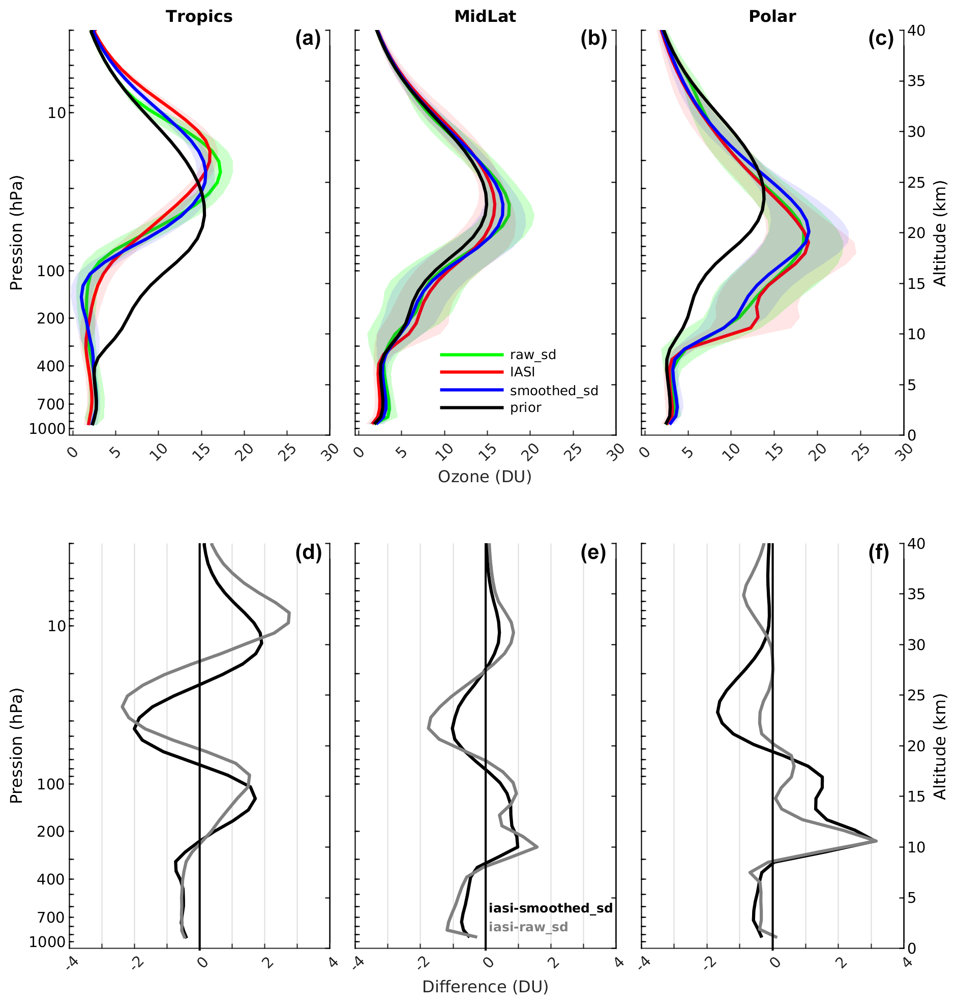
Figure 10 (a, b, c) Mean ozone vertical profiles in Dobson units (DU) retrieved by IASI (red), measured by the sondes (green), and measured by the sondes after applying the IASI averaging kernels (blue) for three latitude bands: tropics (30° S–30° N), midlatitudes (30–60° North and South) and polar regions (60–90° North and South). Shaded areas indicate the standard deviation around each mean ozone vertical profile. The black line indicates the a priori ozone profile used in the IASI retrievals; (d, e, f) vertical distribution of the differences in DU between the IASI retrieved mean profile and the smoothed sonde mean profile (black), as well as between the IASI retrieved mean profile and the raw sonde mean profile (gray).

3.2 Comparison with ozonesonde data

3.2.1 Vertical profile characterization

Figure 10 (top panels) presents a comparison of the mean retrieved IASI, smoothed, and raw sonde profiles across three latitude bands, representing the tropics, midlatitudes, and polar regions, based on all IASI-sonde coincidences from the 16-year period (2008–2023). The top panels show that IASI effectively captures the main features of the ozonesonde vertical distribution, including: (i) ozone peaks around 20–30 km, varying with latitude, (ii) a downward shift in the altitude of the ozone maximum as latitude increases, and (iii) pronounced ozone gradients at the boundary between the troposphere and the stratified lower stratosphere. Additionally, a secondary smaller peak around 200 hPa appears in IASI data over polar regions but is not consistently seen by ozonesondes. Likely linked to stratosphere-troposphere exchange, it may result from polar vortex dynamics in winter and early spring. Since IASI data are averaged over a 1° area around the sonde station, it captures greater spatial and temporal variability, possibly detecting stratosphere-troposphere exchange events that sondes, with single-time profiles, may miss. Further analysis is needed to confirm its origin.

While IASI struggles to accurately represent the gradient toward the tropopause and the ozone peak, particularly in the tropics, it successfully captures the peak amplitude and changes in vertical gradients. This issue is less pronounced in the midlatitudes and polar regions. However, the variability across different latitude bands becomes evident when analyzing the standard deviations. As noted, variability is significantly lower in the tropics compared to the mid and high latitudes. This pattern aligns with the more stable atmospheric conditions in the tropics, where ozone distribution remains relatively uniform. In contrast, the mid and high latitudes experience greater fluctuations due to more dynamic atmospheric processes, such as stronger circulation patterns and seasonal changes. These factors contribute to higher variability in ozone profiles, especially in the higher latitudes.

Figure 10 (bottom panels) illustrates the differences in ozone concentration (in Dobson units, DU) between the IASI retrieved and sonde profiles, both raw and smoothed. IASI shows lower O₃ values in the troposphere and middle stratosphere, while overestimating O₃ in the upper troposphere and lower stratosphere (UTLS) throughout all latitude regions. Potential factors contributing to the increased bias in the UTLS include the limited vertical resolution of IASI, spectroscopic uncertainties related to ozone absorption lines, or the use of inadequate a priori information (Boynard et al., 2016). Specifically, the effect of using a priori constraints that change with latitude still needs to be explored further. In the tropics, smoothing the sonde data reduces differences compared to the raw data, particularly in the stratosphere, and introduces a vertical shift of a few kilometers downward. However, in the UTLS, the differences remain unchanged. At midlatitudes, the differences between IASI and sonde profiles are generally smaller than those observed in the tropics. Additionally, the differences are less pronounced when comparing IASI data to the smoothed sonde profiles, suggesting that smoothing helps to reduce some of the variability and improve agreement with IASI data in this region. In the polar regions, differences between IASI and sonde profiles begin to diverge above 200 hPa, with larger discrepancies between IASI and the smoothed sonde than the raw sonde. This results from IASI limited vertical sensitivity, which is further reduced in cold conditions due to weaker radiance signals, increasing reliance on the a priori. Applying the averaging kernel (AK) smooths the sonde to IASI resolution but also incorporates a priori biases, especially where retrievals are poorly constrained, such as above the tropopause. In contrast, in midlatitudes and the tropics, differences between IASI and the raw sonde are generally larger. In the tropics, the IASI–raw sonde difference profile shifts upward relative to the smoothed sonde difference, likely reflecting the AK smoothing and a less representative a priori. The figure highlights regional variations in the alignment between IASI and sonde data, emphasizing the impact of smoothing on data comparison. These differences underscore the importance of a priori assumptions in the retrieval process, especially in the tropics, where low ozone variability and unique atmospheric conditions make the retrieval particularly sensitive to these assumptions. Further refinement of a priori constraints is necessary in the tropics to reduce biases, and smoothing is essential in improving agreement between IASI and sonde data, particularly in regions with more variable ozone profiles, such as the midlatitudes.

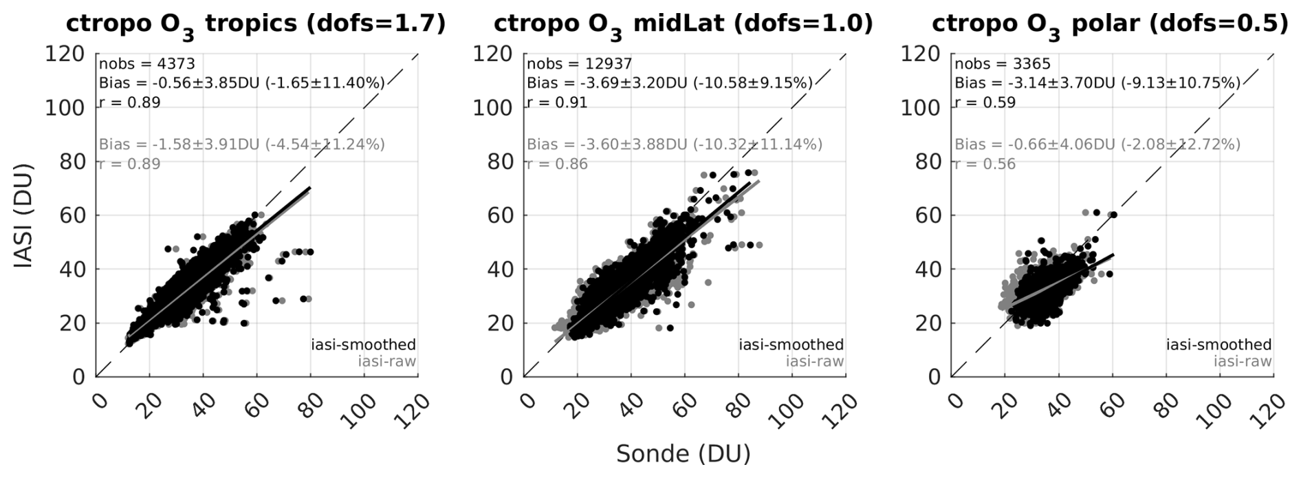
Figure 11 Comparison of IASI with raw (gray) and smoothed (black) sonde tropospheric ozone subcolumns for the period 2008–2023, shown across three latitude bands: tropics (30° S–30° N), midlatitudes (30–60° North and South) and polar regions (60–90° North and South). The 1:1 line (dashed) and the regression lines (black for smoothed, gray for raw) are shown on each scatterplot, along with statistics including the number of collocations, mean bias with standard deviation in both Dobson units (DU) and percent (%), correlation coefficient (r), and the associated mean Degrees of Freedom for Signal (DOFS).

3.2.2 Tropospheric ozone statistical analysis

Figure 11, illustrating the scatterplots between IASI and smoothed sonde data, shows that IASI underestimates the tropospheric ozone column, with biases ranging from −2 % in the tropics to −10 % in the midlatitudes and polar regions (see Fig. 8 for the spatial distribution of the bias). The standard deviation is about 11 % across all latitude bands, indicating a consistent level of variability in the measurements. The correlation coefficient is high (0.9) in both the tropics and the midlatitudes, suggesting strong agreement between IASI and sonde concentrations, but drops to 0.6 in the high latitudes, indicating weaker performance in the polar regions, which is due to limited signal in those regions (DOFS =0.5). The DOFS are 1.7 in the tropics and 1 in the midlatitudes, reflecting better retrieval of information in those regions. The number of observations is 2–3 times higher in the midlatitudes compared to the tropics and the high latitudes, which could contribute to the more robust results in those regions. The comparison between IASI and raw sonde data also included in Fig. 11 shows similar results to the comparison with smoothed sonde data, although it exhibits a larger bias in the tropics and a lower bias in the polar regions. The higher bias observed with smoothing in the polar regions may be due to the loss of important temperature and humidity variability, while the lower bias in the tropics could result from the more stable atmospheric conditions, which are better captured by smoothing.

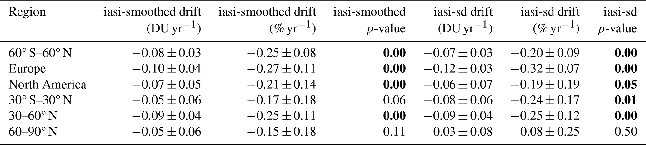
Table 3 Tropospheric ozone drifts derived from IASI and ozonesonde data (smoothed and raw) over 2008–2023 on both global and regional scales. The thermal tropopause is estimated using the World Meteorological Organization thermal definition (WMO, 1957). Uncertainties are reported at the 2σ level. P-values ≤0.05 are shown in bold.

3.2.3 Tropospheric ozone temporal stability assessment

The temporal stability of the IASI tropospheric ozone product is assessed by analyzing drift, defined as the difference between IASI tropospheric ozone retrievals and both smoothed and raw ozonesonde measurements over the 2008–2023 period. Drift analysis uses the same median quantile regression methodology, significance classification, and selection criteria as trend estimation (see Sect. 2.3), ensuring consistency in both approaches. Except in the tropics (30° S–30° N) and northern high latitudes (60–90° N), drift derived from comparisons with smoothed ozonesonde data is estimated with high certainty (p-value ≤0.01) both globally and regionally, but remains below 3 % per decade (see Table 3), meeting the stability criterion recently cited for tropospheric ozone observations (Weber, 2024). These results indicate that the IASI product is generally stable and suitable for long-term trend assessment. However, although the drift values remain below 3 % per decade, the high certainty of the estimates underscores the need for continuous monitoring to ensure their long-term stability.

In the tropics and northern high latitudes, where p-values indicate medium to low statistical significance (p>0.05), drifts based on smoothed sonde comparisons are not statistically significant, further supporting the IASI temporal stability. Comparisons with raw ozonesonde data show drift magnitudes comparable to those from smoothed data, generally below the 3 % per decade threshold but often with higher statistical significance. This pattern likely reflects the influence of short-term atmospheric variability and measurement noise in the raw profiles, rather than a systematic bias in the satellite record.

An analysis at individual stations over the 2008–2023 period reveals several sites with significant IASI–ozonesonde drifts exceeding the 3 % per decade stability threshold (Table S1). Stations such as Payerne, OHP, Lauder, and Reunion exhibit statistically significant negative drifts despite having continuous, well-sampled records, supporting the robustness of these results. The drift observed between IASI and ozonesonde data at Payerne and OHP likely reflects ozonesonde-specific issues rather than satellite bias or altitude effects. Despite homogenization, residual uncertainties remain, particularly at those stations, where sonde trends show inconsistencies with other techniques during certain periods (Van Malderen et al., 2025a). These differences may be explained by local data processing and regional variability, which can impact trend agreement across datasets. At Lauder, where no known instrumental changes occurred and coverage exceeds 90 %, the drift may reflect regional representativeness issues or limitations in satellite sampling over the Southern Hemisphere. In contrast, stations like Churchill and Kelowna also show relatively large drifts but suffer from limited temporal coverage due to data gaps or truncated time series, which may reduce the reliability of the estimates. These cases underscore the importance of data continuity when interpreting station-level drifts and their contribution for regional trend assessments.

We also tested the sensitivity of the results to more restrictive thresholds. Increasing the requirements to at least three soundings per month and 70 % coverage resulted in a smaller drift for the subset of stations meeting these stricter criteria, with the drift decreasing from −2.5 % to −1 % per decade. This supports the robustness of the results while showing that stricter criteria lead to a lower drift estimate. Additionally, incomplete time series, with gaps or early terminations, impact the drift, potentially introducing more variability in the results. Therefore, caution is needed when interpreting the drift derived from the less restrictive criteria.

Overall, the drift analysis indicates that the IASI tropospheric ozone product is temporally stable over the 2008–2023 period, with most stations showing drifts within the 3 % per decade threshold. To ensure consistency, we tested the impact of including stations with significant drift in the regional trend analysis. Results showed that, whether or not these stations were included, the overall global and regional trend estimates remained unchanged. Therefore, all stations were considered in the global and regional trend analysis.

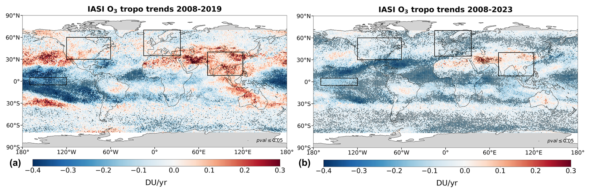
Figure 12 Spatial distribution of tropospheric ozone trends (in DU yr⁻¹) derived from IASI-CDR before the COVID-19 pandemic (2008–2019; a) and including the pandemic (2008–2023; b). The tropospheric column is integrated from the surface to the thermal tropopause, as defined by the World Meteorological Organization (WMO, 1957). Dots indicate trends with high to very high certainty (p-value ≦0.05). The black rectangles indicate the boundaries of the regions analyzed in Fig. 13.

4 Trends analysis

4.1 Tropospheric O₃ trends

4.1.1 Global and regional patterns

Figure 12 shows the spatial distribution of tropospheric ozone trends from IASI data for two periods: 2008–2019 (before the COVID-19 pandemic) and 2008–2023 (including the pandemic). The results show distinct patterns across the two periods analyzed. From 2008 to 2019, ozone concentrations decrease primarily in the tropics, with increases in certain regions, such as over parts of the Pacific around 30° N and 30° S, in the Arabian Peninsula and in Asia. Extending the analysis to 2008–2023 reveals that the negative trends observed in the tropics and Europe persist or become more pronounced, while the previously positive trends over the Arabian Peninsula and parts of Asia weaken but remain slightly positive. The impact of the 2020 lockdowns, which led to a reduction in ozone precursors (NO_x and VOCs), likely contributed to a decrease in ozone production. However, regional emissions and other factors may help explain the continued positive ozone trends in the Arabian Peninsula and North China Plain (NCP). This finding in Asia agrees with Dunn et al. (2024) who found the strongest positive trends above South and East Asia over 2004–2023, based on OMI-MLS observations.

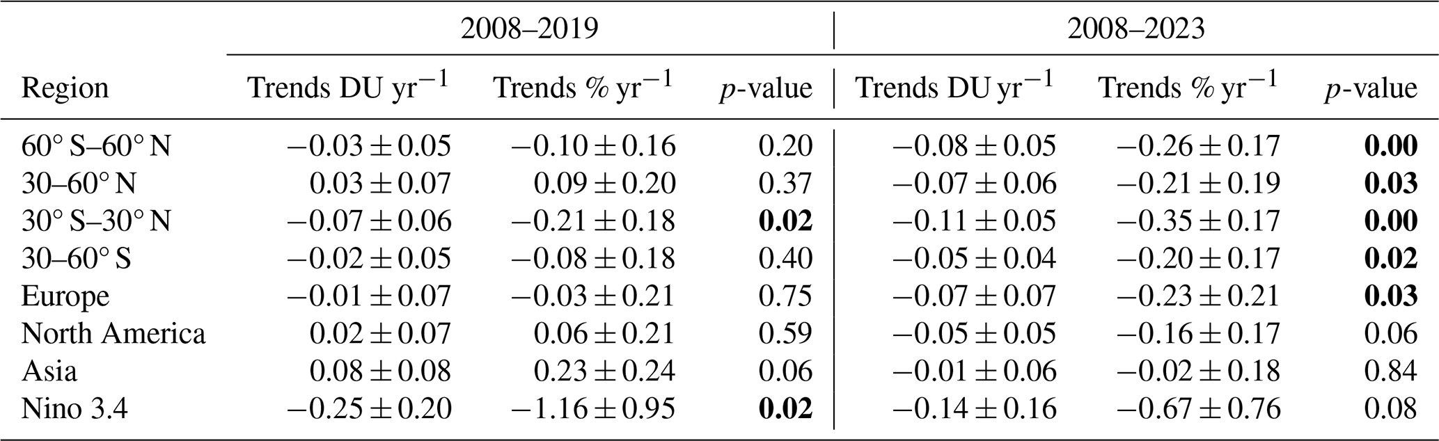
Table 4 Tropospheric ozone trends derived from IASI-CDR before the COVID-19 pandemic (2008–2019) and including the pandemic (2008–2023), on both global and regional scales. The thermal tropopause is estimated using the World Meteorological Organization thermal definition (WMO, 1957). Uncertainties are reported at the 2σ level. P-values ≤0.05 are shown in bold.

Extending the trend analysis using quantile regression at the 90th and 95th percentiles over 2008–2023 offers further insight into ozone behavior, especially regarding extreme ozone episodes. As shown in Figure C1 (Appendix C), biomass burning regions such as South America, South Asia, Indonesia, and Australia show near-zero or slightly negative median (50th percentile) ozone trends, but positive trends at higher percentiles, indicating an increased frequency or intensity of extreme events linked to episodic biomass burning. In contrast, other regions generally display consistent negative trends across all quantiles. These results highlight the complexity of regional ozone dynamics: while average ozone concentrations may decline due to structural changes in emissions and climate variability, extreme ozone events can persist or even intensify in some regions. This underscores the importance of considering both mean and extreme values when assessing tropospheric ozone trends.

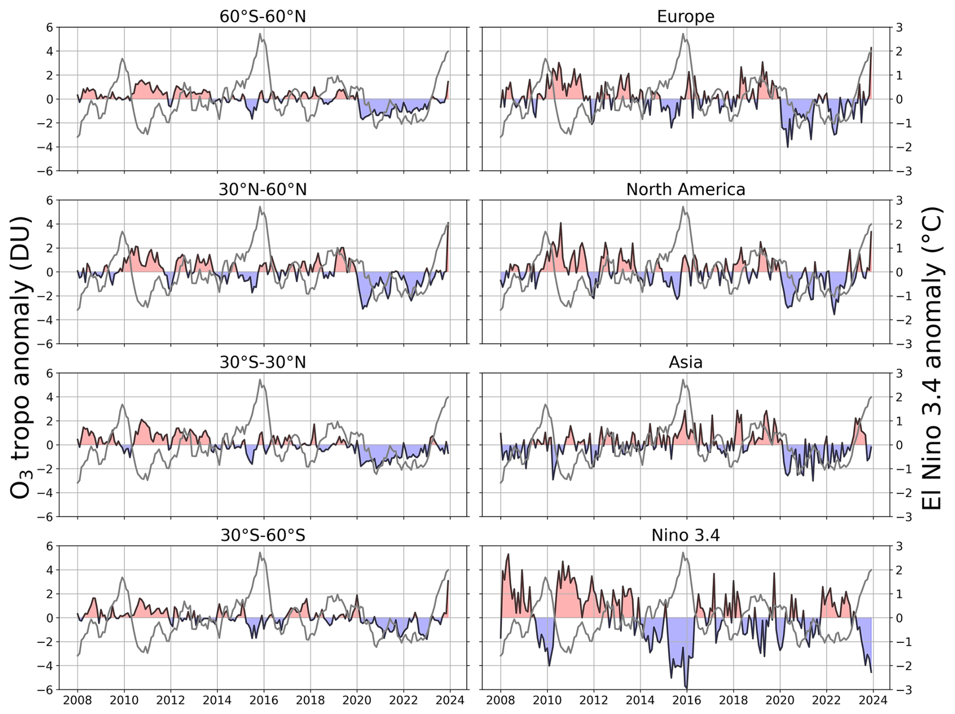
Figure 13 Monthly time series of tropospheric ozone anomalies (in DU) derived from IASI-CDR for different regions. The monthly El Niño 3.4 index is overlaid in gray for comparison. The tropospheric column is integrated from the surface to the thermal tropopause, as defined by the World Meteorological Organization (WMO, 1957).

4.1.2 Temporal patterns and statistical analysis

To better characterize the spatial distribution of tropospheric ozone trends, Fig. 13 shows the monthly anomalies derived from the IASI-CDR product across different latitude bands and regions (see Fig. 12 for region definitions). A notable feature is the widespread negative ozone anomalies starting in 2020, persisting through 2023 in most regions except the Niño 3.4 region. This decrease coincides with reduced emissions of ozone precursors in the Northern Hemisphere resulting from COVID-19 lockdown restrictions (Ziemke et al., 2022). These negative anomalies partially explain the observed negative trends over the 2008–2023 period, with varying levels of statistical certainty reported in Table 4: high in the northern and southern midlatitudes (p≤0.05) and very high in the tropics (p≤0.01). Another factor contributing to the persistence of the negative anomaly is the occurrence of three consecutive years of La Niña conditions in the tropical Pacific Ocean from mid-2020 to early 2023, followed by a rapid transition to ENSO-neutral and El Niño conditions by May 2023 (Dunn et al., 2024). The El Niño 3.4 index for 2008–2023 is also shown in Fig. 13 (gray line). An anti-correlation between La Niña events and ozone anomalies is evident in the Niño 3.4 region, indicating a strong climatic influence on ozone variability, a pattern not observed in other regions. As shown in Table 4, for the earlier period 2008–2019, trends show low to very low certainty overall, except in Asia, where a positive trend of +0.23 ± 0.24 % yr⁻¹ with medium certainty (p=0.06) was found, and in the tropics, where a negative trend of −0.21 ± 0.18 % yr⁻¹ was detected (p=0.02; high certainty).

The negative ozone anomalies observed since 2020 coincide with substantial reductions in precursor emissions due to COVID-19 lockdowns. Several studies report significant decreases in NO_x and VOC emissions during this period. For example, in Indian cities, NO₂ levels dropped by over 70 % and VOC concentrations by more than 80 % during the initial lockdowns (Pakkattil et al., 2021). These changes impacted ozone production differently depending on local chemical regimes: in VOC-limited areas, reduced NO_x emissions decreased ozone titration by NO, potentially increasing ozone concentrations, whereas in NO_x-limited regions, simultaneous decreases in NO_x and VOCs led to lower ozone formation (Miyazaki et al., 2021; Nussbaumer et al., 2022). As economic activity resumed, precursor emissions, especially NO_x, rebounded in many regions, resulting in a partial recovery of surface ozone concentrations, particularly over North America (U.S. EPA, 2024). However, IASI data indicate that free tropospheric ozone anomalies remained negative through 2023 across most regions, suggesting a decoupling between surface and free tropospheric ozone behavior, likely influenced by vertical transport and regional dynamics.

Recent studies corroborate these observations, reporting short-term ozone reductions linked to COVID-19 restrictions. Pimlott et al. (2024) report an 11 %–15 % decrease in European lower tropospheric ozone from 2020 to 2022, with the largest declines occurring in 2022, suggesting additional influencing factors beyond the pandemic. Nelson and Drysdale (2025) observed a marked drop in NO₂ concentrations across Europe around 2020, with some rebound following easing of restrictions. In tropical regions, Thompson et al. (2025) note that COVID-19 slightly moderated recent ozone trends, reflecting broader atmospheric responses to emission changes.

Beyond the pandemic, the overall ozone decline from 2008 to 2023 likely results from multiple factors, including stricter environmental regulations, improved land and fire management, particularly in Indonesia, India, and China (Kashyap et al., 2024), and persistent La Niña conditions (2020–2023), which suppressed fire activity and reduced emissions of ozone precursors such as carbon monoxide and VOCs in affected regions (Zhu et al., 2021; Zheng et al., 2021; Xie et al., 2025).

A comparison with Dufour et al. (2025), who analyzed IASI-O3 KOPRA data from 2008 to 2022 using similar regional definitions, shows general consistency in key areas. Both studies identify a high-certainty negative trend over Europe (−0.07 ± 0.07 DU yr⁻¹, p=0.03 in this study; −0.05 ± 0.02 DU yr⁻¹ with 1σ uncertainty, p=0.03 in Dufour et al., 2025). Over North America, both studies detect a negative trend, though with medium to low certainty (−0.05 ± 0.05 DU yr⁻¹, p= 0.06 in our study; −0.03 ± 0.03 DU yr⁻¹ with 1σ uncertainty, p= 0.34 in Dufour et al., 2025). In Asia, neither study finds a significant trend (−0.01 ± 0.06 DU yr⁻¹, p=0.84 in our study; −0.05 ± 0.03 DU yr⁻¹ with 1σ uncertainty, p=0.16 in Dufour et al., 2025).

4.2 Lower versus upper tropospheric O₃ trends

When examining trends in the upper (450 hPa–tropopause) and lower (surface–450 hPa) troposphere for the periods 2008–2019 and 2008–2023 (see Figs. D1 and D2 in Appendix D), negative trends with high certainty (p≤0.05) are consistently observed in the lower troposphere for both periods. Over arid and desert regions, such as parts of Africa and Australia, retrievals may be affected by surface emissivity issues (Boynard et al., 2018), potentially introducing biases in the trend estimates. Therefore, the positive trends observed in these regions should be interpreted with caution.

The upper troposphere presents a more complex picture: from 2008 to 2019, positive trends with high certainty are evident in several midlatitude regions, including the North Pacific Ocean, North Atlantic Ocean, Asia, and the Mediterranean, while negative trends with high certainty are observed in the tropical Pacific Ocean. From 2008 to 2023, most regions exhibit weaker ozone trends, except for the North Pacific Ocean, the Arabian Peninsula, and the NCP, where positive trends with high certainty are observed. These upper-tropospheric increases are consistent with OMI-MLS trends reported by Dunn et al. (2024) and Pope et al. (2024), who highlight ozone increases over South and East Asia since the early 2000s. These findings also align with Dufour et al. (2025), who reported negative trends with high certainty in the lower troposphere and trends with low to medium certainty in the upper troposphere, except over China, using on IASI-O3 KOPRA data from 2008 to 2022.

In the upper troposphere, the tropics generally exhibit persistent negative trends in ozone, except in areas affected by recurrent fires which show a different behavior. In these regions, ozone levels can increase due to the release of large amounts of CO and VOCs during fires, which trigger photochemical reactions that produce ozone, particularly in the presence of sunlight. This phenomenon is especially pronounced in the upper troposphere, where ozone formation is more sensitive to photochemical processes. Moreover, the upward transport of pollutants from fires can lead to an accumulation of ozone in the upper troposphere, contributing to the observed trends in these regions. In addition, the long-range transport of ozone precursors, particularly within the free troposphere, further amplifies these trends, as highlighted by Glotfelty et al. (2014) and Itahashi et al. (2020). At mid and high latitudes, the observed positive trends in the upper troposphere may reflect stratospheric influences possibly due to transport processes, such as stratosphere-troposphere exchanges (Luo et al., 2024b), but biomass burning and long-range transport can also contribute.

Separating the surface–450 hPa and 450 hPa–tropopause columns provides valuable insights, as it reveals decreasing ozone trends in the lower troposphere, while trends in the upper troposphere are more mixed, influenced by factors such as the transport of ozone precursors.

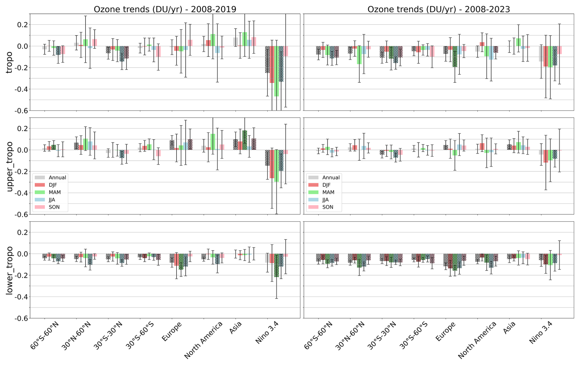
Figure 14 Tropospheric ozone annual and seasonal trends (in DU yr⁻¹) derived from IASI-CDR for different subcolumns (full, lower and upper tropospheric column) before the COVID-19 pandemic (2008–2019, left) and including the pandemic (2008–2023, right). The full, lower and upper tropospheric columns are defined as follows: surface to thermal tropopause, surface to 450, and 450 hPa to thermal tropopause, respectively. The thermal tropopause is estimated using the World Meteorological Organization thermal definition (WMO, 1957). Uncertainties are reported at the 2σ level. Hatchings indicate trends with high to very high certainty (p-value ≤0.05).

4.3 Seasonal and annual trends: full, upper, and lower tropospheric O₃

Figure 14 shows the annual and seasonal trends in tropospheric ozone over the two periods of study (2008–2019 and 2008–2023) for different regions and three tropospheric columns: full (following the WMO thermal definition), lower (surface to 450 hPa) and upper (450 hPa to thermal tropopause) troposphere.

Over the period 2008–2019, no seasonal trend in tropospheric ozone is found for all regions, except in the tropics and the Niño 3.4 region, where negative trends with high certainty are found in JJA and SON (tropics) and in JJA (Niño 3.4), respectively. In the tropics, the annual trend in tropospheric ozone is driven by contributions from both the lower and upper troposphere in JJA, and solely by the lower troposphere in SON. In the Nino 3.4 region, the annual trend is primarily influenced by the upper troposphere in JJA. Interestingly, in the Niño 3.4 region during MAM, the tropospheric column does not exhibit a significant trend, yet the lower troposphere shows a statistically significant negative trend, while the upper troposphere remains non-significant. In contrast, in the tropics during SON, the tropospheric column shows a significant negative trend, which is entirely driven by the lower troposphere, with no contribution from the upper layer. These examples highlight the value of separating vertical layers when assessing seasonal ozone trends, as trends in the full column may not accurately reflect the distinct behaviors occurring within individual layers.

Over the period 2008–2023, trends in the upper troposphere are less positive, while those in the lower troposphere are more negative across all regions. This results in more negative trends in the full tropospheric ozone column compared to 2008–2019. A negative trend with high certainty in the full tropospheric ozone column is found in MAM and SON in Europe and North America, respectively. Asia shows no annual and seasonal trend for the full tropospheric column over 2008–2023. During 2008–2019, positive annual trends are observed with low to very low certainty, primarily driven by high-certainty positive trends in the upper troposphere during MAM and SON. For both periods, trends with low to very low certainty in the full tropospheric column are generally due to compensating positive and negative trends in the upper and lower troposphere, respectively.

Table 5 Tropospheric ozone trends derived from IASI and ozonesonde data (smoothed and raw) over 2008–2023 on both global and regional scales. The thermal tropopause is estimated using the World Meteorological Organization thermal definition (WMO, 1957). Uncertainties are reported at the 2σ level. Uncertainties are reported at the 2σ level. P-values ≤0.05 are shown in bold.

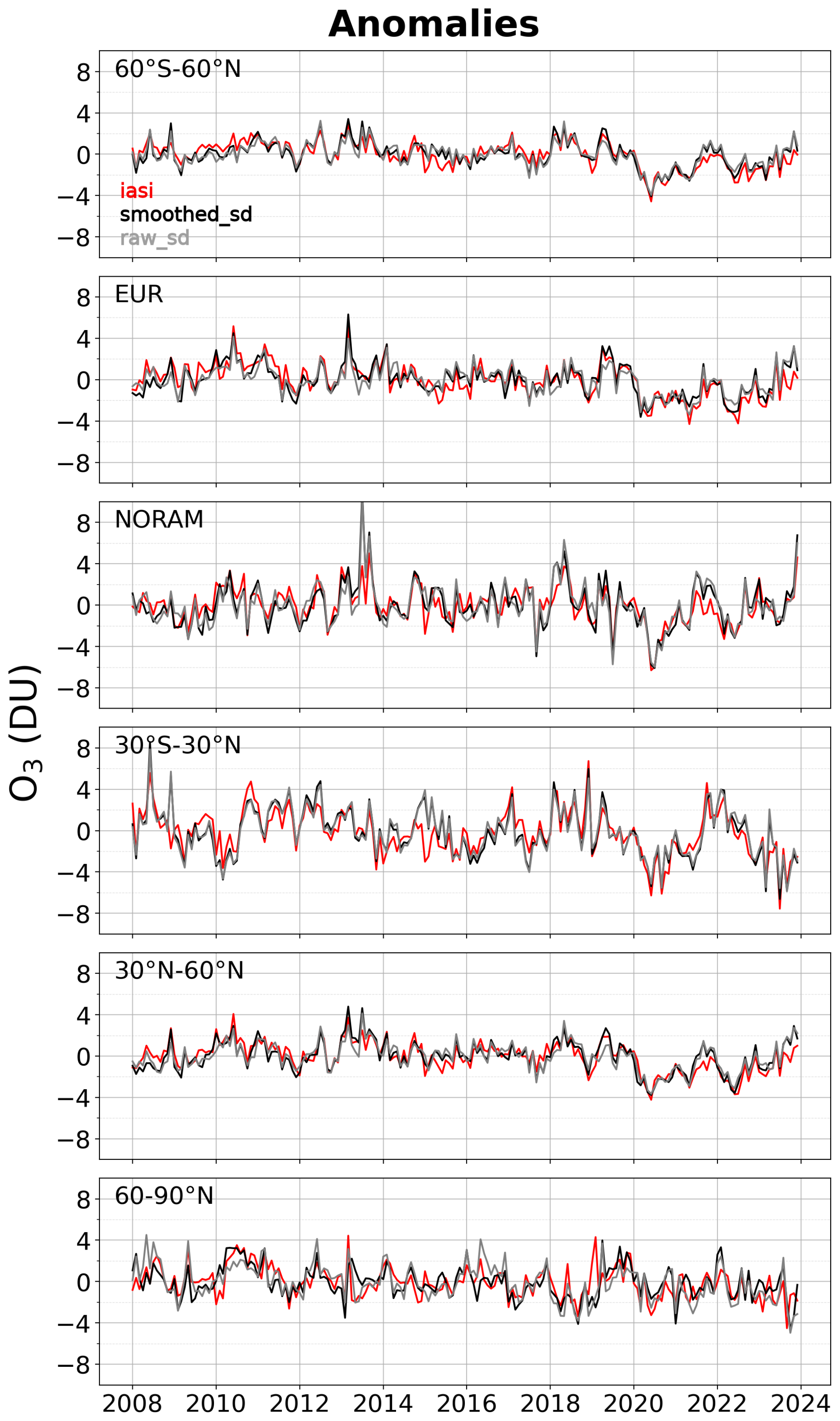
Figure 15 Monthly time series of tropospheric ozone anomalies in Dobson units (DU) derived from IASI CDR (red), smoothed (black) and raw (gray) sonde data on the global and regional scales. The tropospheric column is integrated from the surface to the thermal tropopause, as defined by the World Meteorological Organization (WMO, 1957).

4.4 Comparison with ozonsonde data

4.4.1 Regional trends

To assess the tropospheric ozone trends derived from IASI data, we compare them with trends calculated from sonde data. As described in Sect. 2.3, only ozonesonde stations with at least two observations per month (enabling reliable monthly mean calculations) and a minimum of 50 % data coverage over the period of study are included in the trend analysis which results in a total of 27 stations. Furthermore, since the exclusion of stations exhibiting drift does not significantly affect the estimated trends, all stations, regardless of drift, were included in the global and regional trend calculations to maximize spatial coverage.

Figure 15 illustrates the monthly time series of tropospheric ozone anomalies derived from IASI observations, along with both raw and smoothed sonde data, for the global and regional scales during the 2008–2023 period. It shows a strong agreement in the temporal variability of tropospheric ozone anomalies between IASI and smoothed sonde data on both scales. A pronounced drop in tropospheric ozone is observed in 2020, coinciding with the COVID-19 pandemic. As shown in Table 5, negative trends in tropospheric ozone are observed at the global scale, with IASI showing a stronger decline (−0.16 ± 0.08 DU yr⁻¹; p=0.00) and higher certainty compared to smoothed ozonesonde data (−0.05 ± 0.09 DU yr⁻¹; p=0.25). At the regional scale, both IASI, smoothed, and raw ozonesonde data show consistent negative trends with very high certainty in the tropics (30° S–30° N), with IASI showing a trend of −0.20 ± 0.15 DU yr⁻¹ and smoothed ozonesondes showing a trend of −0.20 ± 0.16 DU yr⁻¹. This strong agreement across datasets indicates a robust trend in this region. However, in the high northern latitudes (60–90° N), while IASI and raw ozonesonde data show negative trends with high certainty (−0.11 ± 0.08 DU yr⁻¹ for IASI and −0.13 ± 0.11 DU yr⁻¹ for raw ozonesondes), smoothed ozonesonde data shows a weaker and less significant trend (−0.07 ± 0.08 DU yr⁻¹; p=0.09). This difference is likely due to the IASI reduced vertical resolution and the smoothing process applied to the ozonesonde data, which diminishes its sensitivity to ozone variations, particularly in regions with more dynamic and complex ozone profiles, such as the high latitudes.

4.4.2 Local trends

2008–2023

An analysis of tropospheric ozone trends from 2008 to 2023 at the individual stations using IASI and ozonesonde data (both smoothed and raw; see Table S2) reveals predominantly negative trends, especially across northern midlatitudes and tropical regions. Several stations show strong agreement between IASI and sonde datasets, both in trend direction and statistical significance.

For example, at Scoresbysund, both IASI (−0.15 ± 0.07 DU yr⁻¹) and smoothed ozonesondes (−0.24 ± 0.07 DU yr⁻¹) exhibit consistent negative trends with high to very high certainty. Similar agreement is seen at Uccle, Costa Rica, and Paramaribo, where trends are coherent in magnitude and direction across datasets and meet at least medium significance levels. These sites provide robust evidence of tropospheric ozone decline.

In the tropics, trends are more heterogeneous. While stations like Costa Rica and Paramaribo show statistically significant declines, others, such as Samoa, Nairobi, and Hilo, exhibit negative trends with large uncertainties, limiting interpretability. This variability likely reflects regional atmospheric dynamics, local emissions, and seasonal influences. Differences in vertical sensitivity and spatial representativity between IASI and ozonesondes also contribute to the observed discrepancies.

At some high-latitude stations, differences between smoothed and raw sonde data are notable. For instance, at Ny-Ålesund, IASI shows a strong decrease (−0.21 ± 0.06 DU yr⁻¹; very high certainty), while smoothed ozonesondes show no significant trend. However, the raw sonde record reveals a significant decline (−0.16 ± 0.07 DU yr⁻¹), closely matching IASI. This highlights the potential impact of smoothing on trend magnitude and significance, especially in regions with strong seasonal variability such as the Arctic.

In contrast, at Sodankylä, IASI indicates a significant negative trend (−0.24 ± 0.08 DU yr⁻¹; very high certainty), while both smoothed and raw ozonesonde records show weak or negligible trends with low confidence. These differences may be attributed to vertical sensitivity, representativity, and trend dilution in in situ records.

Overall, the consistent trend directions and significant changes observed at multiple stations support the presence of regionally coherent declines in tropospheric ozone. However, differences in data characteristics, trend magnitudes, and significance levels across sites emphasize the importance of using multiple datasets and methods to accurately interpret local changes.

2008–2019

To complement the full-period analysis, trends were also calculated for the shorter, pre-COVID period 2008–2019 (see Table S2). As expected, these shorter-term trends show increased uncertainty and variability. However, the overall direction of trends remains consistent with the 2008–2023 results, supporting the robustness of observed ozone changes.

For 15 common stations, IASI and ozonesonde trends estimated in our study were compared with those from the HEGIFTOM dataset (see Supplement Table S3 compiles both our results and those from HEGIFTOM). Although IASI trends for this shorter period often have large uncertainties, agreement in trend direction with HEGIFTOM is seen at most locations, for example, at Boulder, Madrid, and Nairobi, where trends are broadly positive across all datasets, although statistical significance is limited. At some tropical stations (Wallops, Hilo, Paramaribo), differences in trend direction emerge but generally fall within uncertainty ranges, particularly for IASI. At Samoa, both IASI and sonde data suggest a decrease, consistent with the negative trend reported in HEGIFTOM with high certainty

Although this comparison uses the same 2008–2019 period, the differences and larger uncertainties show that trends from shorter records are less reliable. A longer period like 2008–2023 (16 years) provides more confidence, but caution is needed when interpreting trends from shorter periods, as seen with the 12-year 2008–2019 data from our study and HEGIFTOM.

5 Conclusions

This study, conducted within the framework of the TOAR-II project, aims to deepen our knowledge of the spatiotemporal patterns and trends in global tropospheric ozone, using the O₃ Climate Data Record (CDR) from the IASI/Metop (IASI-CDR). This dataset, recently reprocessed by EUMETSAT AC SAF, provides a consistent 16-year record (2008–2023) for the first time, enabling robust ozone trend analysis and contributing to our understanding of tropospheric ozone variability. The research focused on two main objectives: evaluating the quality and consistency of the IASI-CDR O₃ products and investigating the spatiotemporal variability and long-term trends in tropospheric ozone.

Key findings are summarized as follows:

Assessment of IASI-CDR ozone data:

• A comparison with CrIS-TROPESS data shows excellent agreement for total ozone (biases <1.2 %, correlations >0.97) and good agreement for tropospheric ozone (biases 10 %–12 %, correlations 0.77–0.91). However, the systematic overestimations in CrIS tropospheric ozone, particularly at high northern and southern midlatitudes, indicate the need for further investigation.

• When compared with ozonesonde data, IASI-CDR profiles generally capture the main features of vertical ozone distribution, but tend to underestimate tropospheric and stratospheric ozone, and overestimate UTLS ozone. The IASI-CDR product underestimates the tropospheric ozone column, with biases ranging from −2 % in the tropics to −10 % at mid and high latitudes.

• Drift analysis confirms the long-term temporal stability of the IASI tropospheric ozone product relative to ozonesondes, with values consistently below 3 % per decade globally and regionally, meeting the required stability criteria for trend assessment. Despite local drifts at stations like Payerne, OHP, and Lauder, caused by local data processing issues, regional variability or limited data coverage, their impact on overall trends is minimal, confirming the robustness and reliability of the IASI dataset for tropospheric ozone analysis. Continuous monitoring remains important to maintain long-term stability.

Spatiotemporal ozone variability and trends:

• Tropospheric ozone trends derived from IASI data reveal regional variability. From 2008 to 2019, ozone decreased in the tropics (−0.20 % yr⁻¹), but increased in localized regions like North Pacific Ocean, Asia and the Arabian Peninsula. Over the extended period (2008–2023), negative trends became more pronounced, particularly in the tropics and in Europe, while positive trends weakened, persisting only in areas like the Arabian Peninsula and North China Plain.

• Vertical and seasonal analyses indicate that ozone reductions are strongest in the lower troposphere. Positive trends in the upper troposphere are largely confined to regions affected by biomass burning and pollutant transport, such as South and East Asia. These upper-level positive trends are reported with medium certainty. The tropical upper troposphere, in contrast, shows persistent ozone declines, reinforced by La Niña events during 2020–2023, reduced fires and COVID-related emission cuts (Ziemke et al., 2022; Miyazaki et al., 2021).

• Quantile regression analyses reveal that while median tropospheric ozone levels decreased, the frequency of extreme ozone events (90th and 95th percentiles) increased in biomass burning regions, notably in South Asia. This suggests that despite an overall decline in average ozone, episodes of elevated ozone concentration persist or even intensify in these areas.

• Globally, IASI-CDR indicate a significant decline in tropospheric ozone with very high certainty (−0.08 ± 0.05 DU yr⁻¹; p=0.00). At the regional level, the strongest and most robust declines are found over the tropics, Europe, and the high northern latitudes. Trends over North America and Asia are also negative but with lower certainty. These findings are broadly supported by comparisons with co-located ozonesonde data. While statistical significance in sonde-based trends is generally lower, particularly at midlatitudes, high-certainty decreases are consistently found in the tropics across all datasets (IASI, smoothed sonde, and raw sonde profiles).

Comparison with other observational records:

• A comparison of 2008–2019 trends at 15 common ozonesonde stations with the HEGIFTOM dataset (see Table S3 in the Supplement) shows general agreement in trend direction across IASI, ozonesonde, and HEGIFTOM data, particularly at sites like Boulder, Madrid, and Nairobi. However, discrepancies at some tropical stations (e.g., Wallops, Hilo) and the larger uncertainties associated with the shorter time series highlight the limitations of decadal-scale trend estimates. These findings underscore the value of the 16-year record (2008–2023) for more robust and consistent assessments.

• Comparison with Dufour et al. (2025) shows overall agreement on negative tropospheric ozone trends in northern midlatitudes, particularly over Europe (high certainty) and weaker or uncertain trends over North America and Asia.

• Over the period 2008–2023, our analysis shows that negative trends in the tropospheric ozone column derived from IASI mainly result from decreases in the lower troposphere, while regionally positive trends are observed in the upper troposphere. This finding contrasts with the generally positive or stable trends reported by UV instruments (e.g., OMI, GOME-2) and long-term in situ records covering longer timeframes (e.g., 1990–2019; 1998–2023) (Gaudel et al., 2024; Elshorbany et al., 2024; Thompson et al., 2025). A factor contributing to these discrepancies is the differing temporal coverage of the datasets. IASI captures trends starting in 2008, a period marked by stricter emission controls in industrialized regions, likely reducing ozone precursors such as NO_x and VOCs. In contrast, OMI and in situ data span earlier periods when emissions in emerging economies were rising, potentially masking recent declines. This discrepancy highlights the importance of aligning the analysis period across observational datasets to ensure a meaningful comparison of trends.

• When trends are analyzed by vertical layer, two clear patterns emerge. In the lower troposphere (surface–450 hPa), negative trends with high certainty dominate across the tropics and northern midlatitudes, for both 2008–2019 and 2008–2023 periods, consistent with the findings of Pimlott et al. (2024) based on vertically resolved UV data. Conversely, the upper troposphere (450 hPa–tropopause) shows positive trends over Asia, aligning with recent UV-based studies (e.g., Dunn et al., 2024; Pope et al., 2024) and consistent with regional biomass burning and long-range transport patterns (Glotfelty et al., 2014; Itahashi et al., 2020). This vertical decoupling helps reconcile the apparent discrepancies between IASI and UV datasets, which differ in their vertical sensitivity. IASI is most sensitive to ozone in the lower and mid-troposphere, whereas UV instruments like OMI-MLS primarily capture ozone variability in the upper troposphere and lower stratosphere (Wespes et al., 2018; Dufour et al., 2021; Pope et al., 2024). As a result, there is agreement between datasets in the upper troposphere but notable divergence in the lower troposphere. This difference in vertical sensitivity could help explain the contrasting trends in tropospheric ozone observed.

Additional contributing factors include:

• A priori constraints and retrieval methods: The a priori profiles used in IASI inversions may not always be well adapted to actual ozone vertical distributions, particularly in regions like the tropics where ozone in the UTLS is naturally low. This mismatch, along with differences in degrees of freedom for signal (DOFS) and vertical smoothing, can impact trend magnitudes and vertical layer separation.

• Other uncertainties: Atmospheric dynamics, regional variability, instrument calibration, and differing sampling strategies can also affect trend comparisons.

To fully understand and reconcile these discrepancies, a comprehensive intercomparison involving satellite, in situ, and ground-based observations is essential.

Implications and future directions:

This study demonstrates the value of the IASI-CDR product as a reliable resource for long-term tropospheric ozone monitoring and trend analysis. The findings offer new insights into tropospheric ozone variability and highlight the need for improved a priori constraints, especially in the tropics and UTLS regions, to enhance retrieval accuracy and reduce biases. This is supported by Keppens et al. (2025), who also utilized the IASI-CDR tropospheric ozone product and emphasized the importance of harmonizing satellite ozone measurements to improve consistency and reliability, despite challenges related to vertical smoothing and measurement uncertainty.

The period of tropospheric ozone decline from 2020 to 2023 suggests a potential shift in ozone trend trajectories, emphasizing the importance of continued monitoring and a deeper understanding of the processes governing tropospheric ozone dynamics. Extending the analysis through 2023 has revealed a notable convergence: both UV and IR satellite instruments now capture a similar feature, specifically the pronounced drop in tropospheric ozone starting in 2020. This consistency underscores the importance of long-term, homogeneous datasets for reliable trend analysis.

Caution is advised when interpreting these trends, especially in regions with weaker signals. Trend estimates can be sensitive to anomalies at the beginning and end of the study period, which can affect the overall trend calculation (e.g., Pope et al., 2024; Gaudel et al., 2024).

Appendix A: Validation of IASI ozone subcolumns

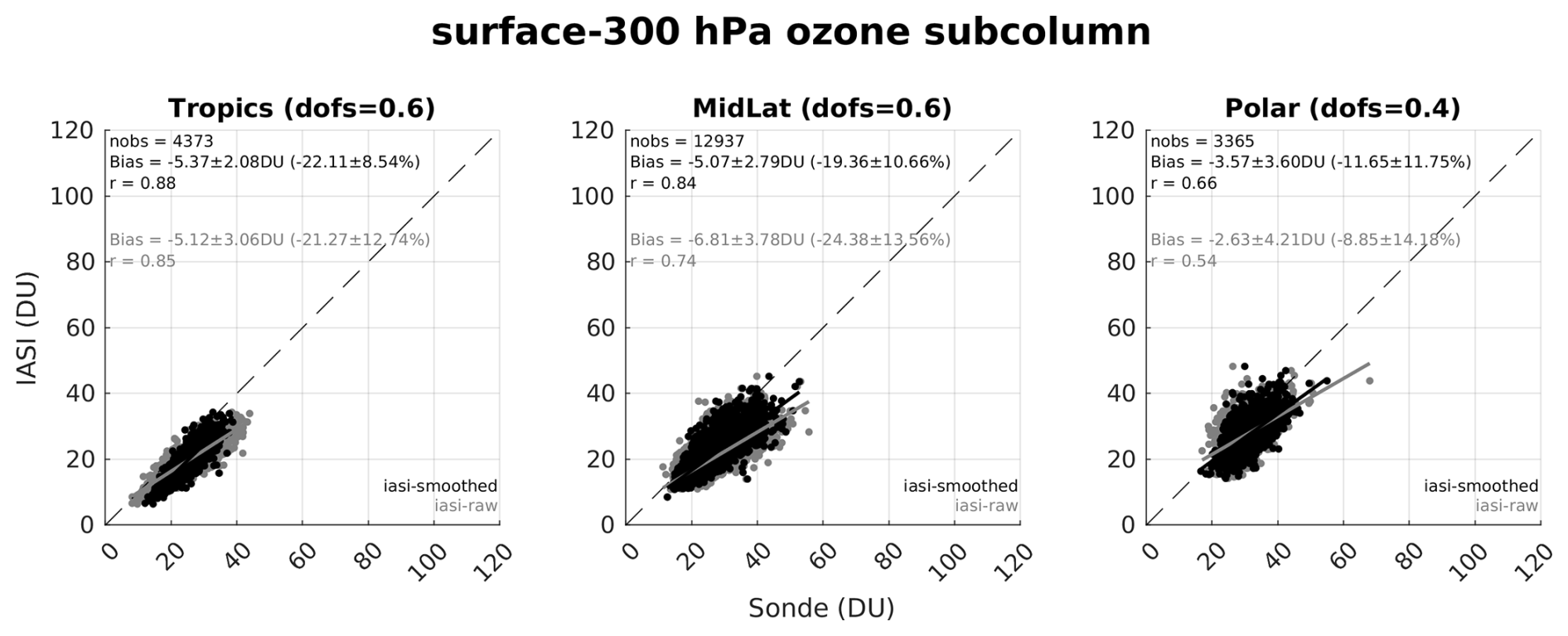
Figure A1 Comparison of IASI with raw (gray) and smoothed (black) sonde surface – 300 hPa ozone subcolumns for the period 2008–2023, shown across three latitude bands: tropics (30° S–30° N), midlatitudes (30–60° North and South) and polar regions (60–90° North and South). The 1:1 line (dashed) and the linear regression lines (black for smoothed, gray for raw) are shown on each scatterplot, along with statistics including the number of collocations, mean bias with standard deviation in both Dobson units (DU) and percent (%), correlation coefficient (r), and the associated mean Degrees of Freedom for Signal (DOFS).

Figure A2 Same as Fig. A1, but for the 300–150 hPa subcolumn.

Figure A3 Same as Fig. A1, but for the 150–25 hPa subcolumn.

Figure A4 Same as Fig. A1, but for the 25–3 hPa subcolumn.

Appendix B: IASI and CrIS a priori data

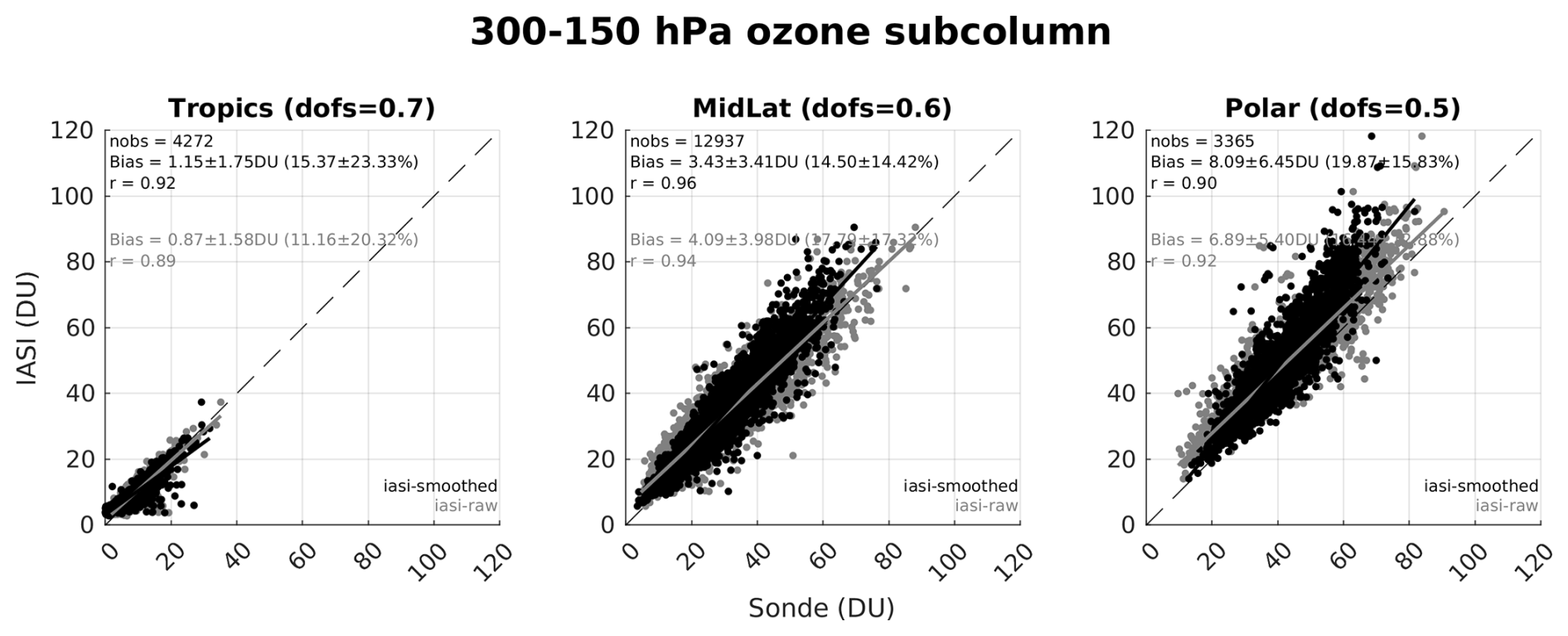
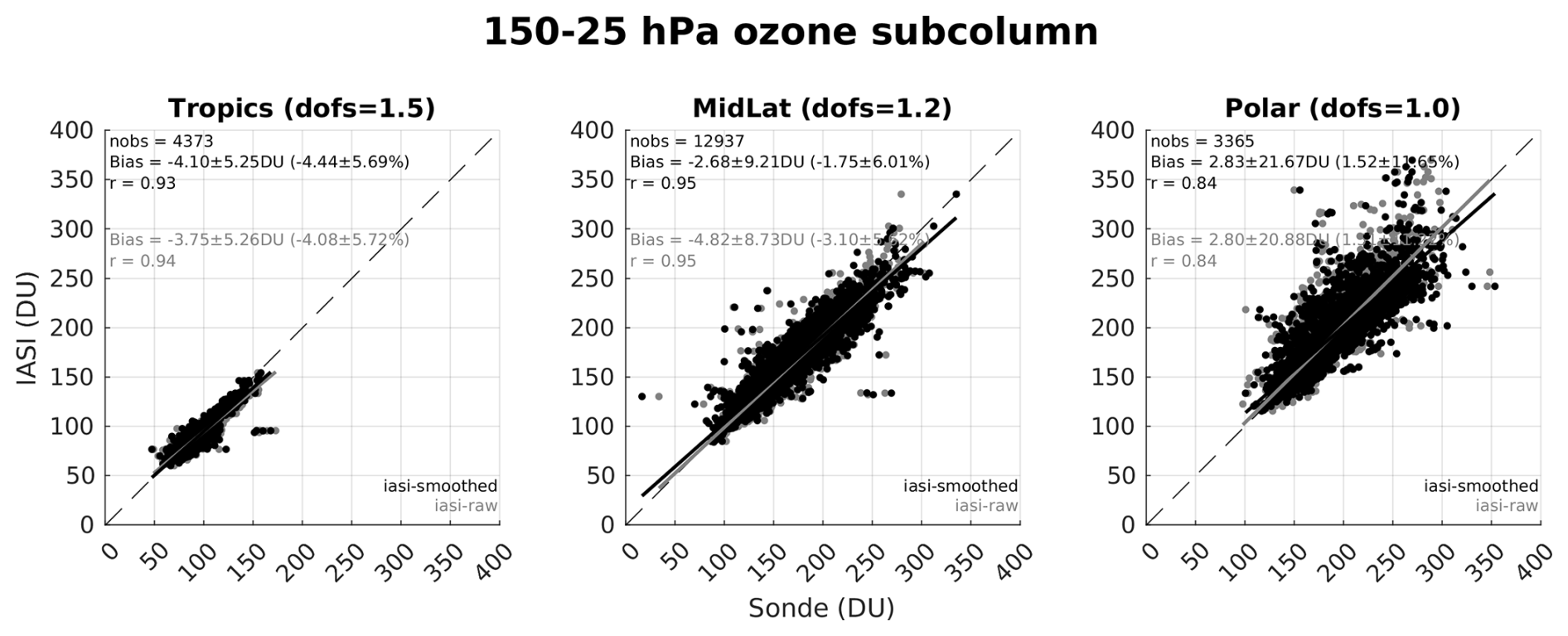
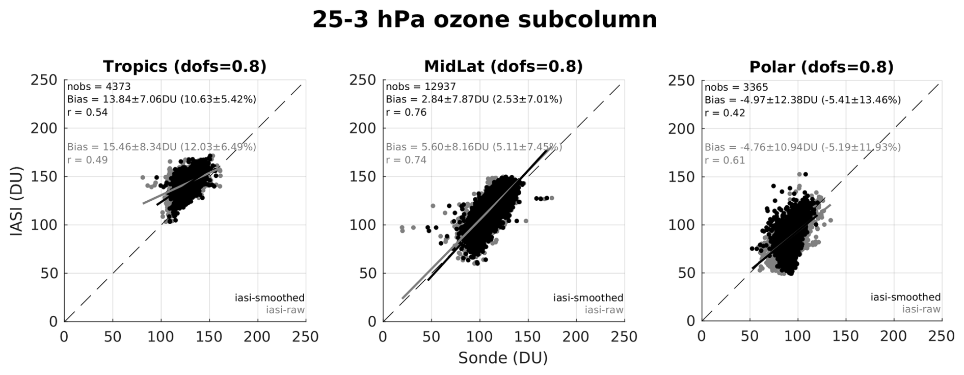
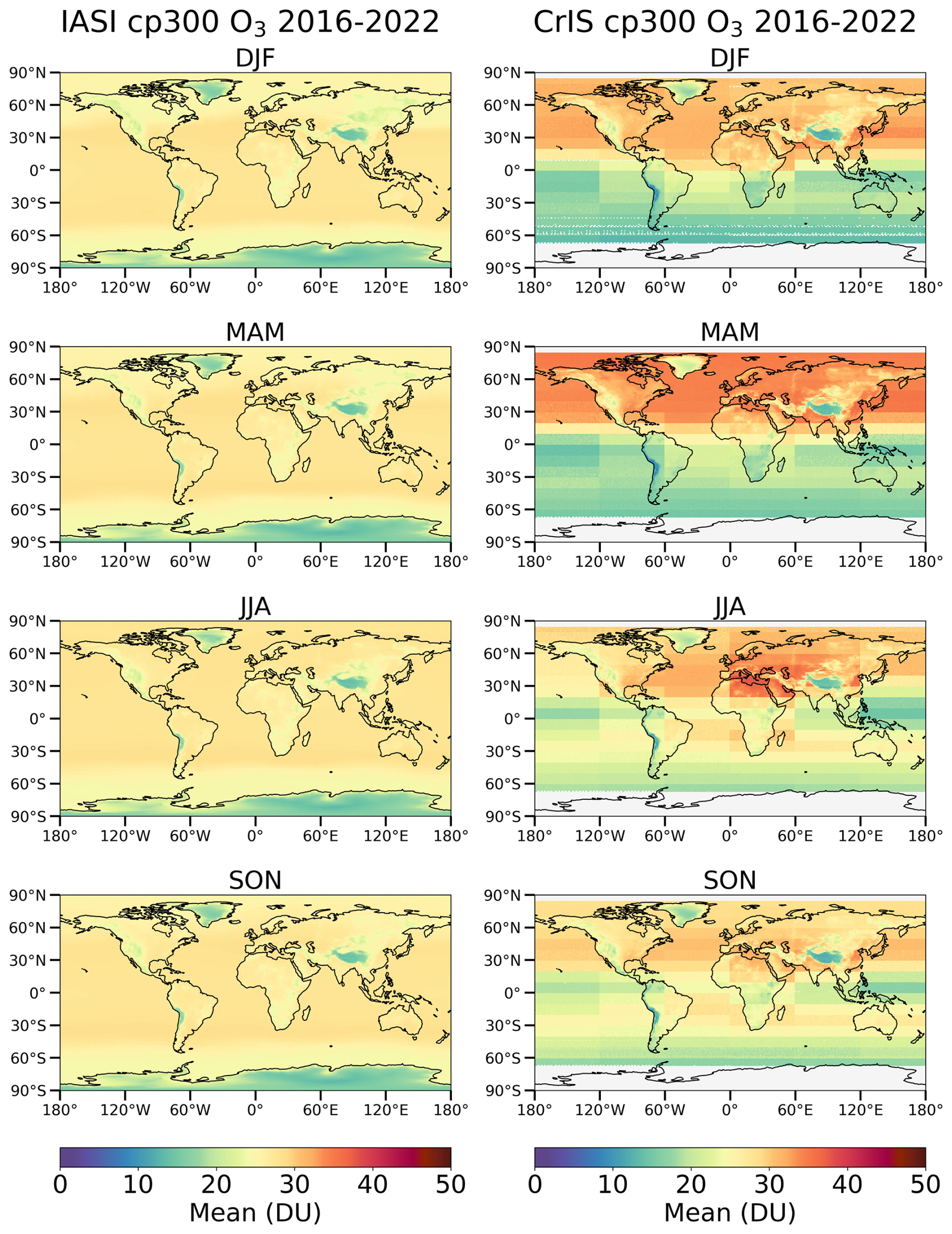
Figure B1 Spatial and seasonal distribution of IASI and CrIS a priori surface–300 hPa ozone column over the period 2016–2022 in Dobson units (DU). The data are averaged on a global grid with a resolution of 1°×1°. The a priori profile for IASI is constant, so there is no seasonal variation, while the a priori data for CrIS varies across seasons.

Appendix C: Tropospheric ozone trends derived from IASI-CDR at the 90th (a) and 95th (b) percentiles

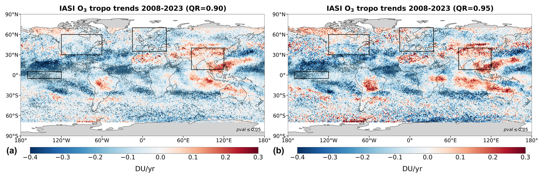
Figure C1 Spatial distribution of tropospheric ozone trends (in DU yr⁻¹) derived from IASI-CDR for the period 2008–2023 at the 90th (a) and 95th (b) percentiles. The tropospheric column is integrated from the surface to the thermal tropopause, as defined by the World Meteorological Organization (WMO, 1957). Dots indicate trends with high to very high certainty (p-value ≦0.05). The black rectangles indicate the boundaries of the regions analyzed in Fig. 13.

Appendix D: Lower and upper tropospheric ozone trends derived from IASI-CDR

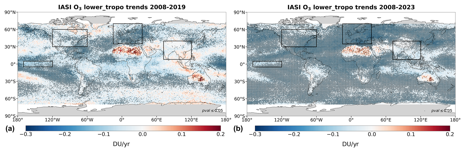
Figure D1 Spatial distribution of lower tropospheric ozone (surface–450 hPa) trends (in DU yr⁻¹) derived from IASI-CDR before the COVID-19 pandemic (2008–2019, a) and including the pandemic (2008–2023, b). Dots indicate trends with high to very high certainty (p-value ≦0.05). The black rectangles indicate the boundaries of the regions analyzed in Fig. 13.

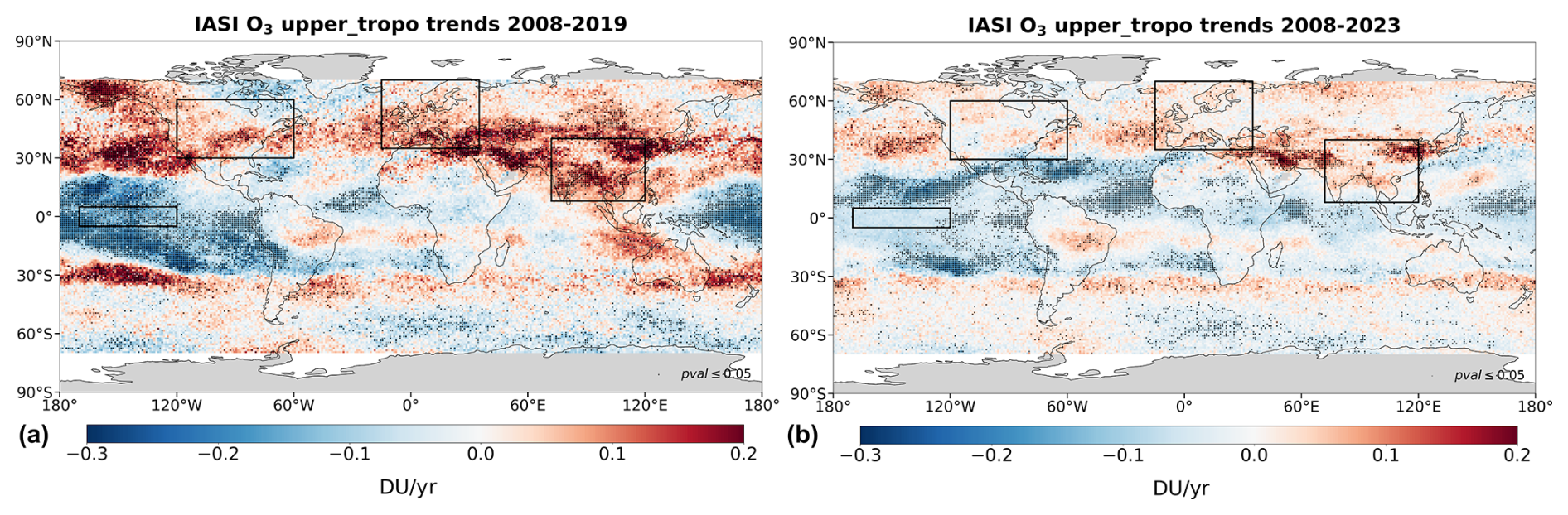
Figure D2 Spatial distribution of upper tropospheric ozone (450 hPa–tropopause) trends (in DU yr⁻¹) derived from IASI-CDR before the COVID-19 pandemic (2008–2019, a) and including the pandemic (2008–2023, b). The tropopause altitude is estimated using the WMO thermal definition. Dots indicate trends with high to very high certainty (p-value $<=\mathrm{0.05}$). The black rectangles indicate the boundaries of the regions analyzed in Fig. 13.