Modeling support for an extensive Δ¹⁴CO₂ flask sample monitoring campaign over Europe to constrain fossil CO₂ emissions

During 2024, an intensive Δ¹⁴CO₂ flask sampling campaign was conducted at 12 sampling stations across Europe as part of the CO2MVS Research on Supplementary Observations (CORSO) project. These Δ¹⁴CO₂ samples, combined with CO₂ atmospheric measurements, are intended to enhance the estimation of fossil CO₂ emissions over Europe through inverse modeling. In this study, we perform a series of Observing System Simulation Experiments (OSSEs) to evaluate the added value of such an intensive campaign as well as the different flask sample selection strategies on estimating fossil fuel emissions. We explore three main selection strategies and compare them against the currently more widely used method of two-week integrated samples: (1) collecting flask samples every 3 d according to a uniform schedule, without applying specific selection criteria; (2) selecting flask samples with high fossil CO₂ content to better isolate anthropogenic signals; and (3) combining fossil CO₂ selection with consideration of nuclear ¹⁴CO₂ contamination to reduce potential biases from nuclear emissions. The results suggest that higher sampling density improves the estimation of fossil CO₂ emissions, particularly during periods of high fossil fuel activity, such as in winter, while integrated sampling remains more effective during summer months when emissions are lower. Increasing the number of flask samples significantly reduces uncertainty and enhances the robustness of inverse modeling results. In addition, selecting samples with a high fossil CO₂ content shows potential for improving the accuracy of emission estimates. The largest reduction in uncertainty is achieved when sample selection actively avoids periods of potential high nuclear ¹⁴CO₂ contamination. This approach helps minimize potential biases, particularly in regions with significant nuclear activity such as France and the UK. These findings highlight the importance of not only increasing sampling frequency but also carefully selecting samples based on their fossil CO₂ and nuclear ¹⁴CO₂ composition to improve the reliability of fossil fuel emission estimates across Europe.

1 Introduction

Inverse modeling has become a key tool for quantifying the anthropogenic contribution to atmospheric CO₂ levels. This approach combines regular CO₂ observations with additional tracers that are sensitive to specific sources and processes. Some of these tracers are measured in situ, such as Δ¹⁴CO₂, CO, and APO (Basu et al., 2020; Wang et al., 2020; Chawner et al., 2024), while others, like XCO₂, are retrieved remotely (Fischer et al., 2017; Chen et al., 2023). These tracers help distinguish fossil fuel emissions from natural biogeochemical fluxes, and their integration into inverse models provides stronger constraints on source attribution. A leading example is radiocarbon (¹⁴C) in atmospheric CO₂. Fossil CO₂ lacks radiocarbon due to its decay over geological timescales (half-life of 5730 years), leading to a measurable reduction in the radiocarbon content of atmospheric Δ¹⁴CO₂ (Levin et al., 2003).

However, in Europe and other industrialized regions, the ability to isolate fossil CO₂ using radiocarbon is complicated by the presence of radiocarbon emissions from nuclear facilities. These emissions can artificially elevate atmospheric Δ¹⁴CO₂ levels, masking the depletion signal caused by fossil CO₂ and potentially leading to biased estimates (Turnbull et al., 2009). For example, Graven and Gruber (2011) showed that in Europe, North America, and East Asia, radiocarbon from nuclear sources can offset around 20 % of the depletion caused by fossil emissions, leading to attribution biases that may exceed those caused by biospheric fluxes in some areas. Vogel et al. (2013), in a local application in Toronto, found that this offset can reach up to 82 % of the total annual fossil CO₂ signal. A sensitivity study by Maier et al. (2023) further showed that uncorrected nuclear emissions could result in a 25 % low bias in ffCO₂ estimates, highlighting the need for robust modeling and informed sample selection strategies.

Data on nuclear facility emissions are generally limited to annual emissions, accessible through databases such as the European Commission RAdioactive Discharges Database (RADD) (https://europa.eu/radd/index.dox, last access: 17 June 2025) or derived from energy production data from the Power Reactor Information System (PRIS) (https://pris.iaea.org/PRIS/home.aspx, last access: September 2025). These datasets often lack the high temporal resolution necessary to identify the possible effect of large emission events in radiocarbon samples. Studies such as those by Graven and Gruber (2011) and Zazzeri et al. (2018) provide essential emission factors and data, but also highlight the high-resolution data availability gap we just mentioned. Strict data protection policies and security measures further compound the challenge of obtaining high-resolution time series data from nuclear facilities. Few studies have directly measured and reported emissions from nuclear facilities (Akata et al., 2013; Varga et al., 2020; Lehmuskoski et al., 2021) at higher temporal resolutions, such as daily or weekly. Vogel et al. (2013) for instance, found significant deviations in interannual timescales of nuclear emissions compared to emission factors reported by Graven and Gruber (2011), but a better agreement with the long-term average observed for reactors in their study area. Most research examining the impact of nuclear emissions on ffCO₂ estimation is conducted in the vicinity of nuclear facilities, which allows sampling of winds directly coming from these facilities, reducing the need for high-resolution emission time series (Vogel et al., 2013; Kuderer et al., 2018). Consequently, the broader implications of nuclear emissions and their temporal variations on regional and continental scales remain less explored and understood, as evidenced in the study by Vogel et al. (2013). This localized focus limits our understanding of the impact of nuclear facility emissions on ffCO₂ estimations on a continental scale, such as for Europe. In addition, in inverse modeling approaches that include both CO₂ and Δ¹⁴CO₂, the emissions from nuclear facilities are not optimized, leading to potential inaccuracies. Research by Bozhinova et al. (2014); Graven and Gruber (2011); Turnbull et al. (2011); Zazzeri et al. (2018) demonstrates this gap, suggesting the need for more sophisticated modeling and sampling approaches to integrate nuclear emissions accurately into atmospheric inversion techniques.

In Europe, the Integrated Carbon Observation System (ICOS) Atmosphere network continuously measures CO₂ together with other greenhouse gases (GHG) at 38 stations in Europe. Additional atmospheric tracers, including isotopic tracers such as ¹³C and radiocarbon (¹⁴C), are measured in periodic flask samples at 17 of these ICOS stations (see Fig. 1). Most of the stations are located in remote locations, where measurements are taken from tall towers of at least 100 m above ground level, on mountain tops, and on coastal sites (in the last two, measurements are usually taken a few meters above ground level). The objective of the network is to provide measurements intended to represent large areas, capturing signals from sources and sinks occurring even hundreds of kilometers away. Currently, radiocarbon is measured mainly in two-weekly integrated flask samples, at the highest sampling height available at each station (red and yellow dots in Fig. 1). Since 2015, an increasing number of ICOS stations have been collecting 1 h flask samples regularly. Of the approximately 100 flask samples taken per station per year as quality control of continuous measurements and for the analysis of other tracers and isotopes, around 25 are selected for Δ¹⁴CO₂ analysis to support the estimation of ffCO₂. Levin et al. (2020) designed a strategy to select flask samples that mainly captured large events of fossil fuel CO₂ emissions for their posterior analysis of Δ¹⁴CO₂. They suggested defining a threshold for the mixing ratio of ffCO₂ and for the enhancement of CO (CO is a co-emmitted species from fossil fuel burning) relative to the background mixing ratio at the time the flask sample is taken. This can be determined by near-real-time (NRT) atmospheric transport simulations (for ffCO₂ and ffCO) or by using continuous observations of CO at the station.

As part of the CO2MVS Research on Supplementary Observations (CORSO) project (https://www.corso-project.eu/, last access: September 2025) funded by the Horizon Europe program of the European Commission, an intensive sampling campaign of Δ¹⁴CO₂ was carried out in 2024. In this project, flask samples are taken approximately every three days, completely dedicated to the analysis of Δ¹⁴CO₂ at 10 of the current ICOS sampling stations around Sweden, Germany, the Netherlands, France and the Czech Republic, complemented by two additional stations in Poland (Białystok) and England (Heathfield), and three background stations that take 2-weekly integrated samples in Ireland (Mace Head), Spain (Izaña), and Canada (Alert). Given the high analytical costs, labor intensity, and limited laboratory capacity associated with Δ¹⁴CO₂ measurements, implementing a sample selection strategy is essential to maximize the information gained while minimizing resource use. Identifying the most informative sampling times and locations helps optimize observational coverage, enabling more cost-effective network design without compromising the accuracy of fossil CO₂ estimates.

In this paper, we assess how different sample selection strategies, combining intensive flask sampling with regular integrated sampling, can improve fossil CO₂ emission estimates at subregional and subannual scales. We use the multi-tracer-enabled version of the Lund University Modular Inversion Algorithm (LUMIA) system (Gómez-Ortiz et al., 2025) to perform a series of perfect transport OSSEs. The study aims to address three key research questions: (1) What is the added value of intensive Δ¹⁴CO₂ sampling compared to the current sampling done in ICOS? (2) Is there a benefit in selecting Δ¹⁴CO₂ flask samples based on their fossil contribution to improve fossil CO₂ emissions estimates? (3) Does further selection of flask samples based on nuclear contamination provide additional benefits when estimating fossil CO₂ emissions?

To address these questions, we calculate a series of synthetic observations by performing a forward simulation of the transport model with a set of assumed true fluxes. We then apply different flask sample selection strategies based on fossil CO₂ content, and nuclear ¹⁴CO₂ contamination. These synthetic observations are subsequently inverted using LUMIA to estimate fossil CO₂ emissions, allowing us to quantify differences in bias and uncertainty associated with each selection approach. The framework and strategies presented here were developed prior to and during the early stages of the 2024 campaign to support its design and implementation. They enable a comprehensive evaluation of how increasing flask sampling frequency and accounting for both fossil and nuclear signals can improve the estimation of fossil fuel emissions at subregional and subannual scales, ultimately providing insights to optimize future greenhouse gas monitoring efforts.

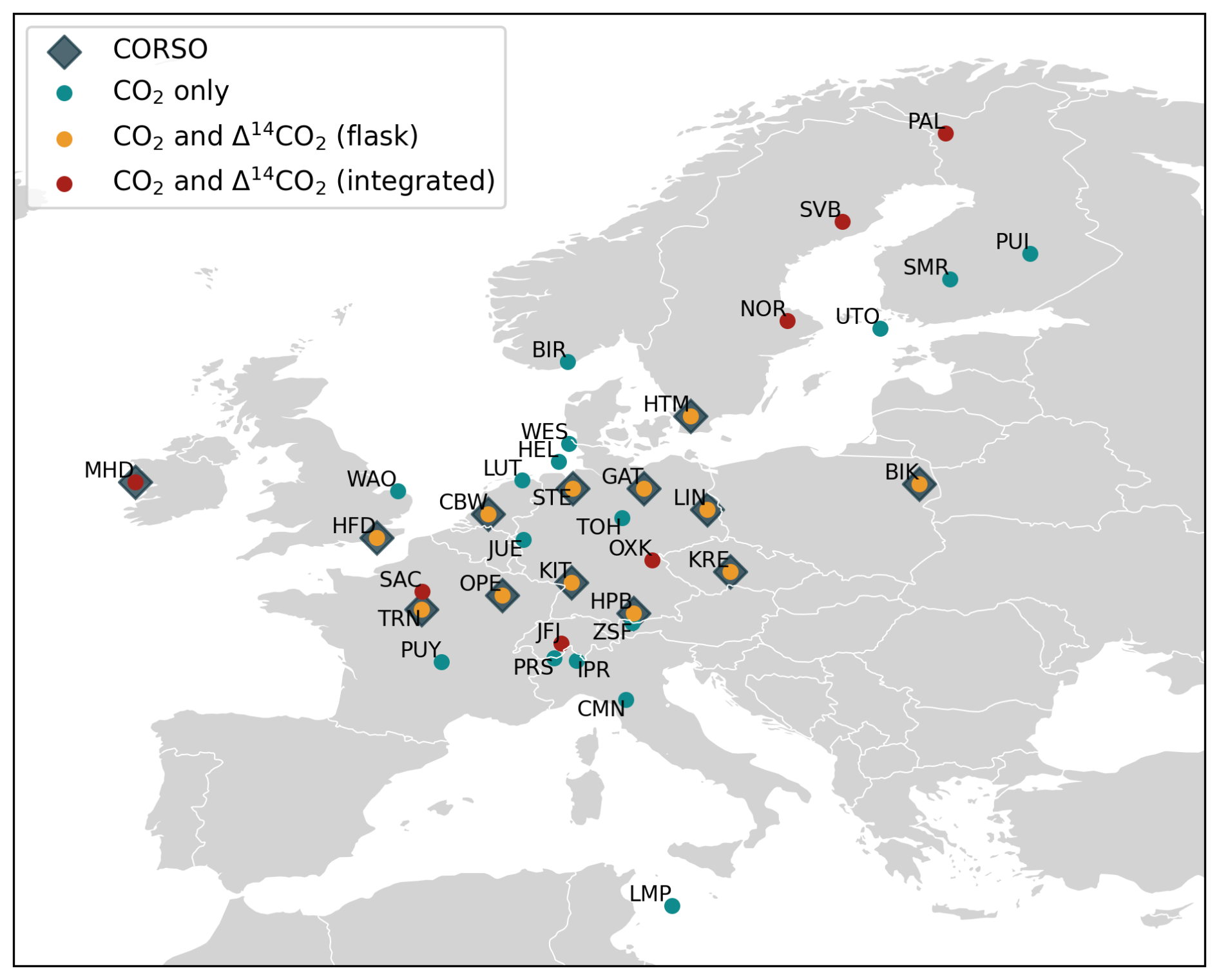
Figure 1 Sampling stations selected for this study and their identification according to the measured tracers and their participation in the CORSO project (dark blue diamonds). Green dots represent the stations where only CO₂ is measured, yellow dots where additionally Δ¹⁴CO₂ is measured in 1 h flasks and red dots where Δ¹⁴CO₂ is measured in approximately 2-weekly integrated samples.

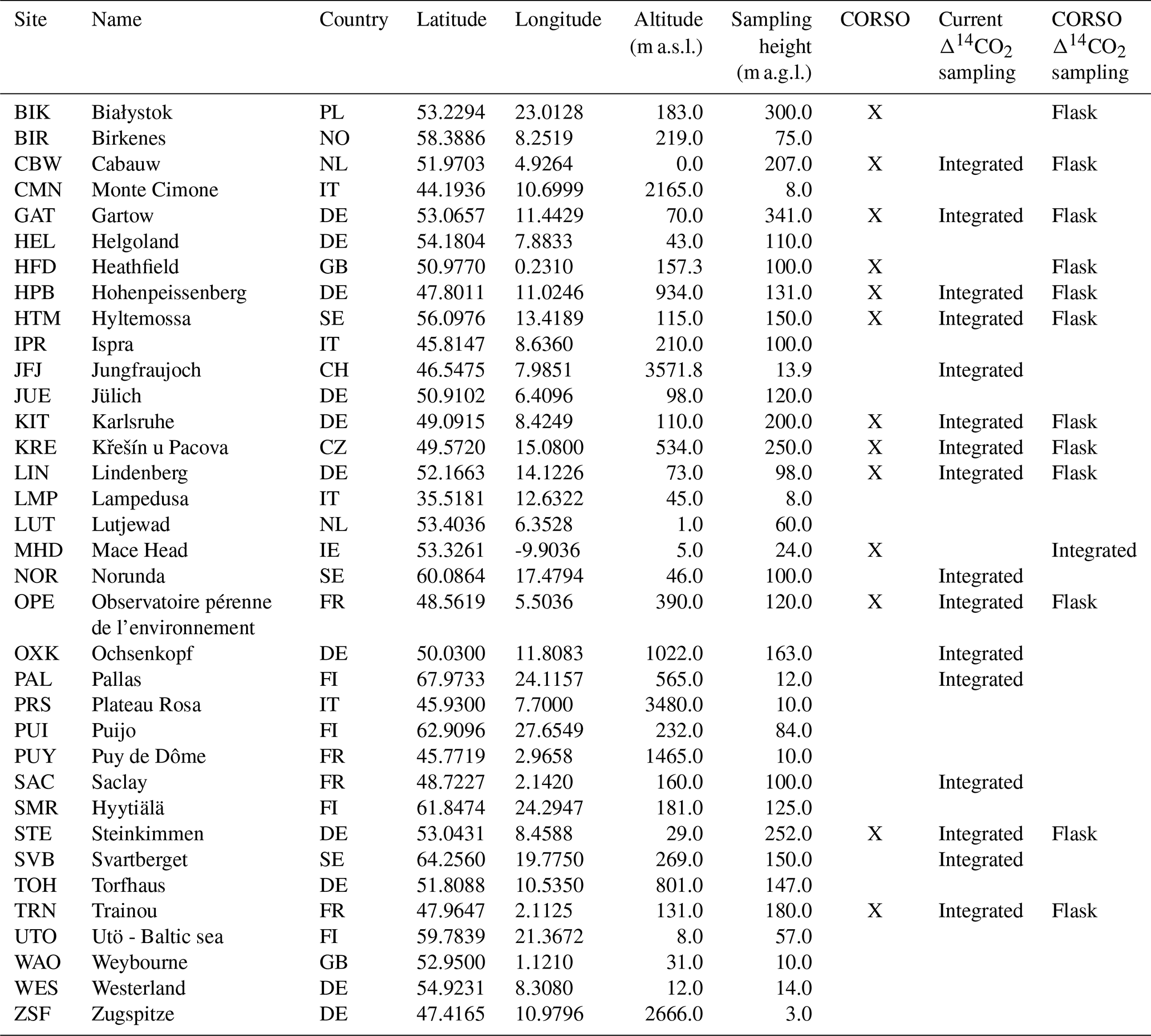
Table 1 Sampling stations included in this study and Δ¹⁴CO₂ sampling type according to the current status and the CORSO project.

2 The LUMIA framework

We use the multi-tracer-enabled version of the Lund University Modular Inversion Algorithm (LUMIA) system (Gómez-Ortiz et al., 2025) to perform a series of perfect transport OSSEs covering Europe in a regional domain ranging from 15° W, 33° N to 35° E, 73° N, as shown in Fig. 1, similar to previous regional European inverse modeling studies (Monteil et al., 2020; Thompson et al., 2020). In this case, perfect transport means that we use the same transport model to produce the synthetic observations and to perform the atmospheric inversions, as well as the same background for the synthetic observations and the modeled mixing ratios.

LUMIA is an inversion framework originally designed for regional CO₂ inversions in Europe. The framework was later extended to perform simultaneous inversions of CO₂ and Δ¹⁴CO₂ to estimate fossil CO₂ emissions over Europe (Gómez-Ortiz et al., 2025), which we use in this study with minor modifications detailed in this section. Since the initial release of LUMIA, it has incorporated the two-step atmospheric inversion scheme proposed by Rödenbeck et al. (2009), as thoroughly explained by Monteil and Scholze (2021). In this approach, for each observation (either CO₂ or Δ¹⁴CO₂), the modeled mixing ratio y^m is described as the total of the contributions of the “foreground” y^f (mixing ratios due to fluxes directly related with y^m by the model, limited spatially by the domain and temporally by the length of the simulation) and the “background” y^b (i.e., any additional contribution not captured by the foreground fluxes, including external sources or preexisting atmospheric mixing ratios):

$$\begin{array}{}\text{(1)}& {\mathit{y}}^{\text{m}}={\mathit{y}}^{\text{b}}+{\mathit{y}}^{\text{f}}\end{array}$$

which can be expanded for each tracer (CO₂ and Δ¹⁴CO₂) as:

$$\begin{array}{}\text{(2a)}& {\displaystyle }{\mathit{y}}_{{\text{CO}}_{\mathrm{2}}}^{\text{m}}={\mathit{y}}_{{\text{CO}}_{\mathrm{2}}}^{\text{b}}+{\mathit{y}}_{\text{ff}}^{\text{f}}+{\mathit{y}}_{\text{bio}}^{\text{f}}+{\mathit{y}}_{\text{oce}}^{\text{f}}\text{(2b)}& {\displaystyle }\begin{array}{rl}{\mathit{y}}_{\text{C}{\mathrm{\Delta }}^{\mathrm{14}}\text{C}}^{\text{m}}& =\underset{\text{background}}{\underbrace{{\mathit{y}}_{\text{C}{\mathrm{\Delta }}^{\mathrm{14}}\text{C}}^{\text{b}}+{\mathit{y}}_{\text{cosmo}}^{\text{b}}}}\\ & +\underset{\text{foreground}}{\underbrace{{\mathit{y}}_{\mathrm{\Delta }\text{ff}}^{\text{f}}+{\mathit{y}}_{\mathrm{\Delta }\text{bio}}^{\text{f}}+{\mathit{y}}_{\mathrm{\Delta }\text{oce}}^{\text{f}}+{\mathit{y}}_{\text{biodis}}^{\text{f}}+{\mathit{y}}_{\text{ocedis}}^{\text{f}}+{\mathit{y}}_{\text{nuc}}^{\text{f}}}}\end{array}\end{array}$$

where ${\mathit{y}}_{{\text{CO}}_{\mathrm{2}}}^{\text{m}}$ is the modeled CO₂ mixing ratio and ${\mathit{y}}_{{\text{CO}}_{\mathrm{2}}}^{\text{b}}$ is the background CO₂ mixing ratio. On the right-hand side of Eq. (2a), ${\mathit{y}}_{\text{ff}}^{\text{f}}$ is the mixing ratio within the domain due to fossil CO₂ (F_ff), ${\mathit{y}}_{\text{bio}}^{\text{f}}$ the mixing ratio due to the net exchange of CO₂ between the atmosphere and terrestrial ecosystems (Net Ecosystem Exchange, NEE, hereafter biosphere flux, F_bio) , and ${\mathit{y}}_{\text{oce}}^{\text{f}}$ the mixing ratio due to the net exchange of CO₂ between the atmosphere and oceans (F_oce).

All terms in Eq. (2b) are in units of CO₂×Δ¹⁴CO₂ (e.g. ppm ‰) or CΔ¹⁴C for simplification, since the values in ‰ are not additive (see Basu et al., 2016; Gómez-Ortiz et al., 2025, for additional details). In this equation, ${\mathit{y}}_{\text{C}{\mathrm{\Delta }}^{\mathrm{14}}\text{C}}^{\text{m}}$ and ${\mathit{y}}_{\text{C}{\mathrm{\Delta }}^{\mathrm{14}}\text{C}}^{\text{b}}$ are the modeled and background CΔ¹⁴C mixing ratios, respectively. ${\mathit{y}}_{\text{cosmo}}^{\text{b}}$ is the CΔ¹⁴C mixing ratio due to the cosmogenic production of radiocarbon in the stratosphere (F_cosmo). ${\mathit{y}}_{\text{cosmo}}^{\text{b}}$ is accounted in the background (${\mathit{y}}_{\text{C}{\mathrm{\Delta }}^{\mathrm{14}}\text{C}}^{\text{b}}$), since LUMIA was designed to assimilate only surface fluxes. Furthermore, on a regional scale, sampling sites are considered to be similarly influenced by ¹⁴C-enriched stratospheric air and its influence on tropospheric radiocarbon can be neglected (Maier et al., 2023; Lingenfelter, 1963). A significant influence from cosmogenic radiocarbon production can be expected in samples collected near the lower stratosphere (above 6 km) (Turnbull et al., 2009) which is not the case for any stations in this study (see Fig. 1).

The first foreground term in Eq. (2b), ${\mathit{y}}_{\mathrm{\Delta }\text{ff}}^{\text{f}}$, represents the reduction in atmospheric Δ¹⁴CO₂ due to the addition of fossil CO₂, which is devoid of radiocarbon. This dilution effect is modeled by transporting a tracer, ${\mathit{y}}_{\mathrm{\Delta }\text{ff}}^{\text{f}}$, assigned a Δ¹⁴CO₂ value of −1000 ‰, representing fossil CO₂ with no radiocarbon content relative to the atmospheric standard. The next terms, ${\mathit{y}}_{\mathrm{\Delta }\text{bio}}^{\text{f}}$ and ${\mathit{y}}_{\mathrm{\Delta }\text{oce}}^{\text{f}}$ represent the net exchange from the atmosphere with the biosphere and the ocean, respectively. The contribution of these exchanges is modeled by transporting the biosphere and ocean fluxes multiplied by the isotope signature of the current atmosphere. ${\mathit{y}}_{\text{biodis}}^{\text{f}}$ and ${\mathit{y}}_{\text{ocedis}}^{\text{f}}$ are the contributions due to isotopic disequilibrium.

The carbon exchanged between the biosphere, ocean, and atmosphere has an isotopic signature that can differ from that of the current atmosphere. In the terrestrial biosphere, carbon released through heterotrophic respiration may be enriched in ¹⁴C, reflecting the elevated atmospheric radiocarbon levels that followed nuclear weapons testing in the mid-20th century (Levin and Kromer, 2004; Graven et al., 2012). This enrichment introduces a positive isotopic disequilibrium between biospheric fluxes and the present-day atmosphere. In contrast, the ocean can release ¹⁴C-depleted carbon, especially from older subsurface waters that have been isolated from atmospheric exchange for decades, allowing radioactive decay to reduce their radiocarbon content below atmospheric levels (Sweeney et al., 2007; Graven et al., 2012). These opposing disequilibrium fluxes contribute to regional and seasonal variability in atmospheric Δ¹⁴CO₂.

The last term, ${\mathit{y}}_{\text{nuc}}^{\text{f}}$, represents the contribution due to the radiocarbon emissions generated by nuclear activities (F_nuc), mainly from nuclear power plants and spent fuel reprocessing facilities. The contribution of past nuclear weapons testing is now considered negligible due to its significant decline over recent decades (Kutschera, 2022), and is therefore not included.

Following the original the original implementation of LUMIA (Monteil and Scholze, 2021), here we use the global TM5 model (Huijnen et al., 2010) to calculate the background mixing ratios (y^b) and the Lagrangian FLEXPART model (Pisso et al., 2019) to perform the regional transport (y^f) and the inversions. In the following sections, we explain further the implementation of the models.

2.1 Background composition from TM5

The background refers to the CO₂ mixing ratio and Δ¹⁴CO₂ isotopic signature of the atmosphere at the spatial and temporal boundaries of the domain. This can be a combination of emissions transported by large-scale atmospheric circulation, regional transport from outside the domain, and air masses reentering the domain (Rödenbeck et al., 2009). In this study, we use the implementation of the background mixing ratio calculation in TM5-4DVar developed by Monteil and Scholze (2021) based on the methodology proposed by Rödenbeck et al. (2009), integrated with the implementation of TM5-4DVar to include CO₂ or Δ¹⁴CO₂ developed by Basu et al. (2016) (https://sourceforge.net/p/tm5/cy3_4dvar/ci/default/tree/proj/tracer/radio_co2/, last access: August 2024). Here, we model the background mixing ratio using global optimized fluxes and an initial condition from Basu et al. (2020) for 2010. These fluxes are in a horizontal resolution of 3° × 2° (25 hybrid sigma-pressure vertical levels for F_cosmo), and variable time resolutions for the individual fluxes: 1 h for F_ff, 3 h for F_bio and F_oce, 1 month for F_biodis and F_ocedis, and 1 year for F_nuc and F_cosmo. The simulation is driven by meteorological fields from the European Centre for Medium-Range Weather Forecasts (ECMWF) ERA5 reanalysis project (Hersbach et al., 2020).

Here, we describe a extension of the original setup by Monteil and Scholze (2021) to include cosmogenic production in the background term ${\mathit{y}}_{\text{C}{\mathrm{\Delta }}^{\mathrm{14}}\text{C}}^{\text{b}}$ (see Sect. 2, Eq. 2b):

The background component ${\mathit{y}}_{\text{t}}^{\text{b}}$, with t indicating the tracers CO₂ and CΔ¹⁴C, is calculated as follows:

1. We perform a global forward run with TM5 to calculate the mixing ratio field ${\mathit{y}}_{\text{t}}^{\text{TM5}}$, which include contributions from both inside and outside the regional domain.

2. We then run a modified version of TM5 in which all fluxes and mixing ratios are set to zero outside the regional domain at every time step. This produces a field ${\mathit{y}}_{\text{t}}^{\text{f, TM5}}$, which reflects only the contribution from fluxes inside the regional domain. In this step, the cosmogenic production flux F_cosmo is set to zero globally in order to keep it as part of the background in the next step.

3. The background mixing ratios are then calculated as: ${\mathit{y}}_{\text{t}}^{\text{b}}={\mathit{y}}_{\text{t}}^{\text{TM5}}-{\mathit{y}}_{\text{t}}^{\text{f, TM5}}$.

2.2 Regional transport (FLEXPART)

Following the methodology described in Monteil and Scholze (2021) and Gómez-Ortiz et al. (2025), our regional transport model (i.e. the operator to calculate y^f in Eqs. 1 and 2) is composed of a series of pre-computed footprints with FLEXPART (Pisso et al., 2019) driven by ERA5 reanalysis data for 2018 at a spatio-temporal resolution of 0.25° × 0.25° and 1 h, using the Python code developed to run and post-process the footprints to be used in LUMIA (https://github.com/lumia-dev/runflex, last access: July 2025). We compute two types of footprints: (i) instant (or flask) footprints to simulate continuous CO₂ and CO observations, and (ii) integrated footprints to simulate Δ¹⁴CO₂ integrated observations (see Sect. 3.5 and 3.3).

We compute instant footprints from the observation time and 14 d back in time releasing 10 000 particles per simulation (Monteil and Scholze, 2021), and we use the same footprint to model CO₂, CO, and Δ¹⁴CO₂ at the corresponding observation time and sampling station. These footprints are computed for a passive air tracer, i.e. without any atmospheric chemistry reactions. Therefore, for CO we only evaluate the regional contributions (Levin et al., 2020) without accounting for the background and reactions with other atmospheric components. For the integrated footprints, we set a fixed integration time of 2 weeks (14 d), distribute 10 000 FLEXPART particles per hour over this integration period, and then simulate 14 d backward from the integration start time (Gómez-Ortiz et al., 2025).

2.3 The inverse modeling approach

LUMIA follows an implementation of the variational approach (4D-Var). This approach seeks to iteratively minimize the mismatch between the model output and observations δ_y by optimizing the control vector x. The optimization process is guided by a cost function, J(x), defined as:

$$\begin{array}{}\text{(3)}& \begin{array}{rl}J\left(\mathit{x}\right)& ={\displaystyle \frac{\mathrm{1}}{\mathrm{2}}}{\left(\mathit{x}-{\mathit{x}}^{\text{b}}\right)}^T{\mathbf{\text{B}}}^{-\mathrm{1}}\left(\mathit{x}-{\mathit{x}}^{\text{b}}\right)\\ & +{\displaystyle \frac{\mathrm{1}}{\mathrm{2}}}{\left(\mathbf{\text{H}}\mathit{x}-{\mathit{\delta }}_{\mathit{y}}\right)}^T{\mathbf{\text{R}}}^{-\mathrm{1}}\left(\mathbf{\text{H}}\mathit{x}-{\mathit{\delta }}_{\mathit{y}}\right)\end{array}\end{array}$$

In this equation, x^b represents the prior estimate of the control vector, B is the prior uncertainty covariance matrix, R is the observational uncertainty covariance matrix, and H is the Jacobian of the observation operator H, which includes the transport model (i.e., pre-computed footprints) and other components needed to express y as a function of x, such as flux aggregation and disaggregation, and the incorporation of boundary conditions.

The control vector x contains the set of parameters adjustable by the inversion, which are offsets to the fossil and biosphere CO₂ fluxes we aim to estimate. We solve for clusters aggregated in time and space. These are defined based on the sensitivity of the observation network to emissions from different regions: areas with high observational coverage, such as those upwind of sampling stations, are optimized at full spatial resolution (0.5° × 0.5°), while regions with lower sensitivity are grouped into coarser clusters (e.g., 5° × 3.5°) (Gómez-Ortiz et al., 2025).

The prior error covariance matrix (B) is constructed in three steps. First, the variances are determined to represent the assumed spatio-temporal uncertainties of the fluxes. Next, covariances are calculated based on assumed spatial and temporal correlations, incorporating the distance between grid clusters and the time difference between flux intervals. Finally, the entire matrix is scaled using a uniform factor to match category-specific annual uncertainty values. The formulas used for fossil CO₂ emissions differ from those used for other fluxes to account for better-known emission locations and to avoid artificially low uncertainties due to flux compensations (Gómez-Ortiz et al., 2025).

The observation uncertainty matrix (R) includes both measurement uncertainties and model representation uncertainties, which account for the model's inability to perfectly simulate observations even with accurate fluxes. Ideally, the diagonal of R holds the total uncertainty for each observation, while the off-diagonals represent error correlations between observations. However, since these correlations are hard to quantify, common practice is to set these error correlations (off-diagonal elements) to zero. The observation uncertainty can then be provided as a simplified observation error vector (Monteil and Scholze, 2021).

The iterative procedure works by adjusting x to minimize the cost function J(x), which represents the mismatch between the model and the observations weighted by their respective uncertainties. The optimal solution is achieved when the gradient, ∇_xJ approaches zero, indicating that a local minimum of the cost function has been reached. This approach ensures that the final estimate of x provides the best possible fit to the synthetic observational data while taking into account the uncertainties in both the prior information and the observations (Rayner et al., 2019).

3 Experimental design

In this paper, we focus on the implementation of perfect transport OSSEs. We calculate a series of synthetic observations, using a set of assumed “true” fluxes (F^t), by performing a forward run of our transport model. Afterwards, using a set of “prior” fluxes, we can evaluate how well the inversion framework performs in recovering the assumed “true” fluxes. In this section, we describe the flux products used as true and prior fluxes (Sect. 3.1), the calculation of the synthetic observations (Sect. 3.3), the model setup (i.e., the information needed to construct the matrices B and R and the control vector x) (Sect. 3.4), the selection criteria of the synthetic Δ¹⁴CO₂ flask samples (Sect. 3.5), and the design of the OSSEs (Sect. 3.6).

3.1 True, prior and prescribed fluxes

The assumed true fluxes, denoted as F^t, are used to generate synthetic observations through a forward run of our transport model. For the global transport simulation, we use the posterior fluxes from Basu et al. (2020) (see Sect. 2.1). For the regional transport, all fluxes have a resolution of 0.5° × 0.5° and 1 h in the domain shown in Fig. 1.

We use as true fossil CO₂ flux (${\mathit{F}}_{\text{ff}}^{\text{t}}$) a product (Koch and Gerbig, 2023) for 2018 based on the Emission Database for Global Atmospheric Research (EDGAR) version 4.3.2 emission product (Janssens-Maenhout et al., 2019) following temporal variations based on MACC-TNO Denier van der Gon et al. (2011) and with temporal extrapolations and disaggregation using the COFFEE approach (Steinbach et al., 2011). We use a fossil CO flux product based on the same methodology described for ${\mathit{F}}_{\text{ff}}^{\text{t}}$. This product is later used to estimate the CO enhancement from fossil fuel combustion, used as a criterion for selecting the Δ¹⁴CO₂ flask samples.

As true biosphere fluxes (${\mathit{F}}_{\text{bio}}^{\text{t}}$), we use a simulation for 2018 from the LPJ-GUESS vegetation model (Wu, 2023; Smith et al., 2014). For true ocean fluxes (${\mathit{F}}_{\text{oce}}^{\text{t}}$), we use the Jena CarboScope oc_v2020 product, which is based on the SOCAT dataset of pCO2 observations (van der Woude et al., 2022; Rödenbeck et al., 2022, 2013). As true terrestrial and oceanic isotopic disequilibrium fluxes (${\mathit{F}}_{\text{biodis}}^{\text{t}}$ and ${\mathit{F}}_{\text{ocedis}}^{\text{t}}$), we use the optimized fluxes from Basu et al. (2020), regridded to match the spatial and temporal resolution of the regional transport model. Both disequilibrium fluxes are prescribed in the experiments, and hence they are not optimized. This decision is due to the high uncertainty derived from optimizing F_biodis, and the low influence of F_oce and F_ocedis in the study domain, as shown in our earlier work (Gómez-Ortiz et al., 2025). The emission products from nuclear facilities are described in detail in Sect. 3.2.

As prior fluxes, we use the Open-source Data Inventory for Anthropogenic CO₂ (ODIAC) (Oda et al., 2018) for 2018 (Oda and Maksyutov, 2020) to represent prior fossil CO₂ emissions (F_ff). For prior biosphere emissions (F_bio), we use fluxes simulated by the Vegetation Photosynthesis and Respiration Model (VPRM) (Mahadevan et al., 2008; Thompson et al., 2020) for the year 2018 (Gerbig and Koch, 2021).

3.2 Radiocarbon emissions from nuclear facilities (F_nuc)

Nuclear ¹⁴CO₂ fluxes (F_nuc) are generally prescribed in inverse modeling studies due to the high uncertainty derived from the lack of information on temporal variability. For this reason, we produced two sets of nuclear fluxes: one with a temporal variability to be used as the true flux (${\mathit{F}}_{\text{nuc}}^{\text{t}}$), and the second one with the emissions evenly distributed throughout the year as is usual for this flux category (Basu et al., 2016, 2020; Gómez-Ortiz et al., 2025). Both flux products are based on the data described in Maier et al. (2023) and Storm et al. (2024). Therefore, they share the same annual budget and spatial distribution, which is defined using the location of nuclear facilities and aggregated over a 0.5° × 0.5° grid.

For the temporal distribution of ${\mathit{F}}_{\text{nuc}}^{\text{t}}$, we use the weekly temporal profiles reported by Varga et al. (2020) for the Paks Nuclear Power Plant (NPP) in Hungary and the monthly profiles reported by Akata et al. (2013) for the Rokkasho Spent Fuel Reprocessing Plant (SFR) in Japan. Both studies reported at least three years of temporal profiles. Therefore, we assign the temporal profile by randomly selecting a time span corresponding to a year starting from a random date and then assigning it to the corresponding type of nuclear facility (NPP or SFR). We did this because we did not find any evident seasonality in the temporal profiles of these two studies, and, in addition, such temporal profiles can vary between different types of nuclear reactors. With this temporal distribution, we want to add extra variability to the nuclear contribution to atmospheric Δ¹⁴CO₂ and study its impact when using the prescribed flat-year nuclear emissions to estimate fossil CO₂ emissions. However, we are aware of the differences among the types of nuclear facilities and how this can affect the temporal profile. For the prescribed flux, we incorporate a flat-year nuclear emission product. This allows the inversion to follow a traditional setup while still accounting for imperfect representation of nuclear emissions.

3.3 Synthetic observations

We calculate hourly mixing ratios for each sampling station. For the flask (Δ¹⁴CO₂) samples and the instant (CO₂) observations, the background is the model output at each observation time. For the integrated Δ¹⁴CO₂ samples, the background is calculated as the average of the mixing ratios from the start date of sampling to the end of the integration period (14 d in this study).

Using the instant and integrated footprints , we perform a forward run of the regional model with the true fluxes (see Sect. 3.1) to generate time series of CO₂, CO, and Δ¹⁴CO₂. The CO flux product is based on the same methodology as the fossil CO₂ flux and is used to simulate CO mixing ratios for sample selection, following the approach of Levin et al. (2020), where elevated CO deviations from background are used as a proxy for enhanced fossil CO₂ signals.

As a final step, we add random noise to the synthetic CO₂ and Δ¹⁴CO₂ observations by drawing from a normal distribution with mean zero and a standard deviation equal to the assumed observational uncertainty. This perturbation is added to each observation to mitigate the assumption of a perfect transport model.

We select the CO₂ synthetic observations for the times of day when the model is expected to perform well, as typically done in real atmospheric inversions. This corresponds to 11:00–15:00 local time (LT) for sampling sites below 1000 $\mathrm{m}\mathrm{a}.\mathrm{s}.\mathrm{l}.$, and 22:00–02:00 LT for mountaintop stations, when the boundary layer is likely below the sampling intake and free tropospheric air is sampled (Monteil and Scholze, 2021; Gómez-Ortiz et al., 2025).

3.4 Inversion setup

In all experiments, we optimize weekly fossil and biospheric CO2 fluxes (Fff and F_bio). The control vector x is composed of clusters of 2500 grid points and weekly offsets for each flux category. Uncertainties are first defined at the native resolution of the prior fluxes (e.g. 0.5° × 0.5°, hourly) and then aggregated to match the resolution of the control vector. This ensures that regions and time periods with larger fluxes are assigned proportionally larger uncertainties, while still allowing all clusters to be adjusted by the inversion.

For fossil fuel emissions, we distribute uncertainty across grid cells using the ratio $\log \left(\text{Daily total}\right)/\text{Daily total}$. This gives relatively more weight to low-emission regions, which often carry higher relative uncertainty, and prevents unrealistically low uncertainty values in high-emission areas. For biospheric fluxes, uncertainty is distributed in proportion to the square root of the sum of the absolute hourly fluxes within each aggregation window. This avoids underestimating uncertainty in regions or periods where net biospheric fluxes are small due to compensation between photosynthesis and respiration.

The overall prior uncertainty across the domain is set to 0.21 Pg C yr⁻¹ for fossil emissions (30 % of the prior annual budget) and 0.37 Pg C yr⁻¹ for biosphere fluxes (25 % of the absolute prior annual budget). These values are consistent with observed differences between fossil and biosphere model products (e.g. EDGAR vs. ODIAC, LPJ-GUESS vs. VPRM).

The spatial and temporal error structure in the prior covariance matrix B is defined using an exponential temporal correlation of one month for both fluxes, and a Gaussian spatial correlation length of 200 km for fossil fluxes and 500 km for biospheric fluxes. These correlation lengths reflect the structure of uncertainty in emission inventories and ecosystem processes, and are consistent with previous inversion studies in Europe (Wang et al., 2018; Monteil and Scholze, 2021; Thompson et al., 2020).

Observation uncertainties in R are defined as follows: for CO₂, we assign a prior error equal to the standard deviation of model-simulated concentrations within a ±3.5 d window around each observation. For Δ¹⁴CO₂, we assume a constant error of 0.9 ppm CΔ¹⁴C, equivalent to 2.15±0.05 ‰.

3.5 Synthetic Δ¹⁴CO₂ flask sample selection

We define three criteria to guide the selection of Δ¹⁴CO₂ flask samples in the OSSEs: (1) midday sampling at 13:00 LT every third day, (2) selection of high fossil CO₂ events, and (3) avoidance of periods with potentially high nuclear emissions. These correspond to the three strategies described earlier but are detailed here with their specific operational implementation. Sampling at midday ensures strong atmospheric mixing, reducing model transport errors and providing stable, low-variability conditions for accurate quality control. Events of high fossil CO₂ are identified using the simulated mixing ratios of fossil CO₂ and fossil CO, the latter serving as a reliable tracer due to its co-emission during combustion and lack of biological sources. While these are simulated values in the OSSE framework, in real-world applications, total CO₂ and total CO measurements are used in near-real time. Fossil CO₂ is then inferred from observed CO enhancements relative to a background, together with known emission ratios, as described by Levin et al. (2020). Avoiding potentially high nuclear emissions is crucial to prevent masking the fossil fuel signal with nuclear ¹⁴CO₂ emissions (Maier et al., 2023; Graven and Gruber, 2011).

For the Δ¹⁴CO₂ flask sample selection, we follow the same thresholds for fossil CO₂ (≥4 ppm) and fossil CO (≥40 ppb) (hereafter ffCO₂ and ffCO, respectively) as proposed by Levin et al. (2020) to capture events of high fossil CO₂ emissions. Additionally, we introduce a new threshold for nuclear CΔ¹⁴C of ≤1 ppm CΔ¹⁴C to avoid capturing events of potentially high nuclear Δ¹⁴CO₂ contamination. This value is based on forward runs using both nuclear emission products (with and without a temporal profile). Because LUMIA calculates the individual contribution of each flux category in Eq. (2) to the modeled tracer fields, these estimates are used directly to apply the sample selection strategies.

At sites not directly influenced by nuclear emissions, such as Białystok (BIK; see Fig. 1 and Table 1), this threshold represents 87 % of the synthetic observations at 13:00 local time for the year 2018. In contrast, at sites with high nuclear impact, such as Karlsruhe (KIT) in Germany, it represents 41 % of the synthetic observations (see Fig. 2). This estimate is based on simulations for 2018, when nearby nuclear facilities like Philippsburg 2 (shut down at the end of 2019) were still active. However, conditions during the CORSO campaign may differ significantly due to the shutdown of all German nuclear power plants in April 2023.

During the CORSO sampling campaign, approximately 120 flask samples (10 per month) are selected at each station for Δ¹⁴CO₂ analysis. Maintaining a consistent number of samples per station and distributing them as evenly as possible throughout the year is desirable to reduce seasonal bias. However, this distribution is not always achievable when applying strict sampling criteria, particularly in regions or periods with frequent nuclear contamination or low fossil signals. Therefore, we prioritize synthetic samples that meet the selection thresholds in each OSSE and complete the 10-per-month target with additional samples that closely match the criteria.

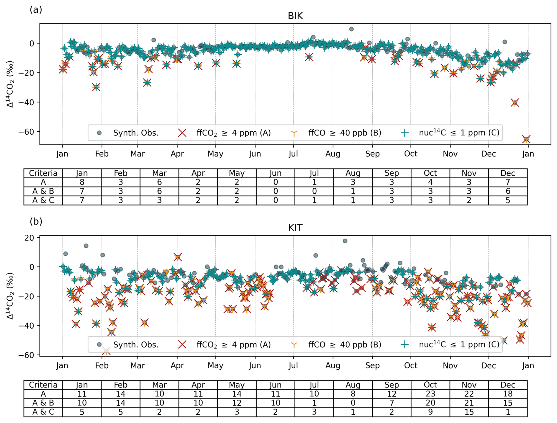
Figure 2 Synthetic Δ¹⁴CO₂ flask samples at (a) Białystok (BIK) and (b) Karlsruhe (KIT), two of the 12 sampling sites selected for the intensive sampling campaign during the CORSO project. The time series for the remaining sampling sites can be found in Appendix A1. The tables below each figure show the number of synthetic observations per month that meet the ffCO₂ threshold (red cross), the ffCO₂ and ffCO (yellow tri) thresholds, and the ffCO₂ and nuc¹⁴C (green cross) thresholds.

3.6 Observing System Simulation Experiments (OSSEs)

In the following sections, we describe the experiments. We summarize the setup of the experiments and their criteria in Table 2. As part of the evaluation of the experiments, we calculate the posterior uncertainty of each OSSE with a Monte Carlo ensemble of 25 members. Note that small differences in the monthly prior uncertainties across figures are due to the limited size (25 members) of each Monte Carlo ensemble, despite the same annual prescribed uncertainty being applied across all regions and experiments.

3.6.1 Base case scenario (BASE)

In the first inversion, BASE, we replicate the current setup of the ICOS network using synthetic Δ¹⁴CO₂ integrated samples and synthetic CO₂ observations. In this experiment, we use all stations in Fig. 1 (except MHD, HFD and BIK) and integrated samples according to the column “Current Δ¹⁴CO₂ sampling” in Table 1 (yellow and red dots in Fig. 1). CO₂ observations are used at all stations during periods of the day when the atmospheric transport model is expected to perform best: midday at lowland and coastal sites, and midnight at mountaintop sites.

3.6.2 Including Δ¹⁴CO₂ flask samples (CORSO)

The selection of flask samples represents many logistic and operational challenges. The simulations and data analysis to determine if a sample meets the selection criteria are often conducted weeks after the sample has been taken. As a result, more than 10 samples need to be collected each month, which requires sufficient flasks, storage, and transport capacity. Therefore, we will begin by evaluating the use of synthetic Δ¹⁴CO₂ flask samples in the simplest form: taking a sample every 3 d at 13:00 local time, regardless of its composition. This experiment also works as a base case for the use of Δ¹⁴CO₂ flask samples. The selection in this and the following experiments is carried out in the sampling sites marked with yellow dots in Fig. 1. This is the basic approach to sampling selection in the CORSO project when it is not possible to perform near-real-time simulations to estimate the fossil or nuclear contribution of the Δ¹⁴CO₂ flask samples.

3.6.3 Applying fossil fuel-related thresholds (ffCO₂ and ffCO)

We apply the fossil fuel-related thresholds (ffCO₂ and ffCO) using a forward simulation with prior fluxes to approximate near-real-time conditions. Based on the resulting mixing ratios, we select the synthetic observations that meet the defined criteria. These thresholds are not always satisfied, particularly in summer when fossil emissions are lower and most stations fail to meet the minimum values. This seasonal pattern is consistent with the decline in fossil fuel activity during warmer months, as also noted by Levin et al. (2020). Figure 2 illustrates the variability in threshold fulfillment across sites.

In months in which one of the thresholds or a combination of them is not met, we still need to select the 10 synthetic observations that best fit the experimental conditions. The first experiment including the thresholds is CORSO_ffCO2, where we select synthetic observations at 13:00 LT with a fossil CO₂ component greater than or equal to 4 ppm (see Fig. 2). Generally, we select the 10 synthetic observations per month with the highest fossil CO₂ component. The second experiment is CORSO_ffCO2_ffCO (criteria A & B in Fig. 2). In this experiment, when neither threshold is met, we select the best combination with the highest values of ffCO₂ and ffCO.

3.6.4 Evaluating the impact of nuclear emissions (nuc¹⁴C)

In the final set of experiments, we aim to estimate the contribution of nuclear emissions to the posterior uncertainty. In a real-world application, sample selection would rely on the sensitivity of the observations to nuclear emissions (i.e., whether the upstream winds pass over a nuclear facility and coincide with a period of radiocarbon release). Although there is substantial uncertainty in the estimated magnitude of nuclear contamination, we maintain reasonable confidence in the modeled spatial and temporal patterns.

To replicate a real world scenario, we select a set of observations with low nuclear influence (CORSO_ffCO2_nuc14C) while ensuring a high ffCO₂ composition. We use a forward run of the prior nuclear fluxes, assumed to be evenly distributed throughout the year, to estimate the nuclear CΔ¹⁴C component. Since the combination of the ffCO₂ and nuc¹⁴C thresholds (criteria A and C in Fig. 2) is not always satisfied, we apply the following selection procedure in the CORSO_ffCO2_nuc14C experiment:

1. We first select the observations that meet both the ffCO₂ and nuc¹⁴C thresholds.

2. For each site, year, and month, we then select the top 10 observations with the lowest nuclear influence from this subset.

3. If fewer than 10 such observations are available, we fill the remaining slots with observations that meet the ffCO₂ threshold and have moderate nuclear influence (1–2 ppm CΔ¹⁴C).

4. If this is still insufficient, we complete the sample by selecting observations that meet only the nuclear threshold, prioritizing those with the highest fossil CO₂ influence.

We compare this experiment against CORSO_ffCO2, in which we do not consider the nuclear contamination. For each set of observations (CORSO_ffCO2 and CORSO_ffCO2_nuc14C), we perform two Monte Carlo ensembles. In the first, we conduct a standard ensemble in which both the control vector and the observations are perturbed according to the prescribed uncertainties. In the second ensemble, we additionally include uncertainty from nuclear emissions by modifying the observation error as follows: we perturb the true nuclear emissions using an uncertainty equal to the annual nuclear budget (0.62 Pg CΔ¹⁴C, 100 %), and recalculate the synthetic observations. We assign 100 % uncertainty to the nuclear emissions due to the lack of information on their temporal distribution, following Maier et al. (2023). After this, we perform the Monte Carlo ensemble in the same way as the first. The difference between the two ensembles for each observation set represents the contribution of nuclear emissions to the posterior uncertainty.

Table 2 Summary of the OSSEs performed in this study.

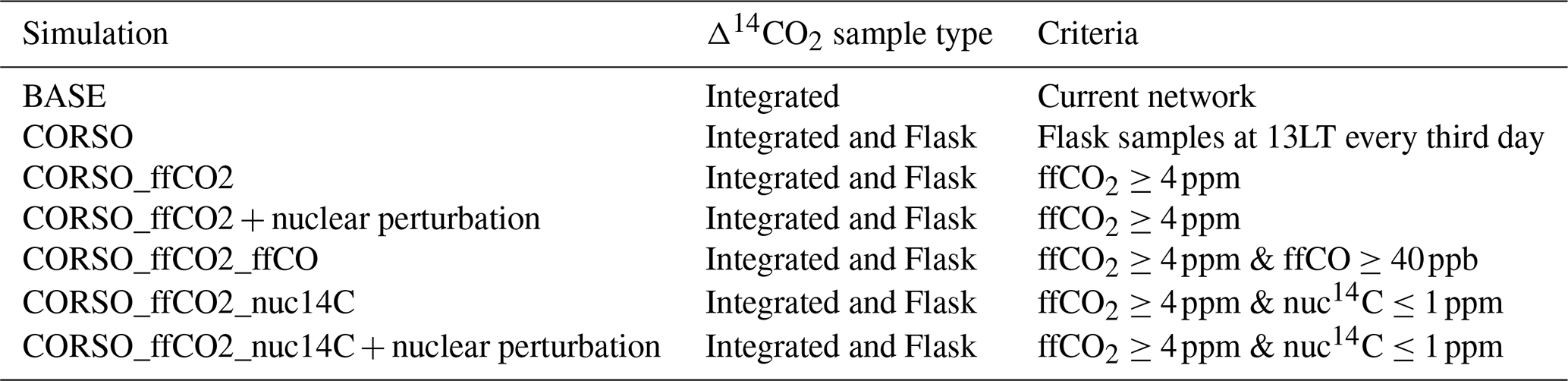
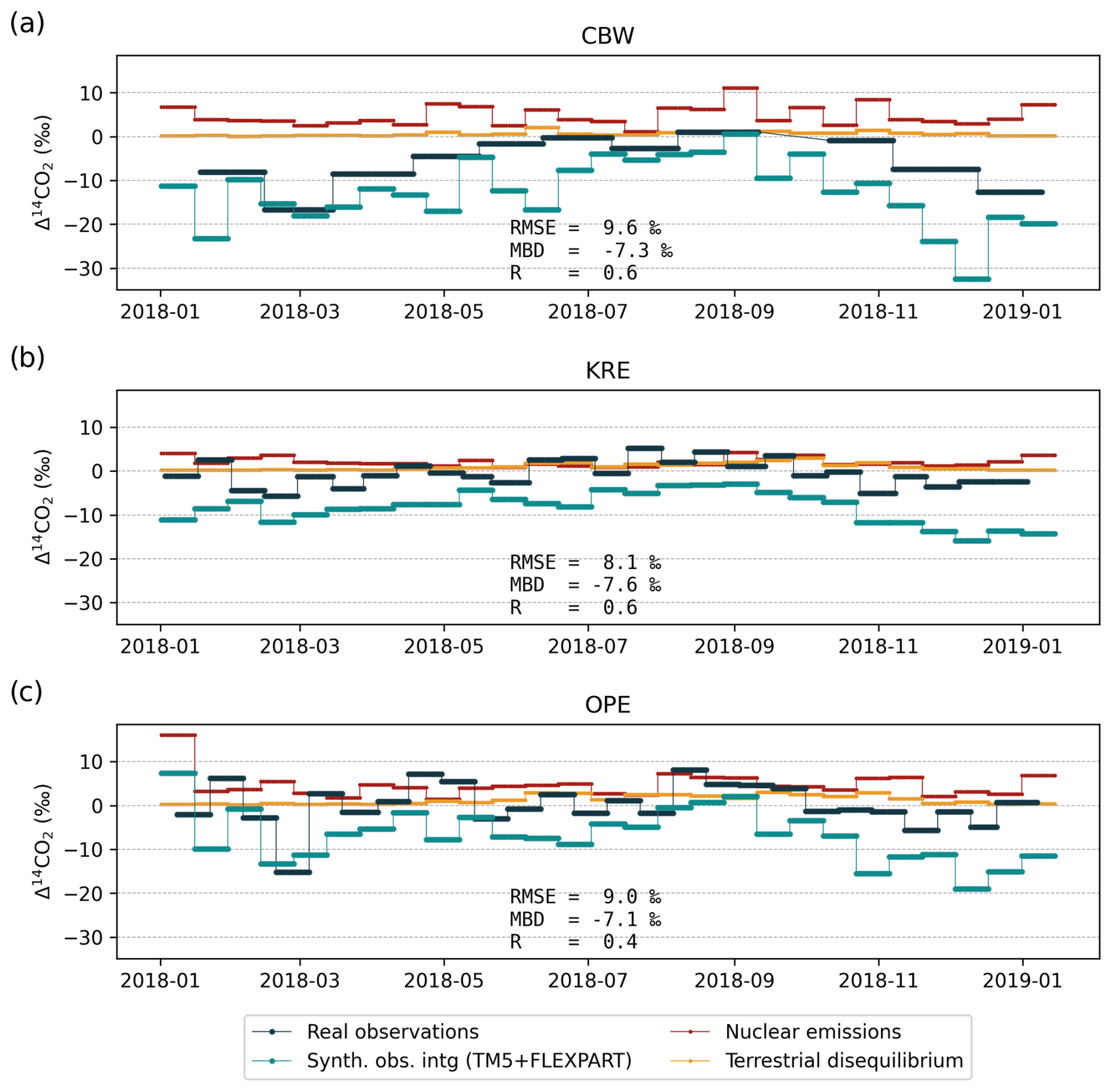
Figure 3 Comparison of the available real Δ¹⁴CO₂ integrated samples (black) (ICOS RI et al., 2024) with the modeled synthetic observations (teal) at (a) CBW, (b) KRE and (c) OPE, three of the sampling sites selected for the intensive CORSO flask campaign. The nuclear (red) and terrestrial disequilibrium (yellow) components of the synthetic observations are also shown for comparison. Gaps in panel (a) reflect periods of missing integrated observations. At CBW, the integration period was approximately one month during 2018, whereas it was around 14 d at the other stations. Synthetic observations were modeled to match fixed 14 d integration periods across sites.

4 Results

4.1 Characterization of the sampling sites in terms of Δ¹⁴CO₂

We start by analyzing and comparing the real Δ¹⁴CO₂ integrated samples (ICOS RI et al., 2024) with the synthetic observations at the sites selected for the intensive Δ¹⁴CO₂ flask sample campaign (Fig. 3 and Appendix A2). Real observations show pronounced seasonal but also episodic fluctuations in Δ¹⁴CO₂, such as low values during February and March in CBW (−16.64 ‰), OPE (−15.14 ‰), and KRE (−5.75 ‰) (black line; see Fig. 3), which also coincide with the reduction in the modeled synthetic observations (between −7.6 ‰ in CBW and −5.1 ‰ in KRE, teal line) and can be associated with the typically high fossil emissions during winter. In contrast, elevated values are observed in January and February at KRE (2.56 ‰) and OPE (6.25 ‰). These high values may be primarily driven by nuclear emission enrichment, as indicated by the simulated nuclear component (red line; see Fig. 3), which shows contributions of up to 7 ‰ at KRE and OPE during this period. During the growing season, when heterotrophic respiration is more active, elevated values could also be influenced by terrestrial isotopic disequilibrium, as reflected in the simulated component ranging from 1 ‰ to 4 ‰.

Although the synthetic observations are calculated with non-optimized fluxes, we find certain reproducibility of the seasonal patterns at sites such as CBW where we have the best agreement between the real and synthetic observations with the highest correlation coefficient (R) and lowest mean bias deviation (MBE) (see Fig. 3), and KRE and SAC (Fig. A2) in which the synthetic observations mostly underestimate the real observations (negative MBD). Also, at some sampling stations such as JFJ and PAL, the synthetic observations do not capture the variability shown by the real observations, which is reflected in high root mean square error values (RMSE, see Fig. A2).

4.2 OSSEs

We evaluate the retrieval of fossil CO₂ emissions by comparing the assumed true values (from EDGAR) with the prior estimates (from ODIAC) and the posterior estimates from each experiment. The analysis focuses on bias and uncertainty reduction, calculated as follows

$$\begin{array}{}\text{(4a)}& {\displaystyle }\text{Bias reduction}=\left(\mathrm{1}-{\displaystyle \frac{|\text{Posterior}-\text{Truth}|}{|\text{Prior}-\text{Truth}|}}\right)\times \mathrm{100}\text{(4b)}& {\displaystyle }\mathrm{\text{Uncertainty reduction}}=\left(\mathrm{1}-{\displaystyle \frac{\text{Posterior uncertainty}}{\text{Prior uncertainty}}}\right)\times \mathrm{100}\end{array}$$

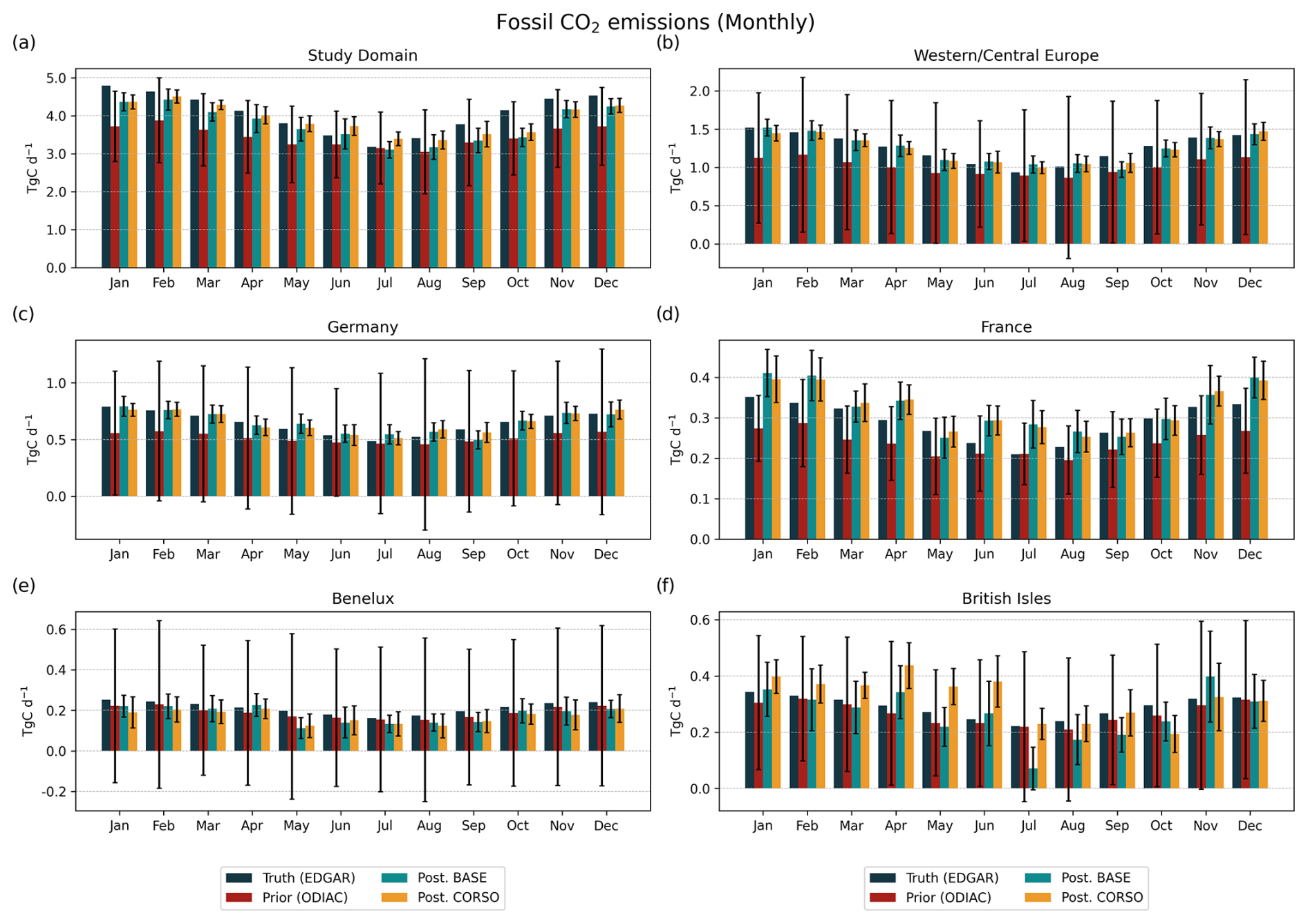
Figure 4 Monthly fossil CO₂ truth (black), prior (red), and posterior fluxes from the BASE (teal) and CORSO (yellow) experiments for (a) the study domain and 5 sub-regions: (b) Western/Central Europe, (c) Germany, (d) France, (e) Benelux, and (f) British Isles. Vertical error bars indicate the associated ±1σ uncertainties from a Monte Carlo ensemble of 25 members. The prior uncertainty is defined independently of the inversion, while posterior uncertainties reflect the constraints imposed by the observations in each experiment.

4.2.1 Impact of adding Δ¹⁴CO₂ flask samples

Here, we compare the BASE and CORSO experiments. A summary of the maximum and minimum bias and uncertainty values, their respective months, and the corresponding posterior reductions is provided in Table 3. In the study domain (Fig. 4a), the true emissions display a clear seasonal pattern, with higher values in winter and lower values in summer, reaching a maximum of approximately 4.8 Tg C d⁻¹ in January and a minimum of about 3.1 Tg C d⁻¹ in July. The prior (ODIAC) underestimates the true emissions throughout the year, particularly in winter months, with a January bias of nearly 30 %. In contrast, the posterior estimates from the BASE and CORSO experiments show improved agreement with the truth. The CORSO experiment generally achieves larger reductions in bias, especially during spring and autumn. However, in June and July, CORSO slightly overestimates emissions, whereas the BASE experiment provides a closer match to the true values. Prior uncertainty ranges from approximately 50 % in winter to over 70 % in summer. Both posterior experiments substantially reduce this uncertainty, with CORSO showing slightly stronger reductions, between 71 % and 87 % across the year.

Western/Central Europe (WCE) and Germany, where around 30 % and 16 % of the total emissions occur, respectively, have similar results in relative terms. Both regions have a larger prior bias during winter, with the largest biases occurring in January (35 % for WCE and 42 % for Germany). In contrast, they exhibit a lower bias in summer, with a minimum in July (5 % for WCE and 4 % for Germany). The posterior emissions of both experiments overestimate the monthly budgets during summer, from June to August in WCE and from May to August in Germany. However, the CORSO experiment shows values closer to the truth in this season. Outside of the summer season, the BASE experiment demonstrates a larger bias reduction in WCE, whereas the CORSO experiment shows a larger bias reduction in Germany. The prior uncertainties in both regions exceed 100 % but are consistently reduced by more than 90 % by the CORSO experiment in both WCE and Germany, and by more than 80 % by the BASE experiment. Nevertheless, from May to September the absolute posterior uncertainty of both experiments in both regions is larger than their respective absolute prior bias.

France, the Benelux region and the British Isles have similar monthly budgets, typically between 0.2 and 0.4 Tg C d⁻¹, and prior biases similar to the other regions (ranging from 0 % to 31 %). However, the performance of the posterior estimates is more mixed across these regions. In France, both BASE and CORSO improve the prior estimate in early months (e.g. January–April), but during summer and autumn, especially July and November, both experiments overestimate emissions, with CORSO showing a stronger deviation from the truth. A similar pattern is observed in Benelux, where uncertainty reductions are substantial (80 %–90 %), but posterior fluxes do not consistently reduce bias and sometimes worsen the agreement (e.g. in July and September). The British Isles exhibit the largest discrepancies: in several months (notably July, October, and November), CORSO notably overestimates emissions, and even BASE deviates from the truth. This highlights that, despite strong uncertainty reductions, the posterior estimates do not always align better with the true values, particularly in regions with smaller source magnitudes or more limited observational constraints.

Overall, both BASE and CORSO experiments lead to substantial improvements over the prior by reducing bias and uncertainty in most regions. However, the differences between the two are not consistent across space and time. CORSO generally achieves greater reductions in uncertainty and improves performance in some areas, such as the core domain and Germany. In contrast, it tends to overestimate emissions in regions like France, Benelux, and the British Isles during summer and autumn. These results reflect the sensitivity of the inversion to the choice of observation sampling strategy. In the following section, we evaluate whether further selecting flask samples based on their fossil CO₂ content can improve the results.

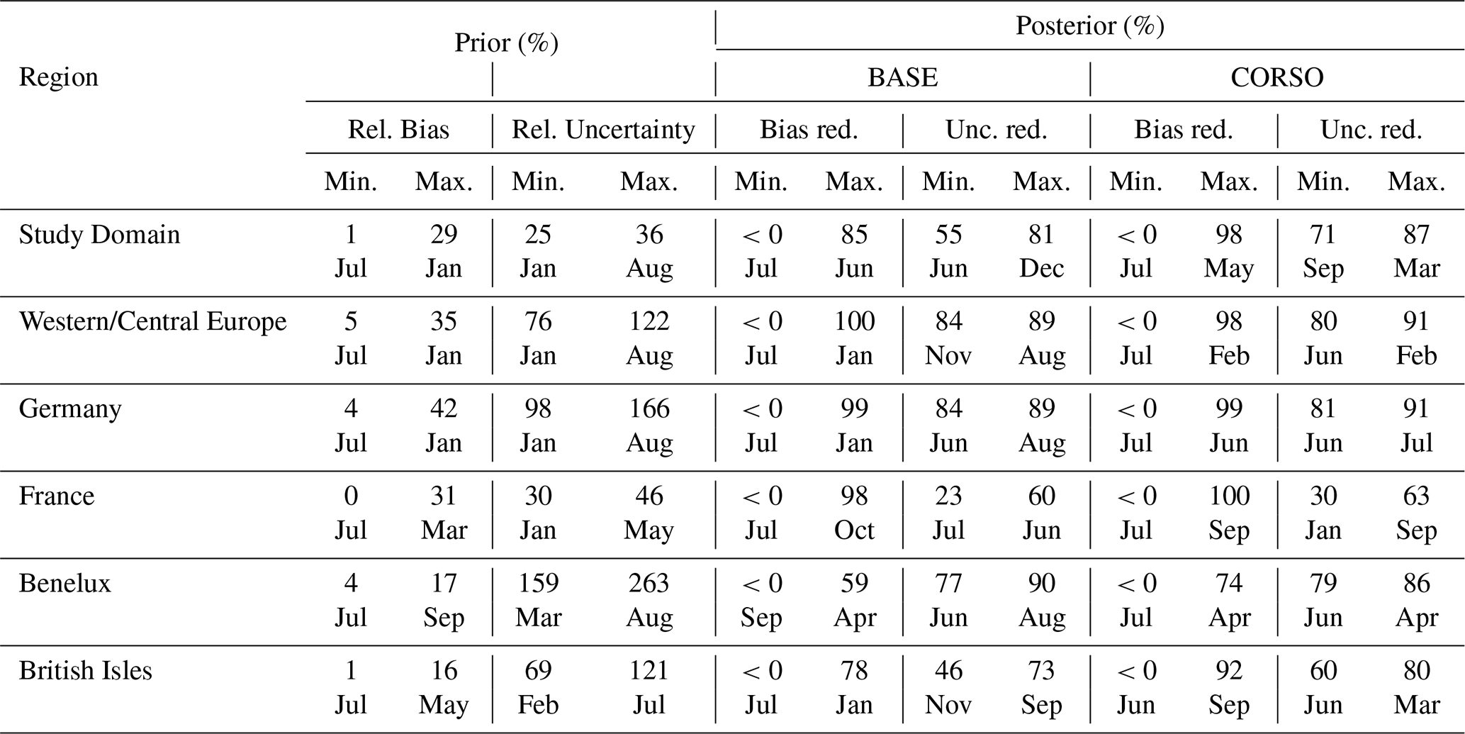
Table 3 Summary of prior relative bias and uncertainty, and posterior bias and uncertainty reductions for the BASE and CORSO experiments. All values are in percent. <0 values indicate cases where the posterior bias is greater than the prior bias. Bias and uncertainty reductions are calculated as described in Eq. (4).

4.2.2 Impact of selecting Δ¹⁴CO₂ flask samples using the ffCO₂ and ffCO thresholds

We compare the CORSO_ffCO2 and CORSO_ffCO2_ffCO experiments against the original CORSO setup to evaluate the impact of selecting Δ¹⁴CO₂ flask samples using fossil CO₂ and CO thresholds. This analysis focuses on Western/Central Europe (WCE) and Germany (Fig. 5), which showed the best performance in Sect. 4.2.1. Table 4 summarizes the minimum and maximum bias and uncertainty values, their respective posterior reductions, and the corresponding months.

In WCE, the CORSO experiment shows a bias reduction of between 81 % and 98 % during winter months, with uncertainty reductions between 82 % to 91 %. The CORSO_ffCO2 experiment performs similarly in winter, with bias reductions ranging from 71 % to 99 % and uncertainty reductions of 89 %–92 %. CORSO_ffCO2_ffCO also shows comparable performance during winter, with bias reductions of 79 %–97 % and uncertainty reductions of 81 %–94 %.

During the summer, differences between the experiments are more pronounced. In July, CORSO_ffCO2_ffCO shows the largest bias reduction (78 %), while CORSO and CORSO_ffCO2 show much weaker improvements (−42 % and 15 %, respectively). However, in June and August, CORSO and CORSO_ffCO2 perform better, with bias reductions between 70 % and 88 %, compared to 26 %–56 % for CORSO_ffCO2_ffCO. All three experiments show similarly strong uncertainty reductions throughout the year, with values consistently above 79 %.

In Germany, uncertainty reductions exceed 83 % across all months for all experiments. The largest differences in bias reduction occur during summer. CORSO_ffCO2 sperforms best between May and August, with reductions ranging from 48 % in July to 97 % in June. In contrast, CORSO shows a reduction as low as 4 % in August, and CORSO_ffCO2_ffCO reaches only 7 % in July. Overall, CORSO_ffCO2_ffCO tends to show the weakest summer bias reduction, with a maximum of 56 % in June.

In summary, while all three experiments lead to substantial improvements over the prior, selecting samples based solely on fossil CO₂, CORSO_ffCO2 provides the most consistent reductions in both bias and uncertainty, particularly during summer months, without requiring the additional CO threshold.

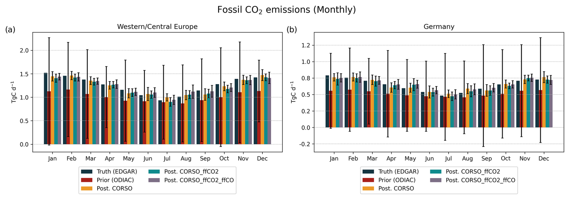
Figure 5 Monthly fossil CO₂ truth (black), prior (red), and posterior fluxes from the CORSO (yellow), CORSO_ffCO2 (teal), and CORSO_ffCO2_ffCO (purple) experiments for (a) Western/Central Europe and (b) Germany. Vertical error bars indicate the associated ±1σ uncertainties from a Monte Carlo ensemble of 25 members.

Table 4 Summary of the prior bias and uncertainty and the posterior bias and uncertainty reductions for the CORSO_ffCO2 and CORSO_ffCO2_ffCO experiments. All values are in percentage.

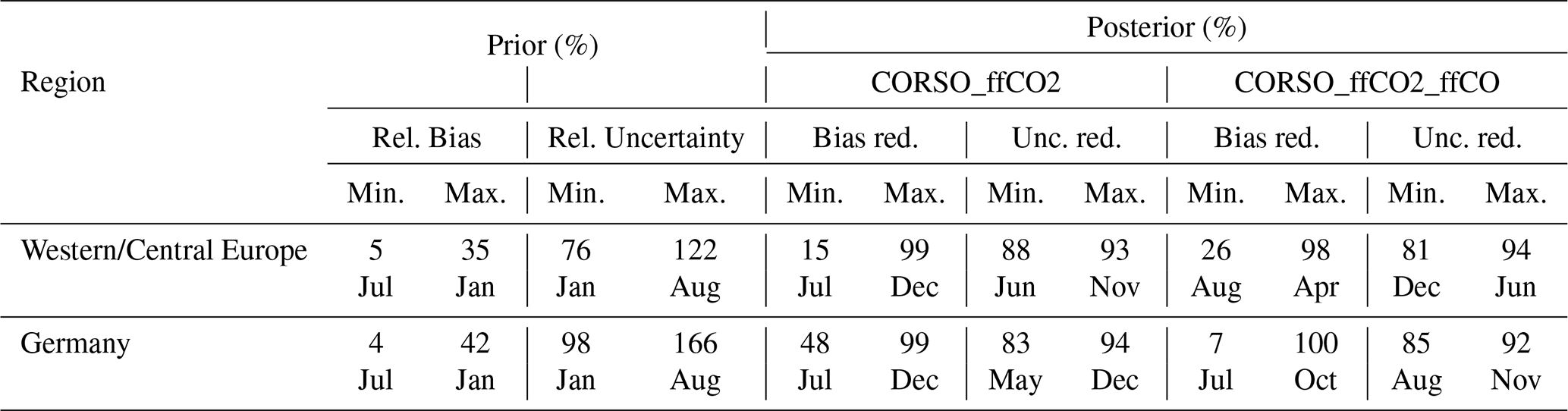
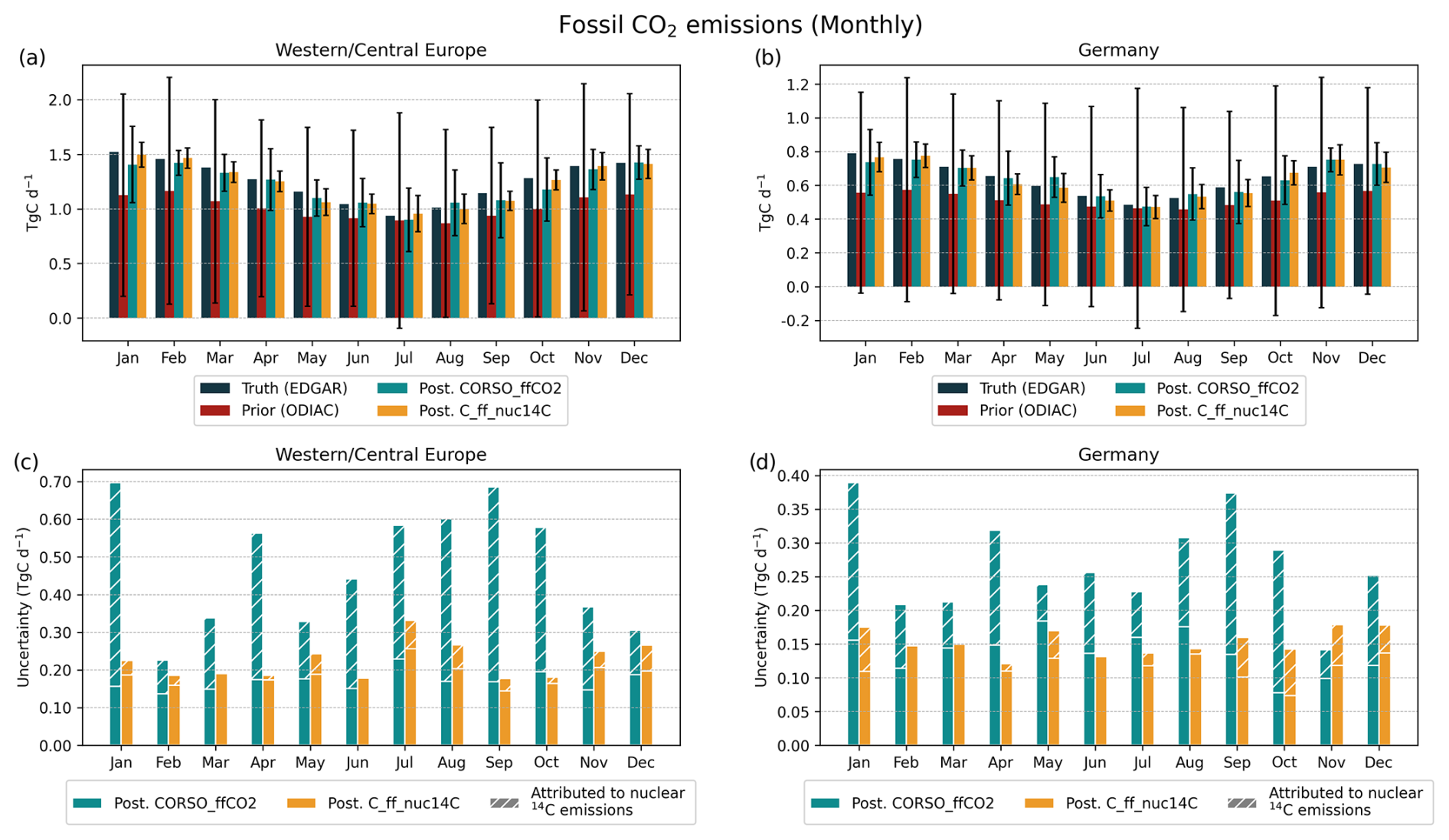
Figure 6 Monthly fossil CO₂ truth (black), prior (red), and posterior fluxes from the CORSO_ffCO2 (teal), and CORSO_ffCO2_nuc14C (yellow) experiments for (a) Western/Central Europe and (b) Germany. Panels (c) and (d) show the posterior uncertainty in fossil CO₂ flux estimates for the CORSO_ffCO2 (teal) and CORSO_ffCO2_nuc14C (yellow) experiments for Western/Central Europe and Germany, respectively. Hatched segments represent the portion of posterior uncertainty attributed to nuclear ¹⁴C emissions.

4.2.3 Impact of nuclear power facilities

Panels (a) and (b) of Fig. 6 show the monthly fossil CO₂ flux estimates for Western/Central Europe and Germany, respectively. The posterior estimates from CORSO_ffCO2 and CORSO_ffCO2_nuc14C are broadly consistent throughout the year and show good agreement with the truth (EDGAR). However, there are small differences in winter months, particularly in January and February, where CORSO_ffCO2_nuc14C slightly underestimates emissions compared to CORSO_ffCO2. This reflects the effect of excluding samples potentially influenced by nuclear ¹⁴C emissions. Despite these differences, both experiments reduce the prior bias and follow the seasonal cycle well in both regions.

Panels c and d of Fig. 6 show the corresponding posterior uncertainties. These are based on the Monte Carlo ensembles described in Sect. 3.6.4, and represent the contribution of nuclear ¹⁴C emissions to the posterior uncertainty. Without accounting for nuclear emissions, both experiments show similar uncertainty levels across the year. In Western/Central Europe, posterior uncertainties range from 0.1 to 0.3 Tg C d⁻¹ (12 %–29 %), and in Germany from 0.1 to 0.2 Tg C d⁻¹ (14 %–38 %).

However, when the impact of nuclear ¹⁴C emissions is included, the influence of the sampling selection strategy is more clearly reflected in the results. In Western/Central Europe, CORSO_ffCO2_nuc14C maintains posterior uncertainties within 16 %–37 %, similar to those without nuclear impact. In contrast, the CORSO_ffCO2 experiment shows a wider range of uncertainty (19 %–73 %), with the additional uncertainty attributable to nuclear emissions ranging from 8 % to 55 %. A similar pattern is observed in Germany: CORSO_ffCO2_nuc14C shows uncertainty values between 24 % and 35 %, while CORSO_ffCO2 reaches up to 77 %.

The spatial distribution of the annually aggregated posterior uncertainties attributed to nuclear emissions for the CORSO_ffCO2_nuc14C relative to CORSO_ffCO2 experiments is shown in Fig. 7. The largest uncertainties (Fig. 7b), are found in the UK, northern France, and the Benelux region, where the uncertainty often exceeds the posterior emissions (>100 %). This uncertainty can also extend to countries without nuclear facilities, such as Poland, where we observe uncertainties as high as 35 % per grid cell. Nevertheless, in the CORSO_ffCO2_nuc14C (Fig. 7a) we find areas in the UK and the Benelux region with uncertainties attributed to nuclear emissions as high as 49 %, which may indicate regions in which the sampling strategy, despite aiming to minimize nuclear contamination, still includes sites with substantial nuclear influence.

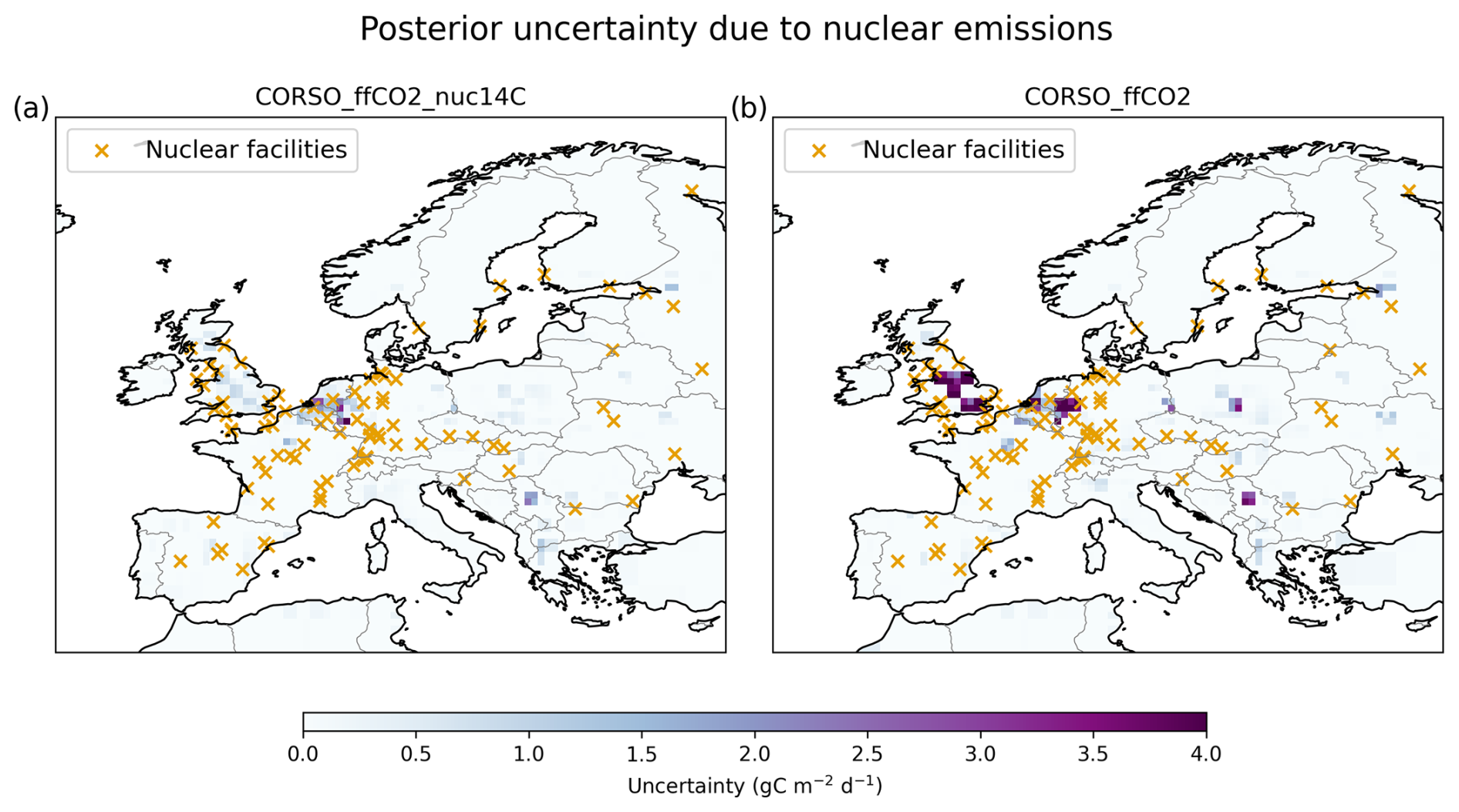
Figure 7 Spatial distribution of the annual posterior fossil CO₂ emission uncertainty due to nuclear emissions for the (a) CORSO_ffCO2_nuc14C and (b) CORSO_ffCO2 experiments. Yellow crosses show the location of nuclear facilities.

5 Discussion

In this study, we simulate the intensive Δ¹⁴CO₂ flask sampling campaign during the CORSO project under different scenarios to address the challenge of using atmospheric Δ¹⁴CO₂ measurements for the estimation of fossil CO₂ emissions in Europe, a continent with a high density of active nuclear facilities. Radiocarbon emissions from these facilities can significantly distort atmospheric Δ¹⁴CO₂ signals, particularly during periods with low biospheric activity, masking fossil signals and introducing attribution biases (Bozhinova et al., 2014; Maier et al., 2023). To mitigate this, we evaluate the benefit of taking more frequent, short-duration samples (1 h instead of 14 d) throughout the year, increasing the likelihood of capturing periods with strong fossil CO₂ signals and low nuclear interference.

While the OSSE simulations are based on 2018 conditions, future real-world flask samples may still be influenced by radiocarbon emissions from decommissioned facilities. For example, Philippsburg 2, a pressurized water reactor (PWR) located near Karlsruhe, was shut down in December 2019, yet reported ¹⁴CO₂ discharges rose from 33 Bq in 2018 to 7.8 GBq in 2021, according to the EU RADD database (https://europa.eu/radd/index.dox, last access: 17 June 2025). This increase is associated with a shift in chemical speciation during decommissioning: while PWRs mainly emit ¹⁴CH₄ during operation, emissions become dominated by ¹⁴CO₂ during dismantling and waste treatment activities (Kuderer et al., 2018). Thus, despite the official shutdown of all German NPPs in April 2023, residual emissions may continue to influence Δ¹⁴CO₂ observations at stations like KIT during the 2024 campaign. At the same time, while Germany has phased out nuclear energy, several other European countries are expanding their nuclear capacity. France, the UK, Finland, and others have recently built or approved new reactors. This growing heterogeneity in nuclear policy means that radiocarbon emissions will likely remain a persistent challenge for fossil fuel source attribution using Δ¹⁴CO₂, and must be accounted for in future sampling strategies and inversion frameworks.

We first study the impact of Δ¹⁴CO₂ flask samples on the estimation of fossil CO₂ emissions by comparing the BASE experiment (using only integrated samples) with the CORSO experiment (including additional flask samples). Our findings reveal that, in general, the CORSO experiment provides a better estimation of emissions, particularly in winter months, and significantly reduces both bias and uncertainty compared to the BASE experiment. In the study domain, the CORSO experiment has a larger bias reduction and uncertainty reduction throughout most months, except for June and July, where the BASE experiment performs better. June and July are the months with the lowest fossil emissions of the year, as already found by Levin et al. (2020) in real observations and in this study with synthetic observations. Levin et al. (2020) found that fossil CO₂ events are particularly rare during the summer months, with very few significant events occurring between May and August. In these months, fossil CO₂ mixing ratios rarely exceeded 4–5 ppm at various stations. Since integrated samples cover longer periods and hence larger areas than flask samples, they are more likely to capture the cumulative effects of low but steady emissions over time, providing a better estimate during months with fewer significant fossil CO₂ events. This extended sampling period compensates for the lower frequency of elevated emissions, ensuring that even minor contributions are accounted for, which may explain the improved performance of the BASE experiment during the summer months.

As already stated by Levin et al. (2020), it is necessary to perform a sample selection of Δ¹⁴CO₂ flask samples to ensure a good constraint on fossil CO₂ emissions, based on the thresholds defined for CO₂ and CO. This approach helps to guarantee the detection limit of the Δ¹⁴CO₂ analysis, isolate fossil CO₂ signals from other sources of CO₂ and make a more efficient use of flask samples. However, this method also carries the risk of predominantly monitoring the same dominant point sources, which may not represent a comprehensive mixture for the region. To mitigate this risk, it is essential to balance the selection criteria to capture a more representative mix of regional sources. Furthermore, the uncertainty of the Δ¹⁴CO₂ analysis requires a minimum signal strength to ensure the accuracy of the measurements. This requires the inclusion of samples that meet the fossil CO₂ content thresholds and provide a sufficient radiocarbon signal to reduce the analytical uncertainty. Ensuring a minimum signal strength is crucial for the reliability of the Δ¹⁴CO₂ data, as low signal samples can lead to higher relative errors and less confidence in fossil CO₂ estimates.

The analysis of the experiments shows that there is not a single experiment that consistently outperforms the others across all seasons and regions. Although each approach (CORSO, CORSO_ffCO2, and CORSO_ffCO2_ffCO) offers its own strengths in bias and uncertainty reduction, particularly during the winter months, none stands out as consistently better across all scenarios. Implementing the selection strategy for the CORSO_ffCO2 experiments in a real-world operational setting would require performing near-real-time simulations to estimate the ffCO₂ component. The CO threshold was introduced because this can be obtained from continuous CO measurements, and can be calculated as the CO enhancement with respect to the background instead of ffCO (Levin et al., 2020). From the perspective of OSSEs, the results suggest that the selection of samples may not be as critical as ensuring good coverage of sampling events throughout the year. The findings suggest that maintaining a well-distributed and frequent sampling schedule provides a more representative and effective basis for accurately estimating fossil CO₂ emissions than relying heavily on strict sample selection criteria. However, when accounting for nuclear ¹⁴CO₂ contamination, careful sample selection becomes essential to minimize biases and uncertainties.

In Europe, with more than 170 operational reactors and two reprocessing plants, nuclear contamination significantly impacts Δ¹⁴CO₂ samples. Maier et al. (2023) highlight that the median nuclear contamination at ICOS sites accounts for about 30 % in day-and-night integrated samples and 15 % in midday integrated samples, leading to substantial underestimation of fossil CO₂ estimates if not corrected. Similarly, Graven and Gruber (2011) discuss the continental-scale enrichment of atmospheric Δ¹⁴CO₂ due to emissions from the nuclear power industry, which creates significant gradients that extend more than 700 km from nuclear sites in Europe. Their study demonstrates that the spatial scale of these gradients is sufficient to influence regional Δ¹⁴CO₂ levels, requiring high-resolution data from each nuclear reactor to accurately estimate Δ¹⁴CO₂ enrichment and mitigate biases in fossil CO₂ estimates (Graven and Gruber, 2011).

To assess the impact of nuclear contamination on fossil CO₂ estimates, we compared two sample selection experiments: one favoring low nuclear influence (CORSO_ffCO2_nuc14C) and one selecting samples with potentially high nuclear influence (CORSO_ffCO2). While both experiments yielded emission time series that generally tracked the true emissions well, the experiment minimizing nuclear influence consistently resulted in lower posterior uncertainties, particularly across regions with high prior uncertainty, such as Benelux, eastern France, and western Germany. This highlights the added value of targeting samples that minimize contamination from radiocarbon sources unrelated to fossil emissions. Moreover, our results show that this nuclear-related uncertainty can propagate beyond the immediate vicinity of power plants, affecting regions without nuclear facilities, such as Poland. This finding supports earlier work by Graven and Gruber (2011), who documented the regional-scale influence of European nuclear facilities on atmospheric radiocarbon measurements. These findings highlight the need to adapt sampling strategies to the spatial distribution of nuclear activity. Although integrated samples are useful for capturing long-term trends, their reliability may be compromised in regions affected by nuclear emissions. In such cases, combining integrated and flask sampling, or selectively using integrated samples, can provide a more robust approach for estimating fossil CO₂ estimation.

In our perfect transport OSSEs implementation, we do not account for uncertainties due to transport model representation errors. Munassar et al. (2023) found that the use of different transport models, which help us to understand the model representation error, can result in differences of 0.51 Pg C yr⁻¹ (61 %) in the posterior NEE flux estimates over Europe. Their study uses continuous CO₂ observations selected at times when there is a better model representation. We note that these discrepancies, and more generally the model representation of integrated samples, may differ depending on the integration period. While short-term observations can be more sensitive to transport or mixing errors, longer integration periods (e.g. two weeks) may average out some of this variability, potentially reducing but also redistributing the associated model–data mismatches. This integration captures a mix of local and regional influences and is especially affected by diurnal circulation patterns. For example, high-altitude stations may sample polluted valley air transported upslope during the day and cleaner free tropospheric air descending at night due to mountain–valley winds. Moreover, model accuracy tends to be higher during well-mixed conditions (e.g., such as in the afternoon planetary boundary layer or in the free troposphere) compared to periods with stable stratification, such as during the nocturnal boundary layer or transition phases, which are more difficult to represent. Maier et al. (2022) study the performance of two modeling approaches using a Lagrangian model (STILT) in representing afternoon and nighttime 2-week integrated ¹⁴C-based ffCO₂ observations from Heidelberg: the surface source influence (SSI) approach, similar to our implementation with FLEXPART in which all emissions are assumed to occur at ground level, and the the volume source influence (VSI) approach in which there is a representation of the emission height and the plume rise of point source emissions, such as the emissions from power plants. Combining the SSI and VSI approaches, or developing hybrid frameworks that account for temporal and vertical variability in source influence, may be critical to improving the representation of integrated samples in inverse modeling applications using real data.

In some regions, the assigned prior uncertainty exceeds 100 % of the prior or true emissions (Fig. 4). This results from using relatively short spatial correlation lengths to allow the inversion to resolve emissions at finer scales, which in turn requires higher standard deviations to maintain consistent covariance structures. In practice, errors in fossil emission inventories likely exhibit broader spatial correlations, suggesting that a regionally or nationally defined uncertainty structure could be more appropriate. While our current approach may overestimate grid-scale uncertainties, it remains a reasonable approximation for testing the impact of observation strategies. Importantly, all experiments show consistent uncertainty reductions, even though posterior uncertainties were larger than the prior bias in some regions during summer months. While this limits the resolution at which emissions can currently be reported with confidence, the consistent uncertainty reductions across all experiments highlight the potential for further improvement. Refining the prior uncertainty structure and applying the sampling strategies proposed in this study can support more accurate fossil CO₂ estimates at finer spatial and temporal scales.

In some regions, the assigned prior uncertainty exceeds 100 % of the prior or true emissions (Fig. 4). This results from the way the uncertainties are set up in LUMIA: the grid-cell scale uncertainties (σ_x) are scaled to match a target annual, category-specific total uncertainty over the whole domain. Therefore, the longer the spatial and temporal correlation lengths, the lower the standard deviations must be to achieve the same total variance. For fossil fuel emissions, the total uncertainty for Europe was based on the annual difference between the prior and the synthetic truth, derived from two independent, state-of-the-art emission inventories. The spatial correlation length was set to 200 km, under the assumption that the observation network is dense enough to resolve emission patterns at that scale. Both settings are reasonable when considered separately, but their combination leads to unrealistically large prior uncertainties at the grid-cell and even regional scale. This could be addressed by using much longer error correlation lengths, better reflecting the true ones. However, doing so would limit the use of the observation network’s full potential in regions where it can resolve finer-scale patterns. Developing and testing an approach to set prior uncertainties that better balances realism in error correlations with the resolution capacity of the observation network should be a priority for future LUMIA developments. Even if the current approach is not fully optimal and limits the interpretability of some uncertainty estimates, it still provides a valid framework for evaluating the impact of the different ¹⁴C-based sampling strategies. It should not affect the relative performance of the inversions, especially in terms of error reduction. LUMIA inversions are, in general, more sensitive to the correlation structure than to the absolute uncertainty levels, particularly in regions with good observational coverage (Monteil and Scholze, 2021).

6 Conclusions

In this study, we find that adding regular Δ¹⁴CO₂ flask sampling to the integrated sampling (CORSO) generally provides better emission estimates than using only integrated samples (BASE), particularly during the winter months. However, the BASE experiment performed better than CORSO during low-emission months such as June and July. We also find that the selection of synthetic Δ¹⁴CO₂ flask samples according to their fossil contribution did not show significant improvements compared to the simpler CORSO approach. However, when samples were selected according to their level of nuclear contamination, the experiments showed that selecting samples with low nuclear contamination led to a substantial reduction in uncertainty, particularly in regions like Western/Central Europe and Germany. In contrast, selecting samples with potentially high nuclear contamination resulted in higher uncertainties, especially during the summer months.

Therefore, we recommend prioritizing the selection of Δ¹⁴CO₂ flask samples based on their potential nuclear contamination, given the limited knowledge about the temporal emission profiles of most nuclear facilities in our model domain. It is also necessary to perform a site-specific revision of the CO, ffCO₂, and nuc¹⁴C thresholds to adjust these values to the intensity of the fluxes measured at each station. This is also important for the Δ¹⁴CO₂ integrated samples. Although they can help to better estimate fossil CO₂ in periods of low emissions such as summer, long integration times can also result in large radiocarbon nuclear emissions being captured, increasing the posterior uncertainty of the estimates. In real inversions, these integrated samples can also have large representation errors. A promising approach to account for these representation error in an inversion is the implementation of the volume source influence (VSI) approach as proposed by Maier et al. (2022).

Despite the advancements shown by these experiments, high posterior uncertainties during the summer months remain a challenge. This limits the reliability of monthly emission estimates, underscoring the need for further refinement in both selection strategies and inverse modeling techniques. Until these challenges are adequately addressed, the utility of monthly emissions estimates will remain limited, pointing to the importance of performing an appropriate uncertainty characterization of fossil emissions.

Appendix A: Additional site-level time series for Δ¹⁴CO₂ synthetic and observed samples

A1 Thresholds

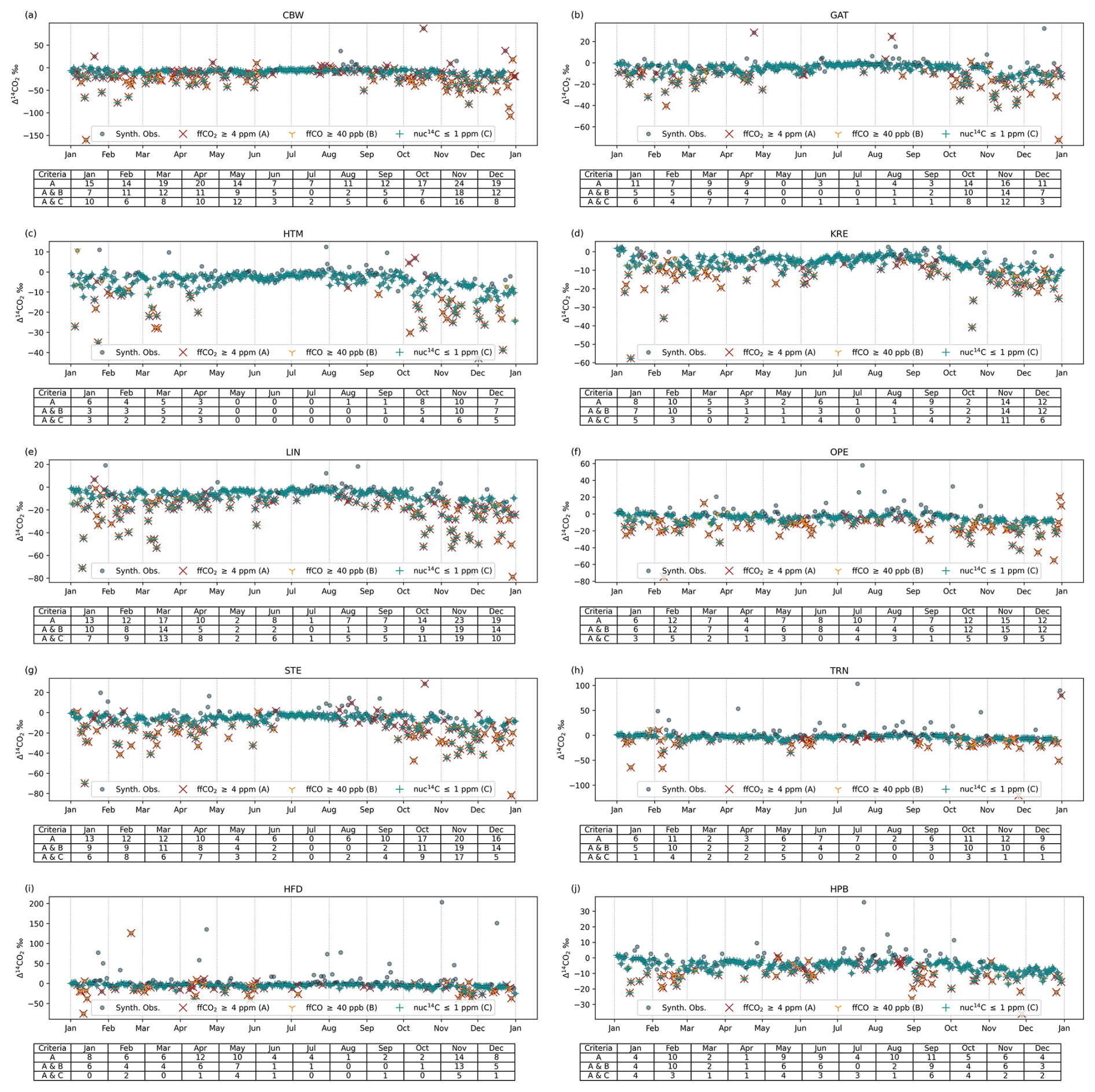
Figure A1 Synthetic Δ¹⁴CO₂ flask samples at the 10 remaining sampling sites selected for the intensive sampling campaign during the CORSO project. The tables below each figure show the number of synthetic observations per month that meet the ffCO₂ threshold (red cross), the ffCO₂ and ffCO (yellow tri) thresholds, and the ffCO₂ and nuc¹⁴C (green cross) thresholds.

A2 Comparison between real and modeled observations

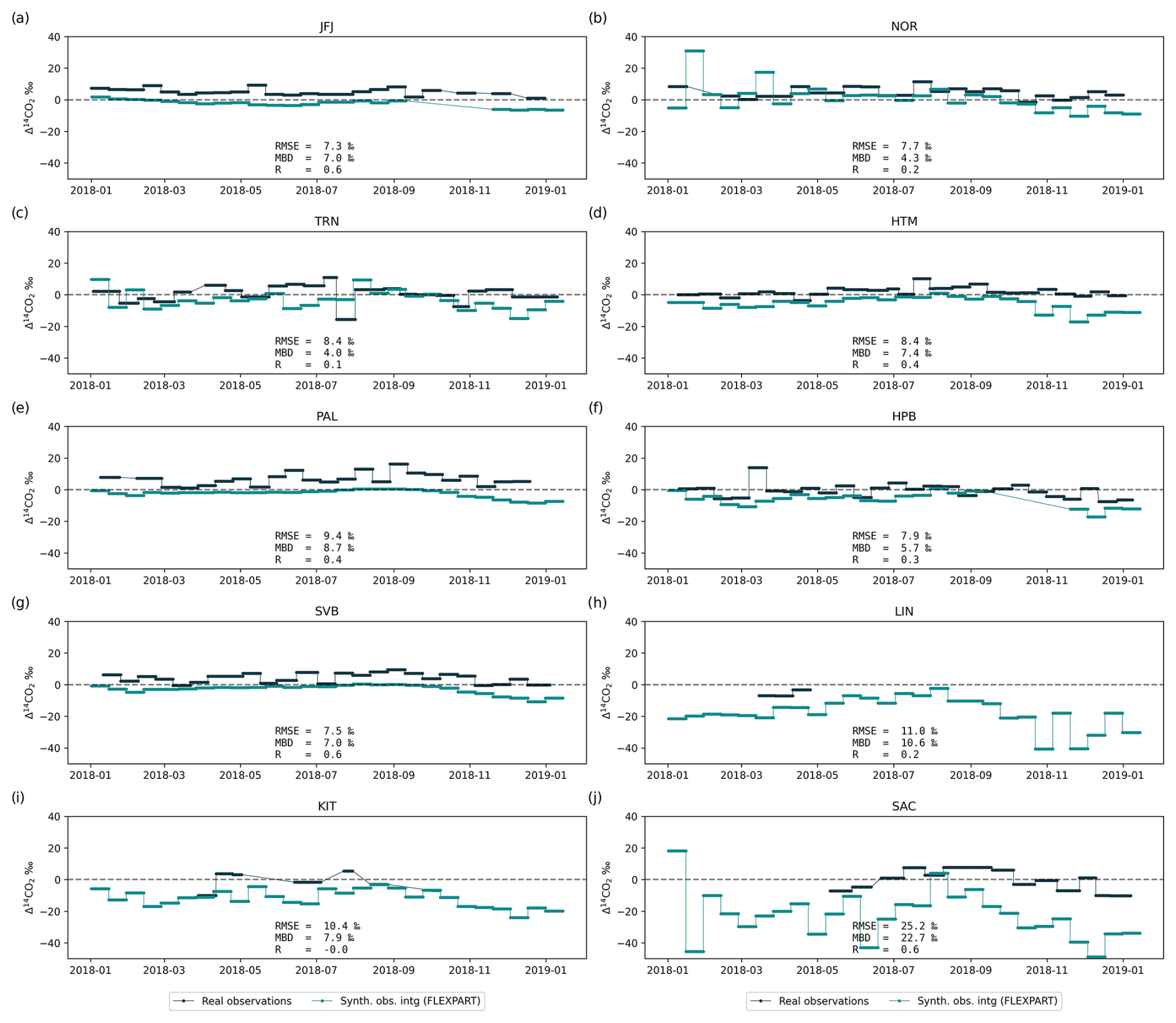
Figure A2 Comparison of the available real Δ¹⁴CO₂ integrated samples (black) (ICOS RI et al., 2024) with the modeled background observations (red) and synthetic observations (teal) at ten ICOS sites.