Relation between total vertical column density and near-surface NO₂ based on in situ and Pandora ground-based remote sensing observations

Nitrogen dioxide (NO₂) is a major pollutant that at high concentrations may affect human health. It is also a photochemically reactive gas that is important for the oxidation potential of the atmosphere and acts as a precursor for the formation of aerosol particles and ozone. However, monitoring of near-surface (NS) NO₂ faces the challenge of spatial discontinuity due to large distances between ground-based monitoring stations, whereas satellite remote sensing provides total vertical column density (VCD) that is related to near-surface (NS) concentrations in a complicated manner. In this study, the relation between total VCD and NS concentrations of NO₂ was analyzed based on total VCD from remote sensing observations using a ground-based Pandora spectrometer and NS NO₂ concentrations from in situ observations. Both instruments were located at the Beijing-RADI site (Beijing, China) during January 2022. The ratio between total VCD and NS NO₂ concentrations varies throughout the day with substantially different relations in the morning and afternoon. During the night and morning, the atmosphere was vertically stratified, with disconnected layers that prevented vertical mixing of atmospheric constituents. In the afternoon, these layers connected, allowing for vertical mixing and transport between the surface and the top of the boundary layer. Thus, the prohibition of vertical transport in the morning and the mixing in the afternoon resulted in different relations between the total VCD and NS NO₂ concentrations. These different relationships have consequences for the use of satellite remote sensing to estimate NS NO₂ concentrations.

1 Introduction

Nitrogen dioxide (NO₂) can have adverse effects on human health (Eum et al., 2022, 2019; Nordeide Kuiper et al., 2021; Kornartit et al., 2010). NO₂ plays an important role in atmospheric chemistry and acts as a precursor for the formation of ozone and secondary aerosols in the atmosphere. The major sources of NO₂ are fossil fuel burning, such as power plants, traffic, and households. Because of these anthropogenic sources, together with the relatively short atmospheric lifetime of NO₂, high tropospheric NO₂ concentrations are usually observed near highly industrialized regions (van der A et al., 2006), densely populated agglomerations (de Souza et al., 2022), and power plants (Tang et al., 2024), as well as along major highways (Goldberg et al., 2021) and shipping lanes (Ding et al., 2018). In addition, NO₂ is produced from some natural sources such as lightning and soil emissions.

Concentrations of NO₂ in the atmosphere can be measured using satellite-based sensors providing total and tropospheric column densities, ground-based remote sensing using MAX-DOAS or Pandora instruments, or in situ instruments. Satellite remote sensing is currently a widely used technique, for example, using the Ozone Monitoring Instrument (OMI, Levelt et al., 2006) on the Aura satellite and the TROPOspheric Monitoring Instrument (TROPOMI, Veefkind et al., 2012) on the Sentinel-5 Precursor (S5P) satellite. Satellite data show that the total vertical column density (VCD) of NO₂ is highly variable in space and time (e.g., Lamsal et al., 2014; Fan et al., 2021). Duncan et al. (2016) analyzed global NO₂ observed by OMI from 2005 to 2014 and found that NO₂ levels were initially high over China but had significantly decreased over the Beijing, Shanghai, and the Pearl River Delta (PRD) regions in 2014, in response to pollution control measures. In particular, over the PRD region, the NO₂ concentrations decreased by about 40 %. Also, in the following years, the NO₂ concentrations over China have substantially diminished in response to the implementation of emission reduction policy (e.g., van der A et al., 2017; Fan et al., 2021; de Leeuw et al., 2021) and fell below the 2008 level in 2017 (Zhao et al., 2023). However, the decrease seems to have flattened in recent years (Fan et al., 2021).

The Pandonia Global Network (PGN) of Pandora Spectrometer Instruments was established in 2018 (http://www.pandonia-global-network.org/, last access: 10 July 2024) to provide “quality observations of total column and vertically resolved concentrations of a range of trace gases”. The PGN data are used, for instance, for the validation of products from environmental satellites. However, the comparison of OMI total VCD of NO₂ with Pandora observations at six sites in South Korea and the USA by Herman et al. (2019) showed that the mean and daily Pandora NO₂ concentrations were 50 % or more higher than those retrieved from OMI at sites that were frequently contaminated, such as Seoul, Busan, and Washington, DC. Tzortziou et al. (2018) reported that Pandora total VCD of NO₂ during the KORUS-AQ coastal cruise experiment (Tzortziou, et al., 2015) was 10 %–50 % higher than OMI-derived total VCD of NO₂. The relationship between total VCD and near-surface (NS) concentrations of NO₂ was complex according to the analysis of data from the DISCOVER-AQ campaign in the Baltimore–Washington region in July 2011; the discrepancies were suggested to be caused by the large field of view of OMI (Flynn et al., 2014; Knepp et al., 2015; Reed et al., 2015; Tzortziou et al., 2015). Preliminary validation of total VCD of NO₂ from the Ozone Mapping and Profiler Suite (OMPS) aboard the joint NASA/NOAA Suomi National Polar-orbiting Partnership (Suomi NPP) satellite by Huang et al. (2022) in the USA showed that OMPS total VCD of NO₂ tends to be lower in polluted urban areas and higher in clean areas/events than Pandora observations. Ialongo et al. (2020) and Zhao et al. (2020) obtained similar results from the validation of TROPOMI total VCD of NO₂ using PGN data, but the differences were significantly smaller than those for the OMI and OMPS data with a coarser spatial resolution than TROPOMI. The validation of TROPOMI total VCD versus Pandora data at the Beijing-RADI site shows the good performance of TROPOMI (Liu et al., 2024). It is noted that Liu et al. (2024) resampled the TROPOMI data to a spatial resolution of 100 × 100 m², i.e., similar to that of the Pandora observation area.

Satellite-derived total VCD of NO₂ data are often used to determine trends (e.g., van der A et al., 2017; Fan et al., 2021) but, in view of the above, the relation between total VCD and NS concentrations of NO₂ is more complex. For instance, Fan et al. (2021) discussed the total VCD/NS relationship for selected major urban regions in China during the first 20 weeks after the COVID-19 lockdown and observed substantial differences (their Fig. 9). Chang et al. (2022) analyzed data from the Geostationary Environment Monitoring Spectrometer (GEMS) Map of Air Pollution (GMAP) campaign conducted during 2020–2021. Their results indicate that total VCD and NS concentrations of NO₂ exhibit a stronger correlation under advective boundary layer conditions at high wind speeds, where the vertical distribution of NO₂ is more uniform. In contrast, the presence of plumes from large point sources, either decoupled from the surface or transported from nearby cities, enhances the vertical heterogeneity of NO₂. These plumes contribute to a less consistent relationship between total VCD and NS concentrations of NO₂. Similarly, Liu et al. (2024) showed different relations between total VCD and NS concentrations of NO₂ for low and high concentrations, which are qualitatively explained in terms of transport and local emissions. Moreover, Thompson et al. (2019), using data from the KORUS-AQ coastal cruise experiment, reported that there is no consistent correlation between total VCD and NS concentrations of NO₂ across different cases and that the relation between total VCD and NS concentrations of NO₂ is complex. Thus, to accurately assess NO₂ pollution in China and its effects on air quality, accurate ground-based observations are needed.

Although a large number of ground-based NO₂ observation stations have been established in China since 2012 by the China National Environmental Monitoring Center (CNEMC) of the Ministry of Ecology and Environment of China (MEE) for the provision of the ground-based monitoring data (available at http://www.mee.gov.cn/, last access: 8 July 2024), there are still large areas for which no data are available. Satellite data can fill these gaps by converting satellite observations of aerosols and trace gases from total VCD and NS concentrations. Such data are usually provided by sensors flying on polar-orbiting satellites with global coverage but with a single overpass per day, which at most latitudes cannot provide the daily variability of NO₂ characteristics. However, with the launch of geostationary satellites, spatial and temporal distributions of NO₂ concentrations can be obtained within the satellite field of view throughout the day. The GEO-KOMPSAT-2B geostationary satellite, launched by the National Institute of Environmental Research (NIER) under the Ministry of Environment, South Korea, in February 2020, carries the Geostationary Environment Monitoring Spectrometer (GEMS), which provides high-resolution measurements of total VCD of key air quality components (Kim et al., 2020). With the launch of GEMS, the Asian region was the first to achieve coordinated hour-by-hour monitoring of pollutants. GEMS will form a constellation of satellites to monitor air quality globally with high temporal and spatial resolution, together with the Tropospheric Emissions: Monitoring Pollution (TEMPO) mission, launched by NASA on 7 April 2023 to cover the North American region (https://tempo.si.edu/overview.html, last access: 18 April 2025) and Sentinel-4, planned to be launched on the Meteosat Third Generation Sounder (MTG-S) by the European Organisation for the Exploitation of Meteorological Satellites (EUMETSAT) in 2025 (https://www.eumetsat.int/meteosat-third-generation-sounder-1-and-copernicus-sentinel-4, last access: 18 April 2025).

While geostationary satellites enable continuous daytime observations of total VCD of NO₂, discrepancies between total VCD and NS concentrations of NO₂ remain a critical challenge. The weak correlation between NS NO₂ concentrations and satellite-derived total VCD of NO₂ (Lamsal et al., 2014) is closely tied to differences in their vertical distribution, atmospheric lifetimes, and chemical reaction pathways (Xing et al., 2017). Despite extensive efforts to derive NS NO₂ concentrations from total VCD measurements (Chang et al., 2025; Wei et al., 2022; Zhang et al., 2022; Dou et al., 2021), the dynamic complexity of the planetary boundary layer introduces substantial uncertainties. Moreover, prior studies have emphasized the roles of vertical NO₂ distribution (Sun et al., 2023; Zhang et al., 2023; Kang et al., 2021) and regional pollutant transport contributions (Yin et al., 2025; Dong et al., 2020; Chang et al., 2019; Li et al., 2017), but research explicitly linking regional transport processes to vertical NO₂ concentration gradients and elucidating their interactive effects remains limited. Song et al. (2024) obtained NS NO₂ concentrations based on the Himawari-8 geostationary satellite using machine learning, which showed good performance in the noon and afternoon and relatively poor performance in the morning. These knowledge gaps are further exacerbated by satellite data limitations in resolving NS pollution, which has direct implications for human health assessments. To address these challenges, we need to integrate ground-based remote sensing observations with in situ NS NO₂ measurements to investigate vertical decoupling phenomena and the influence of distinct pollutant transport pathways on NS NO₂ pollution dynamics.

The first operational Pandora instrument in China was installed at the Beijing-RADI site in 2021, for the ground-based remote sensing of several trace gases, including NO₂. The Beijing-RADI Pandora instrument is part of the PGN network, and all data are publicly available via the PGN website (https://data.pandonia-global-network.org/Beijing-RADI/Pandora171s1/, last access: 22 January 2025) within 1 d of the observations. The aim of this study is to analyze the relationship between total VCD of NO₂ obtained by remote sensing and NS measurements during a field experiment at the Beijing-RADI site during 10–29 January 2022. In order to better determine and understand the relation between total VCD and NS concentrations of NO₂, we also used auxiliary data such as simultaneous measurements of PM_2.5 mass concentrations, lidar observations, meteorological parameters, and satellite observations. Section 2 presents the experiments and data, Sect. 3 presents the main results, and the conclusions and discussion are presented in Sect. 4.

2 Materials and method

2.1 Site description

Beijing is a metropolis with an area of 16 800 km² and a population of nearly 22 million (2023) (https://worldpopulationreview.com/world-cities/beijing-population, last access: 22 January 2025). High mountains are located to the north and west of Beijing (Fig. 1). The rapid economic development of Beijing and the topography of the area lead to the emission of pollutants that may either disperse or accumulate, depending on wind direction and wind speed. During northwesterly winds, clean air is transported from the mountains, whereas during southerly winds, polluted air is transported from the highly industrialized North China Plain. The southerly airflow is blocked by the mountains to the west and north, and thus pollution accumulates, in particular, during certain weather conditions conducive to the formation of smog, such as low wind speed. Photochemical processes may further contribute to the build-up of pollution that may result in the formation of haze.

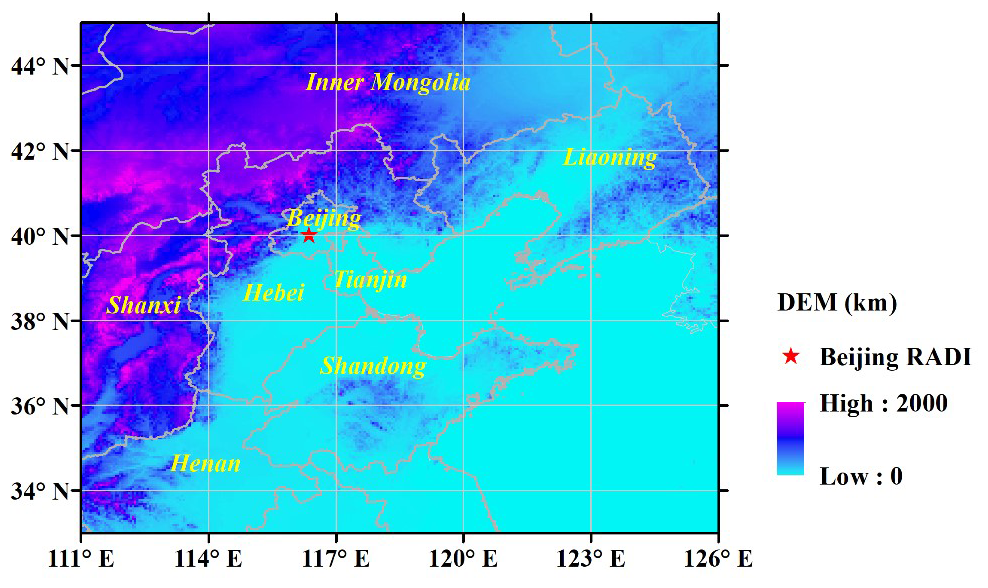
Figure 1 Digital elevation map of the study area showing the location of the Beijing-RADI site (40.004° N, 116.379° E, altitude at 59 m) (red star) and surrounding mountains.

The Beijing-RADI site is located on the roof (22 m above the surface) of the Aerospace Information Research Institute of the Chinese Academy of Sciences (40.004° N, 116.379° E, elevation 59 m), which in turn is located in the north of Beijing between the Fourth and Fifth Ring Roads at the edge of the Olympic Park. The site is representative of an urban background affected by vehicle exhaust, combustion, and domestic emissions, including those from heating during wintertime.

A short-term field experiment was carried out at the Beijing-RADI long-term observation site during 10–29 January 2022. Pandora provided total VCD of NO₂ concentrations in four layers; information on the spatial distribution of total VCD of NO₂ was obtained from TROPOMI; and a lidar provided aerosol backscatter profiles, showing the vertical structure and evolution of the atmospheric boundary layer. The NS parameters were measured with instrumentation mounted near the Pandora on the roof of the AirCAS building, as described in the following sections.

2.2 Observations of column-integrated parameters and vertical profiles

2.2.1 Pandora

Pandora is a UV-visible spectrometer that can provide high-quality measurements of spectrally resolved direct-sun/lunar or sky scan radiances. It uses direct solar measurements to obtain total VCD of NO₂ and sky measurements to obtain the vertical layer concentrations of NO₂, with a field of view of 2.6° in direct-sun mode and 1.5° in sky mode (Cede, 2024). Based on the Beer–Bouguer–Lambert law, the spectra observed at 400–470 nm in direct-sun mode are used to invert total VCD of NO₂ using the differential optical absorption spectroscopy (DOAS) technique of trace gas spectral fitting. Pandora's direct-sun measurements depend only on the geographic location with a known solar zenith angle, which simplifies the air mass factor for correction of the atmospheric light path (Chang et al., 2022). Pandora measures total VCD of NO₂ with a clear-sky precision of 0.01 DU and a nominal accuracy of 0.1 DU (Herman et al., 2009). In view of this high precision, we use total VCD of NO₂ from the nvs3 product in this study and select data with a quality control flag of L10. Diffuse (scattered) radiation is measured at five pointing zenith angles (PZAs) in sky mode that, together with the direct sun measurement, provides information on the tropospheric VCD and on the surface concentrations. The PZAs are 0, 60, 75, 88°, and the maximum angle taken was 89°. The measurements are taken in a V shape (all angles are measured twice around a central angle), as described in Cede (2024). Four partial columns of NO₂ concentrations are provided by the Pandora inversion. The first step is the estimation of the effective height corresponding to a given PZA and then the calculation of differential air mass factors for the NO₂ and the air gas for each layer. The profile shape of the partial columns is determined as a variation of the air-gas shape. The average number density of the NO₂ in each layer is then calculated. The partial column amounts can be obtained from the concentrations multiplied by the layer width as described in the Manual for Blick Software Suite (Cede, 2024), Sect. 6.7. The NO₂ of the partial column can be obtained from the uvh3 product, which was downloaded from the PGN website (https://pandonia-global-network.org, last access: 22 January 2025). We converted these partial column concentrations into layer-averaged volume mixing ratios and interpolated them to six standard levels (0.2, 0.5, 1.0, 1.5, 2.0, and 2.5 km) for visualization.

2.2.2 Lidar

A small lidar developed by the Hefei Institute of Physical Sciences, Chinese Academy of Sciences, was used for continuous measurements of aerosol backscatter profiles during day and night. The GBQ L-01 aerosol lidar consists of a laser, optical unit, control unit board, high-speed signal acquisition card, industrial motherboard, and communication module. The GBQ L-01 aerosol lidar uses a high-frequency pulse laser emitting linearly polarized light at a wavelength of 1064 nm. The optical unit consists of a transmitter and a receiver. The optical transmitter unit emits laser light pulses, which are expanded before they are emitted into the atmosphere. The optical receiver unit consists of a telescope that focuses the backscattered light onto an optical detector, which in turn is connected to an amplifier unit. The vertical and parallel polarized components of the backscattered light are separated by the polarizing prism in the receiving channel. The industrial motherboard carries lidar acquisition and control software and data analysis software to control the overall operation of the system.

2.2.3 TROPOMI

The TROPOMI (TROPOspheric Monitoring Instrument) is a passive-sensing hyperspectral nadir-viewing imager aboard the Sentinel-5 Precursor (S5P) satellite, launched on 13 October 2017. S5P flies at an altitude of 817 km in a near-polar sun-synchronous orbit. The local Equator overpass time in the ascending node is 13:30, and the repetition period is 17 d (KNMI, 2017). TROPOMI's four separate spectrometers cover wavelengths in the ultraviolet (UV), UV–visible (UV–VIS), near-infrared (NIR), and short-wavelength infrared (SWIR) spectral bands (Veefkind et al., 2012). The NO₂ used in this study is derived from spectral measurements of solar radiation in TROPOMI's UV–VIS wavelength bands (van Geffen et al., 2015, 2019). Compared to the relatively small field of view of the Pandora instrument, the size of the TROPOMI ground pixel (3.5 km × 5.5 × km; across × along track) is relatively large. In addition, only tropospheric vertical column densities (VCDs) for NO₂ were available during the time period of this study. The TROPOMI tropospheric VCDs for NO₂ are only used as a qualitative reference for upwind concentrations in the evaluation of effects of long-range transport using air mass backward trajectories and not for quantitative analysis. Furthermore, tropospheric NO₂ column densities are used because these are more representative of near-surface NO₂.

2.3 Near-surface measurement

2.3.1 Trace gas analyzer

The Thermo Fisher Scientific Model 42i Trace Level Chemiluminescence NO-NO₂-NO_x Analyzer (https://cires1.colorado.edu/jimenez-group/Manuals/Manual_NOx_42i.pdf, last access: 22 January 2025) was used to measure NS NO₂ concentrations. This instrument first transforms NO₂ into nitric oxide (NO) using a molybdenum NO₂ to NO converter heated to about 325 °C. Then, NO and ozone (O₃) react to produce a characteristic luminescence with an intensity linearly proportional to the NO concentration (Thermo Fisher Scientific, 2007). NO₂ values are derived by subtracting NO from NO_x measurements. Measurements were made every minute during the observation period.

2.3.2 Beta attenuation monitor

Ground-based near-surface PM_2.5 concentrations were measured using the beta attenuation monitor Met One BAM-102 equipped with a PM_2.5 inlet. The Met One BAM-1020 collects aerosol particles on glass filter tape. PM_2.5 is measured using beta rays generated by a small ¹⁴C source (https://metone.com/products/bam-1020/, last access: 18 April 2025). At the start of every measurement cycle, the flux of beta rays is measured across clean filter tape to determine a zero reading. Next, the filter tape is advanced and ambient air is sampled at the same spot, with a controlled airflow, thereby impregnating the tape with PM_2.5. After the sampling is completed, the tape retracts and PM_2.5 samples are dried (in an environment with relative humidity lower than 40 %, which removes most of the water content) by a built-in heater. Then the concentration of PM_2.5 collected on the filter tape is measured as described above. Samples are taken every hour.

2.3.3 Auxiliary meteorological data

In addition to the above observations, we also use weather maps, meteorological surface observations, and sounding observations published by the World Meteorological Organization (WMO) to aid in our analyses. Weather maps for the Asian region are published by the Korea Meteorological Administration and can be downloaded at http://222.195.136.24/chart/kma/data_keep (last access: 22 January 2025). We downloaded the surface and sounding observations of the meteorological station 54511 in Beijing, located at 39.93° N, 116.28° E, which is part of the WMO network. These data are available from the website of the University of Wyoming (http://weather.uwyo.edu/surface/, last access: 22 January 2025). Although this station is far away from our experimental site (about 23 km), it is representative of the macroscopic changes of the meteorological conditions in Beijing.

2.4 HYSPLIT model

To better understand the regional transport pathways and source regions at different altitudes, backward trajectories from the Hybrid Single Particle Lagrangian Integrated Trajectory (HYSPLIT; Draxler and Hess, 1998) model were used. The HYSPLIT model assumes that the parcel trajectory is formed through time integration and spatial differences while moving in the wind field. The path of the air mass is mainly related to the airflow situation, pressure system movement, and topography (Draxler and Hess, 1998). The HYSPLIT model has the ability to deal with a variety of meteorological input fields and physical processes and can also be used to describe atmospheric transport, diffusion, and deposition of pollutants and harmful substances (Stein et al., 2015). In this study, the backward trajectories were initialized for arrival at the Beijing-RADI site at 300, 500, and 1000 m. The HYSPLIT model was run at https://www.ready.noaa.gov/HYSPLIT_traj.php (last access: 18 April 2025), with the input meteorological field data (0.25° × 0.25°) provided by the Global Forecasting System.

3 Results and analysis

3.1 Data overview

Time series of the measured NS and total VCD of NO₂ during the study period are presented in Fig. 2a. For comparison of NS NO₂ concentrations with Pandora observations, they are expressed in mg m⁻³. Figure 2a shows the common diurnal variation of the NO₂ concentrations, i.e., a gradual decrease in the morning to a minimum around mid-day, followed by a gradual increase in the afternoon to a maximum value during the night. This diurnal variation is due to photochemical reactions during daytime, meteorological effects, and anthropogenic emissions during certain hours (for instance, during rush hour) (e.g., Atkinson, 2000; Boersma et al., 2009; Zhang et al., 2016; Cheng et al., 2018; Li et al., 2021). Total VCD of NO₂ concentrations can only be measured with Pandora during daytime. The diurnal variations between 08:00 and 16:00 local Beijing time (UTC+8; throughout this paper local time, LT, will be used) at the Beijing-RADI site are similar to those of NS NO₂. Based on the variation of the NS NO₂ concentrations (Fig. 2a), three periods are considered during the study period: Period I: 10 to 18 January, with strong diurnal variations and high NO₂ concentration peaks; Period II: 19 to 24 January, when NS NO₂ sharply decreases and then increases with stronger fluctuations, but total VCD of NO₂ is not available due to the presence of clouds; Period III: 25 to 30 January, when a sudden drop occurred on 25 January and low NO₂ concentrations with some narrow peaks lasted until the 30th.

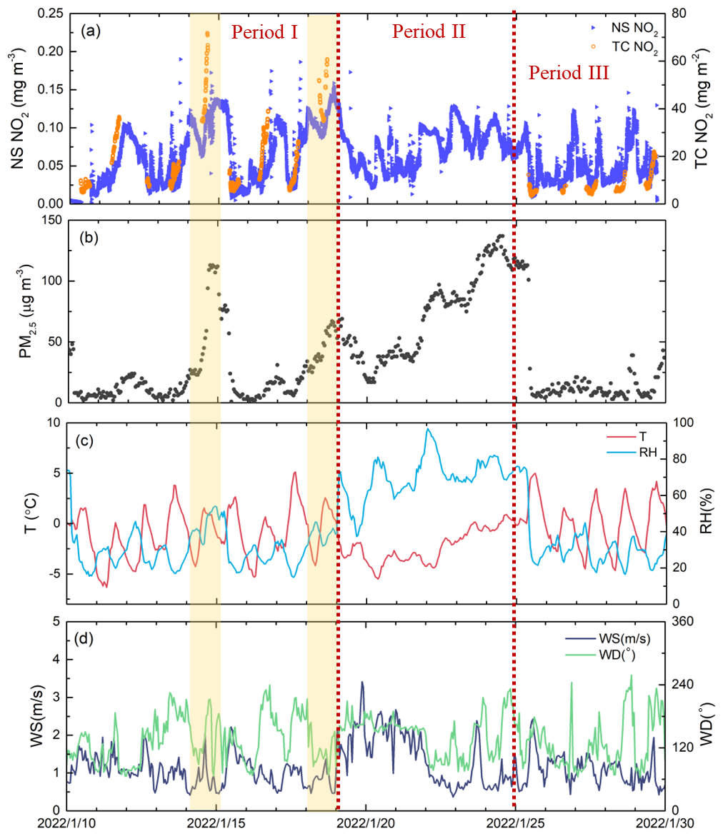
Figure 2 Time series of observed parameters from 10 to 29 January 2022, (a) total VCD and NS concentrations of NO₂, (b) NS PM_2.5 concentration, (c) temperature and relative humidity, and (d) wind speed and wind direction from WMO meteorological station 54511 in Beijing. The vertical dotted lines mark the boundaries between the three periods, and the yellow shaded rectangles mark the two cases discussed in Sect. 3.2.

The time series of the NS PM_2.5 concentrations in Fig. 2b shows four peaks in Period I, with maximum values during the night and very low concentrations (< 10 µg m⁻³) during daytime. The maxima were relatively low on 12 and 17 January (∼ 25 µg m⁻³), whereas on 14 and 18 January the PM_2.5 peak concentrations were ∼ 120 and ∼ 70 µg m⁻³. During Period II, the PM_2.5 concentration increased steadily from less than 25 µg m⁻³ on 20 January to more than 125 µg m⁻³ on the 24th, with similar day/night variations as in Period I. During Period III, the PM_2.5 concentrations were relatively low (< 25 µg m⁻³), and there was no clear diurnal variation.

The air temperature and relative humidity (RH) during the study period are presented in Fig. 2c, and the wind speed and wind direction are presented in Fig. 2d. During Period I, air temperature, RH, and wind speed all varied strongly with a clear diurnal pattern: elevated wind speed during the day, with daily maxima between about 7 and 13 m s⁻¹, and very low wind speed during the night (< 2 m s⁻¹); daytime air temperatures around 0 °C and nighttime temperatures around −10 °C; dry air during the day (RH ∼ 20 %) and more humid during the night (RH of 60 %–80 %). The wind was mostly from northerly directions (NW–NE) and veering during the night. During Period II, the air temperature increased gradually from about −5 to about 0 °C, with small diurnal variations, and relative humidity (RH) increased initially from 40 % to 60 % on 20 January and then gradually to about 70 %, with little day/night variations. During the nights of 22–25 January, the humidity was very high, and the RH sensor saturated and reported maxima close to 100 %. Wind speed during this period was low (< 3 m s⁻¹), and wind direction was mostly SE. During Period III, day/night temperature and RH fluctuations occurred, with daytime air temperatures above 0 °C and gradually rising and RH varying between 20 % during the day and 60 % during the night. Wind speeds were higher during the day, mostly a little higher than 3 m s⁻¹, than they were during the night (close to 0 m s⁻¹), and wind direction was mostly northerly.

The variations of the NO₂ and PM_2.5 concentrations were similar in the sense that the minimum and maximum peak concentrations occurred at about the same time, but with differences in the ratios between minima and maxima. The occurrence of peak concentrations during the night is consistent with the variation in meteorological conditions, with maxima during low wind speed and low air temperature, conducive to the formation of a nocturnal boundary layer in which the concentrations accumulate near the surface. This is observed during Periods I and III. During Period II, however, there were no Pandora observations during daytime due to the occurrence of clouds. This suggests that clouds may also have been present during the night. Hence, radiative cooling was reduced, and air temperature did not decrease as much as during the other periods. Wind speed was low, so pollutants were not transported away and accumulated in the area, as also indicated by the high RH. Hence, the concentrations of NO₂ and PM_2.5, as well as RH, gradually increased during Period II, with relatively small diurnal variations.

For further analysis, we selected two cases for which both total VCD and NS concentrations of NO₂ data were available, including lidar observations and air mass trajectories. The selected cases are the periods when both NO₂ and PM_2.5 concentrations were high, i.e., on 14 and 18 January, when the 24 h average NO₂ concentrations exceeded 80 mg m⁻³. The first pollution episode (case 1) started in the afternoon of 14 January and ended in the morning of 15 January. The other pollution episode with high NS NO₂ occurred on 18 January (case 2). The diurnal variation of the NS NO₂ concentrations was similar in both cases, while the air temperature, RH, wind speed, and wind direction showed that the meteorological situations were similar. However, differences are observed in the temporal variations of total VCD of NO₂ concentrations versus NS NO₂ concentrations and in PM_2.5 concentrations.

3.2 Variations of total VCD and NS concentrations of NO₂ during the two selected cases

Many studies (Yin et al., 2025; Dong et al., 2020; Chang et al., 2019; Li et al., 2017) indicated that the pollution in Beijing mainly originates from three pollution transport patterns: southwest (SW), southeast (SE), and south mixing (SM) patterns. Among them, the most representative are the SW transport path from Shanxi Province to Shijiazhuang–Baoding–Beijing and the SE transport path from Shandong province to Cangzhou–Langfang–Tianjin–Beijing. However, few studies have explored the vertical transport of pollution types. Cases 1 and 2 are representative of the widespread SW and SE patterns, respectively. The processes influencing the concentrations are identified based on lidar data, providing information on the boundary layer structure, together with large-scale weather maps and air mass trajectory analyses, providing information on sources of pollutants and their transport over a wider area. Our study primarily focuses on the correlation between total VCD and NS concentrations of NO₂. Total VCD of NO₂ is provided by the passive remote sensing instrument Pandora, which does not provide reliable observations on cloudy days, as mentioned above. This is the reason why we only selected cases during Period I and did not obtain cases during Period II, when pollution was more severe.

3.2.1 Case 1: disconnected boundary layers merging (14 January 2022)

Time series of the total VCD and NS concentrations of NO₂ on 14 January 2022 (Fig. 3a) show their different evolution throughout the day. NS concentrations showed diurnal variation, decreasing from midnight (0.11 mg m⁻³) to the morning (0.065 mg m⁻³ at 10:30), followed by an afternoon increase and strong evening fluctuations (0.04–0.175 mg m⁻³), likely associated with rush hour emissions and domestic heating. During the limited observation window (10:30–15:30) for Pandora, both VCD and NS concentrations initially showed similar behavior with minimal variation. However, their temporal patterns diverged after 13:00, while NS concentrations plateaued, VCD exhibited rapid growth (40 to 72 mg m⁻² between 12:00 and 15:00), nearly doubling before declining slightly. The difference in the temporal behavior between the total VCD and NS concentrations of NO₂ is amplified in Fig. 3b, which shows a scatterplot between the total VCD and NS concentrations. Observations before and after 13:00 are plotted with different symbols and are color coded in blue and red, respectively. For each of these two data sets, before and after 13:00, VCD and NS concentrations are well correlated with linear correlation coefficients R of 0.94 and 0.85, respectively, but with significantly different slopes.

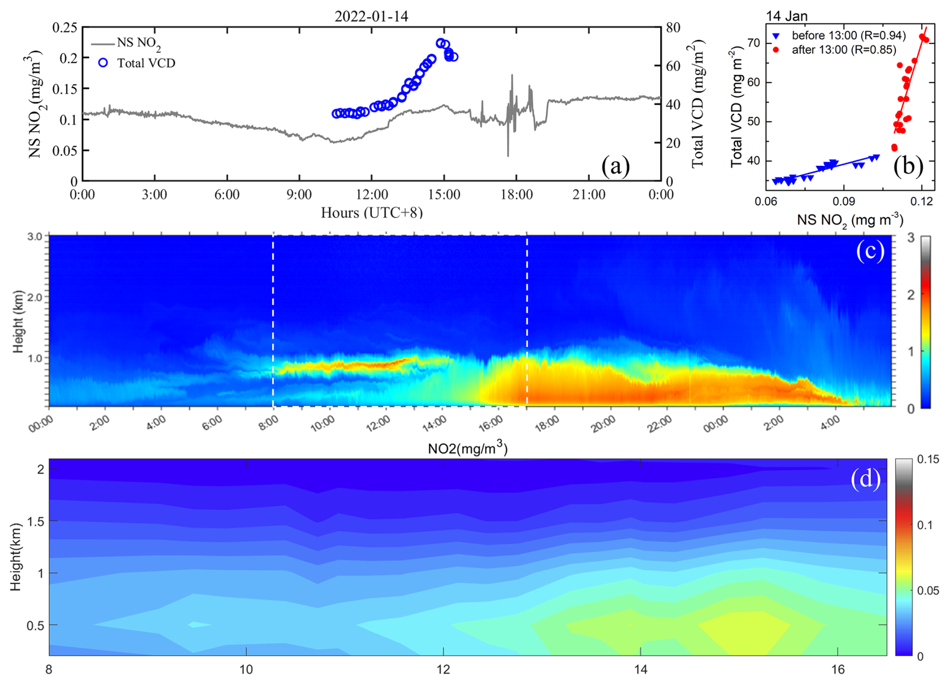
Figure 3 (a) Time series of NS NO₂ (gray line) and total VCD of NO₂ (blue circles) at the Beijing-RADI site (40.004° N, 116.379° E) on 14 January 2022; (b) scatterplots of total VCD and NS concentrations of NO₂ and fits to these data during the morning (before 13:00) and during the afternoon (after 13:00), showing different relationships as discussed in the text; (c) time series of vertical profiles of range-corrected lidar signals at 1064 nm. Note that the lowest height in panel (c) is 100 m; (d) time series of NO₂ vertical profiles derived from Pandora sky radiance measurements. Note that the Pandora profiles are constructed from layer-averaged volume mixing ratios interpolated to six standard levels, and the lowest level is 0.2 km.

The different behavior of the total VCD and NS concentrations of NO₂ can be explained by considering the dynamical behavior of the boundary layer structure. Lidar observations reveal the vertical structure of the atmospheric boundary layer from the variation of the lidar signal as a function of height. A 3-D plot of the vertical variation of the lidar signal, measured on 14 January 2022 at the Beijing-RADI site, close to the Pandora and the ground-based measurements, is presented in Fig. 3c. The lidar signals are color coded according to the scale to the right of Fig. 3c, and each vertical line shows the variation of the lidar signal with height, plotted along the primary vertical axis. The time of measurement of each profile is plotted along the horizontal axis. The lidar signal in this figure is range-corrected, i.e., corrected for attenuation as the laser light propagates in the atmosphere away from the emitter and, after backscattering by aerosol particles, back to the receiver. The time between emission of the laser pulse and receiving the backscattered signal is a measure of the height where the backscattering takes place (after correction of the slant to a vertical optical path), and the intensity is a measure of the aerosol concentration.

The lidar observations in Fig. 3c revealed a complex boundary layer structure with distinct aerosol layers. The data show a well-mixed shallow boundary layer between midnight and 03:00 and the formation of an internal boundary layer after about 04:00, disconnected from the layer above. The internal boundary layer rises gradually until about 11:00 (up to about 400 m), with the clean layer above (between 400 and 500 m), and a new layer (at heights of approximately 800 to 900 m) appears around 07:00, probably due to advection. This vertical variation indicates a disconnected boundary structure with two disconnected layers, likely caused by nocturnal cooling (Stull, 1988). The temperature gradient prohibited material exchange between these layers, leading to the accumulation of near-surface emissions and the trapping of trace gases and aerosols in the upper layer. The occurrence of such a situation is consistent with the observations discussed in Sect. 3.1 and Fig. 2, with low wind speed, lowest air temperature during Period I (−12 °C), and enhanced RH (indicating trapping of water vapor together with decreased air temperature). Note that wind direction was southeasterly during a short period of time on 14 January with a wind speed of 2 m s⁻¹, slightly more than during the rest of the day when the wind direction was northerly. During southeasterly winds, polluted air may be advected to the Beijing-RADI site, whereas during northerly winds, clean air is advected (Liu et al., 2024).

The lidar data in Fig. 3c show that after 12:00, the lower layer deepened and backscatter was observed from the clean layer, indicating that aerosol was gradually mixed into that layer, which completely disappeared around 14:00. At the same time, the lidar signal from the growing lower layer increased gradually, whereas after 13:00 the lidar signal from the upper layer became smaller, indicating that the aerosol concentration decreased until both layers were mixed around 14:00 into a well-mixed boundary layer. After 15:00, the lidar signal increased, first near the surface and then growing throughout the boundary layer. The increase in the NS concentrations (Fig. 3a) is consistent with the highest PM_2.5 concentrations as presented in Fig. 2b and the overall increase in the lidar signal, indicating increasing aerosol concentrations. This is confirmed by AERONET aerosol optical depth (AOD) observations at the Beijing-RADI site (https://aeronet.gsfc.nasa.gov/cgi-bin/data_display_aod_v3?site=Beijing_RADI&nachal=2&level=2&place_code=10, last access: 18 April 2025), which, however, were only available until 16:00 LT.

The vertical variation of the NO₂ concentrations, derived from the Pandora sky radiance measurements at four elevations, is presented in Fig. 3d. Pandora data are only available during daytime, and therefore only the period from 08:00–16:30 can be shown. The NO₂ concentrations are available in four layers. Assuming that NO₂ is uniformly distributed within each layer, the data were interpolated to form a time series of NO₂ vertical distributions, similar to the lidar profiles. The data in Fig. 3d show the similar behavior of the NO₂ concentrations and the aerosol backscatter, with increasing concentrations between 12:00 and 17:00 and their vertical mixing. In particular, the increase around 15:00 is evident in both the Pandora and lidar observations. However, the Pandora observations do not show the occurrence of disconnected boundary layers in the morning. Instead, the Pandora observations show an enhanced layer between 300 and 800 m, rather than the more detailed structure visible in the lidar data. These differences stem from the difference in vertical resolution between the Pandora and the lidar: the total VCD from Pandora is divided into two layers (approximately 300–800 and 800–1700 m) within the detailed stratified height range (300–1000 m) observed by the lidar. Consequently, the fine stratified structure within 1000 m cannot be identified with the available Pandora data.

The overall similarity between the variations in the lidar and Pandora observations supports the use of lidar observations to explain the dynamic behavior of the NO₂ concentrations. In particular, the different relations between total VCD and NS observations before and after 13:00 (Fig. 3b) can be explained by the occurrence of disconnected layers. The variations of the NS NO₂ concentrations until 13:00 reflect the effects of chemical processes and emissions within the atmospheric layer near the surface and within the elevated layer where only removal processes influence the NO₂ concentrations. As a result, the temporal variation of the concentrations in both layers was in part influenced by the same processes, differences were not large (Fig. 3a), and the relationship between the total VCD and NS concentrations was linear with a small slope (174.24) and a strong correlation (R = 0.94) (Fig. 3b). In the afternoon, such processes resulted in the increase in NO₂ concentrations, but when the two layers connected and the wind speed increased somewhat (Fig. 2c, d), NO₂ was mixed throughout the whole boundary layer up to about 1000 m. Hence, the usual afternoon increase in NO₂ concentrations near the surface (Liu et al., 2024) was offset by upward transport, distributing the NO₂ across the whole boundary layer and thus enhancing the total VCD. This is well illustrated by the time series of both NC and total VCD between 13:00 and 15:00 (see Fig. 3a). As a result, the relationship between total VCD and NS changed substantially after 13:00 (Fig. 3b).

The effect of transport on the NO₂ concentrations at the Beijing-RADI site on 14 January 2022 was analyzed using the data presented in Fig. 4: the spatial distribution of tropospheric NO₂ columns derived from TROPOMI data (overpass time 13:30), the synoptic weather map at 00:00 UTC, and 24 h backward trajectories for arrival at the Beijing-RADI site at altitudes of 300, 500, and 1000 m at 10:00, 13:00, and 16:00 LT. The TROPOMI data show the relatively high tropospheric NO₂ concentrations over the study area, in particular over an elongated area stretching from the SW to the NE over Hebei Province, including Beijing (compare with Fig. 1), and from Beijing eastward. This area is bounded by the Taihang mountains in the west and by the Yan mountains in the north, blocking transport of pollutants. The weather map in Fig. 4b shows the pressure distribution and location of low pressure areas resulting in wind from the SW, i.e., along the direction of the elongated area with elevated NO₂ concentrations (see Fig. 4a). This is confirmed by the air mass trajectories in Fig. 4c, all showing overall transport from the SW. However, the trajectories arriving at 10:00 LT show that, during the last 8 h, the air mass arriving at 300 m came from the NE at low wind speed, and the air mass arriving at 500 m came from the NW at even lower wind speed. The air mass arriving at 1000 m came from the SW during the last 14 h before arrival and from the NW during the earlier 12 h. The air masses arriving at 13:00 show similar trajectories. These trajectories are consistent with the lidar observation of disconnected layers, with different air mass trajectories during the last hours before arriving at the Beijing-RADI site and thus possibly different compositions. The air mass arriving at 1000 m had been at high elevations during its entire 24 h trajectory and originated from altitudes higher than 1500 m, but those arriving at 300 and 500 m originated from the surface at different locations separated by tens of km and may thus have been influenced by different sources.

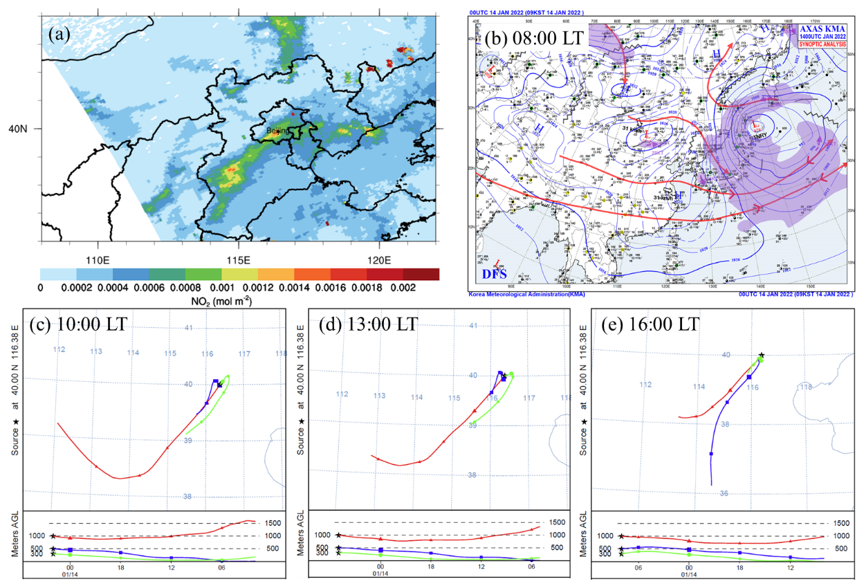
Figure 4 (a) Spatial distribution of tropospheric NO₂ in the study area derived from TROPOMI data on 14 January 2022. (b) Synoptic weather map at 00:00 UTC (08:00 LT); (c–d) 24 h backward air mass trajectories arriving at the Beijing-RADI site at 10:00 (c), 13:00 (d), and 16:00 LT (e) at heights of 300, 100, and 1000 m, calculated using the HYSPLIT model with 6 h time steps (00:00, 06:00, 12:00, and 18:00) and a shorter time step up to the arrival time.

3.2.2 Case 2: multi-layer structure on 18 January 2022

Time series of the total VCD and NS concentrations of NO₂ on 18 January 2022 are shown in Fig. 5a, together with a scatterplot between the total VCD and NS concentrations in Fig. 5b and 3-D plots of the vertical variation of lidar backscatter coefficients in Fig. 5c and Pandora-derived NO₂ concentrations in Fig. 5d. The observational data for 18 January reveal distinct diurnal patterns in NO₂ dynamics, with NS concentrations exhibiting higher baseline levels than those on 14 January, while following a similar initial decreasing trend until 11:30. Subsequently, NS concentrations demonstrated nonlinear growth, plateauing at 0.12 mg m⁻³ (about 1 h after 14:30) before further increasing to 0.16 mg m⁻³ by 21:00, attributed to combined rush-hour emissions and reduced photochemical dissipation. Concurrently, total vertical column density (VCD) displayed accelerated morning depletion (from 54 to 36 mg m⁻³ between 08:30 and 12:30), but, in contrast to the 14th, after 11:30, the total VCD of NO₂ concentrations continued to decrease while the NS NO₂ concentrations increased. Hence, in this situation, it may be difficult to determine NS NO₂ concentrations from the relationship (R = 0.40) before 13:00 (Fig 5b). After 13:00, the total VCD of NO₂ increased from about 37 mg m⁻² to almost 60 mg m⁻² at 16:30, with a plateau around 15:00, and the scatterplot in Fig. 5b shows a good correlation between TS and NS NO₂ concentrations.

Figure 5 Same as Fig. 3 but for 18 January 2022.

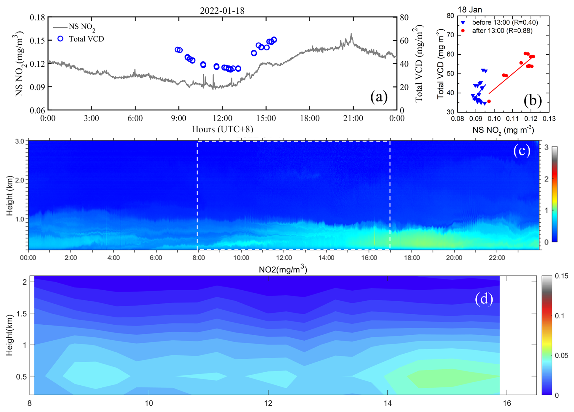
The lidar data in Fig. 5c, with lower intensity than on 14 January, indicate smaller aerosol concentrations on 18 January than on 14 January, consistent with the smaller PM_2.5 concentrations (in Fig. 2b). The lidar data show the occurrence of multiple layers during the night and morning, with sharp boundaries indicating that aerosol particles are trapped in rather shallow layers with little or no exchange between these layers. After 10:30, the boundaries between layers became less sharp, indicating the onset of vertical transport, although the very shallow clear layer (dark blue) between 500 and 600 m indicates a clear separation between the lower and upper layers, prohibiting vertical transport. Around 13:00, this shallow layer disappeared, and after 15:00, the atmospheric boundary layer appeared well mixed up to the top at about 800 m.

The time series of the NO₂ vertical distributions in Fig. 5d shows that NO₂ concentrations were lower on the 18th than on the 14th and were concentrated below 1000 m. The observation of lower concentrations on the 18th and the 14th seems to be in contrast with the higher NS concentrations on the 18th than on the 14th mentioned above. However, the Pandora profiles are constructed from layer-averaged volume mixing ratios interpolated to six standard levels, and the lowest level is 0.2 km. Hence, in view of the layered structure on the 18th, the higher NS concentrations may be disconnected from the lowest layer set at 0.2 km. It is further noted that the Pandora vertical distributions show lower NO₂ concentrations on the 14th than on the 18th in the morning, whereas they are higher in the afternoon of the 14th. The NO₂ concentrations and their vertical distributions varied between 08:00 and 12:30, with an initial increase between 08:00 and 10:00, with a broad elevated maximum centered around 500 m, and another small maximum around 11:00. Apart from these, the NO₂ concentrations were rather homogeneously distributed up to the top of the atmospheric boundary layer at about 800 m, as also indicated by the lidar data. After about 12:00, the NO₂ concentrations increased with a significant enhancement after 14:00.

The evolution of the atmospheric boundary layer, as shown in detail by the lidar data, and the variation of the NO₂ concentration profiles provide a plausible explanation for the evolution of the total VCD and NS concentrations of NO₂ and their ratios, with changes around 11:30 and 13:00. The plateau in the NS NO₂ concentrations may be indicative of the dilution near the surface due to upward transport and vertical mixing, at the same time increasing the TS NO₂ concentrations.

Figure 6 shows the large-scale situation for the study area on 18 January. The TROPOMI data in Fig. 6a show the spatial distribution of the tropospheric NO₂ VCDs, which are highest to the SE of Beijing, in Hebei/Tianjin and over the Yellow Sea. Over Beijing, the tropospheric NO₂ VCDs, as indicated by TROPOMI, are substantially lower than in case 1. This can be explained by the transport from clean areas to the west and west-northwest of Beijing, as indicated by the air mass trajectories arriving in Beijing at 300, 500, and 1000 m at 10:00, 13:00, and 16:00 LT (Fig. 6c). The trajectories of the air masses arriving at 10:00 LT show a clear difference between the lower and higher layers visible in the lidar data: the air arriving at 1000 m originated from the WNW and had traveled during the last 24 h over clean areas (Fig. 6a) over a distance of 1000 km (10°), between heights of 1000–1500 m, while the lower air mass was influenced by local air from SSW (at 300 m) and SW (500 m) that had traveled during the last 24 h near the surface at heights up to 500 m over moderately polluted areas. Hence, the lidar data show higher aerosol content in the lower layer (< 500 m) than in the layer above (> 600 m), and both disconnected layers originated from different origins.

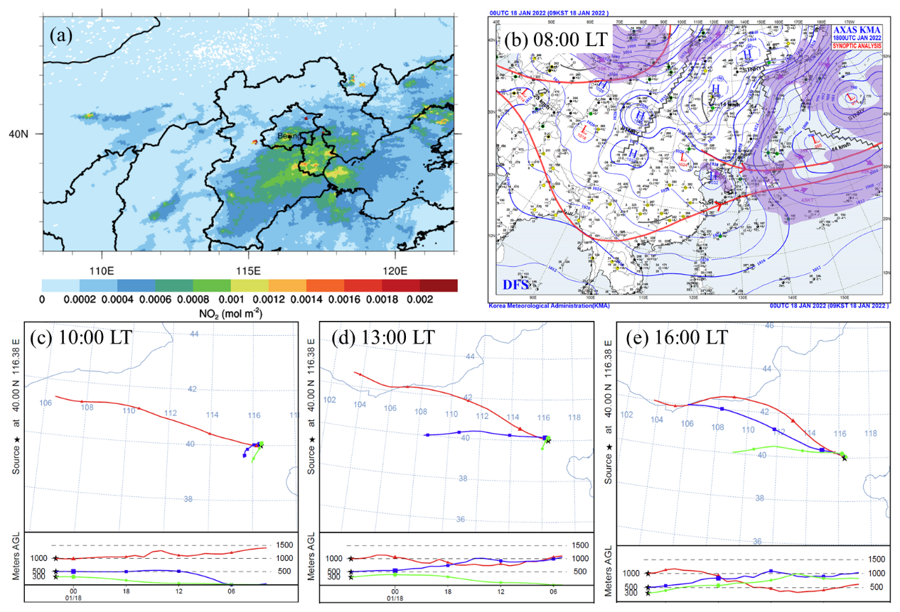
Figure 6 Same as Fig. 4 but for 18 January 2022.

This situation changed as indicated by the air mass trajectory arriving at 13:00 LT. The air mass arriving at 300 m had the same characteristics as at 10:00 LT, had traveled an even shorter distance, and the layer adjacent to the surface was more stagnant. However, the air mass arriving at 500 m now came from the west, had traveled over clean areas (Fig. 6a) at heights between 500 and 1000 m, and thus was distinctly different from the layer below. The air mass arriving at 1000 m originated from a bit further north and further away (in Inner Mongolia) than at 10:00 LT and had traveled at heights between 750 and 1000 m. Hence, all three air masses suggest that the layers originated from different regions and likely had different compositions.

The trajectories of the air masses arriving at 16:00 LT indicate that the situation had changed, i.e., the pollution episode was finished, and pollution was replaced with cleaner air transported from the W to WNW over distances of hundreds of km, originating from elevations of 500–1000 m for air masses arriving at 300 and 500 m, whereas the air mass arriving at 1000 m had actually followed a lower trajectory.

A comparative analysis of the two cases reveals distinct characteristics. Case 1, on 14 January, is characterized by a belt-shaped pollution event. The air mass arriving at 1000 m was primarily transported from Shanxi to Beijing, arriving from the SW during the last 15 h (Fig. 4c), while at lower levels the air masses traveled at low altitudes (from near the surface to 500 m) through the polluted area in Hebei (compare Fig. 4a and c). In contrast, case 2, on 18 January, was a large-scale pollution event covering Shandong, Hebei, Henan, and the southern part of Beijing (Fig. 6a), but the air mass arriving at 1000 m had been transported from the WNW over a large distance over clean areas. However, at lower levels, the air was stagnant (wind speed was low) in the morning; air masses arriving at 300 and 500 m at 10:00 LT had traveled over very short distances during the last 24 h and were thus only influenced by local pollution. In case 1, elevated pollutant concentrations were recorded in the 800–1000 m altitude layer in the morning, attributable to an air mass originating from Shanxi Province (with no significant pollution observed there) that was transported over the polluted area in Hebei at about 1000 m (Fig. 4a and c), and the upper-level air mass likely carried pollutant residuals that had been uplifted through vertical mixing processes over the polluted area in Hebei. These pollutants were subsequently advected to Beijing, where their presence was detected by lidar observations. Conversely, in case 2, pollutants were predominantly transported from the plains, leading to a significant accumulation of pollutants in the near-surface layer. After 13:00, in both cases, the distinction between the pollutant layers disappeared when the boundary layers developed under the influence of surface heating and increasing wind speed (Fig. 2), thus creating boundary layer turbulence and mixing of NO₂, aerosols, and other constituents. Both the total VCD and NS concentrations of NO₂ increased, with that of total VCD of NO₂ being more significant. This further suggests that it is more difficult to obtain NS NO₂ concentrations using total VCD of NO₂ concentrations during the morning hours. However, utilizing the types of pollution spatial distribution and transport patterns can be helpful in indicating NS NO₂ concentrations.

3.3 Ratio of total VCD versus NS NO₂

The two pollution cases discussed above show that the ratio between total VCD and NS concentrations of NO₂ in the morning (before 13:00) is different from that in the afternoon (after 13:00) during the study period in the winter in Beijing. In order to better understand the relationship between total VCD and NS concentrations of NO₂, we calculated their ratio for each day, while we also differentiated between the morning and afternoon using 13:00 as the split time. The ratio of total VCD to NS NO₂ concentrations serves a dual purpose: it not only quantifies the changes between total VCD and NS concentrations of NO₂ when the correlation is low but also reflects the degree of dispersion between the two measurements. A more variable ratio indicates higher dispersion and poorer correlation, providing a straightforward yet effective way to assess the reliability of using total VCD of NO₂ to predict NS NO₂ concentrations.

The results are presented as violin plots in Fig. 7, for each of the 12 d for which data are available. The data in Fig. 7 show that the mean and median values of the NO₂ ratio during Period I (10–18 January) were substantially higher than those during Period III (25–30 January), with the exception of 25 and 29 January. These 2 d, at the beginning and end of Period III, signify the transition from polluted to clean days (see Fig. 2b). On most days, the ratio was smaller in the morning than in the afternoon. The difference between the morning and afternoon ratios was small during the 2 d (14th and 18th) with accumulated pollution, while during the 4 d, when wind speed increased on 13th, 15th, and 17th, the differences were relatively large, with the largest difference of 192 m on the 13th. During Period III, the difference between the morning and afternoon ratios was basically smaller than 50 m, with a gap of more than 100 m only on the 29th. There were no valid observations of total VCD of NO₂ during Period II, so it is not possible to judge the changes in ratio over multiple consecutive days of pollution. Throughout the observation period, the standard deviations of the ratios were overall larger in the morning than in the afternoon, when the winter boundary layer was well mixed and the relationship between total VCD and NS concentrations of NO₂ was relatively stable. However, in the morning, when the boundary layer was developing, the day-to-day variations in the standard deviation imply relatively large changes in the ratio. The box plot in Fig. 7b illustrates the difference between the morning and afternoon ratios. The mean values are lower in the morning (364 m) than in the afternoon (428 m), and the upper quartile in the afternoon is closer to its median value, suggesting that the ratio is more stable in the afternoon when it is well mixed vertically. However, although the ratio is quite stable in the afternoon when the boundary layer is generally well mixed, there are still unpredictable extreme values (e.g., 771 m).

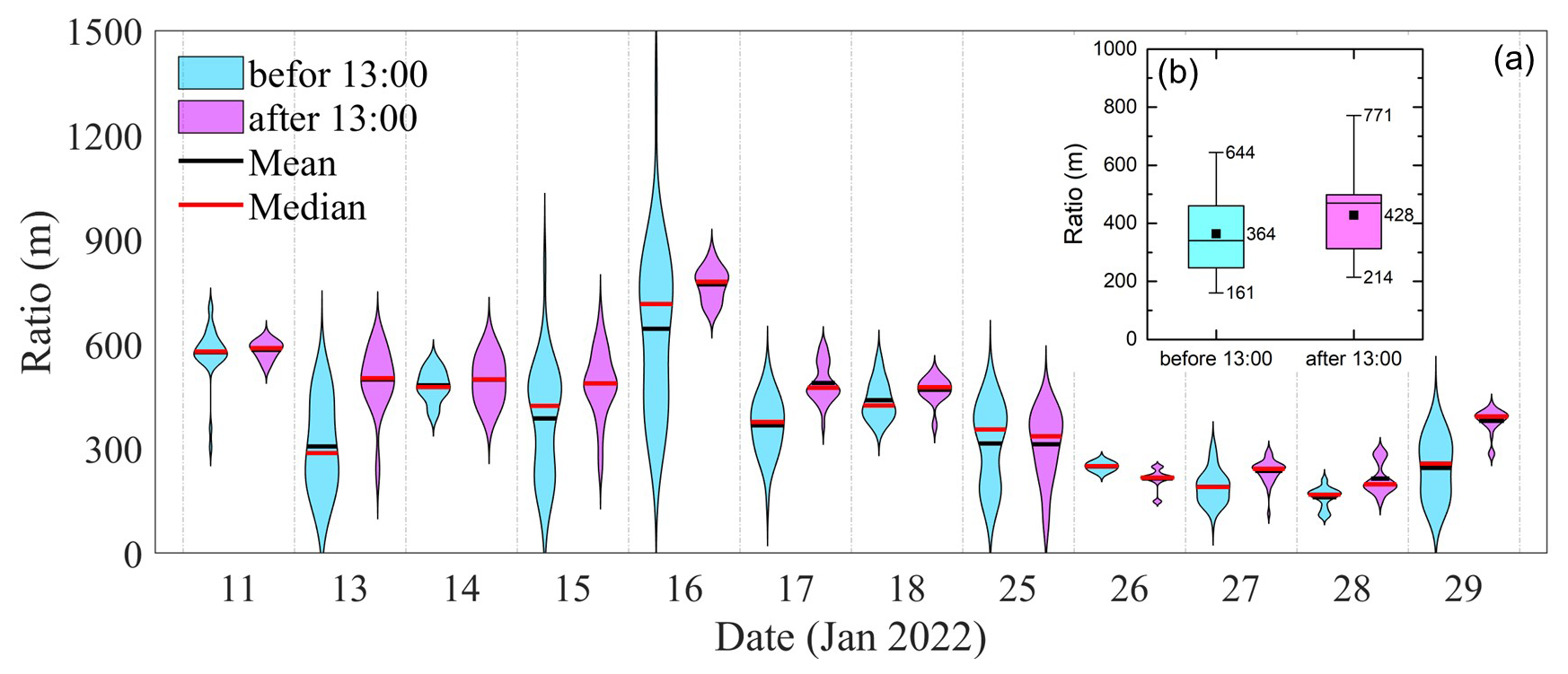
Figure 7 (a) Violin plots of the ratio of total VCD and NS concentrations of NO₂ for each day when observations were available in January 2022, where the data were differentiated between the morning (before 13:00 LT) and the afternoon (after 13:00 LT). (b) The box-whisker plot of the ratio averaged over all observations before and after 13:00 LT in January 2022. The horizontal lines in the boxes and the top and bottom edges represent the mean and upper and lower quartile values of the ratio, respectively; the solid square dots represent the median values, and the bars represent the minimum and maximum values.

Generally, the temporal stability of the ratio is important. The ratio is overall less variable after 13:00, suggesting that polar-orbiting satellites can be used to predict NS NO₂ based on total VCD of NO₂ during this period with greater confidence. This temporal stability is particularly valuable because it offers a feasible approach for air quality monitoring and forecasting. In contrast, the ratio is less stable before 13:00, posing greater challenges for using geostationary satellites for the same prediction task. It is worth noting that our analysis of winter in Beijing suggests that considering both the spatial distribution of pollutants and their transport direction has the potential to enhance the ability of satellites to predict NS NO₂ concentrations based on total VCD of NO₂. By incorporating this information into prediction models, the accuracy and reliability of satellite-based air quality predictions may be improved, particularly in complex urban environments where pollutant concentrations can vary significantly over short distances and time periods.

4 Discussion and conclusions

Total column and near-surface NO₂ data observed during the winter field experiment from 10 to 29 January 2022 at the Beijing-RADI site were analyzed together with lidar, PM_2.5 and meteorological data, satellite data, weather maps, and air mass trajectories. Based on these observations, the experimental period was subdivided into three periods: intermittent pollution days, persistent pollution days, and clean days. The analysis of the total VCD and NS concentrations of NO₂ shows substantial differences between the first and third periods, while during the second period, with persistent pollution, no total VCD of NO₂ observations were available due to the presence of clouds. During the first period, two episodes with high pollution were identified and analyzed in detail with a focus on the ratio between the variation of the total VCD and NS concentrations of NO₂ and their ratio. The relations between the total VCD and NS concentrations of NO₂ in the morning and in the afternoon, split at 13:00 LT, appear to be significantly different. These differences have been explained in terms of boundary layer dynamics, using lidar data showing the vertical stratification with disconnected boundary layers at different heights in the morning, which connected as the boundary layer developed in the afternoon. In addition, the four-layer NO₂ column concentrations obtained from Pandora show good agreement with the lidar signal in terms of the temporal and vertical variations of the NO₂ concentrations, with differences attributed to the different vertical resolutions of the Pandora and lidar observations, as well as the physical properties of NO₂ and aerosols. From this, together with air mass trajectories, weather maps, and TROPOMI satellite observations of the NO₂ spatial distribution, a consistent picture was created showing different source regions for disconnected air masses arriving at different heights and different times of the day.

Data from the full experimental period, with 12 d for which valid data are available, were analyzed in detail to obtain more insight into the variation of the ratio between the total VCD and NS concentrations of NO₂. This ratio appears to be overall smaller in the morning than in the afternoon, with larger standard deviations. In addition, the ratios and their standard deviations were overall larger during the more polluted episode I than during the relatively clean Period III.

Daytime continuous remote sensing observations of Pandora were used in this study, and the results confirm its possible importance in understanding changes in the distribution of NO₂ in the vertical direction. The NO₂ vertical distribution has been analyzed using less than 3 weeks of observation data, which has some limitations, but the research idea is worthy of reference and promotion. In the future, the implementation of larger-scale experiments in different typical regions and seasons will help to provide further understanding of the ideas presented in this study and improve the shortcomings. Moreover, we will broaden the scope of experimental areas and field sites to complement research on the various pollutant emission and transport characteristics. Furthermore, observations over a longer period will allow us to capture more representative cases, thereby enhancing the reliability of our findings.

The overall conclusion from this study during a relatively short period of almost 3 weeks in the winter in Beijing is that the variation between the total column and near-surface NO₂ concentrations varies with the concentration level and the time of day. In the afternoon, the boundary layer is well developed and satellite observations are sensitive to the NS concentrations, whereas in the morning this depends on meteorological conditions. Hence, satellites with an afternoon overpass are capable of measuring total VCD of NO₂ that is representative of NS concentrations, whereas observations earlier in the day may not be. This could possibly affect the interpretation of diurnal variations derived from observations using geostationary satellites.