Adjustments to an abrupt solar forcing in the CMIP6 abrupt-solm4p experiment

“Radiative” or “rapid” adjustments refer to the response of the climate system to an instantaneous radiative forcing, independent of surface temperature changes. These adjustments occur over timescales from hours (e.g. aerosol–cloud interactions) to months (e.g. stratospheric temperature changes), often overlapping with feedback mechanisms – making their separation in realistic scenarios challenging. Controlled simulation experiments can thus help isolate adjustment processes and improve understanding relevant to more complex cases like volcanic eruptions or ongoing climate change.

The abrupt-solm4p experiment of the Cloud Feedback Model Intercomparison Project (CFMIP), part of the 6th Coupled Model Intercomparison Project (CMIP6), simulates an instantaneous 4 % reduction in the solar constant from a pre-industrial state on 1 January 1850. This study analyses changes in climate variables, cloud properties, and radiative fluxes across different timescales (hours, days, months and up to 150 years) to identify adjustment mechanisms and characteristic fingerprints for a shortwave forcing scenario.

The four participating models show rapid adjustments of $\mathrm{3.57}\pm \mathrm{0.46}\mathrm{W}{\mathrm{m}}^{-\mathrm{2}}$, offsetting ∼ 35 % of the initial forcing. Distinct local patterns include initial rapid surface cooling – especially over Antarctica and the Southern Hemisphere. Stratospheric cooling slows the polar night jet, disrupts the polar vortex, and increases Arctic cloud cover, causing local warming. Within the first month, the troposphere cools more quickly than the ocean surface, decreasing vertical stability and enhancing cloud cover over oceans, while tropical land regions show the opposite change. On monthly timescales, high clouds shift downward due to reduced convective heating.

1 Introduction

The Earth's climate is governed by radiative fluxes entering and leaving the atmosphere. In a steady-state system, incoming and outgoing fluxes are balanced, maintaining an equilibrium of the Earth climate system. In the case of any perturbation to this balance, known as a radiative forcing, the climate system reacts by heating or cooling, which leads to a new balance of energy fluxes on timescales of centuries. Different processes in the climate's response, called feedbacks or adjustments, either enhance or dampen the Earth's capability to reach a new equilibrium. Feedbacks act in response to global mean surface temperature change and typically take place over years and centuries. In contrast, adjustments happen in direct response to a forcing agent, are independent of surface temperature change, and mostly evolve on shorter timescales of days, weeks and months (Andrews and Forster, 2008; Gregory and Webb, 2008; Sherwood et al., 2015). Radiative adjustments of the atmosphere to an external forcing are of particular interest to the scientific community, and a growing number of studies have been conducted on the subject (Gregory et al., 2004; Zelinka et al., 2013; Myhre et al., 2013; Sherwood et al., 2015; Smith et al., 2018; Forster et al., 2021b; Quaas et al., 2024). By introducing radiative adjustments into the forcing-feedback framework as part of the effective radiative forcing (ERF;  Myhre et al., 2013), the resulting ERF is a better predictor of implied global surface temperature change, since it is more independent of the kind of forcing agent (Andrews and Forster, 2008; Gregory and Webb, 2008). However, this approach requires a precise estimate of ERF, which comprises the instantaneous radiative forcing (IRF) as well as (radiative or rapid) adjustments (RAs), which are prone to high uncertainty, especially in the case of cloud adjustments (Andrews and Forster, 2008).

The total global mean radiative imbalance at the top of atmosphere (TOA) $\overline{N}\left(t\right)$ can be written as

$$\begin{array}{}\text{(1)}& \overline{N}\left(t\right)=\mathrm{IRF}+\mathrm{RA}+\sum _i{\mathit{\lambda }}_i\mathrm{\Delta }\overline{T}\left(t\right),\end{array}$$

where the sum over the feedback parameters λ_i accounts for the different sources of feedbacks.

Although RAs are formally independent of global mean surface temperature change, local temperature changes and consequential atmospheric adjustments can contribute a considerable amount to the overall RA (Quaas et al., 2024). Furthermore, despite many adjustments happening on timescales from hours to days (e.g. precipitation and changes in some cloud properties), adjustments of the stratosphere, cryosphere or vegetation can take months to years (Forster et al., 2021b; Stjern et al., 2023). This leads to an overlap of adjustment and feedback timescales, which makes it difficult to disentangle both. Moreover, adjustments are often confounded by climate variability in magnitude, making it very hard to detect them in observations. This is further complicated by the transient nature of most forcing processes happening in the Earth climate system, like the gradual increase in CO₂ from anthropogenic sources in the atmosphere.

To circumvent these issues, climate models allow the application of instantaneous forcings that exceed climate variability and are kept constant, facilitating a better analysis of adjustments and feedbacks. A common experiment using global climate models is the instantaneous 2- or 4-fold increase in the atmospheric CO₂ concentration (e.g. Gregory et al., 2004; Colman and McAvaney, 2011; Kamae and Watanabe, 2012; Zelinka et al., 2013; Andrews et al., 2015) in order to predict long-term consequences of anthropogenic climate change as well as short-term adjustments.

However, these simulations are often highly idealised, using fixed sea surface temperatures (SSTs) or omitting the existence of continents (aqua-planet simulations). In order to compare and validate such results with observations, a natural forcing is required that is applied nearly instantaneously and is of sufficient strength. Volcanic eruptions are considered such so-called “natural laboratories” (e.g.  Malavelle et al., 2017; Christensen et al., 2022). Large volcanic eruptions emit huge amounts of aerosols into the atmosphere in a very short time frame of hours. If transported up to the stratosphere, depending on the location and season of the volcanic eruption, the aerosol can form a global scattering layer with a lifetime of up to 1 to 3 years (Myhre et al., 2013). This way, volcanic eruptions exert a radiative forcing that is approximately comparable to the instantaneous forcing that usually only models can realise. However, examining volcanic eruptions includes other challenges. The initial forcing is very localised, and only after a few months is the aforementioned scattering layer formed around the globe. Depending on the location of the volcano, the strength of the manifold adjustment mechanisms and the distribution of the stratospheric aerosol layer vary. Hence, timescales of different adjustments might still overlap. Therefore, before analysing adjustments to a realistic volcanic eruption, it can be helpful to further simplify the problem. A reduced solar constant forcing can serve as a simplified analogue to a stratospheric volcanic aerosol layer, as both reduce the amount of shortwave radiation reaching the troposphere.

In this study, we thus examine the results of the abrupt-solm4p experiment, which is part of the Cloud Feedback Model Intercomparison Project (CFMIP) as part of the 6th Climate Model Intercomparison Project (CMIP6) (Eyring et al., 2016; Webb et al., 2017). The output of four global climate models, which participated in this experiment, is available. In the simulations the solar constant was reduced by 4 % and kept constant at this value. This can be regarded as a simplified analogue for an aerosol scattering layer. Volcanic eruptions and a reduced solar constant both lead to a reduced incoming shortwave flux at the surface, even if stratospheric adjustments are expected to differ. Hence, similar adjustment patterns are expected for both types of forcing, when the scattering sulfate layer distributes over the whole globe with time.

There have been numerous studies that analysed the reaction of the Earth climate system to a number of different forcing agents so far (e.g.  Gregory et al., 2004; Smith et al., 2018). However only few studies quantified radiative adjustments after solar forcing and took a closer look at the specific processes happening in response (e.g. Salvi et al., 2021; Virgin and Fletcher, 2022; Aerenson et al., 2024). Radiative adjustments to solar forcing in sum typically counteract the initial forcing (e.g. Smith et al., 2018; Russotto and Ackerman, 2018; Virgin and Fletcher, 2022; Aerenson et al., 2024). Most of this is attributed to decreased temperature of the troposphere, stratosphere and land surface, which leads to a reduction in longwave radiation lost to space. The effect is partially offset by the reduction in water vapour in the atmosphere, following the Clausius–Clapeyron relationship, and thereby an increase in outgoing longwave radiation. Moreover, Smith et al. (2018) find a positive adjustment due to change in surface albedo. Furthermore, differential heating of sea and land surface can lead to changes in circulation patterns, which affects precipitation and cloud properties. On longer timescales also a change in vegetation might happen, but this is not subject of this study, and no further analysis was performed here.

However, when analysing rapid adjustments due to changes in cloud properties, the studies find contradictory results. This is in accordance with an overall high uncertainty linked to cloud property changes in climate models. Reducing short-term uncertainty of cloud adjustments could also reduce uncertainty of long-term predictions (Andrews and Forster, 2008; Nam et al., 2018). In the case of solar forcing, Smith et al. (2018) and Virgin and Fletcher (2022) find cloud adjustments that counteract the initial solar forcing. In response to a +2 % solar constant forcing, Smith et al. (2018) describe an increase in cloud fraction in the boundary layer, a reduction in the cloud fraction in the free troposphere, a small increase in cloud fraction at around 100 hPa and a decrease above this level. This is very similar to our findings, although of the opposite sign, since we examined the response to a reduction in the solar constant. Using radiative kernels, Smith et al. (2018) show that cloud changes lead to negative long- and shortwave effects but with high model disagreement in the shortwave effects. In response to a +2 % solar forcing, Virgin and Fletcher (2022) find that the shortwave component is dominated by changes in the boundary layer clouds, while changes in the troposphere contribute more to the longwave effects. In contrast to this, Aerenson et al. (2024) find cloud adjustments that further amplify the initial solar forcing. In response to a +4 % solar constant forcing, they find an overall positive cloud radiative adjustment, which is strongest where the low-cloud fraction is reduced. The two main mechanisms are changes in cloud fraction and cloud optical depth, which they find are of opposite sign in the case of solar forcing. Moreover, short- and longwave effects tend to partially compensate for each other, but shortwave effects are slightly stronger. Hence, in total, positive shortwave effects due to decreased cloud fraction dominate the overall cloud adjustments. However, they find that the participating models do not agree on the signs of cloud adjustment effects, and the uncertainty of the total effect is high.

Even though the studies describe similar changes in cloud properties, the derived cloud radiative adjustments differ depending on the applied method and models used. This demonstrates how radiative effects of cloud property changes are still one of the major sources of uncertainty in climate models, even in highly idealised solar forcing scenarios. Hence, this study is particularly interested in adjustments of cloud properties and characteristic patterns in response to shortwave forcing.

CFMIP provides outputs from the +4 % solar constant (solp4p) as well as the −4 % solar constant (solm4p). Using both experiments would increase the amount of data statistics could be based on. However, as, for example, Aerenson et al. (2024) found, response to positive and negative solar forcing does not only differ in sign but also shows different patterns due to non-linearities and dependence on the base state. Hence, for this study, we decided to only look at rapid adjustments to a reduction in solar constant (solm4p), which in a later step could be compared to adjustments to volcanic forcing.

Reduced solar constant simulations are also of interest for the increasing number of solar radiation modification (SRM) studies that often aim to balance the forcing due to anthropogenic emissions of CO₂ by reducing the absorbed solar radiation (e.g. Bala et al., 2008; Cao et al., 2015; Schmidt et al., 2012; Huneeus et al., 2014; Russotto and Ackerman, 2018). Not only having a better understanding of the long-term effects of SRM methods, but also knowing about short-term adjustments can improve the risk assessment of these endeavours. In these scenarios, not only the global mean evolution of climate variables, but also, if not even more, local processes are of high importance. Especially short-term adjustments of clouds and precipitation can lead to local droughts or floods, with possibly important effects for local communities.

There are several methods to quantify radiative adjustments in climate models. On the one hand, the linear regression method (Gregory et al., 2004), based on Eq. (1), allows for a simultaneous quantification of ERF, equilibrium climate sensitivity (long-term trend) and climate feedback parameter (∑λ_i). In order to derive radiative adjustments from ERF, knowledge of the instantaneous forcing is necessary. For most forcing agents, it is possible to diagnose the IRF by separate radiative transfer modelling. However, the regression method is only feasible for the global mean, and it relies on the assumption that all rapid adjustments happen while the global mean surface temperature change is still zero. This is an oversimplification, as inert systems like cryosphere or vegetation might still adjust to the initial forcing, while global mean surface temperature has already begun to change.

On the other hand, the fixed surface temperature method (Hansen et al., 2005) or rather fixed sea surface temperature (fixed-SST) is widely used and has the advantage of suppressing feedbacks (Forster et al., 2016). This allows for the disentanglement of adjustments and feedbacks. However, this method artificially suppresses adjustments of ocean surface temperature and introduces unrealistic land–sea contrast, which hinders a realistic estimate of circulation adjustments. Andrews et al. (2021) showed a significant difference in ERF depending on whether only sea surface temperature or all surface temperature was kept at zero. Possible adjustments to localised warming or cooling cannot be simulated in this kind of setup, although in some concepts they are considered adjustments relevant to TOA ERF (Quaas et al., 2024).

The simulations analysed in this study apply an instantaneous solar forcing that is kept constant, while allowing the whole climate system to adapt in a fully coupled general circulation model. The regression method was used to quantify ERF and RA, but non-linear behaviour was found for the first 4–10 years, when the more inert systems like ocean, cryosphere or vegetation still adjust to the forcing, while global mean surface temperature change starts to dampen TOA radiative budget imbalance. Nevertheless, this model setup allows us to examine adjustment processes on timescales of hours, days and months, where, as we show, TOA radiative budget change is still dominated by adjustment processes rather than temperature-mediated change.

Section 2 contains a more detailed description of the experiment setup as well as an overview of the available data. Section 3 first shows the results of the classical regression method by Gregory et al. (2004), in order to quantify ERF and RA. It then discusses how timescales of hours, days and months are dominated by adjustment processes and examines TOA radiative fluxes and cloud radiative effect (CRE) anomaly. Afterwards, it proceeds with a closer analysis of adjustment processes of a number of different climate variables. These include surface and atmospheric temperature, relative humidity, vertical velocity, and cloud fraction. Section 4 discusses the results of this study in the context of studies that have been conducted on adjustments to solar forcing in recent years and discusses the limitations of the dataset and the approach. Section 5 contains a summary and provides an outlook on how this study's findings can contribute to future research in the field of radiative adjustments.

2 Methods

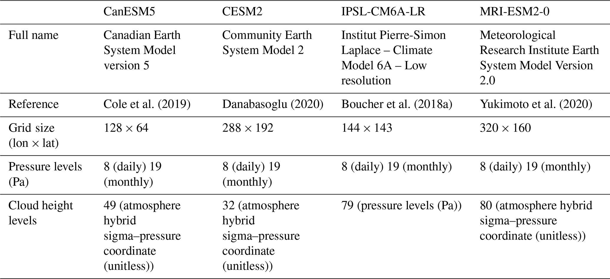
In the solm4p-experiment, the solar constant is reduced instantaneously by 4 % and kept constant at 96 % of the solar constant of the pre-industrial control run (piControl). It branches off the piControl simulation on 1 January 1850. No other forcing is considered in the experiment. The diagnostics of four models, which participated in this experiment, are available: IPSL-CM6A-LR, CESM2, CanESM5 and MRI-ESM2-0 (further information provided in Table 1). For each model, one experiment run corresponding to one piControl run is provided (IPSL-CM6A-LR, Boucher et al., 2018b; CESM2, Danabasoglu et al., 2019; CanESM5, Swart et al., 2019; MRI-ESM2-0, Yukimoto et al., 2019). While some models provide 3-hourly output for several parameters, CESM2 only provides daily data. In the case of vertically resolved atmospheric cloud fraction, only monthly data were available from all four models. More information on the four models, including their horizontal and vertical grid spacing, is provided in Table 1.

Cole et al. (2019)Danabasoglu (2020)Boucher et al. (2018a)Yukimoto et al. (2020)

Table 1 Information on the four models for which output was available from the CFMIP abrupt-solm4p experiment.

For all variables examined in this study, the difference attributable to the reduction in solar constant was calculated for each parameter by subtracting the piControl run from the solm4p run for each point in time and space.

Following Stjern et al. (2023), four different timescales were considered: the first 100 h, the first 30 d, the first year and the following years until 150 years after the onset of forcing. For the first timescale (up to 100 h) 3-hourly data were used, when available, otherwise daily data were used. For the second timescale (days 5–30) daily averages were used, for the third timescale (months 2–12) monthly data were used and for the long-term development (years 2–150) yearly means were plotted. The transitions between the plots of different timescales often display a small jump because the next frequency does not contain the last data point of the preceding frequency but an average.

For all timescales the global mean was calculated for each model. Moreover, a multi-model mean was calculated by first interpolating all models to the time axis of the MRI-ESM2-0 model. This model was chosen as reference because it provided the most extensive database for the abrupt-solm4p experiment. If not all models provided data of the same frequency, the highest available resolution was plotted for each model, respectively, and for the multi-model mean, the other models were interpolated to the 3-hourly time axis of MRI-ESM2-0.

In addition to the temporal development of global means, a geographical distribution of the respective parameter was plotted, averaging over the respective timescales. For the mean of the first three timescales, all time steps were averaged, while for the fourth timescale only the years 120–150 after the onset of forcing were averaged to obtain an estimate for the long-term new approximate equilibrium state. For the global distribution, a multi-model mean was calculated by interpolating the other models to the CanESM5 horizontal grid, which was the coarsest out of the four models.

Besides the grid spacing, also the height levels varied between the models in the case of the atmospheric cloud fraction data. For the other climate variables, all models used the same 19 height levels. In the case of cloud fraction, the other models were interpolated to the CanESM5 pressure axis.

In order to account for uncertainty, the multi-model standard deviation was plotted together with the temporal development of the multi-model global mean. In the case of global distributions of anomalies, areas were dotted in which fewer than three of four models agreed on the sign of anomaly.

To analyse differences in land and sea surface response, some climate variables, e.g. relative humidity, were averaged only over ocean and only over land. This was done by applying a land–sea mask, based on the CanESM5 grid, before performing the zonal averaging.

This study focuses on cloud adjustments and the cloud radiative effect, which was calculated from the difference between simulation runs with clouds (all-sky) and a second radiative transfer calculation for each step without clouds (clear-sky), both provided by each of the four models. Then, the total cloud radiative effect anomaly at TOA was calculated as the combined effect of solar (shortwave) and terrestrial (longwave) radiation changes due to cloud changes.

The linear regression method introduced by Gregory et al. (2004) was applied for a number of TOA fluxes, in order to estimate their influence on the overall ERF. For that purpose, the yearly global mean of the respective TOA flux change was plotted over the yearly global mean of near-surface temperature change and a linear regression was used, which determined the intercept with the TOA flux axis.

3 Results

In order to estimate the rapid adjustments to a 4 % solar constant reduction, we applied the regression method developed by Gregory et al. (2004) to the solm4p-CFMIP data. The results are shown in the following section. We then move on to examine different timescales after the onset of forcing and investigate how the first three timescales (hours, days and months) are dominated by rapid adjustments, while the fourth timescale shows the long-term adaptation and is therefore dominated by surface-temperature-mediated processes. Afterwards, we analyse the response of different climate variables like temperature, humidity and cloud fraction on the different timescales and identify characteristic adjustment patterns of these variables.

3.1 Effective radiative forcing and rapid adjustment estimate

We applied a linear regression to the yearly global means of TOA radiative budget change (Δ TOA budget or N following Eq. 1) and near-surface temperature change (ΔT) of the four available models. The results are shown in Fig. 1.

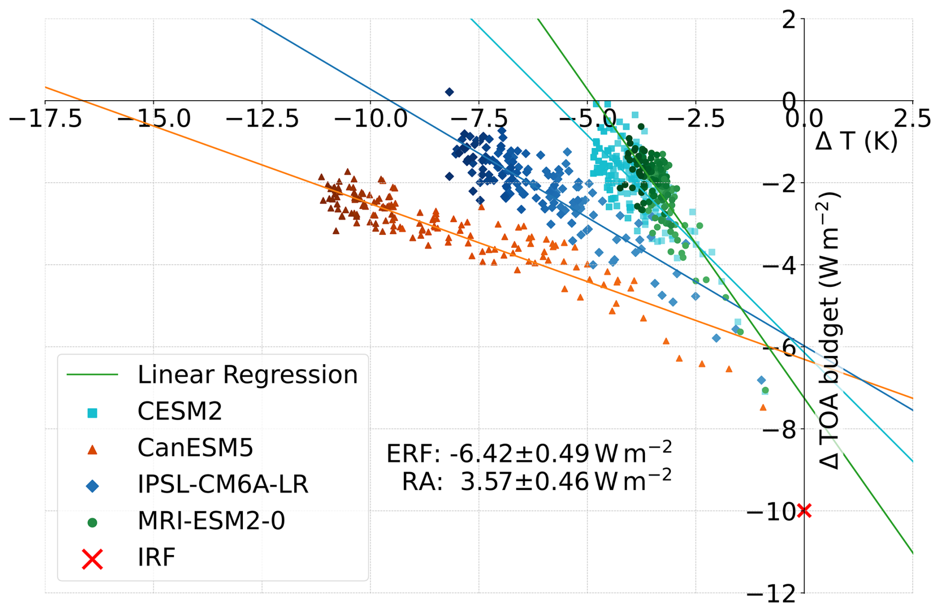
Figure 1 Linear regression plots for yearly global mean TOA radiative budget anomaly in W m⁻² vs. change in yearly global mean surface temperature (ΔT). Increasing saturation of the colours indicates temporal development.

The TOA radiative budget anomaly shows the expected behaviour for all four models, starting with negative values for ΔT=0 and then approaching a new radiative balance. The multi-model-mean IRF was estimated as the difference between the downward and upward shortwave anomaly for the first month after the onset of forcing (shortest output frequency available for all models). The intercept of the linear regressions with the y axis provides the ERF, and the difference between ERF and IRF yields the RA. Multi-model-mean ERF and RA are given at the bottom of the figure and are also provided in Table 2. The negative IRF of approximately $-\mathrm{10}\mathrm{W}{\mathrm{m}}^{-\mathrm{2}}$ is reduced by radiative adjustments of 3.6 W m⁻², resulting in an ERF of $-\mathrm{6.4}\mathrm{W}{\mathrm{m}}^{-\mathrm{2}}$. While some models, like CanESM5 and IPSL-CM6A-LR, simulate a strong temperature decrease in response to the radiative forcing, CESM2 and MRI-ESM2-0 reach a new equilibrium at a significantly weaker change in surface temperature.

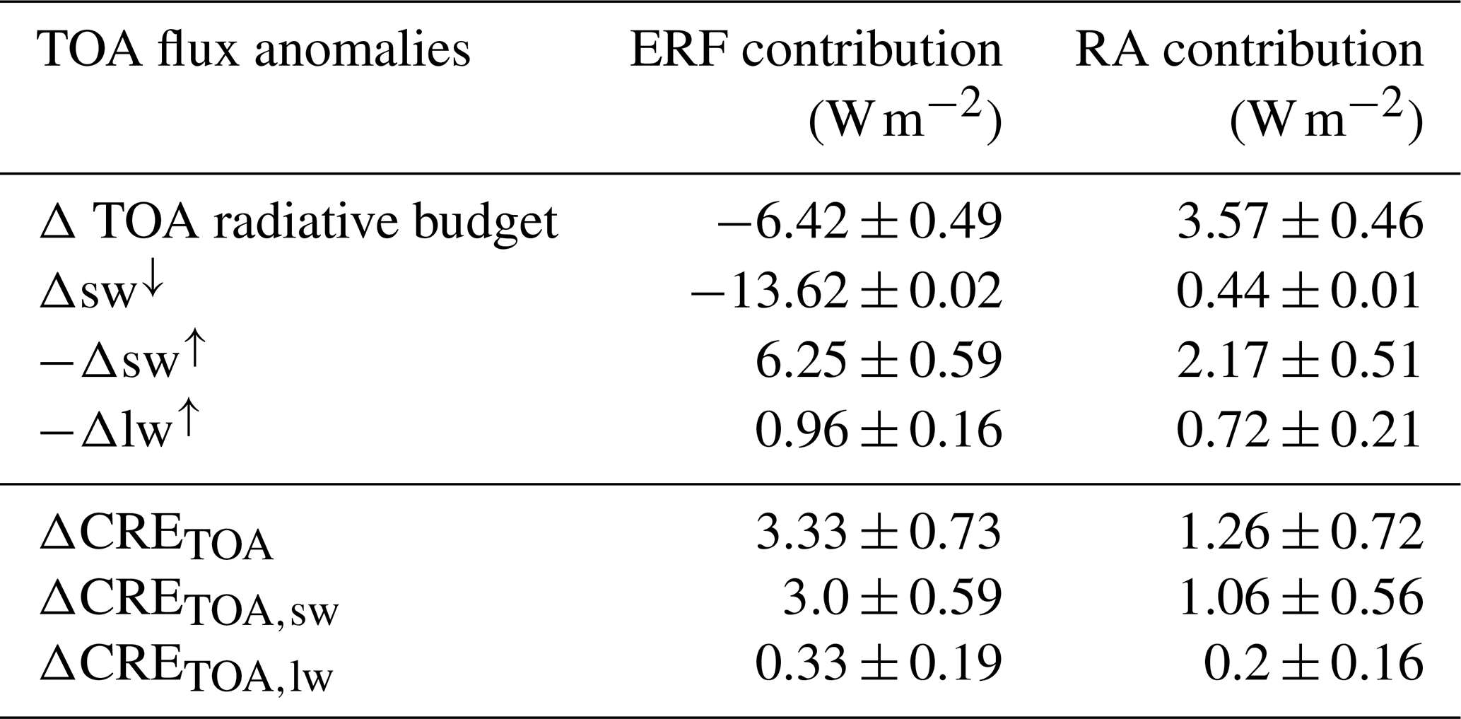
Table 2 Multi-model-mean intercepts of different TOA fluxes derived via the regression method (ERF contribution in W m⁻²) and its deviation from the initial response (RA contribution in W m⁻²) calculated as the difference between the linear regression intercept and the first-month response (∼ IRF contribution).

The development is mostly linear. However, especially for the first 10 years, all models exhibit a slightly steeper slope than in the long term. This deviation could either be interpreted as radiative adjustments developing on timescales as long as a decade, similar to the ocean–atmosphere adjustments found by Rugenstein et al. (2016), or it might suggest a change in the relation between ΔT and N, with the deep-ocean heat uptake starting to dominate the SST pattern after a decade of forcing, changing the overall ocean heat uptake efficacy (Andrews et al., 2015). Other studies like Gregory and Webb (2008) found similar non-linearities and attributed those to shortwave cloud radiative effects. In this study the non-linearity was predominant in the clear-sky shortwave component over ocean, but no further analysis was conducted, as this study concentrates on the adjustment processes during the first year after the onset of forcing.

Analogous to the total TOA radiative budget, linear regressions were also performed for the single components of the TOA budget, i.e. downward shortwave flux change Δsw^↓, upward shortwave flux change Δsw^↑ and upward longwave flux Δlw^↑ (Fig. A1 in the Appendix). Approximating the instantaneous response of the respective radiative components as the offsets after 1 month of simulation, the contributions of the single components to the overall ERF and RA can be estimated and are shown in Table 2. All models simulate an instantaneous response of Δsw^↑ of around $-\mathrm{4.1}\mathrm{W}{\mathrm{m}}^{-\mathrm{2}}$ in reaction to the reduction in the solar constant, depending on the planetary albedo. This is considered to be a part of the IRF, since it is an immediate response to the initial solar constant reduction, not requiring any atmospheric changes. It reduces the negative Δsw^↓ signal by $-(-\mathrm{4.1})\mathrm{W}{\mathrm{m}}^{-\mathrm{2}}$ as IRF and ERF define radiative fluxes positive downwards. However, the $-\mathrm{\Delta }{\mathrm{sw}}^{\uparrow }$ ERF component is 6.3 W m⁻², indicating shortwave radiative adjustments of $\mathrm{6.3}-\mathrm{4.1}=\mathrm{2.2}\mathrm{W}{\mathrm{m}}^{-\mathrm{2}}$. In contrast to that, no longwave contribution to the IRF is expected, and models show no initial response of Δlw^↑. All models simulate a clear linear relationship between Δlw^↑ and ΔT with an intercept of around $-\mathrm{1}\mathrm{W}{\mathrm{m}}^{-\mathrm{2}}$, which, due to sign convention, is equal to a longwave adjustment of 1 W m⁻² at TOA. Hence the longwave component contributes about one-third to the overall RAs, while the shortwave RAs make up the other two-thirds.

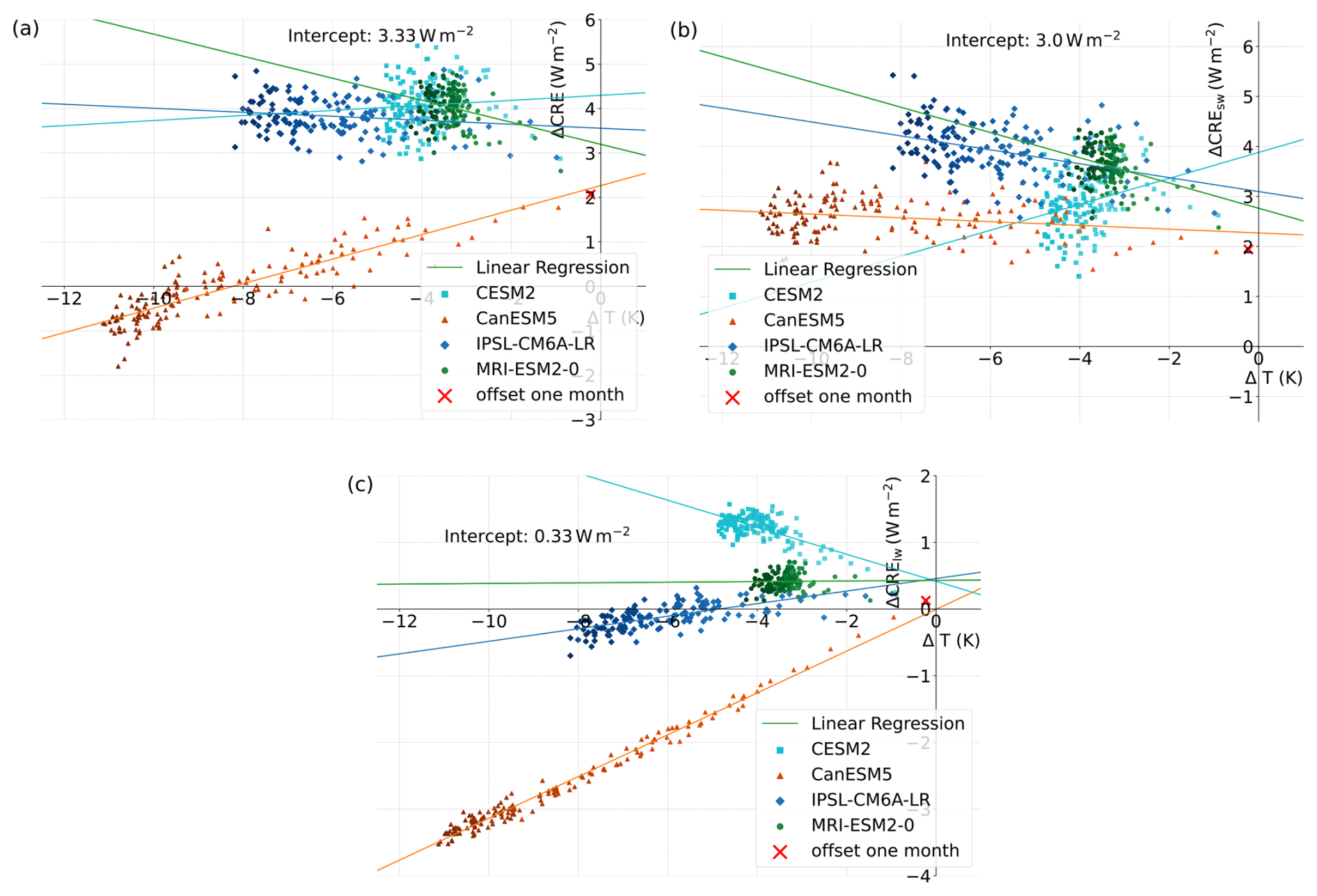
The same method was applied to the cloud radiative effect anomaly (ΔCRE_TOA) and its short- and longwave components (ΔCRE_TOA,sw and ΔCRE_TOA,lw), respectively (Fig. A2 in the Appendix). If an approach similar to the IRF-ERF approach is applied and the initial ΔCRE_TOA is subtracted from the intercept, as it is purely a cloud masking effect, the remaining cloud adjustment is $\mathrm{3.3}-\mathrm{2}=\mathrm{1.3}\mathrm{W}{\mathrm{m}}^{-\mathrm{2}}$, mostly stemming from ΔCRE_TOA,sw, which is a substantial contribution to the overall RA of 3.6 W m⁻². Hence, we find that cloud adjustments counteract parts of the initial solar forcing, as was found by several other studies (Smith et al., 2018; Salvi et al., 2021; Virgin and Fletcher, 2022). The reason for the positive shortwave cloud adjustment found in this study might be the decrease in tropical cloud cover in the boundary layer, as the location of strong positive ΔCRE_TOA,sw (Fig. B2 in the Appendix) often coincides with decreased cloud cover at 850 hPa (Fig. 10). However, our approach does not allow for a quantification of single contributions to the overall cloud adjustments. Moreover, the uncertainty of the cloud radiative effect anomaly is high, and models disagreed on the sign of slope of the linear fits. The intercepts for the cloud radiative effect anomaly and its components are also provided in Table 2.

3.2 Rapid adjustments on different timescales

In the following section we analyse the temporal development of the TOA radiative budget anomaly and its components, as well as of the surface temperature anomaly. The aim is to better understand the contributions of the single components to the total TOA budget anomaly and its interaction with surface temperature change. In contrast to the linear regression method, in this section we look at temporal developments over the first hours, days and months, in order to learn more about the underlying adjustments.

3.2.1 Temporal development of ΔTOA radiative budget and ΔT

Figure 2 shows the global mean of the three components of the TOA radiative budget, downward and upward shortwave flux anomaly (Δsw^↓ and Δsw^↑), and upward longwave flux anomaly (Δlw^↑), together with the TOA radiative budget anomaly. Fluxes are defined positive downwards, so that added up, the three flux anomalies yield the total TOA budget anomaly. Only MRI-ESM2-0 provided TOA shortwave radiative fluxes as daily data, while the other three models only provided monthly data. Hence, Fig. 2 only shows the results of one model for shortwave flux anomalies and the total TOA budget anomaly for the first two timescales. The upward longwave radiative flux was provided as daily output by all models and is plotted accordingly.

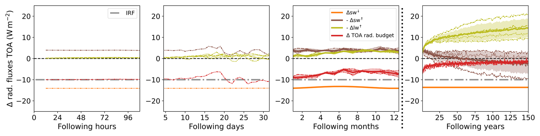
Figure 2 Global mean anomaly of radiative fluxes at TOA in W m⁻² for four different timescales after the onset of forcing (100 h, 30 d, 12 months, 150 years). Plotted are the downward shortwave flux anomaly at TOA (orange), the upward shortwave flux anomaly at TOA (brown), the upward longwave anomaly at TOA (olive) and the radiative budget anomaly at TOA (red). Shading around the multi-model mean shows multi-model standard deviation. If available, the results for all four models (thin lines) were plotted together with the model mean (thick line). In addition to that, the instantaneous radiative forcing (IRF) is plotted as a grey dash-dotted line. Upward fluxes were multiplied by $\cdot (-\mathrm{1})$, such that the three radiative flux anomalies (orange, olive and brown) add up to the TOA radiative budget anomaly (red), which is the same as the black curve in Fig. 4.

Δsw^↓ shows the reduction in the solar constant. It stays constant over all timescales and only displays a yearly periodic deviation due to the elliptical orbit of the Earth around the sun. It is the same for all four models, since the underlying assumption of the abrupt-solm4p experiment is an instantaneous and constant reduction in the solar constant by 4 %, corresponding to a decrease in the downward shortwave flux by $-\mathrm{13}\mathrm{W}{\mathrm{m}}^{-\mathrm{2}}$.

As described before, Δsw^↑ shows an instantaneous reaction, which is part of IRF, since it is a change in TOA radiation in reaction to the forcing, without any changes in atmospheric state. Hence, the IRF is the sum of incoming and outgoing shortwave anomaly at t=0 and is around $-\mathrm{10}\mathrm{W}{\mathrm{m}}^{-\mathrm{2}}$ according to experimental design. Δsw^↑ shows first changes after 10 d, although no clear trend can be recognised. This is a reaction to changes in surface albedo, beginning after roughly 10 d and mostly connected to increased snowfall over land in high northern latitudes and first changes in snow cover and sea ice extent in Antarctica. Furthermore, changes in cloud properties, beginning after a few hours, influence Δsw^↑ over the first month, but there is not one dominating process but rather a complex interplay of mechanisms that result in the global mean temporal change. Over the first year, albedo and cloud properties show significant changes. Nevertheless, the upward shortwave anomaly stays relatively constant, indicating that the different climate variables and local variability approximately cancel out each other's shortwave radiative effects. Over longer timescales, the multi-model mean of upward shortwave flux anomaly decreases, changes its sign around 50 years after the onset of forcing and continues to decrease up until 150 years. However, the individual models do not agree on the sign of the anomaly on these longer timescales. This is due to opposing signs in high latitudes and tropical regions, and the models disagree as to which region dominates the global mean effect (see Fig. B1 in the Appendix). This is a significant difference in the long-term prediction of the models but was not further analysed here, since this study is focused on short-term effects.

In contrast to the shortwave fluxes, there are no immediate effects of the reduction in the solar constant on the Δlw^↑. This is expected because it is closely linked to changes in surface and atmospheric temperature, which need some time to adapt. Similar to Δsw^↑, Δlw^↑ displays the first changes around 10 d after the onset of forcing. It is overall slightly increased over the following days and only temporarily changes its sign. The multi-model mean always stays positive, indicating a reduction in the amount of longwave radiation to space, because the atmosphere and surface reduce their temperature in reaction to the reduced incoming solar energy (the Planck effect). This effect continues, and all models simulate a further increasing Δlw^↑ for longer timescales.

The TOA radiative budget anomaly is overall negative due to the negative forcing and corresponds to the IRF at t=0. It is dominated by the shortwave effects on the timescales of hours and days, but in the course of months, the increasing longwave gain slowly reduces the TOA imbalance until it approaches a new balance over the following decades and centuries.

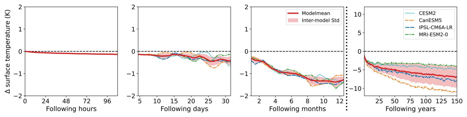
Figure 3 Global mean of near-surface temperature anomaly (in K) for four different timescales after the onset of forcing (100 h, 30 d, 12 months, 150 years). The results of the four participating models are plotted (cyan: CESM2, orange: CanESM5, blue: IPSL-CM6A-LR and green: MRI-ESM2-0) together with a multi-model mean (red, bold) and multi-model standard deviation (shaded area around multi-model mean). For the fourth timescale, the y axis has been adjusted to account for the stronger changes on longer timescales.

Analogous to the TOA radiative flux anomalies, the global mean near-surface temperature anomaly ΔT is shown in Fig. 3. It becomes increasingly negative immediately after the onset of forcing due to decreased absorption of shortwave radiation at the surface. ΔT is of the order of −0.25 K over the first month, continuously decreasing to values $<-\mathrm{1}\mathrm{K}$ after 4 months. The four participating models agree well on the global mean ΔT during the first year but differ in their long-term strength of surface temperature reduction, depending on the model's climate sensitivity.

3.2.2 Simulated vs. calculated ΔTOA radiative budget

In this study, we are interested in rapid adjustments to solar forcing in fully coupled climate models. In those models, the surface temperature begins to adapt from the onset of forcing, leading to a possible overlap of adjustments and temperature-mediated effects (feedbacks).

However, when calculating the TOA budget anomaly N via Eq. (1) by multiplying the ΔT with the feedback parameter λ and adding the ERF, both derived from the linear regression in Sect. 3.1, a significant disagreement between simulated TOA budget anomaly (Fig. 2) and TOA budget anomaly calculated via Eq (1) becomes apparent on the shorter timescales. Figure 4 shows the simulated TOA budget anomaly (N_sim) together with the surface-temperature-mediated TOA budget anomaly calculated from ΔT adding only the IRF (N_calc,IRF) and the complete ERF (N_calc,ERF) for the four different timescales.

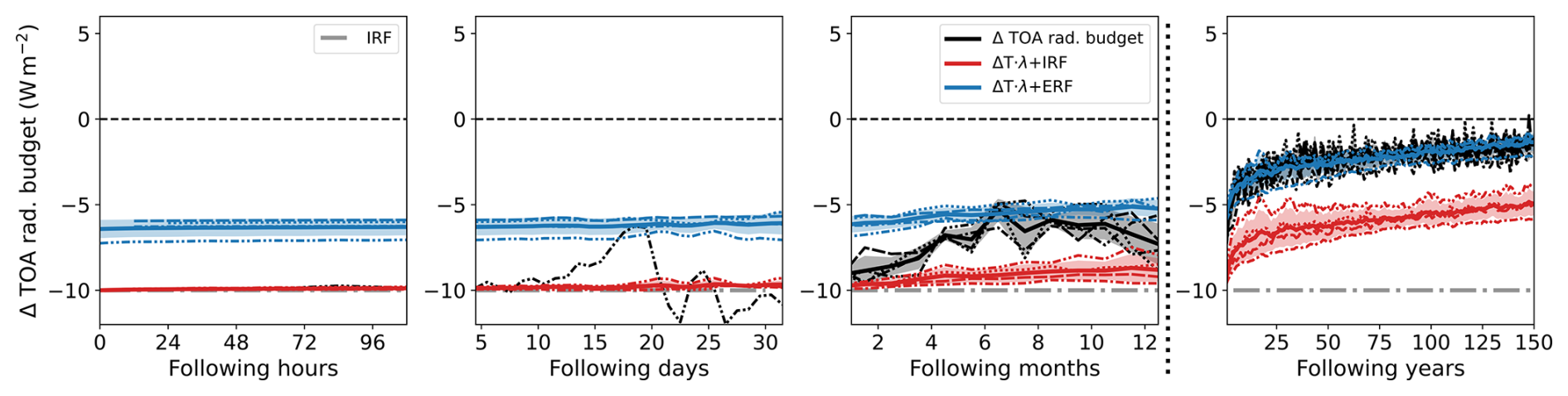
Figure 4 Same as Fig. 2 for simulated and calculated TOA radiative budget changes. Shown are TOA radiative budget change, based on the simulated surface temperature change, only considering IRF (N_calc,IRF, red); the calculated TOA radiative budget change considering $\mathrm{IRF}+\mathrm{RA}=\mathrm{ERF}$ (N_calc,ERF, blue); and the simulated TOA radiative budget change (N_sim, black).

During the first timescale no adjustments or feedbacks take place that would lead to considerable changes in N. Hence, N_calc,IRF and N_sim do not show a strong deviation. However, on all other timescales there is a significant offset between the two. Especially for the timescales of days and months after the onset of forcing, the trend of N_calc,IRF cannot explain the trend of N_sim. For the fourth timescale, both model means show the same trend but with a constant offset, which corresponds to the rapid adjustments (RAs). When adding the RA and IRF yielding N_calc,ERF, the long-term trends of calculated and simulated TOA flux change agree well. However, the first three timescales show considerable deviations between N_sim and N_calc,ERF, and changes in surface temperature are clearly not sufficient to explain the simulated TOA radiative budget variability.

Hence, we argue that the first three timescales are dominated by adjustment processes, while temperature-mediated changes only play a minor part. Clearly, this does not allow for a perfect distinction between adjustments and feedbacks. However, this approach has the advantage that no restrictions have to be made to surface temperature (e.g. fixed-SST experiments), which fail to capture all changes in circulation, and no assumptions are made on the linearity of adjustment processes, as is done in the case of radiative kernels. This study aims to understand changes in the atmospheric state during the first year after the onset of forcing, and based on the beforehand arguments, we assume this timescale to be dominated by adjustment processes.

Unfortunately, only one model (MRI-ESM2-0) provided daily TOA radiative flux data. Therefore, although a deviation of N_sim and N_calc,ERF is clearly visible, a clear attribution to rapid adjustments to the forcing is difficult, as internal variability can also lead to difference between N_sim and N_calc,ERF. However, all models provide data for the following months after the onset of forcing. Although there is some deviation between the models, which is likely caused by internal variability, there is also a common trend (model mean, thick black line), which cannot be explained by the changes in surface temperature or surface albedo (not shown). Instead, adjustments in atmospheric temperature profile, water vapour and cloud properties seem to be the dominating source of variability during the first days and months. Hence, the TOA budget variability is a result of a complex interplay of several atmospheric and cloud variables, with partly compensating effects. Changes in cloud properties have been found to be one of the major sources of model uncertainty on all timescales. Reducing the uncertainty on short timescales would allow for a better quantification of the ERF, thereby improving long-term predictions. Therefore, the aim of this study is to identify characteristic patterns of cloud adjustment in response to a negative shortwave forcing.

The next section analyses the temporal development of the cloud radiative effect anomaly over the three adjustment timescales as well as the fourth timescale, representing the long-term temperature-mediated response. The cloud radiative effect can be an indicator of cloud adjustments, which are a major source of uncertainty in climate models. However, the cloud radiative effect also includes changes in other atmospheric variables (cloud masking), which is discussed in the following section.

3.2.3 Adjustments of the cloud radiative effect at TOA

Figure 5 shows the temporal evolution of the global mean cloud radiative effect anomaly at TOA (ΔCRE_TOA) and its short- and longwave components (ΔCRE_TOA,sw and ΔCRE_TOA,lw). As described before, only MRI-ESM2-0 provided daily data, which are plotted for the first two timescales.

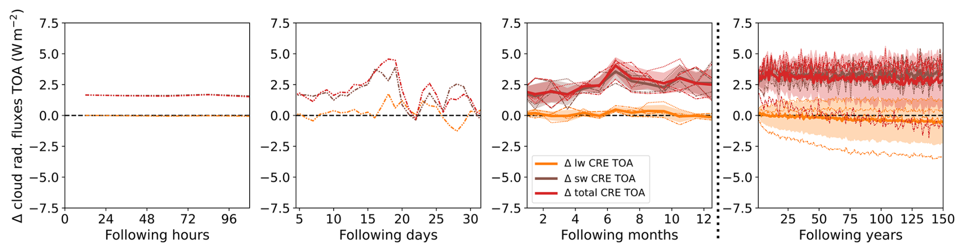
Figure 5 Global mean of TOA cloud radiative effect anomaly (ΔCRE_TOA, red) in W m⁻² for four different timescales after the onset of forcing (100 h, 30 d, 12 months, 150 years). Additionally, shortwave and longwave TOA cloud radiative effect anomalies (ΔCRE_TOA,sw and ΔCRE_TOA,sw) are shown in brown and orange. Their respective intermodel standard deviation is shown as shading around inter-model means.

ΔCRE_TOA is positive for all timescales, indicating a decrease in the generally cooling effect of clouds, partially counteracting the negative forcing. However, since this positive anomaly is apparent from the first time step, the initial value is not attributable to changes in cloud properties. It rather is a result of clouds masking changes in the clear-sky budget. After 5 d ΔCRE_TOA starts to deviate from its initial value and varies with no clear pattern during the first month. During this time period it follows the same shape as the total TOA budget anomaly. Hence, changes in cloud properties seem to be the dominant source of variability of N_sim during the first months. This is supported by the fact that global mean clear-sky fluxes show near to no variability during the first 5 months (not shown). After 6 months, the initial forcing moves from the southern high latitudes to the northern high latitudes. Due to differing surface albedo on the two hemispheres and therefore changes in the clear-sky TOA radiative budget, cloud masking is expected to change at this point.

ΔCRE_TOA further increases over the following years. After about 10 years ΔCRE_TOA remains relatively constant at 4 W m⁻². A slight decreasing trend is visible in the multi-model mean, even though three out of four models simulate a stabilisation of ΔCRE_TOA for longer timescales. This is due to the continuous decrease in ΔCRE_TOA,lw, simulated by the CanESM5 model. Although this model shows the strongest temperature decrease out of the four models, it does not systematically predict the strongest changes in other cloud properties. Hence, the continuous decrease in ΔCRE_TOA,lw likely is a strong cloud masking effect that dominates over any possibly positive ΔCRE_TOA,lw effects due to changes in cloud properties.

ΔCRE_TOA,sw is overall positive on all timescales and dominates ΔCRE_TOA. It seems to be the major source of variability, while ΔCRE_TOA,lw shows no clear sign over the first three timescales and overall less variability than ΔCRE_TOA,sw.

As discussed before, especially signals during the first days will also be influenced by internal variability. However, in the 6th Intergovernmental Panel on Climate Change (IPCC) report, anthropogenic forcing in 2019 was quantified to be of the order of 2.7 W m⁻² (Forster et al., 2021a). Sippel et al. (2021) showed that this allows a robust detection of forced warming, significantly exceeding climate variability. Hence, an instantaneous forcing of $-\mathrm{10}\mathrm{W}{\mathrm{m}}^{-\mathrm{2}}$, which is 4 times stronger, is expected to lead to adjustments that exceed internal variability. Nevertheless, to account for possible effects of internal variability, in the following section on characteristic fingerprints, we only assume a signal to be a rapid adjustment if three out of the four participating models agree on the sign.

3.3 Characteristic adjustment fingerprints in climate variables

The following sections explore the response of surface and atmospheric temperature, as well as relative humidity, vertical velocity and cloud cover, in order to identify characteristic adjustment fingerprints to reduced shortwave radiation availability. Since the global mean TOA budget variability is an effect of a complex interplay of several variables and local effects, the following sections examine global distributions of the variables mentioned before, in order to better understand the underlying mechanisms.

3.3.1 Adjustments of surface and atmospheric temperature

The effects of the reduction in the solar constant are visible in a variety of climate variables already a few hours after the onset of the perturbation.

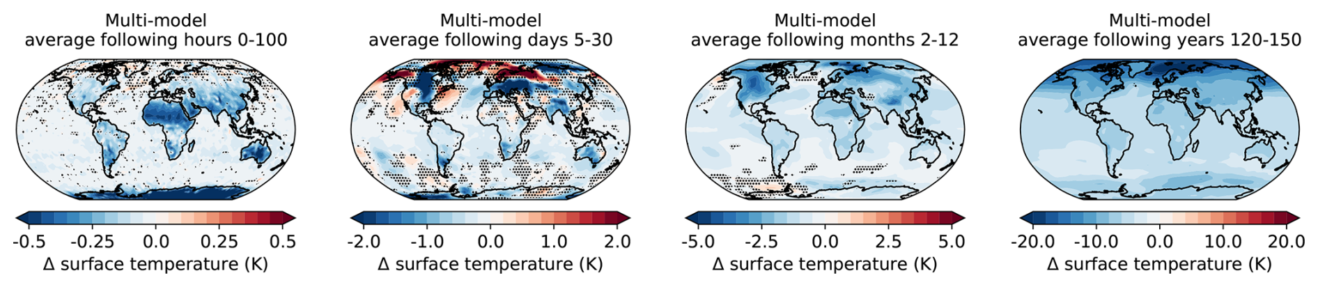
Figure 6 Multi-model-mean global distribution of near-surface temperature anomaly (in K) averaged over four different timescales after the onset of forcing (100 h, days 5–30, months 2–12, years 120–150). The multi-model mean was calculated by interpolating the other models to the grid spacing of the CanESM5 model. Regions where fewer than three of four models agreed on the sign of anomaly are dotted. Note the different scales of the colour bars for better contrast.

Figure 6 shows the geographical distribution of the near-surface temperature anomaly averaged over the first three timescales depicted in Fig. 3 (hours, days and months, respectively) and a fourth timescale averaged over the years 120–150 representing the long-term development.

During the first 100 h the land surface responds to the forcing by cooling down, while the ocean surface temperature stays approximately constant due to its higher heat capacity. The strongest cooling occurs over Antarctica because of the 24 h exposure to solar radiation at time of forcing onset (1 January). Areas of low heat capacity (e.g. Antarctica and Sahara) generally exhibit a stronger surface temperature decrease compared to other regions on the same latitude because the same amount of heat reduction will lead to a stronger decrease in temperature. In contrast to the overall cooling of surface temperature, the Arctic, which does not experience any solar forcing in January, warms up during the first hours and days after the onset of forcing. The reduced temperature gradient between the tropics and the Arctic leads to a reduction in polar night jet strength, which perturbs the polar vortex. Cold-air outbreaks as well as warm-air intrusions result in strong changes of surface temperature over days and the first month. Intrusion of warm, moist air masses into Arctic latitudes increases cloud cover, which reduces the amount of longwave radiation lost to space, leading to local surface temperature rise. However, the individual pattern of surface temperature increase will depend on the base state of the respective model. Hence, although all models simulate an increase in Arctic temperatures, the specific location varies, which leads to higher uncertainty in the Arctic response compared to other regions. Also, the Southern Hemisphere shows a pattern of warming and cooling, though less pronounced, due to the positioning of the forcing.

After 1 year, Arctic amplification begins to emerge as an overall stronger cooling of the surface over Arctic latitudes compared to lower latitudes and Antarctica. The ocean surface starts to cool down, although the decrease is still smaller compared to land surfaces.

The average over years 120–150 shows an overall cooling in all regions. Arctic amplification is apparent as a stronger cooling over Arctic latitudes. North of Antarctica, where sea ice extent is increased compared to the piControl runs, the surface cooling is slightly stronger compared to the land surface of Antarctica, due to more severe changes in surface properties compared to the control run. The differences between land and sea surface are less apparent compared to the shorter timescales because the deeper ocean also adapts to the new energy balance.

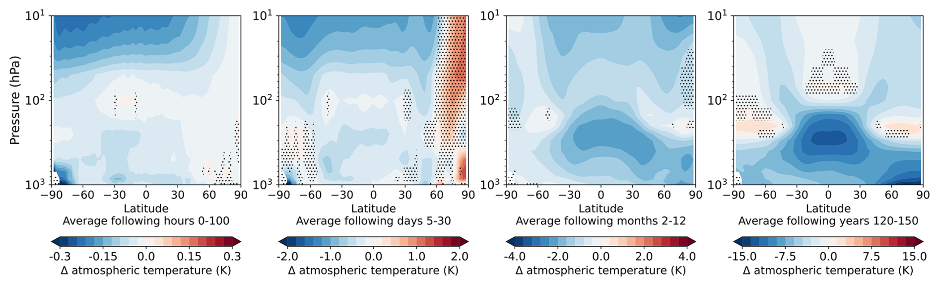
Figure 7 Multi-model mean and temporal and zonal mean vertical profiles of the atmospheric temperature anomaly (in K) as a function of latitude for four different timescales after the onset of forcing (100 h, days 5–30, months 2–12, years 120–150). Regions where fewer than three out of four models agree on the sign of anomaly are dotted. Note the adjusted colour scales for the different timescales.

Figure 7 shows the zonal mean of atmospheric temperature anomaly averaged over timescales of hours, days and months and the years 120–150, respectively.

During the first 100 h, the stratosphere cools down quickly, especially above Antarctica, where the radiative forcing is strongest. Since the stratosphere is nearest to the source of forcing, the cooling of the stratosphere is stronger than the cooling of the troposphere during the first hours and days. The cooling effects are strongest at the highest altitudes, where most of the high-frequency radiation is absorbed.

In the near-surface layers, cooling above Antarctica is further amplified because the surface temperature drops rapidly, which reduces sensible heat flux.

After 1 month, atmospheric temperature change is highly variable in northern latitudes, due to the beforehand described perturbation of the polar vortex. Warm-air intrusions into Arctic latitudes strongly increase the atmospheric temperature in near-surface layers.

Over the first year, the troposphere adjusts to the solar forcing via an overall reduction in tropospheric temperature, especially in the middle and upper troposphere in the tropics. This pattern resembles the long-term climate response, where it contributes to a lapse rate feedback. However, similar atmospheric temperature adjustments have been documented under solar forcing in fixed-SST experiments (e.g. Salvi et al. (2021)). In these experiments, land surface temperatures can still respond, but their change is strongly tied to nearby ocean temperatures through atmospheric coupling. Consequently, this limits any substantial climate feedbacks from developing, leaving predominantly fast adjustment processes. This indicates that the pattern found in this study could be driven by changes in atmospheric absorption, humidity and convection in reaction to the forcing itself, rather than being a surface-temperature-mediated effect. We discuss this point further when analysing the results for humidity and cloud fraction.

On longer timescales the tropospheric temperature continues to decrease. In the tropics this is most pronounced in the higher troposphere, while at high latitudes the cooling is stronger in the lower troposphere because the characteristic atmospheric temperature profiles in these regions react differently to a decrease in surface temperature. In higher latitudes, the tropopause descends. Hence, the stratospheric vertical increase in temperature starts at lower altitudes, which manifests as a warming at 200 hPa at the poles. At ±30°, the stratosphere cools at all pressure levels.

3.3.2 Adjustments of humidity, vertical velocity and cloud fraction

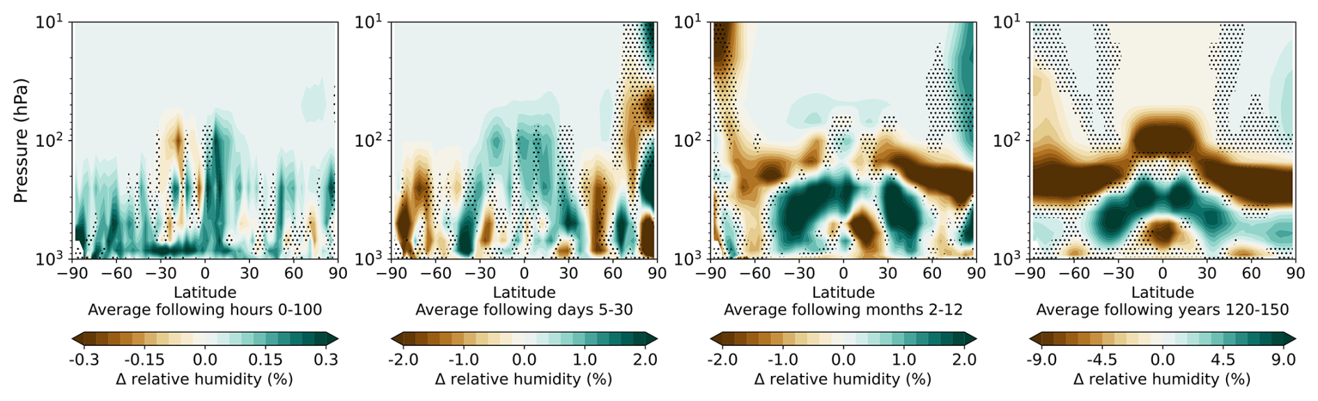
Figure 8 shows the vertical distribution of zonal mean relative humidity anomaly. While specific humidity reacts to the cooling air temperature by decreasing in the whole atmosphere, especially strong in the tropics and over all timescales (not shown), relative humidity displays a pattern of increase and decrease. During the first 100 h, relative humidity increases, apart from southern tropical latitudes that show a decrease. During the first month, an overall increasing pattern remains in the tropics, while higher latitudes show decrease. During the first year, the high troposphere dries, while the middle tropospheric layers experience a moistening. The lower troposphere shows a regular pattern of moistening and drying, and only at $\pm {\mathrm{65}}^{\circ }$ does the whole troposphere dry. The pattern further intensifies on long-term timescales.

Figure 8 Same as Fig. 7 but for atmospheric relative humidity anomaly in %.

To further analyse the short-term adjustments of relative humidity, it makes sense to differentiate between trends on land and over sea, since they react very differently to the forcing on short timescales due to their different heat capacities. Hence, Fig. 9 shows the zonal means of relative humidity change for the first two timescales averaged over ocean (Fig. 9a) and land (Fig. 9b) only. To investigate the effects of changing vertical atmospherical stability Fig. 9 also shows the same for change of vertical velocity (Δwap) (averaged over ocean (c) and land (d)). As wap is defined positive downwards, red colours of Δwap indicate an increase in downward movement or a decrease in upward movement and vice versa for blue colours.

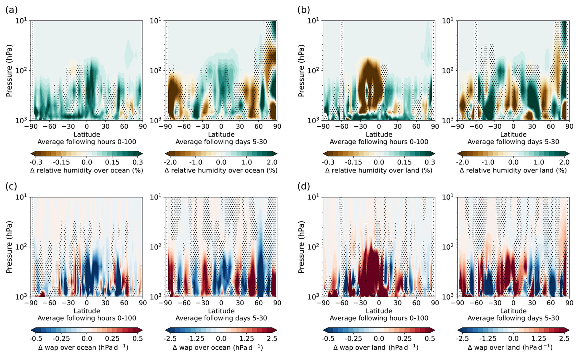
Figure 9 Zonal mean of relative humidity anomaly (in %) for the first 100 h and days 5–30 (corresponds to the first two timescales of Fig. 8) averaged over ocean (a) and land (b) only and the same plots for vertical velocity (wap, positive downwards) anomaly in hPa d⁻¹ averaged over ocean (c) and land (d).

Over the ocean, the lower troposphere cools down quicker than the sea surface on timescales of hours to days. This leads to a decrease in vertical stability, which then increases convective activity, especially over tropical oceans (see Fig. 9c). Increased convection dries the boundary layer, thereby reducing near-surface specific humidity. In order to compensate for the deficit in humidity, evaporation and thereby latent heat flux increase, which then results in an increase in surface relative humidity (see Fig. 9a) and precipitation in tropic latitudes.

Over land, vertical stability very much depends on location, albedo and heat capacity of the respective surface type. There is a strong reduction in convection over the tropics due to the reduced radiative forcing (see Fig. 9d) and resulting reduction in sensible heat flux, especially over the Sahara. This leads to trapping of moisture in the boundary layer and an increase in relative humidity in near-surface layers (see Fig. 9b). Latent heat flux is reduced in equatorial regions, and overall less moisture is transported into the higher troposphere, which reduces relative humidity in the free troposphere (see Fig. 9b).

The significant differences between land and ocean surface response are strongest during the first hours after the onset of forcing, but they are still clearly visible during the first month and lead to changes in land–sea circulation and moisture transport.

Cao et al. (2012) described similar effects, although of opposite sign in response to a +4 % increase in the solar constant experiment. After 5 d they found a decrease in relative humidity in the boundary layer of 1 % over land and an increase of around 0.1 % over ocean. This is a similar magnitude compared to our findings; however, with our approach we also found an increase in near-surface relative humidity in response to a negative solar forcing, as the drying of the boundary layer due to reduced stability is compensated for by increased latent heat flux.

For the vertically resolved atmospheric cloud fraction, the four models only provided monthly data. Hence for the zonal mean of the atmospheric cloud fraction anomaly, shown in Fig. 10, no data were available for the first timescale and the first monthly mean was plotted as the “first 31 d” timescale. This is not fully identical to other plots of this kind because, if available, the daily data from day 5–30 were averaged, not including the first 4 d, while in the case of the atmospheric cloud fraction, the average of the whole month is plotted.

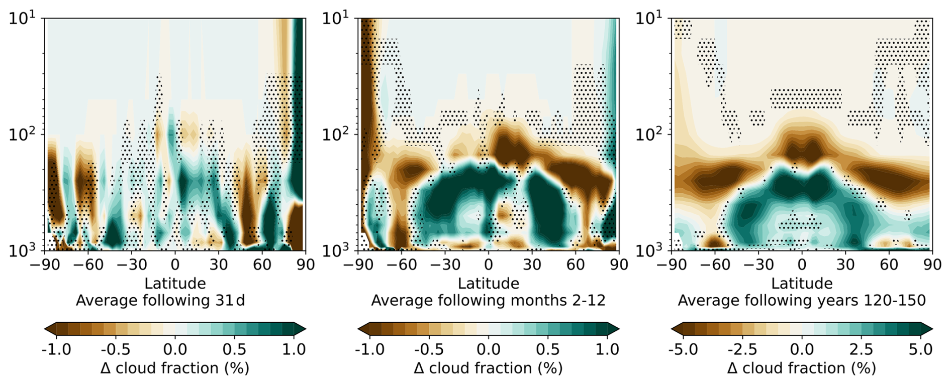
Figure 10 Same as Fig. 7 but for atmospheric cloud fraction anomaly (in %) on 49 pressure levels (the three other models were interpolated to CanESM5 levels). Only monthly data were provided. Hence, the first timescale (hours 0–100) is missing.

As expected, the atmospheric cloud fraction anomaly pattern in Fig. 10 is overall very similar to the pattern of relative humidity in Fig. 8.

During the first month, the atmospheric cloud fraction increases in the tropics over ocean, while it decreases over land. However, the increase over the ocean dominates the zonal mean. Higher latitudes show a pattern of decreasing and increasing cloud fraction, where circulation strength changes (also visible in the vertical velocity anomaly in Fig. 9).

Over the first year, tropical regions experience the strongest negative radiative forcing, leading to less absorption of shortwave radiation in the troposphere and reduced convective heating from the lower troposphere. Because the colder air contains less water vapour, also the greenhouse effect is reduced, a positive feedback. This way, condensation levels are reached at lower altitude, and high clouds shift downwards. This leads to a decrease in cloud cover at 150 hPa and an increase in cloud cover around 250 hPa, mirroring the same effects in relative humidity. An exception of the overall increasing cloud fraction in the troposphere is just above ±60°, where the subtropical jet stream strength is reduced, due to reduced temperature contrast between mid-latitudes and high latitudes, and weaker storm systems produce less dynamic lifting, reducing cloud formation in those regions.

On longer timescales, the overall pattern further intensifies, as do atmospheric temperature and relative humidity patterns.

A distinct drying pattern in the relative humidity at the lower troposphere in the tropics (see Fig. 8) is not visible in the atmospheric cloud fraction because it appears at a height of generally low cloud cover.

4 Discussion

The aim of this study was to understand and analyse atmospheric processes that take place on timescales of hours, days and months after the onset of a negative solar forcing. We did so using the output of four different climate models that participated in the abrupt-solm4p experiment of CFMIP of CMIP6. These fully coupled simulations provide the opportunity to get a more realistic view on rapid adjustments in the climate system, as all components of the climate system are allowed to react to the forcing at the same time, instead of fixing (sea) surface temperatures. This allows for a more realistic interplay between the different components, although a −4 % solar constant forcing still needs to be considered a highly idealised forcing compared to, for example, transient climate change.

Our approach is based on the assumption that the short timescales of hours, days and months are dominated by rapid adjustments rather than by surface-temperature-mediated changes. We showed in Fig. 4 that for these three timescales, the simulated change in surface temperature cannot explain the simulated change in TOA fluxes. Only when adjusting it by the rapid adjustments found in the linear regression plots of Sect. 3.1 do temperature-mediated TOA flux change and simulated TOA flux change start to coincide after around 4 years in model mean. This corresponds to the time the linear regression plots show non-linearities and is likely connected to adjustments of system with high inertia, like cryosphere and vegetation, that happen on longer timescales or a delay in the response of the deeper ocean compared to the surface (SST pattern effect, e.g. Andrews et al. (2015)). Since our study concentrates on adjustments during the first year, these kinds of adjustments are not considered here.

Having the atmosphere, surface and deep ocean react to the forcing at the same time poses the challenge of a possible overlap of adjustments to the forcing and temperature-mediated processes. Nevertheless, our findings do agree in many points with findings of other studies that applied a variety of different methods, often more restrictive compared to our approach, which we discuss in the following.

Smith et al. (2018) analysed adjustments to five different forcing agents, among them a +2 % solar forcing, using 11 global climate models with fixed-SST in combination with radiative kernels. Similar to our results, they found that in the case of solar forcing, rapid adjustments reduce ERF. However, the adjustments we found using the linear regression method were overall stronger (∼ 35 % ± 5 % of IRF) in relation to the original forcing than they were in the case of Smith et al. (2018) (∼ 10 % ± 5 % of IRF). According to their findings, the changes in surface, tropospheric and stratospheric temperature adjustment contribute the most to counteracting the forcing. Our method does not allow a quantification of the different effects in the same way, but we also see a decrease in surface temperature as well as atmospheric temperature in global mean, which will reduce the TOA forcing. The atmospheric cooling leads to a reduction in the specific humidity in the whole atmosphere, which reduces the warming effect of water vapour in the atmosphere and is hence expected to increase TOA forcing, which is also shown in Smith et al. (2018). We find a very similar pattern of cloud fraction change to that reported by Smith et al. (2018), though of opposite sign, since this study was based on a reduction in the solar constant. We calculated the anomaly of cloud radiative effect in order to estimate the influence of cloud adjustments on the ERF. However, the cloud radiative effect anomaly contains masking effects, which hamper the comparability with studies that specifically quantified cloud adjustments. Nevertheless, when assuming that all initial signals in ΔCRE_TOA can be attributed to masking, rather than changes in cloud properties, this initial signal can be subtracted, leaving a more variable but positive cloud adjustment, like what was found by Smith et al. (2018).

Russotto and Ackerman (2018) conducted a study using G1 data from the geoengineering MIP (GeoMIP) of CMIP6, where a 4-fold CO₂ increase is balanced by a matching decrease in solar constant. The decrease is between −3.2 % and −5 %, thus of similar magnitude as was used in the abrupt-solm4p experiment. That experimental setup avoids a long-term change in surface temperature. Hence, all signals are a mix of adjustments to the two different forcing agents. They find a significant cooling of the higher troposphere, as was shown in our results and a warming of the polar regions, which we also detected. However, in their case it is probably linked to the so-called “residual polar amplification”, which can be seen in only CO₂ forcing experiments and is of higher magnitude and higher signal-to-noise ratio (SNR) than the signal found in this study. A significant difference in the atmospheric temperature change is the stratospheric cooling, which is much stronger in the results of Russotto and Ackerman (2018) due to adjustments to 4×CO₂ because of the increased LW radiation to space (Manabe and Wetherald, 1975). This effect is much stronger than the stratospheric cooling in response to solar forcing, which we see in our results. Although of similar magnitude, cloud fraction changes in the G1 experiment seem to be dominated by adjustments to CO₂, since Russotto and Ackerman (2018) find opposite signals to what we found. This is supported by the findings of Smith et al. (2018), who estimate cloud adjustments to CO₂ forcing to be twice as large as to a positive solar forcing with twice as strong IRF. However, Smith et al. (2018) quantified a positive solar forcing, and Aerenson et al. (2024) show that responses to positive and negative solar forcing can differ, not only in sign, but also in strength and pattern.

Furthermore, for their solp4p experiment Aerenson et al. (2024) find an increasing cloud cover over tropical land regions, decreasing cloud cover in higher latitudes over land and an overall reduction in cloud cover over ocean. We find similar patterns, though of opposite sign, as expected for a reduction in the solar constant. The same is true for the CRE components they calculated for a solp2p experiment. However, when applying their newly developed method, Aerenson et al. (2024) find an overall positive cloud radiative adjustment to a +4 % solar constant forcing, meaning that clouds further increase the initial solar forcing rather than reducing it, mostly via their shortwave effects due to changes in cloud fraction. This is the opposite effect compared to what was found by, for example, Smith et al. (2018) or Virgin and Fletcher (2022) and what our results indicate. Aerenson et al. (2024) show that there can be substantial differences in adjustments to positive and negative solar forcing and linearity cannot be assumed. Nevertheless, they also find the opposite sign to Smith et al. (2018), who also analysed positive solar forcing simulations. All studies report high uncertainty for cloud adjustments, and, similar to our study, Aerenson et al. (2024) only had data from four climate models they could base their analysis on. In their case, one model predicts negative cloud adjustments, and only two models show significantly positive adjustments. Moreover, their method combines fixed-SST with fully coupled model runs in order to quantify adjustments to solar forcing. Several studies have shown that the two approaches, although showing similar results, can also show deviations due to differences in, for example, dynamical adjustments of land–sea circulation. The approach of Aerenson et al. (2024) may mistakenly interpret CO₂ forcing offsets caused by the fixed-SST method as adjustments to solar forcing.

All in all, this disagreement shows how challenging a proper quantification of cloud adjustments is and that they remain a source of high uncertainty in climate models.

Salvi et al. (2021) conducted a study on adjustments, using idealised atmospheric heating experiments, which were then fitted to the diagnosed heating curve of different forcing agents. This way, they found that the vertical centre of mass, what they call the “characteristic altitude”, determines the cloud adjustments. Like Smith et al. (2018) and our study, they found negative cloud adjustments to, in their case, a +3 % solar forcing. In their observed and fitted data they found a decrease in relative humidity and cloud fraction at around 300 and 800 hPa, which corresponds well with the increased cloud fraction we find in these altitudes. There is some deviation in the upper troposphere–lower stratosphere (UTLS) region, where we find a significant reduction in cloud fraction and relative humidity, while Salvi et al. (2021) only diagnosed minor changes in cloud fraction and the fitted algorithm predicted a decrease. This again could either be an effect of different methods, as Salvi et al. (2021) themselves attribute the deviation to insufficient resolution of the vertically heating curves in these high altitudes. Nevertheless, some differences in response to positive and negative solar forcing can take place, as Aerenson et al. (2024) found, especially when considering non-linear processes like phase changes in clouds.

Moreover, our study supports the findings of other studies like Kamae et al. (2019) that adjustments can also depend on the season of initialisation. The strong response in Arctic surface temperatures, which we attribute to a disruption of the polar vortex, is an effect of initialising the forcing in January.

A challenge our study faced was the sparse dataset it is based on. Only four models participated in the solm4p experiment, each providing one run. A higher number of models and ensembles would increase the reliability of our findings. However, due to the strong nature of the forcing, and since every model initialised the experiment from a different point in their piControl runs, we do expect that the four models cover different climate variability modes. Hence, an agreement of several models on the sign of an adjustment effect and overall high model-mean anomalies indicate a signal that exceeds possible climate variability. For all analysed climate variables, the first month is the timescale with lowest agreement of the models on the sign of the signal. This is to be expected, since responses will strongly depend on the position of, for example, pressure systems at the moment of onset of forcing. For example, this becomes apparent in the Arctic surface temperature anomaly during the first month, where all models simulated strong changes in surface temperature. We attribute those to a disruption of the polar vortex, but the actual pattern differs between the models, since it will be influenced by the original state of the atmosphere. Nevertheless, Fig. 6 shows strong signals for several high-latitude regions, where at least three out of four models agree on the sign. Therefore, we interpret it as a rapid adjustment rather than a random signal due to climate variability and expect to find similar signals for more realistic forcing scenarios like volcanic eruptions.

One surprising aspect of this study was the disagreement of the long-term development of the models, especially when examining cloud related variables. While the models agree well on the TOA radiative budget anomaly, they differ in how the long- and shortwave components contribute to this and how the fluxes interact with changes in cloud properties. In a number of cloud variables and, hence, in the cloud radiative effect anomalies, high latitudes and tropics show an opposite response, and the global mean signal is determined by the dominating region, which differs between the models. Further investigation into the single models and parametrisation as well as possible tuning would be necessary to understand the different outputs. Though this was out of the scope of this study, it shows how even climate models of the newest generation still struggle to simulate short- and long-term change of cloud properties, and further research on the topic is necessary.

5 Conclusion

This study offers insights into the dynamics of short-term adjustments within the climate system in response to an instantaneous radiative forcing. This was done through the analysis of the abrupt-solm4p experiment of CMIP6. By simulating a 4 % reduction in the solar constant, the experiment provides a valuable framework for understanding how the Earth climate system reacts to changes in solar energy input, especially on shorter timescales of days to month.

Following the linear regression method developed by Gregory et al. (2004), we find rapid adjustments of 3.6 W m⁻² in response to an instantaneous negative solar forcing of $-\mathrm{10}\mathrm{W}{\mathrm{m}}^{-\mathrm{2}}$. Other studies like Smith et al. (2018) also found that RA counteracted an initial solar forcing but of smaller magnitude (∼ 10 %). However, the amount of reduction differs, based on the method and number of participating models.

For this study, data from fully coupled climate models were used, leading to a possible overlap of adjustment and feedback mechanisms. However, it was shown that surface temperature change cannot explain the variability of the TOA radiative budget over the course of the first hours, days and months. Instead, the cloud radiative effect anomaly was found to closely match the TOA budget variability, indicating cloud property changes to be a major contribution to overall atmospheric adjustments. However, the method applied in this study did not allow for a quantification of cloud adjustments at TOA. Instead, global distribution patterns of a number of climate variables were analysed in order to find characteristic patterns (fingerprints) of atmospheric adjustments that could help explain the underlying mechanisms.

The analysis reveals significant alterations in various climate variables, including surface and atmospheric temperatures, relative humidity and vertical velocity, as well as a number of cloud properties. All models simulate decreasing atmospheric and surface temperatures, beginning immediately after the onset of forcing in January. One exception was an increase in Arctic surface temperature, which we attribute to a weakened polar night jet and thereby disruption of the polar vortex, leading to warm-air intrusions. Significant differences were found between the response of relative humidity over land and over ocean. Over ocean, decreased vertical stability, due to a quicker cooling of the lower troposphere compared to the ocean surface, leads to increased convection and thereby drying of the boundary layer, which is then compensated for by an increased latent heat flux, leading to an increase in relative humidity and mid-level cloud cover. Over land in the tropics, convection is reduced and moisture effectively trapped in the boundary layer, which leads to an increase in relative humidity in near-surface layers and a decrease in relative humidity and cloud cover in the higher troposphere. This highlights the complex interactions and differences between the land and sea response. On timescales of months, overall lower temperatures lead to drying of the troposphere, and the decrease in solar energy in the tropics leads to a reduction in ascent, less convection and a descending high cloud layer.

While other experiments of CMIP6 are designed in a way that influence of seasonal and climate variability are reduced using a number of different initialisation dates, the abrupt-solm4p simulations use only one date (1 January). This could be viewed as a limitation of this study. Nevertheless, if the scientific community strives for a validation of new discoveries about rapid adjustments in climate models with e.g. satellite measurements, more realistic simulations are crucial in order to further improve state of the art climate models. This study showed that the positioning of the forcing can have significant influence on the resulting short-term adjustments, in this case, the disruption of the polar vortex and consequently warming of the higher northern latitudes.

Moreover, the described adjustments to a reduced solar constant may resemble adjustments to more realistic forcing scenarios. After large volcanic eruptions a global stratospheric aerosol scattering layer can form a few months after the eruption. This aerosol layer reduces the amount of shortwave radiation that reaches the surface, which could lead to similar adjustment effects as simulated for a reduced solar constant. However, in the case of the abrupt-solm4p experiment, the forcing is instantaneous and constant, which makes it easier to differentiate between instantaneous forcing, short-term adjustments and long-term feedbacks. Therefore, it is a useful tool on the way to a more in depth understanding of realistic forcing agents of more transient nature. By elucidating the short-term adjustments that occur in response to reduced solar radiation, essential insights can be provided that can inform risk assessments associated with solar radiation management methods. Understanding these adjustments is vital for anticipating potential local impacts, such as droughts or floods, which can have significant consequences for communities and ecosystems.

In conclusion, this study identifies several characteristic adjustment processes as well as a number of challenges related to the current approaches in quantifying adjustments. By integrating short-term adjustment processes into climate modelling efforts, the scientific community can improve the accuracy of long-term climate predictions and develop more effective strategies for addressing the challenges posed by climate change.

Appendix A: Linear regression plots for components of TOA radiative budget

Analogous to the total TOA radiative budget, the yearly mean of the components of the TOA budget anomaly, i.e. downward shortwave flux change $\mathrm{\Delta }{\mathrm{sw}}_{\mathrm{all}\mathrm{sky}}^{\downarrow }$, upward shortwave flux change $\mathrm{\Delta }{\mathrm{sw}}_{\mathrm{all}\mathrm{sky}}^{\uparrow }$ and upward longwave flux $\mathrm{\Delta }{\mathrm{lw}}_{\mathrm{all}\mathrm{sky}}^{\uparrow }$, was also plotted against the surface temperature change, and linear regressions were applied in Figs. A1b, A1c and A1d. For comparison, Fig. A1a shows the linear regression for the TOA radiative budget anomaly (same as Fig. 1). Offsets after 1 month of simulation were marked as red crosses to provide insight into the contribution to overall RA of the single radiative components. The multi-model-mean intercepts of the linear regression with the radiative flux axis are shown in the respective figures as well as in Table 2 of the main paper. As determined by the experiment conditions, Δsw^↓ (Fig. A1b) is held constant over the whole experiment time. However, a seasonal variation occurs due the elliptical orbit of the Earth and produces a small offset between the first-month value (January) and the yearly mean values.

In contrast, Δsw^↑ (Fig. A1c) exhibits a clear approximately linear relation to ΔT. All models simulate an instantaneous response of Δsw^↑ in reaction to the reduction of solar constant (red cross), depending on the planetary albedo.

Figure A1d shows the same linear regression for upward longwave radiation anomaly (Δlw^↑). All models simulate a clear linear relationship between Δlw^↑ and ΔT with an intercept of around $-\mathrm{1}\mathrm{W}{\mathrm{m}}^{-\mathrm{2}}$, which equals the longwave adjustment as no instantaneous adjustments are expected.

The linear regression method was also applied to the cloud radiative effect anomaly ΔCRE_TOA and its short- and longwave components (ΔCRE_TOA,sw and ΔCRE_TOA,lw). The results are shown in Fig. A2. Analogous to the TOA radiative flux, components' contributions to ERF and RA were calculated and are provided in Table 2 in the main paper.

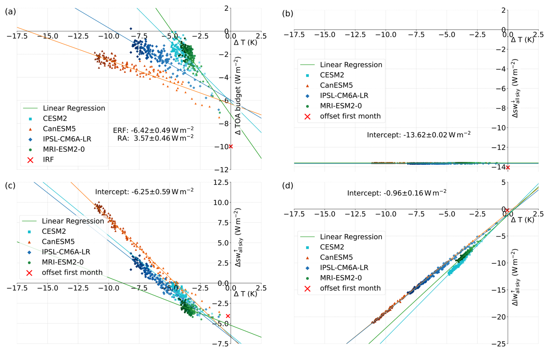
Figure A1 Linear regression plots for yearly global mean TOA radiative flux anomalies in W m⁻² vs. change in yearly global mean surface temperature (ΔT). Plotted are the anomalies of (a) the TOA radiative budget, (b) the downward shortwave flux at TOA, (c) the upward shortwave flux at TOA and (d) the upward longwave flux at TOA. The respective initial offsets after 1 month are marked as a red cross. Deepening colours indicate temporal development.

Figure A2 Same as Fig. A1 but for linear regression plots for yearly global mean ΔCRE_TOA (a) and its long- and shortwave components ΔCRE_TOA,sw (b) and ΔCRE_TOA,lw (c).

Appendix B: Geographical distribution of TOA radiative fluxes on different timescales

B1 Geographical distributions of Δ TOA budget and its components

Figure B1a, b and c show the geographical distributions of the TOA radiative flux anomalies shown in Fig. 2 of the main paper. Since only MRI-ESM2-0 provided daily data, the first timescale does not display a multi-model mean but only the data of the MRI-ESM2-0 model. For the following 30 d, the January mean of all four models was averaged.

Figure B1a clearly shows the uneven distribution of downward shortwave flux anomaly due to the chosen starting point of the experiment on 1 January. As the region of maximum sun exposure moves further north during the following month, the averages over the first year and the following 120–150 years then show the expected symmetric distribution after a full seasonal cycle with the strongest forcing in the tropics.

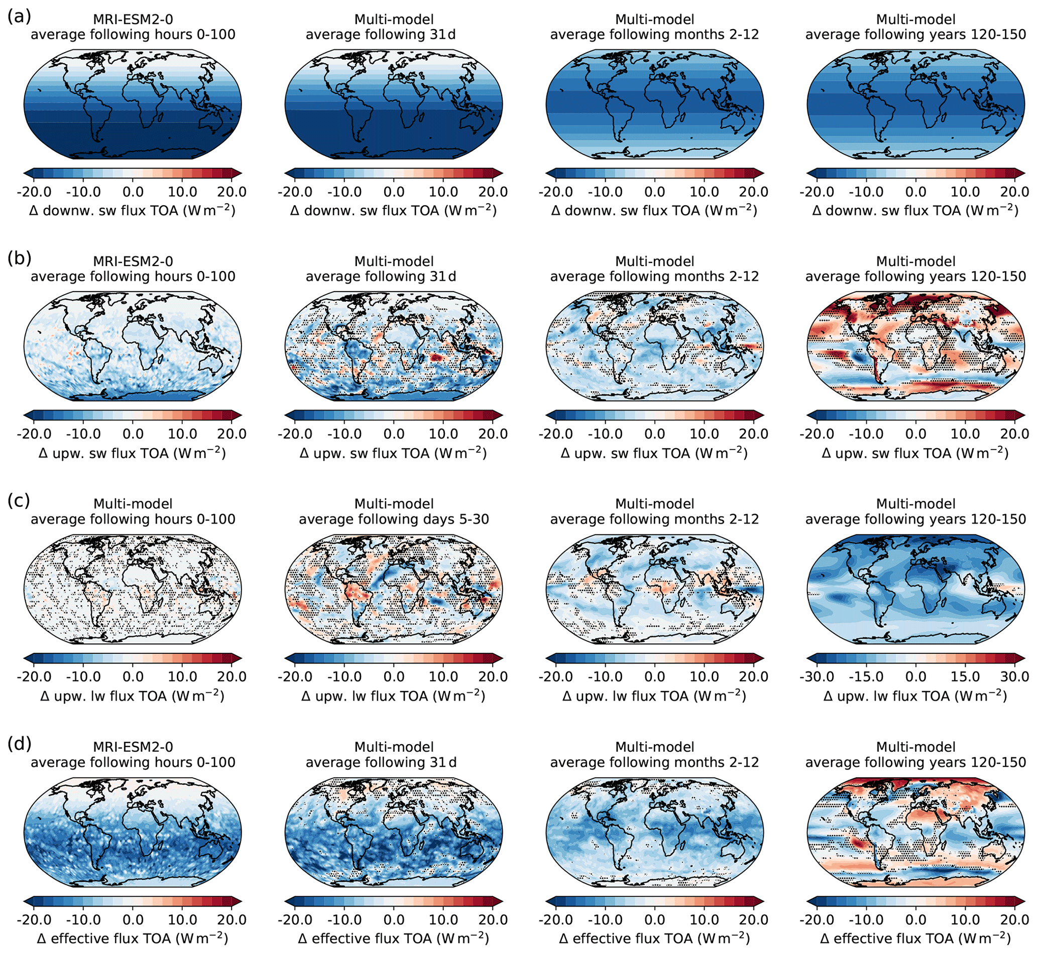
Figure B1 Multi-model-mean global distribution of TOA radiative fluxes in W m⁻² averaged over four different timescales after the onset of forcing (100 h, 31 d, months 2–12, years 120–150). Plotted are (a) the downward shortwave radiative flux anomaly at TOA, (b) the upward shortwave radiative flux anomaly at TOA, (c) the upward longwave radiative flux anomaly at TOA and (d) the radiative budget anomaly at TOA. For the first timescale of (a), (b) and (d) only data from MRI-ESM2-0 are plotted because other models only provided monthly data. Regions where fewer than three out of four models agree on a sign of anomaly are dotted.

The upward shortwave flux in Fig. B1b reflects the distribution of the initial forcing but locally adapted according to surface or cloud albedo. Especially Antarctica and the region of the westerlies with usually high cloud cover show the strongest reduction in upward shortwave flux. Similar to several other aforementioned climate variables, the uncertainty is high for the following 30 d. Only the reduction of upward shortwave flux in Antarctica remains relatively constant during the first month, due to the unchanged snow albedo. In contrast to that, South America shows an increased reduction in upward shortwave flux compared to the surrounding regions and the first timescale. Since surface albedo remains relatively constant over the first month, this effect can be attributed to changes in cloud properties in reaction to an overall drying and reduced ascent over tropical land areas. Hence, cloud liquid and ice water paths are decreased over South America, coinciding with an overall decrease in specific humidity and total cloud fraction. This leads to less scattering of downward shortwave flux and, hence, more absorption by the surface. Because of its comparably low albedo (mostly green vegetation), the upward shortwave flux is reduced, and, hence, the planetary albedo is decreased. The opposite effect can be seen in the Indian Ocean, where liquid and ice water paths as well as total cloud fraction are increased, thereby increasing planetary albedo. During the first year, the overall negative trend of upward shortwave flux continues, with only local positive anomalies, where surface albedo or cloud properties are changed. On longer timescales, the cooling of the surface leads to sea ice spreading further to lower latitudes, which strongly increases surface albedo in the respective areas, leading to positive anomalies in upward shortwave flux. Similar surface albedo effects are visible on land, where snow cover is increased, especially in mountain areas. In contrast to that, increased upward shortwave flux over ocean is linked to an increase in cloud fraction, liquid and ice water path. Depending on whether the increase due to increased surface albedo or cloud cover, or the overall decrease due to the reduction of incoming shortwave radiation is stronger, the sign of the global mean upward shortwave flux anomalies differs between different models.

Figure B1c shows the anomaly of upward longwave radiative flux. Overall, decreasing atmospheric and surface temperatures lead to a decrease in outgoing longwave radiation with time. However, this effect is partly compensated for by the reduction in water vapour. This process is especially effective in the tropics, where colder temperatures lead to a reduced amount of water vapour. This reduces the water vapour greenhouse effect and thereby optical depth of the atmosphere, which then in turn can result in a more effective radiative cooling. This can lead to slightly positive signals in outgoing longwave radiation over tropical land areas. Cloud property changes further amplify these effects. During the first two time steps, anomalies are small, and the uncertainty is high. The few stronger signals coincide with the upward shortwave signals described before due to cloud property changes. The longwave effects often partially counteract the shortwave effects because an increase in cloud liquid and ice water path will lead to more reflection of shortwave radiation, but at the same time, more upward longwave flux is absorbed, thereby decreasing TOA upward longwave flux. Over the first year, upward longwave radiation further decreases due to the reduction of surface temperature, the so-called Planck effect. It becomes the dominant effect on longer timescales, clearly showing the effect of Arctic Amplification as a stronger cooling in Arctic latitudes. The only exception is an increase in upward longwave radiation northeast of Oceania, where cloud liquid and ice water path are reduced significantly, counteracting surface cooling effects.

Figure B1d displays the global distribution of the radiative budget anomaly at TOA. During the first 100 h, the reduced downward shortwave flux is the dominating influence on the TOA radiative budget anomaly, and the distribution of the shortwave forcing is clearly visible. Short-term adjustments reduce the overall loss of energy at TOA only locally, e.g. where precipitation is increased in the tropics, which coincides with changes in cloud properties. During the first month, the pattern remains relatively unchanged. Only the strong changes in surface temperature in high northern latitudes, due to the aforementioned disruption of the polar vortex, lead to a reduction in upward longwave radiation lost to space. Since the region is not directly influenced by the reduced solar constant, this longwave effect leads to a slight increase in the radiative budget anomaly at TOA in high northern latitudes.

Over the first year, the TOA radiative budget anomaly is still dominated by the reduced solar constant. Local effects due to changes in cloud properties do not have significant effects on the radiative budget anomaly at TOA because shortwave and longwave effects compensate for each other.

On longer timescales, the TOA radiative budget anomaly reaches a new balance, and the global mean anomaly approaches zero. However, the global distribution of TOA radiative budget anomaly shows a significant pattern over different latitudes, depending on the strength of local short- and longwave effects. The Planck effect generally acts against the radiative shortwave forcing by reducing the upward longwave radiation. Hence, the TOA radiative budget anomaly is positive, where either the reduction in upward longwave radiation is stronger than the forcing or the upward shortwave flux anomaly is also negative, counteracting the initial forcing.

B2 Geographical distributions of ΔCRE_TOA and its components

Figure B2 shows the global distribution of the total ΔCRE_TOA (Fig. B2c), as well as its shortwave and longwave components, ΔCRE_TOA,sw and ΔCRE_TOA,lw (Fig. B2a and b).

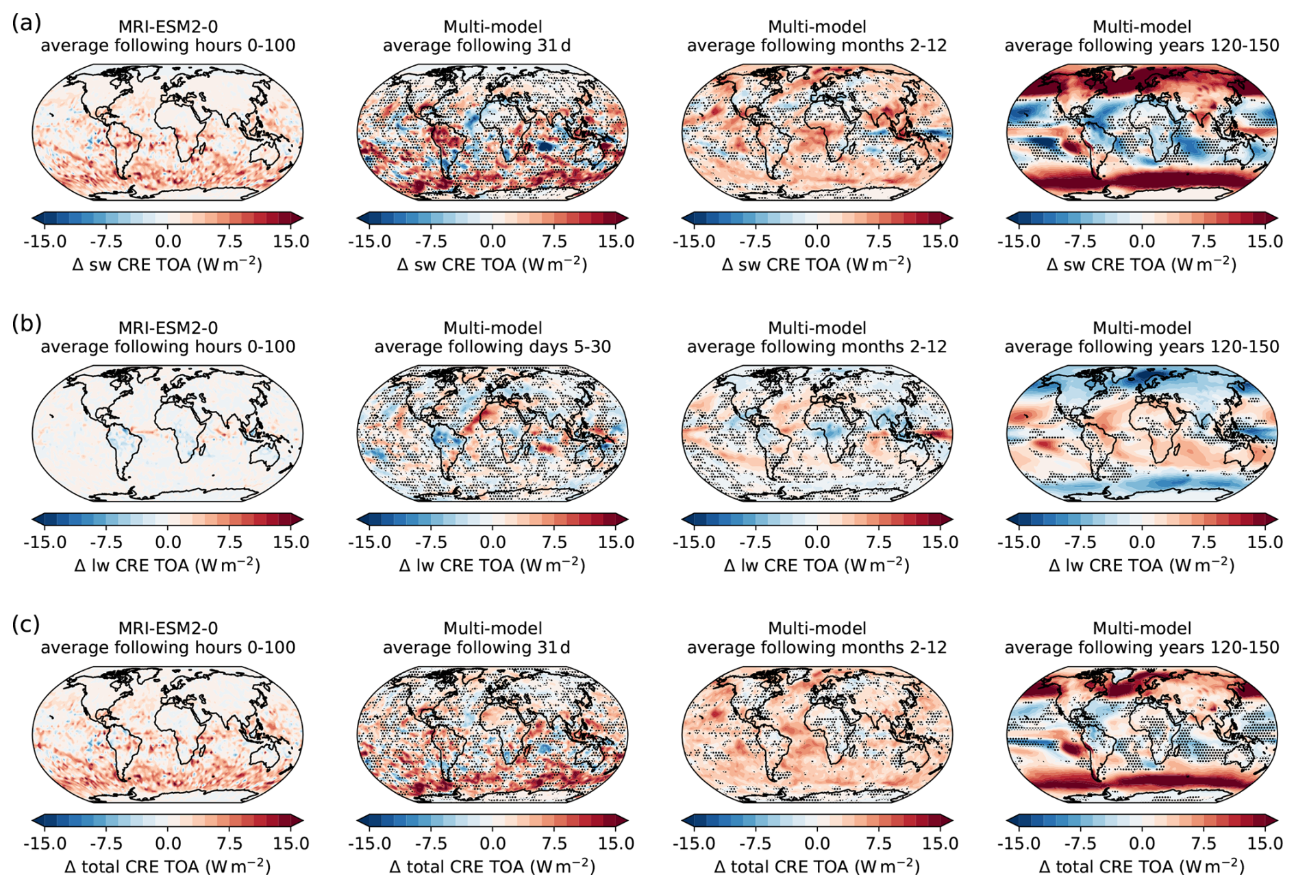
Figure B2 Same as Fig. B1 but for (a) shortwave and (b) longwave effects and (c) the total TOA cloud radiative effect anomaly (ΔCRE_TOA,sw, ΔCRE_TOA,lw and ΔCRE_TOA) in W m⁻².

During the first 100 h, ΔCRE_TOA,sw is strongest in the Southern Hemisphere, where the shortwave forcing is strong and cloud cover is high. Hence, the increased ΔCRE_TOA,sw is mostly an effect of cloud masking, rather than being caused by changes in cloud properties. The only exception is Antarctica, where the high snow albedo suppresses any possible shortwave cloud radiative effects. In contrast to that, ΔCRE_TOA,lw remains relatively unchanged, and only in the tropics do some stronger signals appear, roughly coinciding with areas of increased precipitation, indicating increased condensation and bigger droplets that absorb more longwave radiation and lead to a positive ΔCRE_TOA,lw. Vice versa, areas of decreased total cloud fraction over central Africa, Peru and northern Australia lead to negative ΔCRE_TOA,lw.

During the first month, ΔCRE_TOA,sw further strengthens, and the decrease in cloud liquid and ice water path over South America mentioned before, as well as the opposite effect in the Indian Ocean, is visible as areas of increased and decreased ΔCRE_TOA,sw, respectively. The same regions show up in the ΔCRE_TOA,lw as regions of stronger signal but of opposite sign due to the aforementioned compensation of short- and longwave effects. Moreover, a region of increased cloud ice water path and cloud fraction on the west coast of Africa produces a clear signal of decreasing ΔCRE_TOA,sw and increasing ΔCRE_TOA,lw, since less shortwave radiation is scattered, and more longwave radiation is transmitted to space.

Over the first year ΔCRE_TOA,sw remains positive overall, with a more homogeneous distribution over the globe, due to the more homogeneous distribution of the forcing after a complete seasonal cycle. Only Oceania shows a distinct decrease in ΔCRE_TOA,sw and increase in ΔCRE_TOA,lw, where all cloud properties analysed in this study show a distinct reduction. However, as described before, short- and longwave effects compensate for each other in a way that the changes in cloud properties, mentioned above, are not visible in the total ΔCRE_TOA.

On long-term timescales, ΔCRE_TOA,sw shows a clear correlation with increased surface albedo at high latitudes, leading to a strong positive masking effect. Moreover, a decreased cloud liquid water path, e.g. over high latitudes and the equatorial Pacific, leads to an increase in ΔCRE_TOA,sw in these regions, while an increasing cloud liquid water path over tropical oceans has the opposite effect. In contrast to that, ΔCRE_TOA,lw shows stronger correlation with the cloud ice water path anomaly, since ice clouds have a generally stronger longwave effect than liquid clouds. In total, shortwave effects are overall stronger and, thus, dominate ΔCRE_TOA, while longwave effects only appear at certain locations of strong longwave anomalies. Hence, a separate consideration of short- and longwave effects can help to understand the underlying processes better, compared to only considering the total ΔCRE_TOA. Nevertheless, masking effects impede a clear detection of cloud adjustments based on the cloud radiative effect.