Contribution of gravity waves to shear in the extratropical lowermost stratosphere: insights from idealized baroclinic life cycle experiments

Mixing significantly influences the redistribution of trace species in the lower stratosphere, potentially being the dominant factor in forming the extratropical transition layer (ExTL). However, the role of small-scale processes contributing to mixing is poorly characterized. In the extratropics, mixing processes are often linked to stratosphere–troposphere exchange (STE), which occurs frequently during baroclinic life cycles, e.g., near tropopause folds, cut-off lows, or stratospheric streamers. Gravity waves (GWs), a dynamical feature of these life cycles, can potentially contribute to STE and mixing in the lower stratosphere. We present a series of baroclinic life cycle experiments with the ICOsahedral Non-hydrostatic (ICON) model to study the impact of GWs on the occurrence of vertical wind shear and consequent potential turbulence, an indicator for mixing in the lowermost stratosphere (LMS). Dry adiabatic simulations with varying spatial resolution reveal that the spatiotemporal occurrence of GWs depends on the model grid spacing and is closely linked to shear and turbulence generation. Further process understanding is gained from experiments incorporating physical processes like latent heating, (vertical) turbulence, and cloud microphysics. Introducing moist processes amplifies GW activity and turbulence potential, mainly driven by latent heat release and stronger baroclinic wave evolution with vigorous vertical motions. Turbulence parameterization has a lesser effect on the overall evolution without moisture, whereas it dampens the effect of latent heat release in moist simulations. Altogether, GWs substantially enhance vertical shear and potential turbulence occurrence in the LMS and thus can play a significant role in tracer mixing and, consequently, in the ExTL formation.

1 Introduction

Atmospheric gravity waves (GWs) play a pivotal role in the dynamics of the Earth's middle atmosphere, transporting energy and momentum and hence significantly contributing to the atmospheric energy budget. GWs are mainly generated in the lower atmosphere due to various sources such as topography, jet imbalances, fronts, convection, and strong wind shear (Fritts and Alexander, 2003; Achatz et al., 2024, and references therein). Jet imbalances here refer to regions within jet streams where deviations from geostrophic balance often result in strong vertical wind shear. These GWs propagate both vertically and horizontally, with a major portion of their momentum flux carried by GWs originating in the troposphere. During ascent, the amplitude of these GWs increases due to decreasing atmospheric density. In turn, this amplification can lead to saturation and thus breaking of the GWs. In this process, GWs deposit momentum, which in turn acts as a forcing mechanism for the large-scale circulation in the stratosphere and mesosphere (Andrews et al., 1987). Locally, GW breaking can cause turbulence in the stratosphere and mesosphere (Hodges, 1967).

In recent years, there has been growing interest in understanding the contribution of small-scale dynamics, specifically GWs, to stratosphere–troposphere exchange and mixing in the upper troposphere and lower stratosphere (UTLS) (e.g., Luderer et al., 2007; Kunkel et al., 2019; Lachnitt et al., 2023). The UTLS is an intriguing region for GW studies, serving as both source and sink, due to its characteristics of jet streams, strong inhomogeneities in wind fields, horizontal temperature gradients, and abrupt changes in atmospheric stability. While horizontal temperature gradients influence the background wind structure and baroclinicity, vertical stability affects wave amplification and dissipation. These characteristics chiefly influence GW propagation and are a potential source for GW dissipation. Regions of baroclinic instability and jet streaks are often associated with enhanced GW activity, forming hotspots where GWs are frequently generated and interact with the background flow (Plougonven and Snyder, 2005; Zhang et al., 2015a). Consequently, the UTLS serves as an important source region for GWs, shaping their propagation and interaction with larger-scale atmospheric processes.

GWs strongly influence the dynamical and thermodynamical structure of the atmosphere, particularly in the UTLS. By interacting with the background flow, GWs can amplify the strong vertical wind shear, from now on referred to as the vertical shear, often leading to regions of reduced static stability. Such interactions can give rise to the tropopause shear layer (TSL, Kaluza et al., 2021), defined as the occurrence frequency of enhanced vertical wind shear, where vertical shear is given by $S^{\mathrm{2}}={\left(\frac{\partial u}{\partial z}\right)}^{\mathrm{2}}+{\left(\frac{\partial v}{\partial z}\right)}^{\mathrm{2}}$, i.e., the squared vertical gradient of the horizontal wind components u and v. Following Kaluza et al. (2021), regions of enhanced shear are defined as those where S² exceeds a threshold value $S_{\mathrm{t}}^{\mathrm{2}}$, which corresponds to the 95th percentile of total S² values within a climatological dataset, that is to say, the region near the extratropical tropopause that is characterized by a maximum occurrence frequency of S² ≥ $S_{\mathrm{t}}^{\mathrm{2}}$. This statistical approach allows the identification of particularly strong shear events associated with tropopause disturbances. Observational studies suggest that GW-induced enhancements of shear can reach values on the order of 10⁻²–10⁻³ s⁻¹ (e.g., Lane et al., 2004; Kaluza et al., 2021), particularly in dynamically active regions such as baroclinic instability, jet streaks, and upper-level frontal zones (Koch et al., 2005; Wang and Zhang, 2007). These are also regions where clear air turbulence (CAT) frequently occurs, sometimes triggered by GW breaking or momentum deposition in strong background shear (Lane et al., 2004). Moreover, GWs play a pivotal role in modulating the stability of the tropopause inversion layer (TIL), a thin layer above the tropopause characterized by a sharp increase in static stability (Kunkel et al., 2014). Through wave breaking, momentum deposition, and induced instabilities, GWs can affect the vertical structure of stability and contribute to the sharp stratification of the TIL (Zhang et al., 2015b; Kunkel et al., 2019; Zhang et al., 2019). This bidirectional interaction between GWs and stability gradients is fundamental in maintaining the TIL structure, which acts as a barrier to vertical mixing and influences stratosphere–troposphere exchange (STE) (Erler and Wirth, 2011; Zhang et al., 2015b). However, the exact magnitude and representation of these processes remain sensitive to model resolution and the treatment of subgrid-scale GW processes, particularly in parameterized frameworks. This continues to be an area of active research and debate in both modeling (e.g., Plougonven and Zhang, 2014; Stephan et al., 2019) and observational (e.g., Geller et al., 2013; Jewtoukoff et al., 2015) studies.

GWs further significantly influence tracer transport and mixing in the UTLS and may also lead to the generation of turbulence. One way is to enhance the strong vertical shear, which leads to dynamical instabilities such as Kelvin–Helmholtz instability (KHI); another possibility is GW breaking at critical levels where the phase speed of these waves matches the background wind (e.g., Shapiro, 1978; Whiteway et al., 2004; Lane and Sharman, 2006), leading to localized turbulent mixing. These processes are prominent in the extratropical transition layer (ExTL), a chemical-tracer-based transition zone around the tropopause, where turbulence facilitates tracer exchanges and cross-isentropic mixing (e.g., Hoor et al., 2004; Pan et al., 2006). This mixing layer, where the tracer-based tropopause indicates a blurred boundary between stratospheric and tropospheric air masses (Hegglin et al., 2009), is a direct consequence of STE and turbulent diffusion. Moreover, the ExTL is part of the lowermost stratosphere (LMS), which can broadly be defined as the region between the height of the extratropical and tropical tropopause (Weyland et al., 2025). The LMS corresponds to the so-called “middle world”, where isentropic surfaces intersect the tropopause, allowing for quasi-isentropic exchange between the tropical troposphere and extratropical stratosphere (Holton et al., 1995). The upper boundary of this layer is commonly approximated by the 380 K isentrope, representing the height of the tropical tropopause (e.g., Appenzeller et al., 1996; Olsen et al., 2013; Wang and Fu, 2021). The LMS encompasses the ExTL, which is characterized by changes in chemical tracer gradients and has been supported by trajectory-based studies (e.g., Hoor et al., 2004; Berthet et al., 2007; Hoor et al., 2010).

Observational studies including airborne measurements and radiosonde data show that turbulence in the ExTL enhances the vertical redistribution of chemical tracers, such as ozone and water vapor, as well as other radiatively active species, impacting UTLS composition and influencing radiative and dynamical processes (Hoor et al., 2004; Birner et al., 2002; Birner, 2006; Zhang et al., 2015a). This and the modulation of potential vorticity (PV) gradients near the tropopause suggest that GWs might play a role in enhancing mixing and modifying the structure of the mixing layer (e.g., Kunkel et al., 2019). High-resolution numerical simulations emphasize the role of GWs in enhancing wind shear and triggering instabilities, leading to efficient mixing in the UTLS (e.g., Spreitzer et al., 2019). Additionally, simulations of mid-latitude cyclones reveal the impact of tropospheric jet streak, wind speed, shear enhancement, and GWs on CAT occurrence, highlighting their interaction with wind shear profiles (Trier et al., 2020; Lane et al., 2004). Evidence from the DEEPWAVE (Deep Propagating Gravity Wave Experiment) campaign has shown that orographic GWs can induce cross-isentropic mixing through turbulence (Lachnitt et al., 2023). This mixing led to irreversible changes in tracer distributions, providing direct proof of the role of GW-induced turbulence in shaping the UTLS composition. These findings underscore the coupling between GW dynamics and mixing processes, particularly within the ExTL, where chemical gradients are sharpest and small-scale dynamics play a crucial role in vertical transport and mixing, further influencing large-scale atmospheric processes.

Sources of GWs in the extratropical atmosphere can be manifold. Many GWs result from flow over topography (e.g., Durran, 1995; Lachnitt et al., 2023), while GWs can also emerge above convective systems (e.g., Lane et al., 2001; Fritts and Alexander, 2003; Lane and Sharman, 2006; Alexander et al., 2010). Another important source is baroclinic waves with their jet and fronts (O'sullivan and Dunkerton, 1995; Plougonven and Zhang, 2014). In the extratropical atmosphere, this source is commonly associated with baroclinic waves but still can be regarded as a less well understood source of GWs. Surface fronts and upper-level jet streams associated with baroclinic wave development generate GWs primarily through spontaneous imbalance, where deviations from geostrophic flow trigger GW emission (Plougonven and Zhang, 2014; Zhang et al., 2015b). Particularly, these GWs that are emitted along jet streaks and frontal zones propagate more horizontally and, while interacting with the background flow, can foster the generation of shear and turbulence (e.g., Plougonven and Snyder, 2005; Zülicke and Peters, 2006; Trier et al., 2020; Kaluza et al., 2021). This source of GWs is particularly significant because baroclinic life cycles, which are quasi-periodic, being large-scale wave patterns in mid-latitudes, are a persistent feature of extratropical atmosphere, with four to eight distinct baroclinic waves typically evident (Hoskins et al., 1985). Ultimately, the GWs associated with baroclinic waves affect the tropopause structure and may significantly contribute to mixing in the UTLS. In particular, their contribution for shear occurrence in the UTLS has not been systematically studied despite the indications presented in recent years (e.g., Kunkel et al., 2014; Zhang et al., 2019; Kaluza et al., 2021).

A way to approach baroclinic life cycles and the processes within is to use an idealized numerical representation of these waves. In fact, several studies have used idealized setups to study GWs within baroclinic life cycles. In a series of experiments, O'sullivan and Dunkerton (1995) were the first to show that GWs, more precisely inertia GWs, emerge in dry adiabatic baroclinic life cycles in regions of the jet stream. However, they did not analyze their role for shear or turbulence generation. Wei and Zhang (2014) studied the effect of additional moisture in the setup on the appearance of the GWs. Although they showed that the convectively generated GWs emerge much earlier in fast-growing moist baroclinic waves, their role in the subsequent mixing was not explored. Kunkel et al. (2014) showed that GW from baroclinic waves can alter the tropopause structure and generate an environment prone to mixing and STE. However, they did not systematically study the role of GWs on shear generation and the consequences for turbulence occurrence.

In this study, we utilize some ideas from previous studies to better understand the role of GWs associated with baroclinic life cycles in the generation of shear and consequent turbulence in the LMS. We do this in the framework of idealized baroclinic life cycle experiments of varying complexity with the ICOsahedral Non-hydrostatic (ICON) model. Specifically, we address the following questions: (i) how does the ICON model resolve GWs in idealized baroclinic life cycle simulations, and where do these GWs emerge relative to the tropopause location? (ii) Are these GWs associated with instabilities in the lowermost stratosphere, which could lead to mixing? (iii) How much do GWs contribute to the enhanced shear in the lower stratosphere?

Idealized numerical experiments of baroclinic waves, and, in particular, the representation of GWs in such simulations, have certain limitations. While the appearance of GWs and their effect on shear are tightly coupled to the model resolution, the findings of this study might be regarded as a lower estimate of the effect of GWs on shear generation. Also note that this study specifically focuses on GWs generated by jet–front systems during baroclinic wave evolution. GWs from other sources, such as orography and convection, are not considered, as their adequate representation would require a different model configuration and substantially higher resolution, which are beyond the scope of this study. Nonetheless, our idealized setup allows a controlled investigation of the effect of GWs emitted within baroclinic disturbance while isolating their role from other processes.

The paper is organized in the following manner: in Sect. 2, we introduce the model configuration and give an overview of the experiments used in this study. In Sect. 3, we provide a detailed examination of the evolution of baroclinic life cycles and the spatial resolution sensitivity experiments, with the GWs appearing therein. Then, we take a closer look at some GW events. Section 4 discusses the occurrence of shear and turbulence in the LMS and their relation to the small-scale GWs in different baroclinic life cycles. We further provide a comprehensive analysis of the possible contribution of GWs in the generation of TSL in Sect. 5. Finally, we summarize outcomes from the idealistic approach and provide some concluding remarks in Sect. 6.

2 Model configuration and numerical experiments

2.1 Adiabatic model configuration

We conducted baroclinic life cycle (BLC) experiments in an idealized configuration of the non-hydrostatic ICON model (Zängl et al., 2015). Firstly, the dynamical core of ICON is used to simulate the dry adiabatic experiments. In this study, the ICON model is set up over the global domain, from the surface up to a height of 35 km. ICON uses the icosahedral triangular grid that provides nearly homogeneous coverage of the globe, alleviating numerical stability concerns associated with traditional latitude–longitude grids. To mitigate the reflection of upward-propagating GWs back into the computational domain, the sponge covers the upper 13 km of the model domain. Free slip boundary conditions are applied at the surface in ICON, assuming zero normal wind velocity, representing smooth flow over the surface without friction. The ICON model effectively simulates atmospheric dynamics by numerically solving the fully compressible, non-hydrostatic Navier–Stokes equations. The time integration of ICON combines the Matsuno scheme and the Heun scheme (also known as the trapezoidal scheme), commonly known as the predictor-corrector scheme (Zängl et al., 2015). Numerical hyper-diffusion is used to reduce the impact of inherently produced grid-scale checkerboard error patterns on numerical simulations. In the dry dynamical experiments, we exclude the topography and moisture, which eliminates the possibility of the generation of GWs by topography or diabatic heating. Thus, the GWs in this simulations are generated internally.

2.2 Physical parameterizations

The atmospheric physics module of ICON comprises a multitude of schemes designed to depict diabatic and turbulent processes at the subgrid scale and their influence on the resolved circulation. In our simulations, we want to investigate the impact of certain physical processes on GWs. In particular, our focus is to examine the impact of latent heating and turbulence on the GWs and, ultimately, the emergence of shear and dynamic instability in the LMS. To accomplish this, we include a minimal set of physical parameterizations that reliably represent these processes. A detailed description of the formulation for such diabatic processes is given in Prill et al. (2020). We briefly outline the schemes used in our simulations, with further details provided in the next section.

2.2.1 Turbulence: vertical transfer and diffusion

We employ the moist turbulence scheme TURBDIFF (TURBulent DIFFusion) developed by Raschendorfer (2001), which emphasizes the distinction between turbulence and potential non-turbulent components of the subgrid-scale energy spectrum. This distinction introduces additional scale interaction terms in the prognostic turbulent kinetic energy (TKE) equation, accounting for extra shear production of TKE driven by non-turbulent subgrid-scale flow structures. This scheme can also amplify the intensity of turbulent vertical mixing. Turbulent effects in the horizontal direction are neglected, which is a valid approximation for simulations on the mesoscale, meaning that horizontal homogeneity is assumed. Therefore, the Boussinesq approximation is taken into account while parameterizing only vertical turbulent fluxes. Furthermore, the vertical change in specific humidity q_v and cloud water q_c, as well as the vertical shear of the horizontal wind components, has a substantial impact on the TKE budget equation. In the case of moist simulations, TURBDIFF includes processes related to saturation adjustment, which leads to latent heating and impacts the overall energy budget. Further information is provided in Raschendorfer (2001).

2.2.2 Cloud microphysics and latent heat release

In ICON, cloud microphysics parameterization uses a closed set of equations to calculate the formation and evolution of condensed water in the atmosphere. These provide the latent heating rates for the dynamics. Latent heating can occur as part of the microphysics scheme, chiefly via the saturation adjustment and the convection scheme, which leads to convective precipitation. The saturation adjustment process converts any supersaturation into cloud water or ice, releasing latent heat and thus influencing atmospheric stability. Notably, the employment of saturation adjustment leads to latent heating, which impacts the overall energy budget. This excess energy significantly influences the dynamics of the atmosphere, marking a significant difference from the dry simulations, where such effects are absent. The present study uses a single-moment microphysics scheme (Seifert, 2008), which predicts specific humidity q_v along with the specific mass content of four hydrometeor categories: cloud water, rainwater, cloud ice, and snow. This study solely focuses on understanding the impact of microphysics and, specifically, the associated latent heat release of the large-scale clouds on GWs, excluding the convective scheme, which would necessitate a more intricate configuration, including radiation and surface fluxes.

2.3 Model experiments

2.3.1 Initial state

For our initial state, we follow the setup proposed in the Dynamical Core Model Intercomparison Project 2016 (DCMIP, Ullrich et al., 2017) test case. The initial state is composed of a zonally symmetric background state, which is in thermal wind balance, and a perturbation to trigger a faster baroclinic wave evolution. The background state is initiated globally, whereas the perturbation is introduced only in the Northern Hemispheric UTLS. Consequently, a baroclinic wave will only emerge in the Northern Hemisphere within a period of about 15 d. We will thus focus only on the atmospheric state of the Northern Hemisphere.

Figure 1 shows the initial background state for zonal wind, potential temperature, potential vorticity, and specific humidity. In DCMIP, a weak, Gaussian-shaped wind perturbation is introduced at the center of the model domain, which points to the location (20° E, 40° N) at the altitude of the tropopause. The mid-latitudinal jets at 45° N/S are centered slightly below the tropopause, with a horizontal mean surface temperature of T=288 K. Moreover, the zonal wind is derived under the thermal wind balance. A moist variant of the dry dynamical test is considered here to understand the impact of moisture feedback on the development of the baroclinic wave. The moisture field is initially available only for simulations including moisture.

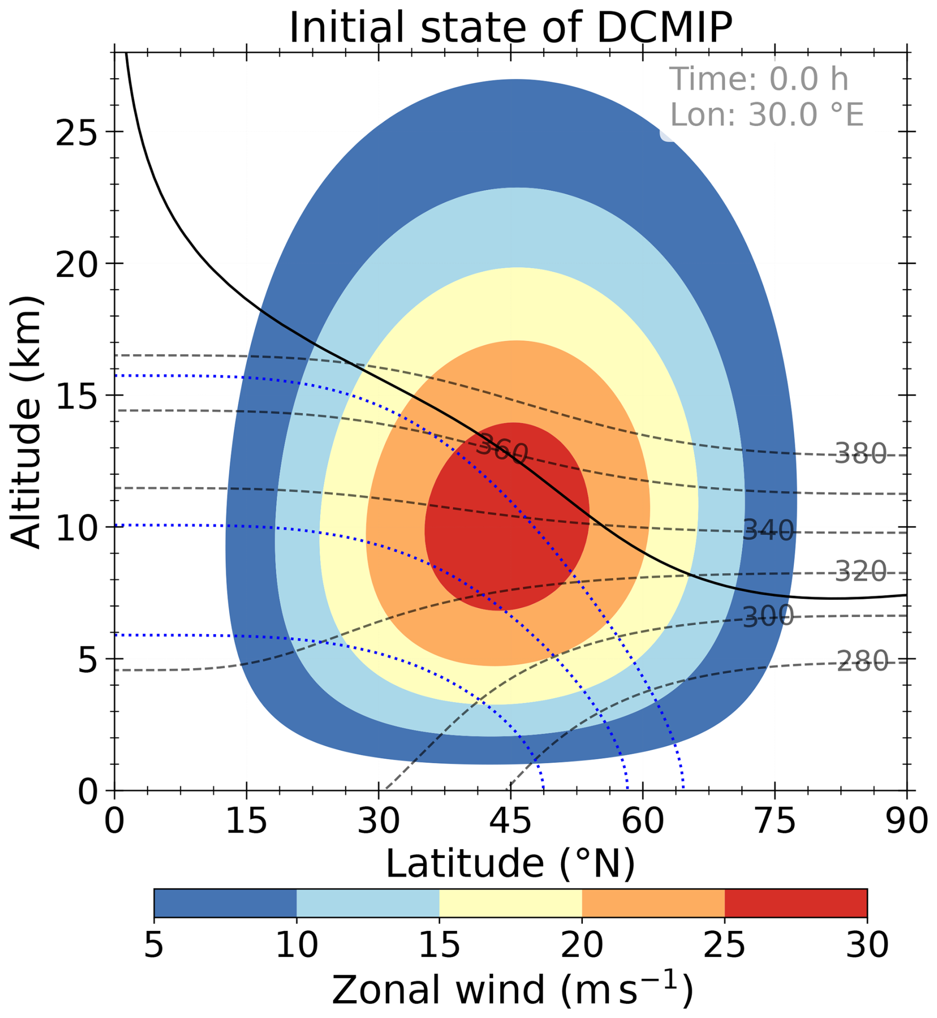
Figure 1 Zonally symmetric balanced initial conditions at 30° E longitude: zonal wind (shaded contours, 5 m s⁻¹ spacing), potential temperature (dashed gray lines, 20 K spacing, starting with 280 K in the lower-right corner), and specific humidity q_v for values 2, 0.2, and 0.02 g kg⁻¹ (dotted blue lines, from bottom to top). The black thick line marks the location of the dynamical tropopause, defined as the 3.5 PVU potential vorticity isosurface.

The DCMIP case with the zonal wind perturbation leads to a life cycle resembling a case known as life cycle type 1 (LC1; Thorncroft et al., 1993). This type shows the development of a stratospheric streamer along with anticyclonic wave breaking. A second case uses a perturbation of the stream function. As such, not only the zonal wind but also the meridional wind is directly perturbed (see Ullrich et al., 2014, for details). We abbreviate this case as DCMIP stream and note that this case has some resemblance to the life cycle type 2 described in Thorncroft et al. (1993). We will discuss both cases in our result sections because the two solutions provide some coverage of the life cycles observed in the real atmosphere.

2.3.2 Dry and moist baroclinic life cycle experiments

In total, we will discuss the results from 20 different BLC experiments (see Table 1). The life cycles vary in their initial state, the model resolution, or through the addition of physical processes. We conducted 10 simulations with a dry adiabatic setup, five each for the two initial states wind and stream (see Table 1). Our focus is primarily on the dry adiabatic simulations, with additional physics intended to provide a first basic insight into the effects of the respective physical processes. In these simulations, we varied the underlying horizontal grid from 13 km (R03B07 in ICON grid nomenclature) to 80 km (R02B05). We changed the number of vertical levels between 40 and 100 while keeping the domain height constant at 35 km in altitude. These levels resulted in roughly 900 or 300 m grid spacing in the UTLS. The simulations with 20 km horizontal grid spacing and 100 vertical levels will be regarded as our reference simulation (REF), for which we also conducted the majority of the physics-added simulations. The other simulations are either denoted as high (HRES), medium (MRES), or low (LRES) simulations. This setup strategy allows us to study the emergence of GWs, shear, and potential turbulent regions in our simulations.

Table 1 Summary of idealized DCMIP experiments performed using ICON.

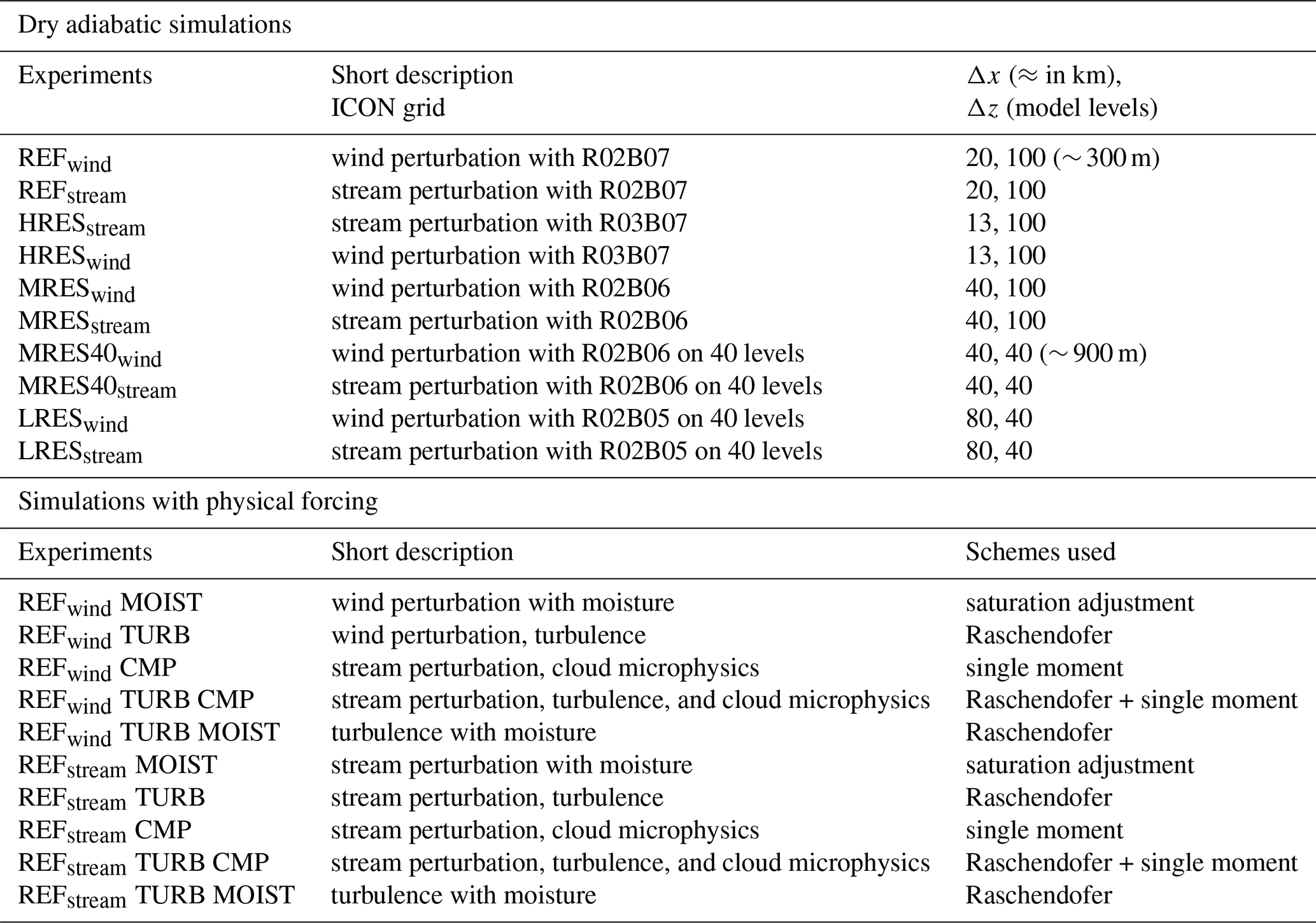
^∗ MOIST: only saturation adjustment, CMP: saturation adjustment + bulk microphysics scheme.

In the next step, we perform sensitivity experiments focusing on non-conservative processes, including either turbulence (further denoted as TURB) or cloud microphysics (CMP). For both initial states, we study the effect of moisture and, particularly, the effect of latent heat release on the GW, shear, and turbulence appearance. Two simulations use only the saturation adjustment scheme of the model to mainly study this latent heat feedback (MOIST). Additionally, we run two more simulations with a simple cloud microphysics scheme to address potential additional effects (CMP). We note here that the MOIST simulations have been carried out for all resolutions used in the dry adiabatic setup. However, because the general difference between dry and moist simulations is consistent, independent of the resolution, only the results for the REF cases are shown and discussed further.

We also want to determine whether the turbulence parameterization affects the appearance of GWs, shear, and turbulence in our simulations. For this, we run two REF simulations with the turbulence parameterization turned on (TURB). Finally, we run four REF simulations with combinations of wind, stream, TURB, MOIST, and CMP to address the combined effects of these parameterizations and initial states. More details about the simulations are given in Table 1.

3 The DCMIP baroclinic life cycle and the occurrence of gravity waves

3.1 Baroclinic evolution and gravity wave appearance in the reference simulations

We start this section with a brief introduction of the main features of the baroclinic life cycle. First, we show the evolution of the baroclinic wave using isentropic potential vorticity for the two reference simulations. We then discuss the occurrence of GWs that emerge during the various stages of life cycles.

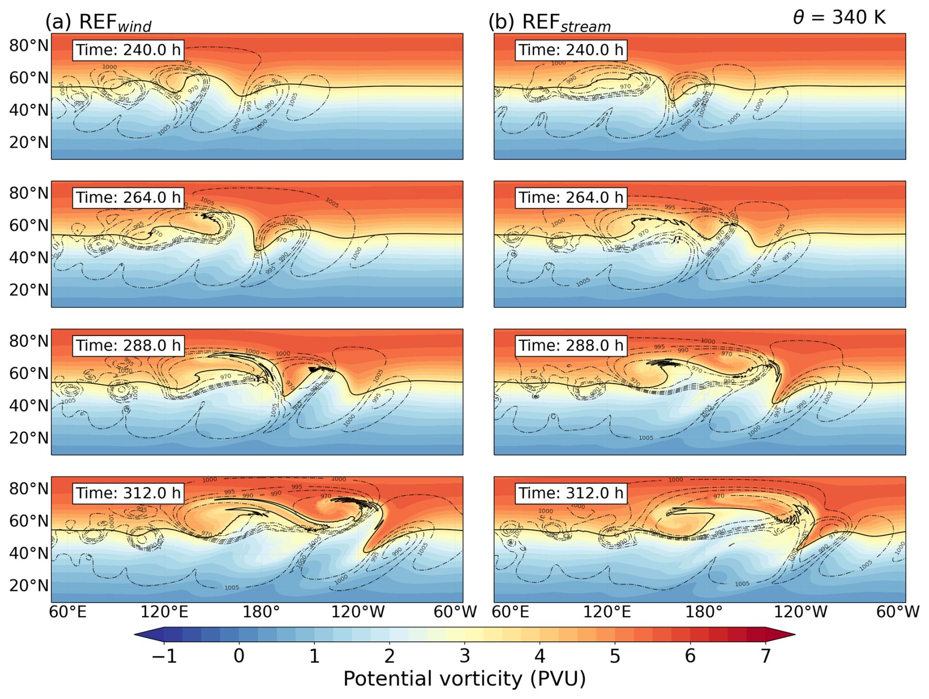
Figure 2 The evolution of the baroclinic life cycle for the (a) REF_wind and (b) REF_stream simulations. Horizontal cross sections of potential vorticity at 340 K isentropic surface and surface pressure (dashed contours) over the Northern Hemisphere after 240, 264, 288, and 312 h of model integration. The solid black line represents the 3.5 PVU, regarded as a dynamical tropopause.

Figure 2 provides an overview of the synoptic evolution of the baroclinic wave for two dry adiabatic reference simulations between 240 and 312 h after the simulation start. As will be shown later, this is the time period most interesting for our GW, shear, and turbulence analysis. The REF_wind and REF_stream simulations feature the same general characteristics of the life cycle as described in Ullrich et al. (2014) and cover the initial growth and rapid development of the baroclinic disturbance. The extratropical dynamical tropopause is defined in our simulations as the 3.5 PVU isoline (1 PVU = $\mathrm{1}\times {\mathrm{10}}^{-\mathrm{6}}$ K m² kg⁻¹ s⁻¹), following a commonly used definition in the literature (e.g., Hoerling et al., 1991; Erler and Wirth, 2011), and is highlighted by the black line in Fig. 2. Our life cycle evolves rather slowly, with the first signs of a substantially growing wave after 192 h. We consider this beneficial for two reasons: first, we can regard our results more conservatively because a slow evolution correlates with less GW emission; second, we think that numerical, spurious features occur less with a slower evolution.

As the time series highlights, both REF_wind and REF_stream baroclinic waves grow to substantial amplitudes, showing tropospheric and stratospheric intrusions, a PV streamer, and secondary cyclogenesis. PV streamers are identified as the high PV trough downstream of the anticyclonic wave breaking. Differences are observed in the size of the PV streamer and the strength of the tropospheric and stratospheric intrusions. Both life cycles exhibit baroclinic wave breaking. Despite their dry adiabatic nature, there are signs of PV non-conservation in the region of the steep PV gradients, potentially associated with numerical diffusion.

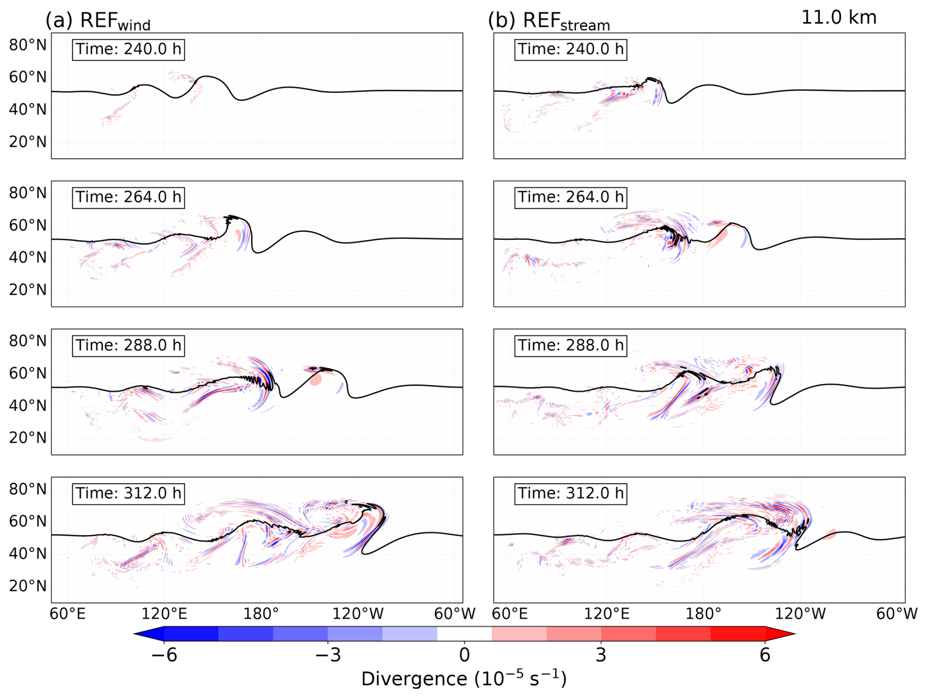
Figure 3 The evolution of the GWs for the (a) REF_wind and (b) REF_stream simulations. Horizontal cross sections of horizontal divergence at 11 km in altitude over the Northern Hemisphere after 240, 264, 288, and 312 h of model integration time, respectively. The solid black line represents the dynamical tropopause.

Figure 3 shows the divergence of the horizontal wind components and illustrates regions where GWs are present in two dry adiabatic reference simulations at various time steps at an altitude of 11 km. This altitude is close to the altitude of the jet stream core (see Fig. 1), thus representing well the situation of the tropopause region along the LMS and taken as a representative height for further discussion. As evident in Fig. 3, alternating signals in the horizontal divergence mark the presence of GWs in both reference simulations from 240 h onward. Wave activity was not prominent before the indicated simulation time (i.e., 240 h), but horizontal divergence fields highlight the emergence and subsequent intensification of wave-induced features thereafter. The GWs have their source of imbalances in the synoptic flow and propagate into the UTLS during life cycles. The wavelength of this wave mode can be deduced from the peaks in the divergent field. In many cases, the horizontal wavelength is on the order of a hundred kilometers, which is similar to wavelengths of inertia gravity waves.

A prominent sign of a GW emerges first after 240 h in the REF_wind simulation around 140° E. At 264 h, this feature is evident on the tropospheric side of the jet in the ridge around 170° E. Interestingly, the GW crosses the tropopause into the LMS (after 288 h) and spreads out in the stratosphere over the course of the next 24 h. The GW signatures are typically observed in the jet exit region and over the northwards reaching ridges of the baroclinic wave, especially in regions characterized by pronounced PV gradients with larger amplitudes (Plougonven and Snyder, 2005, 2007; Plougonven and Zhang, 2014). The jet stream in the UTLS partially excites the waves, indicating that both the surface front and the upper tropospheric jet–front system contribute as sources of these small-scale waves. This indicates that the background flow significantly influences the wave characteristics during their propagation. The larger spectrum of GWs was observed after 312 h when the baroclinic wave undergoes breaking. The GW characteristics adhere to the phases of baroclinic wave development. This aligns well with the fact that the growth rate of flow imbalance correlates with the growth rate of baroclinic waves, which, in turn, strongly correlates with the frequency of GWs.

The REF_stream experiment (Fig. 3b) reveals comparable temporal evolution of GWs but with slight variations in the location of GW development. The prominent signatures and the curl-up feature were noticed 1 d prior to REF_wind, resulting in the earlier appearance of GW modes. Three strong GW packets appear after 288 h, moving poleward and towards the west. The remarkable feature here is that the wave modes develop clockwise, representing the clockwise evolution of baroclinic waves. After 312 h, the REF_stream BLC undergoes cyclonic breaking in the LMS. Overall, this cyclonic wave breaking of baroclinic instability with stream perturbation resembles an LC2-type life cycle (Thorncroft et al., 1993). Even though the baroclinic wave in this form evolves quite swiftly, the wave breaking occurs later than in REF_wind. During the intensifying stage of BLC, features like substantial stratospheric intrusion and tropospheric wrap-up, along with the PV streamers in the horizontal divergence field, hint towards the potential turbulence in the lower stratosphere and could lead to STE.

3.2 Gravity wave occurrence: impact of horizontal and vertical grid spacing

In this section, we aim to answer how GWs emerge in low- and high-resolution simulations and how the occurrence, location, and properties of GWs are influenced by the horizontal and vertical grid spacing in the UTLS.

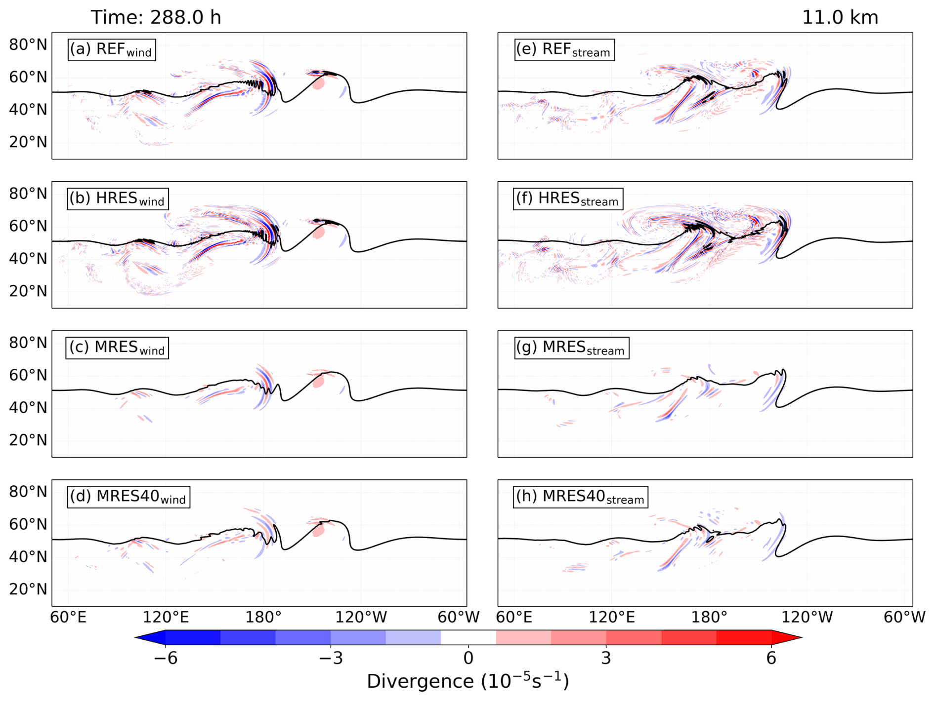
Figure 4 Evolution of GWs for simulations with varying grid spacings. Panels (a)–(d) represent simulations with wind perturbations for experiments REF, HRES, MRES, and MRES40, respectively, whereas panels (e)–(f) show simulations with stream perturbations for the same configurations. The figure displays the distribution of the horizontal divergence field at 11 km in altitude over the Northern Hemisphere after 288 h of model integration.

In the first step, we aim to assess the resolution dependence for which we use all of our dry adiabatic simulations with differing spatial resolutions. In general, the evolution of the baroclinic wave is similar across all dry simulations. While the large-scale structure remains consistent, mesoscale differences and slight variations in the exact location of the trough are evident. These are general features observed across all simulations, independent of the perturbation function. As a result, GW activity tends to emerge in similar regions among all dry simulations. Figure 4 illustrates the distribution of horizontal divergence at 11 km in altitude after 288 h for the respective simulations, highlighting these similarities. In the wind perturbation simulations, this is the region of the baroclinic wave ridge (see around 180° E after 288 h at 11 km) and above the trailing surface cold front. Other hotspots for GWs are evident, particularly upstream of the jet core, where the baroclinic wave induces strong vertical motion, and downstream near the tropopause, where GWs propagate along the sharp PV gradient of the streamer. Similar regions can be identified in the simulations with the stream function perturbation.

Besides these similarities, there are notable differences that can, of course, be expected. We noticed minimal differences in GW representation when varying the vertical resolution between 40 and 100 levels, with 100 levels adequately capturing the GW spectrum and its key features. The higher the model resolution, the greater the extent to which the GW spectrum is resolved; compare, e.g., the horizontal divergence field between the REF, HRES, MRES, and LRES (not shown) simulations. An example of wind perturbation is the region north of the surface cold front with more GW signals in the high-resolution simulations, which is virtually absent at coarser resolution i.e., LRES_stream (Fig. S1 in the Supplement). Henceforth, we exclude the LRES simulations, as they did not exhibit significant indication of GWs. A second notable difference is the amplitude of the divergent signal, which is larger in the high-resolution cases, aligning with previous findings that high resolution better captures GW signals and their propagation (Zhang, 2004; Plougonven and Snyder, 2005). There is minor sensitivity of medium-scale waves to enhanced horizontal resolution, implying that they are being adequately resolved in the REF and HRES simulations. These results support earlier studies showing that increased resolution enhances the ability to capture fine-scale GW structure and dynamics, whereas medium scale remains relatively insensitive (Plougonven et al., 2003; Kunkel et al., 2016).

3.3 Gravity wave occurrence: impact of non-conservative processes

In this section, we explore the impact of physical processes on the evolution of the baroclinic waves and the occurrence of GWs. For this, we compare the reference simulations with simulations including (1) latent heat feedback, i.e., MOIST, (2) a parameterization for cloud microphysics, i.e., CMP, (3) a parameterization for turbulence, i.e., TURB, (4) a combination of the parameterizations for cloud microphysics and turbulence, i.e., TURB CMP, and (5) turbulence parameterization with moisture, i.e., TURB MOIST.

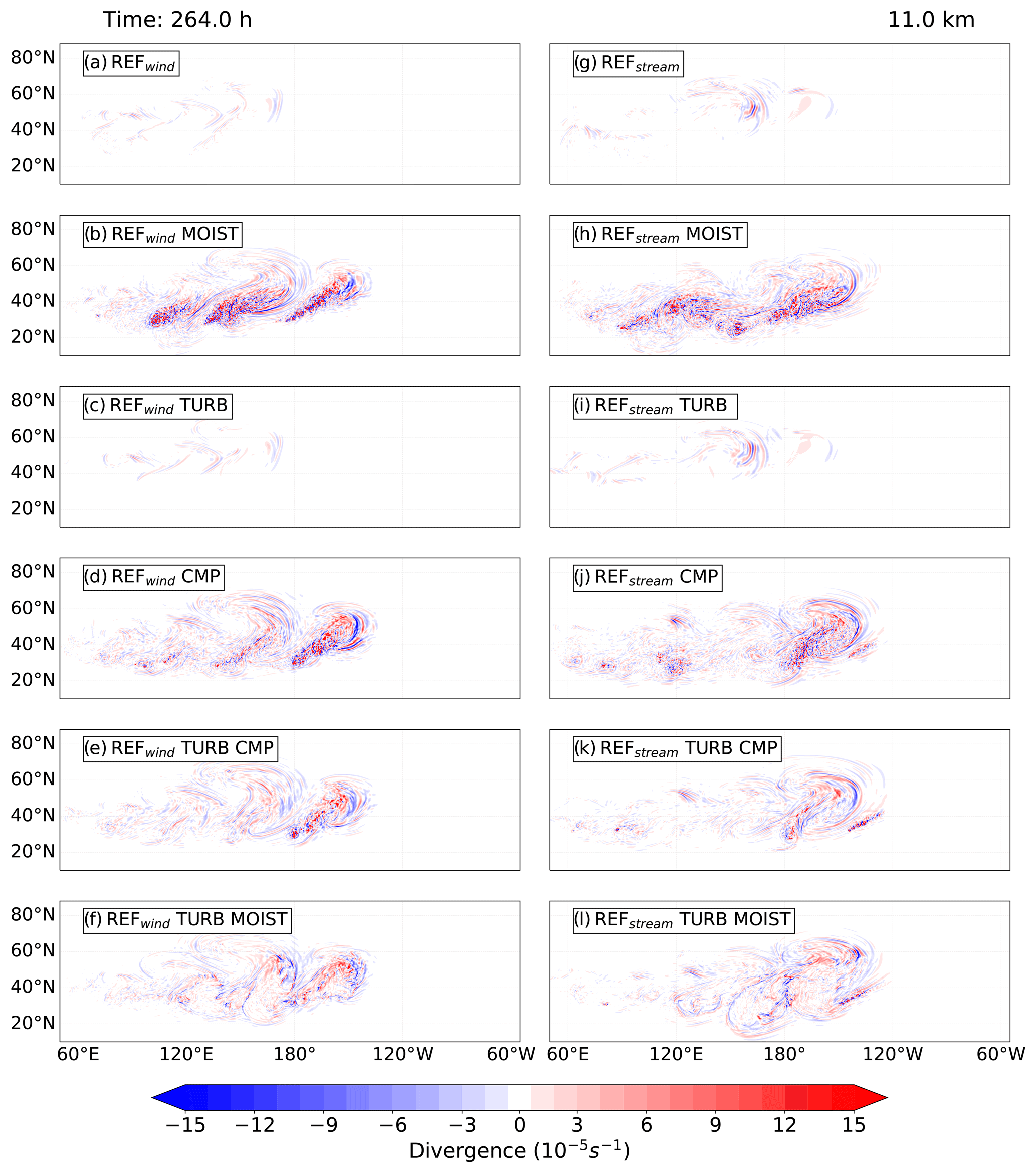
Figure 5 Same as in Fig. 4 but after 264 h for the simulations with varying physical processes. Top panels (a, g) represent the corresponding reference simulations.

The experiments investigate the influence of moisture on GW patterns within baroclinic waves, using both wind and stream perturbations. Figure 5 shows the 11 km horizontal divergence distribution at 264 h, highlighting the evolution of baroclinic waves and showcasing various GW modes during different stages of baroclinic wave development. Specifically, Fig. 5a captures the baroclinic structures in the REF_wind experiment, corresponding to the conditions in Fig. 5b for REF_stream. Moist cases (Fig. 5b, h) indicate noisy horizontal divergence, inconsistent with the patterns observed in the REF experiments. The MOIST simulation shows that baroclinic wave growth begins earlier than in the dry case, likely due to the release of latent heat being an additional energy source from moisture. Noticeable differences in the horizontal divergence pattern appear across the MOIST runs at this stage despite the initial moisture content being similar. The emergence of wave-like features before the appearance of the main GW pattern suggests spontaneous emission influenced by moisture. As a result, significant GWs are detected near large-scale structures. In conditions with moisture and saturation adjustment, the introduction of weak convective instability allows dry dynamic GW modes to prevail. Nonetheless, small-scale features indicative of GWs in the LS reveal consistent GW activity throughout the evolution of the moist baroclinic wave, which may warrant further analysis. Overall, the development of simulated moist baroclinic waves is qualitatively similar to the life cycles described by Wei and Zhang (2014) and Wei et al. (2016). However, isolating small-scale features from the large-scale dynamics in moist scenarios remains challenging, requiring additional steps to understand their impact on mixing.

We now move our discussion to assess the impact of bulk microphysics and turbulence parameterization on the development and characteristics of GWs. These experiments are conducted using the same spatial resolution as in the REF experiment. In the TURB simulations (Fig. 5c, i), the GW signature appears weaker, which could be due to the tendency of turbulence to reduce strong vertical gradients. Although turbulence acts against the effects of dry dynamics, the GW features observed in TURB are similar to the REF experiment. In the CMP experiment (Fig. 5d, j), similar horizontal divergence patterns as in the MOIST experiments are observed around 180° W/E, revealing that the latent heat release drives these patterns. The GW patterns in the LMS indicate that moisture inclusion leads to stronger updrafts, accelerating the evolution of the GW life cycle. Processes originating from lower tropospheric levels significantly influence GW activity, and similar effects are noted in experiments with saturation adjustment, i.e., MOIST, confirming that latent heat release, rather than microphysical processes, is responsible for the observed effect. Figure 5e, k and f, l display the TURB CMP and TURB MOIST cases, respectively, for both initial states. After 264 h of model integration, similar structures of GWs are observed in these experiments, with minor variations in GW characteristics. Specifically, GWs are more prominent in the TURB MOIST case, while the TURB CMP case shows differences in GW locations, with more subsequent GW modes emerging. The TURB CMP closely resembles the REF_wind CMP, suggesting that microphysical processes play a more dominant role than turbulence. Overall, distinct variations in GW patterns across all physics experiments are evident at this stage of the life cycle.

Taken together, in all MOIST physics experiments, latent heat release, a consequence of condensation, enhances vertical motions in the tropospheric region, which extend to the UTLS, creating sharp vertical gradients in stability and moisture. The air masses above are already undergoing a sinking motion, exhibiting enhanced upward motions. The processes in MOIST experiments differ fundamentally from those in dry scenarios, leading to significant variations in GW emergence in the lower stratosphere. The rapid, small-scale lifting processes associated with these upward motions drive the faster evolution of the GW life cycle, resulting in earlier wave breaking compared to the dry case. This demonstrates that incorporating moisture in the model accelerates GW evolution due to the enhanced upward motions caused by latent heat release throughout the life cycle. Nevertheless, the physical processes leading to GW occurrence seem to be similar in LC1 and LC2.

3.4 Gravity wave occurrence: connection with vertical shear

Our primary goal is to analyze the connection between GW occurrence in baroclinic life cycles and their potential to contribute to the formation of the shear layer above the tropopause and potential mixing. We have shown that GWs emerge under various initial states, grid resolutions, and process complexities. Before we dive deeper into the analysis of shear and turbulence in these simulations, we want to briefly highlight the spatial and temporal connection between the occurrence of GWs and enhanced small-scale vertical shear. For this, we again focus on the dry reference simulations.

The location of the GWs is analyzed via two metrics: the vertical wind perturbations w^′ and the absolute momentum flux. This is a momentum flux of the sub-synoptic scales, which we refer to as a first proxy for the momentum flux due to GWs (GWMF). We use w^′ instead of horizontal divergence because they are interconnected and w^′ is directly linked to the GWMF. As all the other prime quantities, w^′ here represents a filtered quantity. In order to quantify the GW perturbations from synoptic-scale structures, we use a hybrid approach that combines both a dynamical and a statistical approach to separate large- and small-scale components of the flow. To better focus on unbalanced GW dynamics, we first follow a dynamical approach in which we separate the wind components into divergent (e.g., u_div) and rotational components of the wind using the Helmholtz decomposition technique (Wei et al., 2022). We then apply a filter in spectral space to obtain only those contributions from a certain wavenumber onward. In this so-called statistical approach, we use a one-dimensional zonal FFT over the Northern Hemisphere and remove the contributions from wavenumbers 0 to 8, e.g., u^′ is defined as $u^{\prime }=u_{\mathrm{div}}-(u_{\mathrm{div}}{)}_{k\le k_{\mathrm{s}}}$, where k_s is the wavenumber cutoff, which splits the quantity into large-scale and small-scale components. In our idealized setup, sensitivity tests with k_s values of 12 or 20 showed no significant variation in the resulting GWMF or $S^{{\mathrm{2}}^{\prime }}$ distributions, indicating that our results are robust with respect to the choice of cutoff. Close to the poles, the filtering may remove GW signals as well, but we do not discuss GW contribution in those regions. We emphasize that our spectral definition of the background, along with the dynamical separation into balanced and unbalanced flow, is well justified in the lower stratosphere and consistent with prior studies (Stephan et al., 2019; Gupta et al., 2021; Wei et al., 2022), despite a different cutoff wavenumber used. The GWMF is then computed from the perturbation fields as follows:

$$\begin{array}{}\text{(1)}& \left|\mathrm{GWMF}\right|=\mathit{\rho }\sqrt{(\stackrel{\mathrm{‾}}{u^{\prime }{w}^{\prime }}{)}^{\mathrm{2}}+(\stackrel{\mathrm{‾}}{v^{\prime }{w}^{\prime }}{)}^{\mathrm{2}}},\end{array}$$

where ρ is the mean density and u^′, v^′, and w^′ are the zonal, meridional, and vertical velocity perturbations, respectively. The overline denotes a spatial average of the perturbation products (i.e., $\stackrel{\mathrm{‾}}{u^{\prime }{w}^{\prime }}$ and $\stackrel{\mathrm{‾}}{v^{\prime }{w}^{\prime }}$), computed using a low-pass filtering of the quadratic quantities that uses the same Gaussian spectral filter as mentioned in Kruse and Smith (2015). This averaging ensures that the flux estimates are physically meaningful, as direct pointwise computation of these second-order terms without low-pass filtering or areal averaging would not appropriately capture the wave-induced momentum transport (see also Wei et al., 2022). This approach is consistent with the statistical method of scale separation commonly used in GW studies (e.g., Lehmann et al., 2012; Wei et al., 2016). Additionally, the vertical shear for the small-scale components is estimated as:

$$\begin{array}{}\text{(2)}& S^{{\mathrm{2}}^{\prime }}={\left({\displaystyle \frac{\partial u^{\prime }}{\partial z}}\right)}^{\mathrm{2}}+{\left({\displaystyle \frac{\partial v^{\prime }}{\partial z}}\right)}^{\mathrm{2}}.\end{array}$$

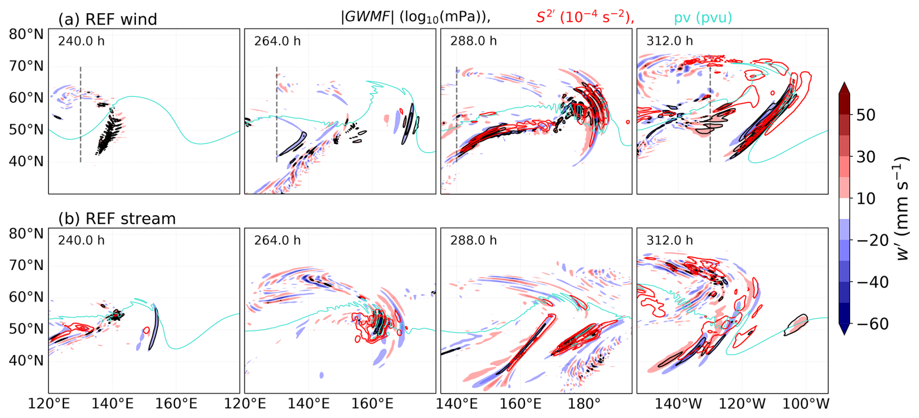
Figure 6 Horizontal evolution of 11 km perturbation vertical velocity w^′ in mm s⁻¹ from 240 h to 312 h of model integration for the REF_wind and REF_stream experiments. The absolute GW momentum flux (1.0, 1.5, and 2.0 in log10(mPa); black) and vertical wind shear perturbations $S^{{\mathrm{2}}^{\prime }}$ (1.0, 2.5, and 4.0 in 10⁻⁴ s⁻²; red) from the spectral domain are shown. The turquoise lines denote the 11 km dynamical tropopause where the potential vorticity equals 3.5 PVU.

Figure 6 shows the temporal evolution of GW packets reconstructed from the spectral domains at an altitude of 11 km for REF_wind and REF_stream. Velocity perturbations initially emerge above the low-level trough with small magnitudes, which then gradually intensify and form the organized GW structure in the eastern trough (see also Fig. 2, between 120° E and 100° W). These GW packets are identified by their horizontal wavelength (∼ 100 km). We find alternating regions of upward and downward vertical velocity perturbations in the lower stratosphere, which often result from emerging GWs from the updrafts but are also present in the regions of eastward-propagating GWs. Moreover, an increase in small-scale shear is observed near GWs above lifted air masses reaching up to the tropopause. Vertical wind shear is primarily attributed to two major sources in our setup: the jet dynamics and the gravity waves. The small-scale shear location relative to the phase of low-level baroclinic waves remains consistent with GWs throughout the simulation. Notably, maxima of $S^{{\mathrm{2}}^{\prime }}$ occur above the tropopause, overlapping significantly with the regions of peak GWMF. This alignment implies a potential interaction between GWs and small-scale shear, suggesting that energy/momentum transfer due to GWs may contribute to and/or be influenced by the small-scale vertical shear in the LS. The remarkable overlap of GW and small-scale shear occurrence motivates a deeper look at the link between these two features and ultimately on potential turbulence occurrence.

4 Shear and turbulence diagnostics in the LMS

4.1 Vertical shear

In the following, our discussion centers around the investigation of the role of GW in generating shear, which could lead to turbulence in the LMS. On sub-synoptic scales, GWs are well known to influence the temperature and wind field in the lower stratosphere, which consequently affects the static stability and the vertical shear of the horizontal wind (Kunkel et al., 2014; Kaluza et al., 2019). Thus, GW plays a role in the formation of the tropopause inversion layer (Birner, 2006; Kunkel et al., 2014; Zhang et al., 2019) and may also play a role in the tropopause wind shear layer (Kaluza et al., 2021). We focus our analysis on strong wind shear and static stability (N²), with emphasis on GW-induced shear and potential turbulence in the LMS.

In our BLC setup, vertical shear arises from two main sources: the evolving jet structure and gravity waves. The vertical wind shear is primarily associated with the baroclinic jet, while small-scale vertical shear is mainly induced by large-amplitude GWs generated due to imbalances associated with the jet–front system during baroclinic wave development. With our setup, we omit GWs from convection and from flow over topography; thus, the emerging GWs are a result of the baroclinic jet–front systems (e.g., Plougonven and Snyder, 2007).

Instabilities are a key prerequisite for the mixing of air masses in the atmosphere. This section focuses on shear-driven instabilities such as the Kelvin–Helmholtz instability (KHI), which can be diagnosed using the gradient Richardson number, Ri:

$$\begin{array}{}\text{(3)}& \mathit{Ri}={\displaystyle \frac{N^{\mathrm{2}}}{S^{\mathrm{2}}}}={\displaystyle \frac{\left(\frac{g}{\mathit{\theta }}\frac{\mathrm{d}\mathit{\theta }}{\mathrm{d}z}\right)}{\left({\left(\frac{\partial u}{\partial z}\right)}^{\mathrm{2}}+{\left(\frac{\partial v}{\partial z}\right)}^{\mathrm{2}}\right)}},\end{array}$$

which is defined as the ratio of static stability (N²) to the vertical shear of the horizontal wind (S²), with the gravitational acceleration g and the zonal and meridional wind components u and v. Note that Ri is computed using the full vertical shear S² to initially assess turbulence-prone regions throughout the baroclinic flow. In contrast to static or convective instability, diagnosed via negative squared Brunt–Väisälä frequency, N², KHI is a hydrodynamic or dynamic instability, which requires a weaker criterion to be fulfilled for the flow to become unstable. Theoretical considerations require that Ri fall below a critical Richardson number, which is set to ${\mathit{Ri}}_{\mathrm{c}}=\mathrm{1}/\mathrm{4}$. However, in studies using output from numerical models with comparable spatial resolutions, higher Richardson number thresholds are commonly used to identify regions prone to dynamic instabilities. Following this, we regard regions of low Richardson numbers, i.e., Ri≤1, as being prone to turbulent mixing (Kunkel et al., 2019; Kaluza et al., 2021).

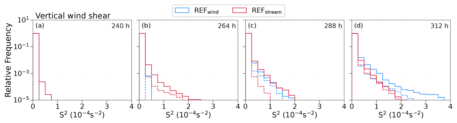
Figure 7 The temporal evolution of PDFs of vertical wind shear, S², in the lowermost stratosphere for dry reference experiments. The dashed histograms represent shear perturbations $S^{{\mathrm{2}}^{\prime }}$ from the spectral domain for the respective REF simulations.

In our analysis of shear and turbulence, we initially focus on the lowermost stratosphere. The lower boundary of LMS is defined here by the 3.5 PVU dynamical tropopause, whereas the 380 K isentropic level serves as an upper boundary, which corresponds to the height of the tropical lapse rate tropopause (e.g., Holton et al., 1995; Shepherd, 2007). This is the region in the extratropics where the mixing layer resides (e.g., Hoor et al., 2004). We start our analysis with probability density functions (PDFs) of N², S², and $S^{{\mathrm{2}}^{\prime }}$, where $S^{{\mathrm{2}}^{\prime }}$ represents small-scale shear defined as the deviation from the background vertical shear, in the LMS (Fig. 7). We focus on the time with significant GW activity, i.e., from 240 h onward, in the dry reference simulations (refer to Sect. 3.1). Here, two important implications become evident. First, the distribution of static stability is relatively constant with time and the perturbation method (Fig. A1). Second, the distribution of S² in Fig. 7a–d shows temporal variation in the positive tail of the distribution, whereas $S^{{\mathrm{2}}^{\prime }}$ majorly follows the trend of S². There is an increase in the occurrence of S² maxima with time, particularly during the strong GW activity. Although the changes in S² PDFs differ between the two perturbation methods, both exhibit a similar overall behavior. Notably, the increase in S² and particularly $S^{{\mathrm{2}}^{\prime }}$ is temporally aligned with the occurrence of GWs in the simulations. Under the assumption that $S^{{\mathrm{2}}^{\prime }}$ is strongly under the influence of GW activity, this, in turn, suggests a substantial contribution of GW to the generation of the largest shear values. This also reveals that the major part of total S² in the LMS resembles the small-scale shear.

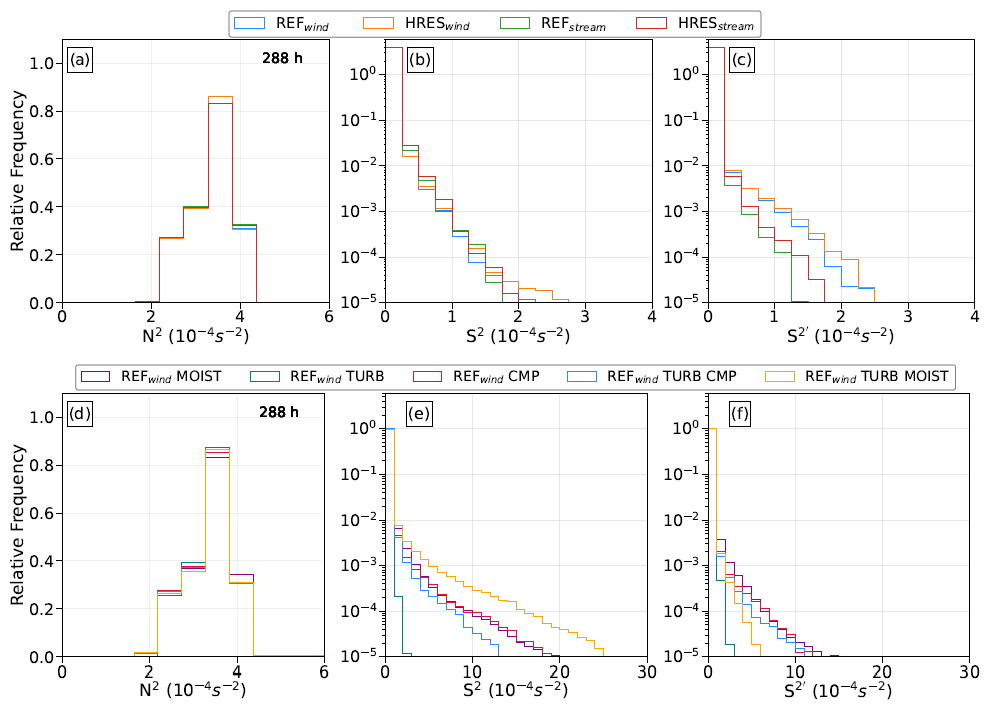
Figure 8 Temporal evolution of the relative occurrence frequency distribution of N² (a, d), S² (b, e), and $S^{{\mathrm{2}}^{\prime }}$ (c, f) in the lowermost stratosphere over the Northern Hemisphere. Upper panels (a–c) represent grid spacing sensitivity experiments. Lower panels (d–f) represent physics sensitivity experiments performed using the wind perturbation function. LMS is defined as the region between 3.5 PVU, a dynamical tropopause, and the 380 K isentropic surface.

An analysis of the N², S², and $S^{{\mathrm{2}}^{\prime }}$ PDFs for our sensitivity experiments with respect to grid spacing (Fig. 8a–c) and physical forcing (Fig. 8d–f) further suggests that GW may play a dominant role in the generation of the largest shear values. While the distributions of static stability in the LMS show comparable distributions among the sensitivity simulations (Fig. 8a and d), notable differences between the simulations arise for total shear (Fig. 8b and e) and for small-scale vertical shear (Fig. 8c and f). These differences can be summarized as follows: the finer grid spacing leads to more enhanced shear values, while moist dynamical processes drastically enhance the maximum shear values. However, the intense S² observed in TURB MOIST results in relatively fewer $S^{{\mathrm{2}}^{\prime }}$ occurrences in the spectral domain, likely due to enhanced turbulence indicated by the turbulent kinetic energy (TKE), which suppresses small-scale variability in shear. These findings align with our observations of GW appearance discussed in Sect. 3.2 and 3.3, further supporting the hypothesis that GWs play a key role in generating the largest shear values in the LMS in our BLC experiments.

To better understand the physical mechanism behind the contribution of GWs, we consider the vertical propagation behavior of GWs in a strongly stratified environment. The enhanced shear in the LMS is plausibly linked to the presence of upward-propagating GWs. As these waves cross the tropopause, the strong vertical gradient in the buoyancy frequency could lead to a shortening of the vertical wavelength of GWs. This, in turn, increases the vertical gradients of horizontal wind perturbations and thereby enhances local vertical wind shear. This interpretation is consistent with the theoretical framework described in Wei and Zhang (2015).

4.2 Dynamic instability and turbulence

On smaller scales and in instantaneous considerations, we observed significant general co-location of enhanced GW activity and enhanced S² and $S^{{\mathrm{2}}^{\prime }}$ occurrences in the LMS. Now, we move our discussion to the potential occurrence of turbulence in the LMS and additionally discuss the relation between N², S², $S^{{\mathrm{2}}^{\prime }}$, and Ri using a two-dimensional density function (following Fig. 14 in Kaluza et al., 2021). Turbulence is a rare event under general atmospheric conditions (Sharman et al., 2012; Dörnbrack et al., 2022), even in the LMS, and is even rarer than enhanced vertical shear. As such, only a few data points are expected to exhibit small-scale turbulence. This becomes evident when using two-dimensional probability density distributions with the axes being the squared Brunt–Väisälä frequency N² and the vertical shear of the horizontal wind (i.e., S² or $S^{{\mathrm{2}}^{\prime }}$). The color shows the relative frequency of N² and S² values in the LMS with respect to Ri (Fig. 9). We also added black dashed lines to mark values for the gradient Richardson number. For Ri ≤ 5, an indication of potential for the occurrence of dynamic instability is given. We adopt a threshold of Ri ≤ 5 to identify regions with enhanced potential for turbulence, considering previous studies (e.g., Lane et al., 2003; Olsen et al., 2013; Wang and Fu, 2021; Kunkel et al., 2019; Kaluza et al., 2021) and accounting for resolution-dependent effects (e.g., Shao et al., 2023). This threshold ensures consistent comparison across different grid spacings from 13 to 80 km, where small Ri values close to 1 are less likely, particularly in the lower stratosphere (Kaluza et al., 2022). The most unstable and/or potential turbulent regions are still captured using a more conservative threshold of Ri ≤ 1. Note that only data points in the LMS are considered for this analysis. Thus, we analyze only the turbulence and enhanced shear occurrence above the local 3.5 PVU dynamical tropopause and below 380 K. We also note that we focus on individual time steps and compare the PDFs for various simulations, which again helps to highlight the differences among the simulations.

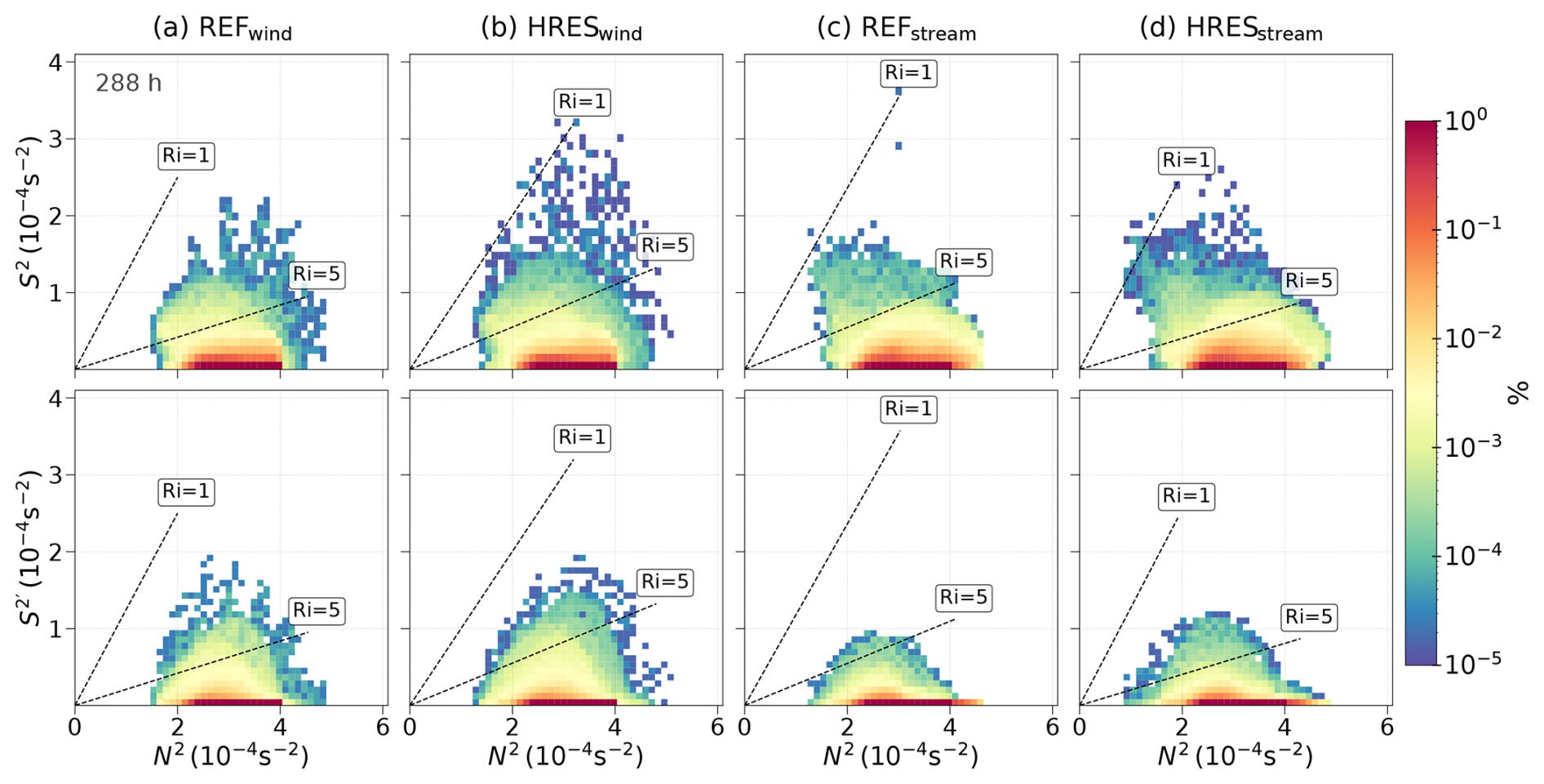
Figure 9 Relative occurrence frequency distribution of N²–S² (upper panel) and N²–$S^{{\mathrm{2}}^{\prime }}$ (lower panel) pair plot after 288 h for simulations with varying grid sensitivity over the Northern Hemisphere in the lowermost stratosphere. A logarithmic occurrence frequency color scale is applied. Dashed lines indicate the gradient Richardson numbers.

We start again with the dry adiabatic reference experiments and their high-resolution companions (REF and HRES; see Fig. 9). The results show that turbulence and enhanced shear are rare events, with few grid volumes falling below Ri≤1. For wind perturbations, HRES produces more regions of enhanced S² and tends to exhibit slightly more turbulence-prone areas compared to the REF simulation, highlighting the stronger influence of higher resolution in capturing these features. In contrast, stream perturbations show greater similarity between HRES and REF, with only a marginally enhanced total as well as small-scale shear and turbulence occurrences in HRES. Overall, S² and $S^{{\mathrm{2}}^{\prime }}$ show only minimal differences in the values but with the same magnitude, indicating that smaller scales contribute substantially to the total shear occurrence. HRES captures finer details and shows slightly more enhanced shear and turbulence than REF, as expected, with smaller scales contributing significantly to these enhanced values and low Ri occurrence. The dynamically stable LMS persists throughout most of the simulation, with a brief indication of potential turbulence during wave breaking. This indicates that the dry experiments exhibit evidence of potential dynamical instability in the LMS, with GWs as a potential contributor to turbulence generation.

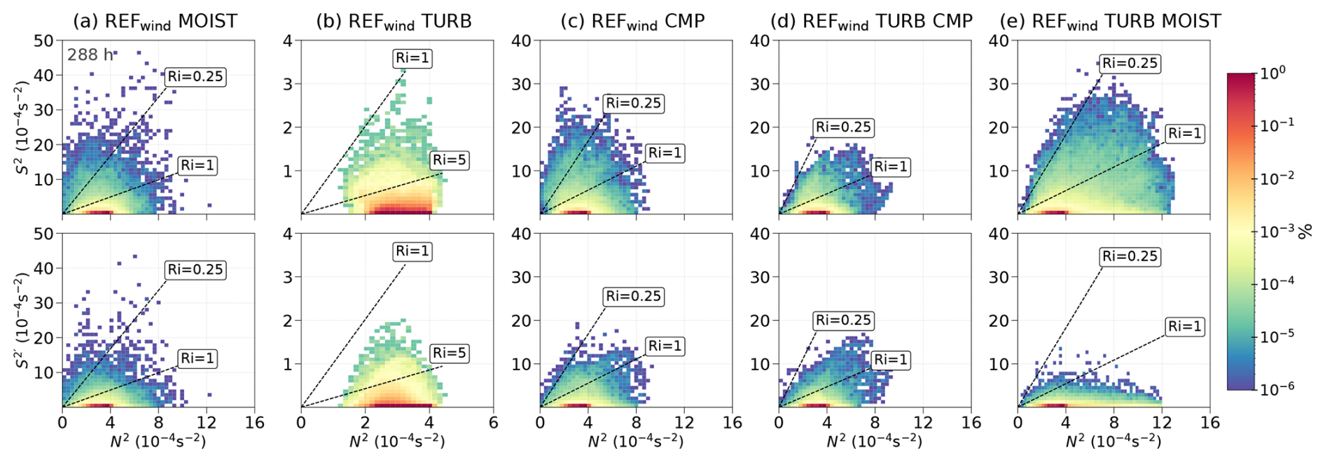
Figure 10 Same as in Fig. 9 but after 288 h for the REF_wind simulations with varying physical processes.

Figure 10 continues to demonstrate the temporal evolution of N²–S² pairs with Ri in sensitivity experiments with physical processes. The observed latent heating, i.e., REF_wind MOIST (Fig. 10a), is shown to increase the occurrence of enhanced shear in the LMS. The N²–S² (upper panel) and N²–$S^{{\mathrm{2}}^{\prime }}$ (lower panel) pairs show all cases with moisture that Richardson numbers below $\mathrm{1}/\mathrm{4}$ occur. The shear values reach up to 10 times higher than in the dry cases, as also evident in Figs. 7 and 8, which show consistently lower shear values in the dry simulations compared to the moist cases. Thus, moist processes in the troposphere seem to be eminently important for the occurrence of dynamic instability in the LMS, at least to the point that moist processes substantially increase the probability of an instability to form. In contrast, the inclusion of the turbulence scheme in the model setup reduces this probability again. The case of REF_wind TURB still shows more occurrence of low Richardson numbers than the corresponding dry case, but TKE can also be produced. The shear, in a way, also contributes to the enhanced values of TKE and might thus explain its enhancements and vice versa. REF_wind CMP and MOIST show that strong $S^{{\mathrm{2}}^{\prime }}$ values dynamically correlate with the larger N² in the vicinity of Ri≤5, indicating strong signatures of dynamic shear instability. Shear instability occurs when the vertical wind shear is large enough to overcome the tendency of stratified flow to remain stratified, after which KHI and vortexes form. These instabilities generally result from strong temperature gradient and wind shear induced by GWs (Fritts and Alexander, 2003). REF_wind TURB CMP mirrors the behavior of REF_wind CMP. Noticeable here in REF_wind TURB MOIST is the appearance of lower Ri attributed to latent heat release as discussed in Sect. 3.3. The turbulence counteracts the effects of dry dynamics, which enhance the lower stratospheric static stability (Koch et al., 2005).

Moreover, due to the tendency of turbulence to reduce the strong vertical gradients, a lower vertical shear is expected in this case. However, the TURB MOIST case shows much less potential turbulence from the small scales, even compared to its companion simulation CMP TURB. It is remarkable that, in this case, the N²–S² distribution differs substantially from the N²–$S^{{\mathrm{2}}^{\prime }}$ distribution. Thus, much of the potential turbulence in TURB MOIST is evident on larger scales. To further demonstrate this, the vertical distribution of TKE is found to be enhanced by a factor of 50 in TURB MOIST compared to TURB CMP and TURB (see Fig. S6). There are two sources for the generation of TKE: first, the vertical shear, and second, the vertical gradient of total moisture, which can consequently lead to buoyant heat flux (Doms et al., 2011). Although the vertical shear (both small- and large-scale) was observed to be similar in all turbulence-included cases, the subsequent buoyant heat flux in TURB MOIST shows positive and negative values for the region of larger TKE values (Fig. S6) around the tropopause, most probably related to Rossby waves, as it is linked to large-scale flow features rather than small-scale GW activity. Due to this, the N²–$S^{{\mathrm{2}}^{\prime }}$ spectrum shows a drastic decrease in grid volumes associated with low Ri. Ultimately, there is the existence of a large overlap between enhanced small-scale shear and a low Richardson number, as well as GW activity. Altogether, the occurrence of low Ri is primarily driven by shear induced by large-amplitude GWs, as evidenced by localized regions of strong small-scale wind shear despite moderate background shear. This is further supported by the similarity in the distributions of S² and $S^{{\mathrm{2}}^{\prime }}$ in the LMS, particularly in the upper tail of the PDFs (as shown in Fig. 8b, e and c–f).

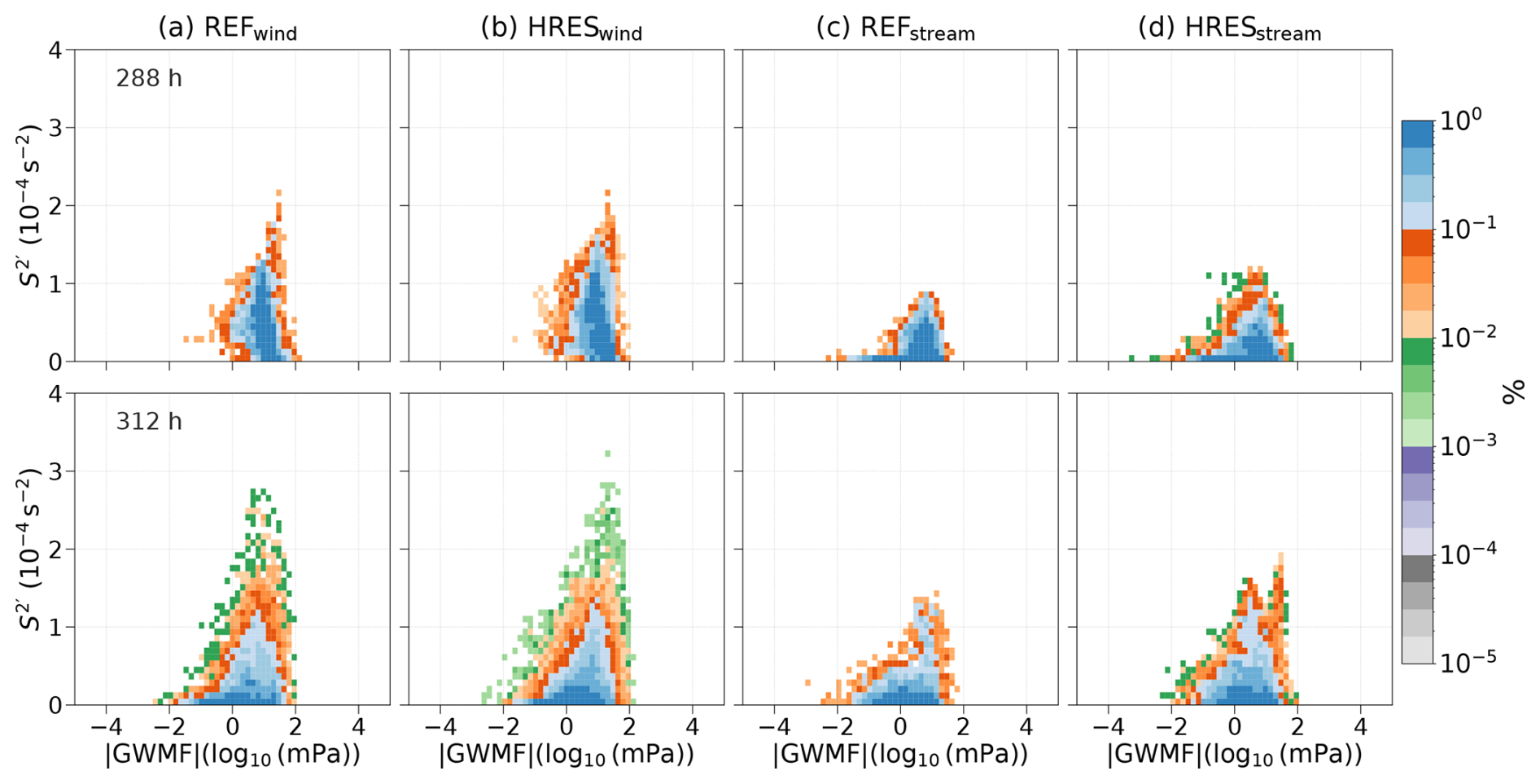
Figure 11 Relative occurrence frequency or probability density distribution of the absolute momentum flux due to the GWs $\left|\mathrm{GWMF}\right|$–vertical shear perturbations $S^{{\mathrm{2}}^{\prime }}$ pair in the LMS for Ri≤5 after 288 h (upper panel) and 312 h (lower panel) for simulations with grid spacing sensitivity. Normalized counts of the PDF distribution are given. A logarithmic occurrence frequency color scale is applied.

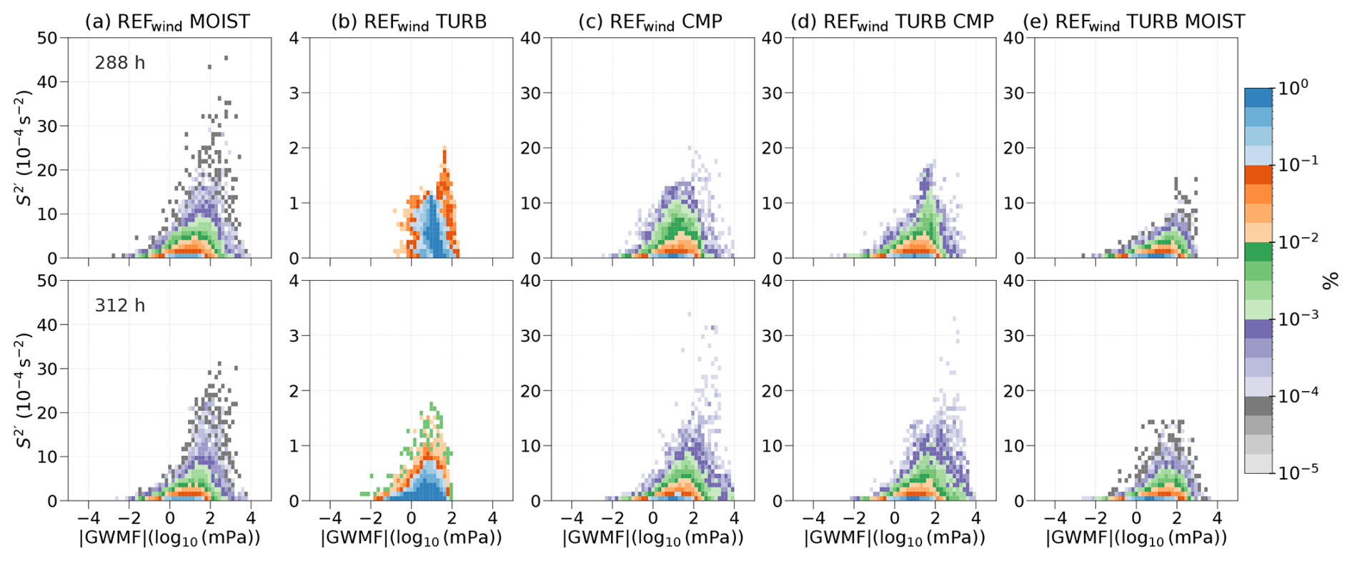
Figure 12 Same as in Fig. 11 but for simulations with physical processes sensitivity. Normalized counts of the PDF distribution are given. A logarithmic occurrence frequency color scale is applied.

We will further explore this relation through the inclusion of the small-scale momentum flux (Figs. 11 and 12). If the small scales play a major role in the shear and turbulence generation, then we expect a positive correlation between $S^{{\mathrm{2}}^{\prime }}$ and absolute GWMF in the case of turbulence occurrence. When we filter the data of our simulations for potential turbulence, i.e., Ri≤5 in the LMS, we find a positive correlation. We interpret this as an indication that the small scales and, here in particular, the GWs contribute substantially to the occurrence of strong large-scale as well as small-scale shear and potential turbulence. This relation is evident in the dry simulations, also across the various sensitivity experiments (see Fig. 11 for the RES and HRES experiments), as well as for the sensitivity simulations with physics (see Fig. 12). Note here that the results are not strongly dependent on the wavenumber used to separate the background from the small scales.

Overall, our results strongly highlight the important role of GWs in determining potential turbulence in the LMS. Consequently, they might also play a vital role in turbulent mixing of trace species in this region and thus in the formation of the extratropical transition layer (Hoor et al., 2004; Pan et al., 2006). Because the potential turbulence occurrence is strongly linked to enhanced shear, we will explore in the next section in more detail the role of the small-scale dynamics in the formation of the tropopause wind shear layer.

5 Occurrence of TSL and associated GWs

Up to this point, the discussion has centered on enhanced shear generation, as well as the potential for turbulence occurrence and consequent mixing. In this section, we shift our focus to the occurrence of the tropopause shear layer (TSL) in the extratropics and its potential association with GWs in the LMS. The TSL has been defined by exceeding a defined threshold value of vertical wind shear. In Kaluza et al. (2021), the authors calculated the occurrence frequency of such shear exceeding a defined threshold in the tropopause-following coordinate over a 10-year dataset for the Northern Hemisphere. Here, we adopt this approach for our data but do the analysis at an instantaneous time step. Our goal is to show that the occurrence frequencies of enhanced vertical wind shear are temporally aligned with the presence of GW in the LMS. Note that in this case, we use the total shear S² derived from the full wind components. In contrast to Kaluza et al. (2021), we start from a state with no TSL, which allows us to analyze the temporal evolution of the shear in the LMS. We follow the steps outlined in Kaluza et al. (2021) but with some adaptions for our simulations.

The identification of the tropopause shear layer requires the definition of a threshold value for S². We follow the method used by Kaluza et al. (2021) with adaptation to our BLCs. In particular, the threshold value is selected based on the criterion that S² ≥ $S_{\mathrm{t}}^{\mathrm{2}}$ is typically unsustainable under the average tropospheric static stability $\left(\stackrel{\mathrm{‾}}{N_{\mathrm{trop}}^{\mathrm{2}}}\right)$, which results in low Ri and conditions favorable for potential turbulence. Following this, and considering the average tropospheric static stability $\stackrel{\mathrm{‾}}{N_{\mathrm{trop}}^{\mathrm{2}}}\approx \mathrm{2}\times {\mathrm{10}}^{-\mathrm{4}}$ s⁻² for simulations incorporating physical processes, we use a threshold value $S_{\mathrm{t}}^{\mathrm{2}}$ = $\mathrm{2}\times {\mathrm{10}}^{-\mathrm{4}}$ s⁻², consistent with Kaluza et al. (2021), where latent heating enhances GW activity and shear occurrences. In contrast, dry simulations exhibit a much lower mean tropospheric static stability value $\mathrm{0.1}\times {\mathrm{10}}^{-\mathrm{4}}$ s⁻² due to the prescribed temperature profile of the idealized setup. To adequately capture the full range of dynamically relevant shear in these weakly stable conditions, we adopt a lower threshold of $\mathrm{0.3}\times {\mathrm{10}}^{-\mathrm{4}}$ s⁻². This value is supported by sensitivity tests, which showed that increasing the threshold (e.g., $\mathrm{1}\times {\mathrm{10}}^{-\mathrm{4}}$ s⁻²) significantly reduced the frequency of identified shear occurrences but did not change the overall distribution patterns. Thus, for dry experiments, the chosen threshold accounts for inherently low shear occurrences and ensures that the full spectrum of shear is captured. Therefore, our selected thresholds reflect the underlying differences in static stability and shear environments between dry and moist simulations while maintaining consistency with an established physically based criterion. Note that these values are much lower than the threshold defined in Kaluza et al. (2021), which is mainly rooted in the idealized setup compared to a fully comprehensive reanalysis system.

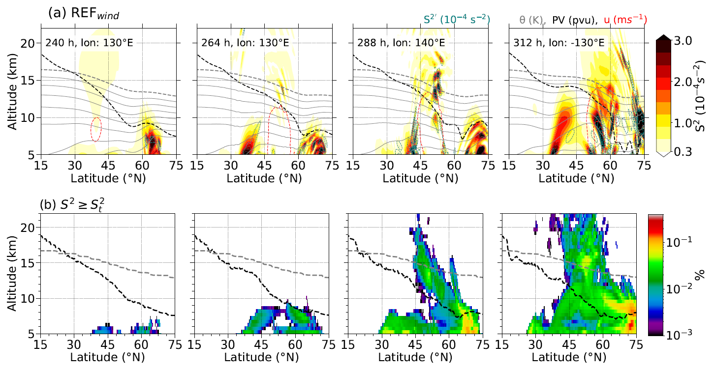
Figure 13 The temporal evolution of (a) the vertical cross section of shear through the identified regions of GWs from time 240 h onward for the REF_wind simulation with $S^{{\mathrm{2}}^{\prime }}$ (dashed green), potential temperature (gray), zonal wind (30 m s⁻¹, red), and dynamical tropopause (black) and (b) the respective Northern Hemispheric occurrence frequency distribution of grid volumes that exhibit S² ≥ $S_{\mathrm{t}}^{\mathrm{2}}$. A logarithmic frequency contour, vertically binned in dz = 500 m, is applied. The zonal mean value of 3.5 PVU in the potential vorticity field is indicated by the dashed black line, and the zonal mean value of 380 K in the potential temperature field is indicated by the gray dashed line.

Figure 13a demonstrates the temporal evolution of the vertical cross section of shear S², zonal wind u, PV, and potential temperature. The corresponding wave signals at an altitude of 11 km are indicated by a dashed line in Fig. 6a). Notably, the region of S² is strongly affected by a small-scale wave pattern related to an upward-propagating GW, evident in the potential temperature and PV isolines. Meanwhile, the spatiotemporal overlap of GW signatures and $S^{{\mathrm{2}}^{\prime }}$, particularly after 288 h, indicates that GW is an important, if not the major, source of the enhanced values of shear occurrence in the LMS. Figure 13b shows the temporal evolution of relative occurrence frequency counted in the zonal direction for the vertical wind shear S² ≥ $S_{\mathrm{t}}^{\mathrm{2}}$ on a logarithmic color scale for the Northern Hemisphere, with the geometric altitude as the vertical coordinate. Figure 13b reveals regions of distinct occurrence frequency located in UTLS: one in the mid-latitudes between 40 and 55° N and another between 60 and 75° N above the dynamical tropopause in the extratropics. The progression of enhanced shear over time, with significant enhancement in the LMS, appears to follow the occurrence of the GW in the BLC and is tightly linked to the breaking of the synoptic scale wave. We note here that the REF_stream simulation exhibits a similar pattern. As discussed in Sect. 3.4 and in the paragraph above, the growing GW trains amplify S² maxima and induce shear in the extratropics, with upward-propagating GWs inducing pronounced shear in the vicinity of the tropopause and the LMS. This overlap between the pronounced shear occurrence and GW activity through the lower stratosphere strongly proposes that GWs are the source of enhanced shear generation in the LMS.

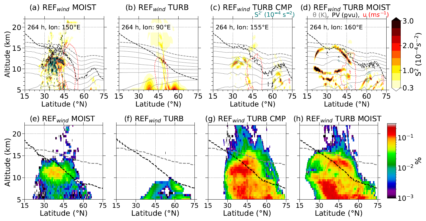
Figure 14 Vertical cross section of shear (a–d) through the identified regions of GWs in the 264 h REF_wind simulations with physical processes sensitivity and the respective Northern Hemispheric occurrence frequency distribution of the grid volumes that exhibit S² ≥ $S_{\mathrm{t}}^{\mathrm{2}}$ (e–h). A logarithmic frequency contour, vertically binned in dz = 500 m, is applied. The zonal mean dynamical tropopause altitude is indicated by the dashed black line, and the tropical tropopause (380 K isentrope) is indicated by the gray dashed line.

Furthermore, an analysis of TSL occurrence across sensitivity experiments, including grid spacing (not shown) and physical forcing (as shown in Fig. 14), also suggests that GWs play a dominant role in generating enhanced vertical shear. For the simulations with moisture and turbulence parameterization, we see a similar temporal evolution of the vertical shear in the UTLS. Major differences are related to the TURB CMP and TURB MOIST showing firm S² ≥ $S_{\mathrm{t}}^{\mathrm{2}}$ occurrences due to contributions from sub-synoptic features and enhanced turbulent processes. Here, the vertical shear distribution broadens with altitude, shifting toward higher values, with the peak shear predominantly concentrated in the extratropical upper troposphere (see Fig. 14). This peak shear occurrence just below the tropopause, as noted by Kaluza et al. (2022), aligns with the sharp unimodal turbulence distribution. The observed colocation of shear generated by GWs and peak shear occurrence in the UT reveals the substantial contribution from small-scale features, particularly GWs, along with moist tropospheric dynamics.

Overall, these findings support the hypothesis that GWs contribute to enhanced shear occurrence, that is, the tropopause wind shear layer in the extratropical LMS. Broadly speaking, our results suggest that GWs play a pivotal role in shaping TSL dynamics and consequently contribute to the formation and maintenance of the ExTL.

6 Summary and conclusion

In this study, we investigate the role of GWs in generating vertical wind shear and potential turbulence and their contribution to the formation of regions of enhanced vertical shear in the extratropical lowermost stratosphere. Using idealized baroclinic life cycle experiments with ICON, we examine the impact of model grid spacing and non-conservative processes including moisture, cloud microphysics, and turbulence on the GW emergence and the generation of shear. Our findings emphasize that GWs, driven by baroclinic wave dynamics, are pivotal in enhancing vertical wind shear and promoting turbulence in this region. This highlights several key implications of GWs regarding vertical shear generation:

1. The appearance and associated shear of GWs are highly dependent on the model grid spacing. A distinct change in the emergence of GWs occurs when a horizontal model grid spacing finer than 20 km is applied. Moreover, and also less important in our case, we see more GW signs with shorter wavelengths for the vertical grid spacing currently used in numerical weather prediction (NWP) models, i.e., dz ∼ 300 m, compared to simulations with dz ∼ 1 km. This highlights the necessity to properly simulate GWs and to capture small-scale processes considering suitable higher spatial resolution. In addition, using the DCMIP initial states in both forms of wind and stream perturbations gives similar evolution of the GW life cycles and leads to the same conclusion in terms of the role of GWs in shear and potential turbulence generation in the UTLS.

2. Physical processes, such as moisture and latent heat release in the troposphere, significantly influence the extent and occurrence of GWs and thus shear and turbulence occurrence in the LMS. MOIST simulations revealed that latent heat release in the troposphere enhances GWs near the tropopause, leading to substantial shear enhancement in the lower stratosphere. These results are quite robust for different model settings in terms of spatial and temporal resolution and physics parameterizations. This gives further confidence that GW breaking is of relevance for the overall occurrence of enhanced shear in the lowermost stratosphere.

3. Further indication of the role of GWs for shear and turbulence generation in the LMS is found through a spatiotemporal correlation between small-scale momentum flux, enhanced shear, and low Richardson numbers. This correlation is independent of our model configuration and is found in dry, moist, and turbulent experiments of baroclinic waves.

4. The occurrence frequency of strong vertical shear near the tropopause peaks in extratropical LMS and correlates with GW activity, suggesting that GWs amplify shear maxima and lead to shear enhancement near the tropopause. TSL analysis highlights that upward-propagating GWs are a major contributor to enhanced vertical shear in the LMS, particularly associated with the breaking of synoptic-scale baroclinic waves.

Regarding point 2, the sudden shear enhancement in moist experiments is due to the latent heating release and its effect on the overall evolution of the baroclinic wave. The faster evolution of the baroclinic wave, along with stronger upward motions, substantially affects the presence of GWs in the LMS in terms of number, magnitude, and growth rate. Furthermore, our results support the hypothesis that grid spacing sensitivity is mainly influenced by horizontally propagating GWs with large horizontal wavelengths, which dominate the horizontal derivatives of momentum fluxes, while upward-propagating large-amplitude GWs contribute predominantly to the vertical derivatives of the wind components. This, in turn, leads to much higher shear values and lower Richardson numbers, i.e., more regions prone to becoming dynamically unstable. Ultimately, this highlights the role of tropospheric dynamics for the potential mixing of air masses due to small-scale dynamics in the LMS.

Further investigation into the relationship between GWs and TSL is warranted, as both appear consistently in climatological data based on zonal and temporal tropopause averages (Birner et al., 2002; Zhang et al., 2019). The enhanced shear associated with GWs is key for the emergence of the shear layer above the extratropical tropopause and, thus, a crucial feature in the formation and maintenance of the extratropical transition layer, a region identifiable through chemical tracer observations (e.g., Hoor et al., 2004; Pan et al., 2006; Birner, 2006). It is found that the GWs originating from baroclinic waves are pivotal in shaping the structure and dynamics of the extratropical LMS. The observed GW momentum flux and enhanced zonal shear correlation support the dominant role of GWs in TSL development, highlighting their potential influence on STE, turbulent mixing, and ultimately the distribution of chemical species in the tropopause region.

Despite the valuable insights gained in this study, there are some limitations that should be acknowledged. First, the use of an idealized setup with short simulation times and specific initial states does not account for seasonal and inter-annual variations. Additionally, GWs from other sources, such as orography and convection, are not considered, and the representation of the GW spectrum may be insufficient to fully capture the complexity of small-scale GW dynamics. These limitations suggest that further investigation is needed to comprehensively understand the role of GWs in shear enhancement and turbulent mixing in the LMS. To address these gaps, future work could build upon this study by simulating real-case scenarios using more comprehensive model setups, including processes like convection and improved GW parameterizations. Conducting longer simulations would allow for a better understanding of the processes driving the TSL and capturing seasonal and inter-annual variations. Moreover, generating a climatological dataset of small-scale GWs in the UTLS, validated by long-term observational data, would provide valuable guidance on the sources contributing to the TSL and their broader atmospheric implications. On the other hand, validation of these results using orographic and non-orographic GW parameterizations might help to thoroughly explain the role of GWs in STE and mixing in the LMS.

Overall, our findings highlight the crucial role of GWs in the enhancement of vertical shear and in facilitating potential turbulent mixing in the extratropical LMS, ultimately contributing to the formation of the extratropical transition layer. These results underscore the importance of accounting for GWs in the prediction of clear air turbulence, as their influence on unforeseen turbulence events cannot be neglected. This opens the door for further exploration of how subgrid-scale GWs influence vertical shear and transport processes in the UTLS, particularly their role in the tropopause shear layer and stratosphere–troposphere exchange.

Appendix A: Supporting information for the shear and turbulence diagnostics in the LMS

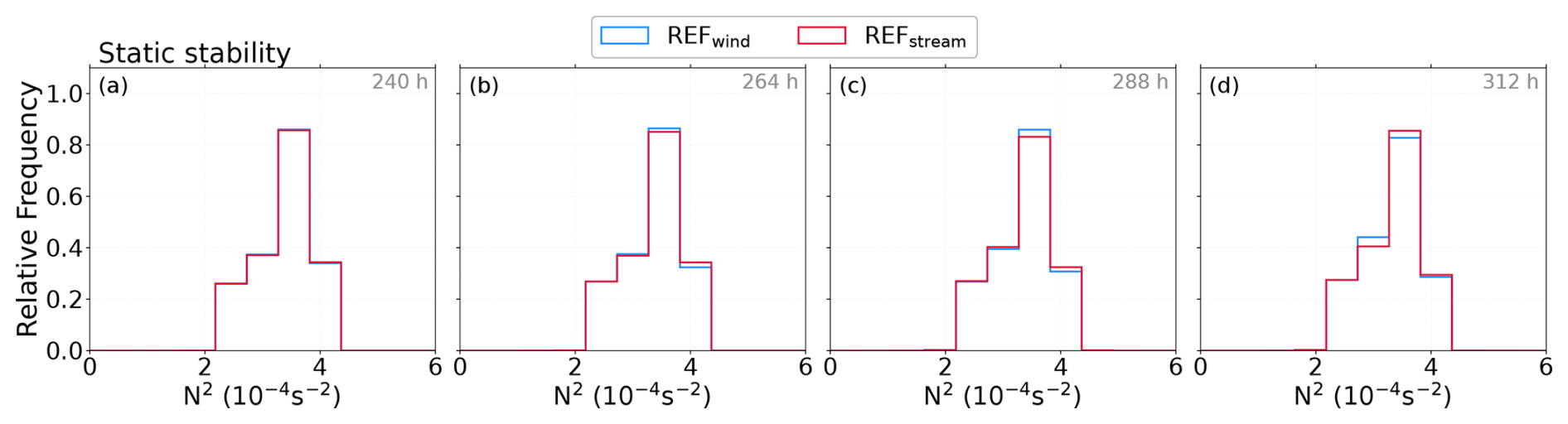
Figure A1 The temporal evolution of PDFs of static stability, N², in the lowermost stratosphere for dry reference experiments.

Appendix B: Supporting information for latent heat release in MOIST experiments

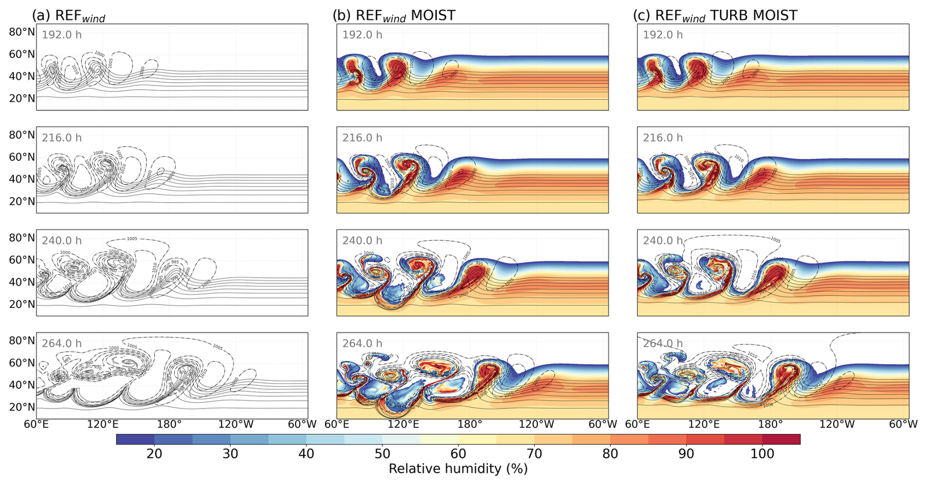
Figure B1 Time evolution from 192 to 264 h of surface pressure (dashed contours), surface potential temperature (solid contours, every 5 K), and (for the moist simulation only) RH at 850 hPa (colored, %). (a) REF_wind, (b) REF_wind MOIST, and (c) REF_wind TURB MOIST simulations.

As for the latent heat release, we use relative humidity (RH) at 850 hPa as a quasi-proxy for latent heat release. Figure B1 shows the evolution of surface pressure and surface potential temperature for the dry REF, MOIST, and TURB MOIST simulations from 192 to 264 h of the model run. For MOIST simulations, the relative humidity at 850 hPa is shown. In the MOIST cases, the onset of frontogenesis around 192 h is accompanied by progressive humidification in the warm sector of the developing cyclone. RH values rise to above 80 %, with localized saturation (RH ≥ 90 %) along and ahead of the warm front, indicative of sustainedlifting and associated condensation processes. After 216 h, as the cyclone matures and enters the frontal fracture stage, the structural differences between the dry and moist simulations become more evident. The bent-back segment of the warm front in the MOIST simulation exhibits elevated RH alongside intensified horizontal temperature gradients. This spatial alignment reflects dynamically consistent latent heating, contributing to stronger pressure gradients and the development of a low-level wind maximum. At this point, the central sea level pressure in the MOIST runs falls below 965 hPa, compared to ∼ 970 hPa in the REF simulation. After 240 h, RH values in the primary cyclone remain elevated across both warm and cold frontal regions, suggesting ongoing moist processes. Importantly, the downstream cyclone in MOIST also shows RH exceeding 90 % in its core, despite forming later in the BLC, implying that in situ latent heating plays a key role in its intensification. While the primary baroclinic wave evolution remains largely controlled by dry dynamics in the early stages, the differences in cyclone intensity, frontal structure, and secondary cyclone development in the moist runs point to the substantial dynamical role of latent heating.